Extremes of joint inversions and descents on finite Coxeter groups

Abstract.

The numbers of inversions and descents of random permutations are known to be asymptotically normal. On general finite Coxeter groups, the central limit theorem (CLT) is still valid under mild conditions. The extreme values of these two statistics are attracted by the Gumbel distribution. The joint distribution of inversions and descents is a likewise interesting object, but only the CLT on symmetric groups has been established thus far. In this paper, we comprehensively extend the knowledge of the joint distribution of inversions and descents. We prove both the CLT and the extreme value attraction for the joint distribution of inversions and descents by using Hájek projections and a suitable Gaussian approximation. On the signed permutation groups, we additionally show that these results are still valid when the choice of the random signs is biased. Furthermore, we investigate the applicability of these techniques to products of classical Weyl groups.

1. Introduction

The numbers of inversions and descents are two of the most important characteristics of permutations or, more generally, of Coxeter group elements. On the symmetric group $S_{n}$ of permutations $\pi\negmedspace:\{1,\ldots,n\}\rightarrow\{1,\ldots,n\},$ an inversion is any tuple $(i,j)$ with $i<j,$ but $\pi(i)>\pi(j)$. A descent is any inversion of two adjacent numbers, that is, any $i$ with $\pi(i)>\pi(i+1)$. Symmetric groups belong to the class of finite Coxeter groups, on which the concept of inversions and descents can be readily generalized, see [3, Section 1.4]. We can treat the underlying Coxeter group as a probability space and draw its elements at random. The study of stochastic properties of quantities such as the number of inversions and descents belongs to the field of statistical algebra and is the aim of this paper. We use the notations $X_{\mathrm{inv}}$ and $X_{\mathrm{des}}$ to indicate the nature of these numbers as random variables. In all following scenarios, we suppose that elements of a symmetric group or finite Coxeter group are drawn uniformly at random, unless stated otherwise. For some basics on finite Coxeter groups, we refer to [3].

This paper will focus on the classes $S_{n}$ (symmetric groups), $B_{n}$ (signed permutation groups) and $D_{n}$ (even-signed permutation groups), for which we use the umbrella term classical Weyl groups throughout.

The asymptotic distribution of $X_{\mathrm{inv}}$ and $X_{\mathrm{des}}$ has been investigated by several authors (see, e.g., [2, 6, 16, 17, 18, 23]), who showed that inversions and descents each satisfy a central limit theorem (CLT) and thus are asymptotically normal. We say that a family of real-valued random variables $X_{1},X_{2},\ldots$ (or their respective distributions) satisfies the CLT if

$$\frac{X_{n}-\mathbb{E}(X_{n})}{\mathrm{Var}(X_{n})^{1/2}}\overset{\mathcal{D}}{\longrightarrow}\mathrm{N}(0,1)\,,\qquad n\to\infty\,,$$

where $\overset{\mathcal{D}}{\longrightarrow}$ denotes convergence in distribution. If the $X_{n}$ are sums of independent random variables, one can verify the classical Lindeberg or Lyapunov conditions to establish a CLT.

For the number of inversions or descents on finite Coxeter groups, there are several techniques and approaches toward the CLT. Chatterjee & Diaconis provide an overview of proofs of the CLT for $X_{\mathrm{des}}$ on the family of symmetric groups in [6, Section 3]. One approach is based on a representation of $X_{\mathrm{des}}$ via $m$-dependent variables, which will be essential for our own methods in Section 2. Alternative proofs of the asymptotic normality of $X_{\mathrm{des}}$ are based on the zeros of its generating function [17, 23] or on certain regularity properties of the generating function, see [2, Ex. 3.5 and 5.3]. Stein’s method of exchangeable pairs has been applied in [10, 16], where the latter reference and [2, Ex. 5.5] also cover inversions. We note that Stein’s method has been used in various settings, see, e.g., [11] for permutations on multisets, [22] for generalized inversions, and [1] for non-uniformly random permutations.

Kahle & Stump [18] developed a full characterization of CLTs for inversions and descents on sequences of finite Coxeter groups, by giving necessary and sufficient conditions on the asymptotics of $\mathrm{Var}(X_{\mathrm{inv}})$ and $\mathrm{Var}(X_{\mathrm{des}})$. The work of Dörr & Kahle [13] was the first to provide extreme value theory for these classical permutation statistics. They showed that the numbers of inversions and descents are in the maximum-domain of attraction of the standard Gumbel distribution, assuming a triangular array where the number of samples per row obeys an exponential upper bound.

While the asymptotic normality of inversions and descents as univariate statistics is well studied, the knowledge of their joint distribution is comparatively sparse. Fang & Röllin [15] gave a CLT for arbitrarily large collections of permutation statistics based on antisymmetric matrices, including $(X_{\mathrm{inv}},X_{\mathrm{des}})$ as a special case. Their work can also be seen as a multivariate extension of [16]. The aforementioned papers based on Stein’s method typically achieve an $O(n^{-1/2})$ rate of convergence. Our novel approach will not achieve this rate, but it will generalize the multivariate CLT to other classical Weyl groups and even further, it will cover the asymptotic extreme value behavior of $(X_{\mathrm{inv}},X_{\mathrm{des}})$.

This paper is structured as follows. Section 2 introduces the Hájek projection of inversions and descents on symmetric groups and justifies its use to approximate $X_{\mathrm{inv}}$. Section 3 introduces the Gaussian approximation result on $m$-dependent random vectors by Chang et al. [5], which we use to prove the asymptotic normality of $(X_{\mathrm{inv}},X_{\mathrm{des}})$. Section 4 presents the corresponding extreme value limit theorem (EVLT) as the main result of this paper. In Section 5, these results are extended to the larger groups $B_{n}$ and $D_{n}$, which are equipped with a new family of probability measures, namely the so-called $p$-biased signed permutations. Section 6 studies the CLT and EVLT for direct products of classical Weyl groups, and Section 7 concludes the paper with some open questions. The remaining technical proofs are gathered in the appendix in Section 8.

Throughout this paper, we denote the standard uniform distribution on the interval $[0,1]$ by $U(0,1)$, and the discrete uniform distribution on the set $\{0,1,\ldots,n\}$ by $U(\{0,1,\ldots,n\})$. We sometimes also use these notations for accordingly distributed random variables when the meaning is clear from the context. The symbol $\stackrel{{\scriptstyle\mathcal{D}}}{{=}}$ means equality in distribution and $\sum_{i<j}$ will be used as an abbreviation of the double-indexed sum $\sum_{1\leq i<j\leq n}$. For any random variable $X$, we denote its standard deviation by $\sigma(X)=\sqrt{\mathrm{Var}(X)}$. Moreover, we use typical Landau notation for positive sequences $a_{n},b_{n}$ as follows:

• $a_{n}=O(b_{n})$ means that $a_{n}$ grows at most as fast as $b_{n}$, i.e., $\limsup_{n\rightarrow\infty}a_{n}/b_{n}<\infty$.

• $a_{n}=o(b_{n})$ means that $a_{n}$ grows slower than $b_{n}$, i.e., $\lim_{n\rightarrow\infty}a_{n}/b_{n}=0$. This is also written as $a_{n}\ll b_{n}$ or $b_{n}\gg a_{n}$.

• $a_{n}=\Theta(b_{n})$ means that $a_{n}$ and $b_{n}$ have the same order of magnitude, i.e., both $a_{n}=O(b_{n})$ and $b_{n}=O(a_{n})$ hold.

• $a_{n}=b_{n}+o_{\mathbb{P}}(1)$ means that $a_{n},b_{n}$ are sequences of random variables with $a_{n}-b_{n}\overset{\mathbb{P}}{\longrightarrow}0$.

2. Hájek projections on symmetric groups

A permutation drawn uniformly at random from the symmetric group $S_{n}$ of permutations on $n$ letters is induced by the ranks of independent random variables $Z_{1},\ldots,Z_{n}\sim U(0,1)$. Thus, the numbers of inversions and descents of this permutation can be represented by

(1) $$X_{\mathrm{inv}} =\sum_{1\leq i<j\leq n}\textbf{1}\{Z_{i}>Z_{j}\},$$

(2) $$X_{\mathrm{des}} =\sum_{i=1}^{n-1}\textbf{1}\{Z_{i}>Z_{i+1}\}.$$

The primary challenge in dealing with the joint permutation statistic $(X_{\mathrm{inv}},X_{\mathrm{des}})$ is the dependence structure between $X_{\mathrm{inv}}$ and $X_{\mathrm{des}}$. The random variables $\textbf{1}\{Z_{i}>Z_{j}\},1\leq i<j\leq n$ in (1) are also dependent. It is worth noting that $X_{\mathrm{inv}}$ has the following representation as a sum of $n-1$ independent terms:

(3) $$X_{\mathrm{inv}}\stackrel{{\scriptstyle\mathcal{D}}}{{=}}\sum_{i=1}^{n-1}U(\{0,1,\ldots,i\})\,.$$

This follows, e.g., from [13, Corollary 2.5a)] within the framework of all finite Coxeter groups. The representation of $X_{\mathrm{des}}$ in (2) has $m$-dependent variables (precisely, $m=1$). There is also a decomposition of $X_{\mathrm{des}}$ into independent summands, based on the splitting of its generating function (known as the Eulerian polynomial) into linear factors of its real-valued roots [13, Corollary 2.5b)].

From the representations in [13, Corollary 2.5a)] and [13, Corollary 2.5b)] it is easy to derive the generating functions of $X_{\mathrm{inv}}$ and $X_{\mathrm{des}}$. That $X_{\mathrm{inv}}$ and $X_{\mathrm{des}}$ are not independent follows from the fact that the joint generating function of $(X_{\mathrm{des}},X_{\mathrm{inv}})$ does not factor into those of $X_{\mathrm{inv}}$ and $X_{\mathrm{des}}$. It is an interesting question whether this polynomial factors at all. Some tests were made on $S_{3}$ or $S_{4},$ but there was no regularity detected so far.

To handle the dependence between $X_{\mathrm{inv}}$ and $X_{\mathrm{des}}$, we approximate $X_{\mathrm{inv}}$ through its Hájek projection $\hat{X}_{\mathrm{inv}}$ and write $(\hat{X}_{\mathrm{inv}},X_{\mathrm{des}})$ as a sum of $m$-dependent two-dimensional random vectors. Then, we apply a Gaussian approximation theorem by Chang et al. [5] for triangular arrays of $m$-dependent random vectors. This will give a new proof of the CLT, and more importantly, it will be essential to derive the extreme value limit theorem (EVLT) for $(X_{\mathrm{inv}},X_{\mathrm{des}})$ on classical Weyl groups.

Definition 2.1.

For independent random variables $Z_{1},\ldots,Z_{n}$ and any random variable $X_{n}$, the Hájek projection of $X_{n}$ with respect to $Z_{1},\ldots,Z_{n}$ is given by

$$\hat{X}_{n}:=\sum_{k=1}^{n}\mathbb{E}(X_{n}\mid Z_{k})-(n-1)\mathbb{E}(X_{n}).$$

Note that $\mathbb{E}(\hat{X}_{n})=\mathbb{E}(X_{n})$. Since each $\mathbb{E}(X_{n}\mid Z_{k})$ is a measurable function only in $Z_{k}$, the Hájek projection is a sum of independent random variables, regardless of the original dependence structure between $X_{n}$ and $Z_{k}$. In Sections 2–4, we always assume that $Z_{1},\ldots,Z_{n}\sim U(0,1)$ for our purposes. To decide whether the Hájek projection is a sufficiently accurate approximation, the following criterion is useful.

Theorem 2.2 (cf. [24], Theorem 11.2).

Consider a sequence $(X_{n})_{n\geq 1}$ of random variables and their associated Hájek projections $(\hat{X}_{n})_{n\geq 1}$. If $\mathrm{Var}(\hat{X}_{n})\sim\mathrm{Var}(X_{n})$ as $n\rightarrow\infty,$ then

$$\frac{X_{n}-\mathbb{E}(X_{n})}{\mathrm{Var}(X_{n})^{1/2}}=\frac{\hat{X}_{n}-\mathbb{E}(\hat{X}_{n})}{\mathrm{Var}(\hat{X}_{n})^{1/2}}+o_{\mathbb{P}}(1).$$

In particular, if $\mathrm{Var}(\hat{X}_{n})\sim\mathrm{Var}(X_{n})$ and $(\hat{X}_{n})_{n\geq 1}$ satisfies a CLT, then Theorem 2.2 guarantees that $(X_{n})_{n\geq 1}$ also satisfies a CLT.

In what follows, for a random variable or vector $X$ with finite variance, we write $Y$ for its standardization, that is, $Y=\bigl{(}X-\mathbb{E}(X)\bigr{)}/\sqrt{\mathrm{Var}(X)}$. In particular, $Y_{\mathrm{inv}}$ is the standardization of $X_{\mathrm{inv}}$ and $\hat{Y}_{\mathrm{inv}}$ is that of $\hat{X}_{\mathrm{inv}}$. We use the symbols $X_{\mathrm{inv}},Y_{\mathrm{inv}},\hat{X}_{\mathrm{inv}},\hat{Y}_{\mathrm{inv}},X_{\mathrm{des}},Y_{\mathrm{des}}$ with suppression of $n$, the underlying symmetric group or its rank, unless needed for clarification.

The next result provides the Hájek projection of $X_{\mathrm{inv}}$ defined in (1) and verifies the variance equivalence condition stated in Theorem 2.2 for $X_{\mathrm{inv}}$.

Lemma 2.3.

The Hájek projection $\hat{X}_{\mathrm{inv}}$ of $X_{\mathrm{inv}}$ is given by

$$\hat{X}_{\mathrm{inv}}=\frac{n(n-1)}{4}+\sum_{k=1}^{n}(n-2k+1)Z_{k}$$

and it holds that $\mathrm{Var}(X_{\mathrm{inv}})\sim\mathrm{Var}(\hat{X}_{\mathrm{inv}})$ as $n\to\infty$.

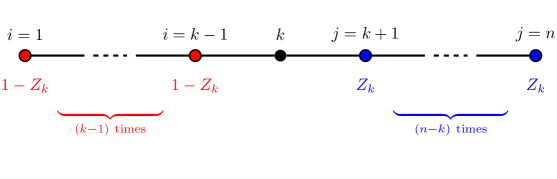
Figure 1. Display of the non-constant contributions to $\mathbb{E}(X_{\mathrm{inv}}\mid Z_{k})$

Proof.

We first study the conditional expectations $\mathbb{E}(X_{\mathrm{inv}}\mid Z_{k})$ for $k=1,\ldots,n$ and get

$$\mathbb{E}(X_{\mathrm{inv}}\mid Z_{k})=\sum_{1\leq i<j\leq n}\mathbb{P}(Z_{i}>Z_{j}\mid Z_{k})=\sum_{1\leq i<j\leq n}\begin{cases}1/2,&\text{ if }k\notin\{i,j\},\\ Z_{k},&\text{ if }k=i,\\ 1-Z_{k},&\text{ if }k=j.\end{cases}$$

We fix $k\in\{1,\ldots,n\}$ and analyze the frequency of the three cases on the right-hand side. As $\{1,\ldots,n\}\setminus\{k\}$ has cardinality $n-1,$ there are $\binom{n-1}{2}$ subsets $\{i,j\}\subseteq\{1,\ldots,n\}\setminus\{k\}$. When picking $i=k,$ there are $n-k$ indices $j$ with $j>k,$ for which we have $\mathbb{P}(Z_{k}>Z_{j}\mid Z_{k})=\mathbb{P}(Z_{j}<Z_{k}\mid Z_{k})=Z_{k}$ since $Z_{k}\sim U(0,1)$. Likewise, when picking $j=k,$ there are $k-1$ indices $i$ with $i<k,$ which gives $\mathbb{P}(Z_{i}>Z_{k}\mid Z_{k})=1-Z_{k}$. These contributions are illustrated in Figure 1. Therefore, we obtain

$$\mathbb{E}(X_{\mathrm{inv}}\mid Z_{k}) =\frac{1}{2}\binom{n-1}{2}+(n-k)Z_{k}+(k-1)(1-Z_{k})$$

$$=\frac{1}{2}\binom{n-1}{2}+(n-2k+1)Z_{k}+(k-1),$$

from which we deduce that

$$\hat{X}_{\mathrm{inv}} =\sum_{k=1}^{n}\mathbb{E}(X_{\mathrm{inv}}\mid Z_{k})-(n-1)\mathbb{E}(X_{\mathrm{inv}})$$

$$=\frac{n}{2}\binom{n-1}{2}+\sum_{k=1}^{n}(n-2k+1)Z_{k}+\sum_{k=1}^{n}(k-1)-\frac{n-1}{2}\binom{n}{2}$$

(4) $$=\frac{n(n-1)}{4}+\sum_{k=1}^{n}(n-2k+1)Z_{k}.$$

Since the $Z_{k}$’s are i.i.d. , the variance of the Hájek projection is

$$\mathrm{Var}(\hat{X}_{\mathrm{inv}})=\sum_{k=1}^{n}\mathrm{Var}((n-2k+1)Z_{k}).$$

Due to $\mathrm{Var}(Z_{k})=1/12,$ we get

$$\mathrm{Var}(\hat{X}_{\mathrm{inv}}) =\frac{1}{12}\sum_{k=1}^{n}(2k-n-1)^{2}=\frac{1}{12}\sum_{k=1}^{n}\bigl{(}4k^{2}+(n+1)^{2}-4k(n+1)\bigr{)}$$

$$=\frac{1}{12}\left(4\sum_{k=1}^{n}k^{2}+n(n+1)^{2}-4(n+1)\frac{n(n+1)}{2}\right)$$

$$=\frac{1}{12}\left(4\frac{n(n+1)(2n+1)}{6}-n(n+1)^{2}\right)=\frac{1}{36}n^{3}-\frac{n}{36}\,,\qquad n\to\infty.$$

By [18, Corollary 3.2], we have $\mathrm{Var}(X_{\mathrm{inv}})=\displaystyle{\frac{1}{36}n^{3}+\frac{9n^{2}+7n}{72}}$ and therefore $\mathrm{Var}(X_{\mathrm{inv}})\sim\mathrm{Var}(\hat{X}_{\mathrm{inv}})$ as $n\to\infty$. ∎

A combination of Theorem 2.2 and Lemma 2.3 yields

$$Y_{\mathrm{inv}}=\hat{Y}_{\mathrm{inv}}+o_{\mathbb{P}}(1)\,,\qquad n\to\infty\,.$$

Remark 2.4.

Interestingly, this approach fails for $X_{\mathrm{des}},$ since $\mathrm{Var}(X_{\mathrm{des}})\sim\mathrm{Var}(\hat{X}_{\mathrm{des}})$ does not hold. Repeating the considerations in the proof of Lemma 2.3 for $X_{\mathrm{des}},$ we first obtain

$$\mathbb{E}(X_{\mathrm{des}}\mid Z_{k})=\sum_{i=1}^{n-1}\mathbb{P}(Z_{i}>Z_{i+1}\mid Z_{k})=\sum_{i=1}^{n-1}\begin{cases}1/2,&k\notin\{i,i+1\},\\ Z_{k},&k=i,\\ 1-Z_{k},&k=i+1.\end{cases}$$

Now, except for the border cases $k=1$ and $k=n,$ the summands for $k=i$ and $k=i+1$ are each used exactly once, so the $Z_{k}$ in their sum $Z_{k}+(1-Z_{k})$ cancel out. In total, we obtain

$$\hat{X}_{\mathrm{des}}=Z_{1}-Z_{n}+c_{n}\,,$$

where $c_{n}$ is some constant that depends only on $n$. Therefore, $\mathrm{Var}(\hat{X}_{\mathrm{des}})=2/12$ does not have the linear order of $\mathrm{Var}(X_{\mathrm{des}})=(n+1)/12$ (see [18, Corollary 4.2]).

For these reasons, our results will be based on the following consequence of Theorem 2.2 and Lemma 2.3.

Corollary 2.5.

Let $(X_{\mathrm{inv}},X_{\mathrm{des}})^{\top}$ be given from the symmetric group $S_{n}$. For the standardized random vector $(Y_{\mathrm{inv}},Y_{\mathrm{des}})^{\top}$ and the standardized Hájek projection $\hat{Y}_{\mathrm{inv}}$, we have

$$\begin{pmatrix}Y_{\mathrm{inv}}\\ Y_{\mathrm{des}}\end{pmatrix}=\begin{pmatrix}\hat{Y}_{\mathrm{inv}}+o_{\mathbb{P}}(1)\\ Y_{\mathrm{des}}\end{pmatrix}.$$

A decomposition of $(\hat{X}_{\mathrm{inv}},X_{\mathrm{des}})^{\top}$ into $1$-dependent summands is given by

(5) $$\begin{pmatrix}\hat{X}_{\mathrm{inv}}\\ X_{\mathrm{des}}\end{pmatrix} =\sum_{k=1}^{n-1}\begin{pmatrix}(n-2k+1)Z_{k}\\ \mathbf{1}\{Z_{k}>Z_{k+1}\}\end{pmatrix}+\begin{pmatrix}-(n-1)Z_{n}+\frac{n(n-1)}{4}\\ 0\end{pmatrix}.$$

Likewise, a $1$-dependent decomposition for $(\hat{Y}_{\mathrm{inv}},Y_{\mathrm{des}})^{\top}$ can be found by standardization.

It is worth noting that the correlation $\mathrm{Corr}(X_{\mathrm{inv}},X_{\mathrm{des}})$ is not zero. However, we now show that $\mathrm{Corr}(X_{\mathrm{inv}},X_{\mathrm{des}})\to 0$ as $n\to\infty$. Moreover, by Corollary 2.5 the same holds true for $(\hat{X}_{\mathrm{inv}},X_{\mathrm{des}})^{\top}$ as well (in fact, $\mathrm{Corr}(\hat{X}_{\mathrm{inv}},X_{\mathrm{des}})$ is even easier to compute). To proceed, we need the covariance of $\hat{X}_{\mathrm{inv}}$ and $X_{\mathrm{des}}$. Our next result additionally provides $\mathrm{Cov}(X_{\mathrm{inv}},X_{\mathrm{des}})$, which – to the best of our knowledge – is not available in the literature.

Lemma 2.6 (see Subsections 8.1,  8.2 for the proof).

On the symmetric group $S_{n}$, we have

1. $\mathrm{Cov}(X_{\mathrm{inv}},X_{\mathrm{des}})=(n-1)/4$.

2. $\mathrm{Cov}(\hat{X}_{\mathrm{inv}},X_{\mathrm{des}})=(n-1)/6$.

Corollary 2.7.

Since $\mathrm{Var}(X_{\mathrm{inv}})\mathrm{Var}(X_{\mathrm{des}})=\Theta(n^{4})$ according to [18, Corollaries 3.2 and 4.2], and the same holds true if $\mathrm{Var}(X_{\mathrm{inv}})$ is replaced by $\mathrm{Var}(\hat{X}_{\mathrm{inv}}),$ we conclude from Lemma 2.6 that

$$\mathrm{Corr}(X_{\mathrm{inv}},X_{\mathrm{des}}) =\dfrac{\mathrm{Cov}(X_{\mathrm{inv}},X_{\mathrm{des}})}{\sqrt{\mathrm{Var}(X_{\mathrm{inv}})\mathrm{Var}(X_{\mathrm{des}})}}=\Theta(1/n)\,,$$

$$\mathrm{Corr}(\hat{X}_{\mathrm{inv}},X_{\mathrm{des}}) =\Theta(1/n)\,,\qquad n\rightarrow\infty.$$

3. The bivariate Central Limit Theorem

In this section, we establish the joint normality of $(X_{\mathrm{inv}},X_{\mathrm{des}})^{\top}$ by using the $1$-dependent decomposition of $(\hat{X}_{\mathrm{inv}},X_{\mathrm{des}})^{\top}$ and applying a recent (and quite optimized) CLT for $m$-dependent triangular arrays from Chang et al. [5]. Their work provides Gaussian approximations for high-dimensional data under various dependency frameworks, including $m$-dependence. It gives error rates over the system of all hyperrectangles, including the Kolmogorov distance as a special case. Moreover, the high-dimensional framework implicitly covers the finite-dimensional one by repeating the components of a vector.

Refining the notation of [5], we consider triangular arrays $(X_{t}^{(n)})_{t=1,\ldots,n}$ whose entries $X_{1}^{(n)},\ldots,X_{n}^{(n)}$ are mean zero random vectors in $\mathbb{R}^{\mathfrak{p}}$, where $\mathfrak{p}=\mathfrak{p}(n)$ can grow with respect to $n$. For the sum

(6) $$X^{(n)}:=\sum_{t=1}^{n}X_{t}^{(n)}\quad\text{ with covariance matrix }\Sigma^{(n)}:=\mathrm{Var}(X^{(n)}),$$

the work of Chang et al. [5] gives bounds and rates of convergence for

$$r_{n}(\mathcal{A}):=\sup_{A\in\mathcal{A}}|\mathbb{P}(X^{(n)}\in A)-\mathbb{P}(\mathcal{N}_{n}\in A)|,$$

where $\mathcal{A}$ encompasses a system of Borel sets and $\mathcal{N}_{n}\sim\mathrm{N}(0,\Sigma^{(n)})$ is a normal distribution with the same covariance structure as $X^{(n)}$. Bounds for $r_{n}(\mathcal{A})$ in both constant and high dimensions have been strongly investigated for independent variables. A seminal work for the system $\mathcal{A}:=\{[\textbf{x},\infty)\mid\textbf{x}\in\mathbb{R}^{\mathfrak{p}}\}$ to compare the maxima of $X^{(n)}$ and $\mathcal{N}_{n}$ in high dimensions is given by Chernozhukov et al. [7]. In recent years, there have been great efforts to improve the error bounds and the growth of dimension within the independent framework, see [8, 9, 12, 14, 19].

An interesting feature of [5] is that the $X_{t}^{(n)}$ are allowed to be dependent which offers a wide range of applications beyond the independent framework, including the $1$-dependent decomposition of $(\hat{X}_{\mathrm{inv}},X_{\mathrm{des}})^{\top}$. The following two conditions need to be imposed on the $X_{t}^{(n)}=(X_{t,1}^{(n)},\ldots,X_{t,\mathfrak{p}}^{(n)})^{\top}$.

Condition 1: There exists a sequence of constants $B_{n}\geq 1$ and a universal constant $\gamma_{1}\geq 1$ such that

$$\max_{j=1,\ldots,\mathfrak{p}}\mathbb{E}\left(\exp\left(\left|\sqrt{n}X_{t,j}^{(n)}\right|^{\gamma_{1}}B_{n}^{-\gamma_{1}}\right)\right)\leq 2\,,\qquad t=1,\ldots,n.$$

Condition 2: There exists a constant $K>0$ such that for all $n\in\mathbb{N}\negmedspace$

$$\min_{j=1,\ldots,\mathfrak{p}}\mathrm{Var}\left(\sum_{t=1}^{n}X_{t,j}^{(n)}\right)\geq K.$$

Remark 3.1.

Condition 1 means sub-Gaussianity, i.e., by Markov’s inequality,

$$\forall u>0\negmedspace:\quad\mathbb{P}(|\sqrt{n}X_{t,j}^{(n)}|>u)\leq 2\exp(-u^{\gamma_{1}}B_{n}^{-\gamma_{1}}).$$

For sub-Gaussian variables, particularly for the bounded variables $X_{\mathrm{des}},X_{\mathrm{inv}}$ and their Hájek projection $\hat{X}_{\mathrm{inv}}$, we can choose $\gamma_{1}=2$ and $B_{n}=O(1)$. Condition 2 implies non-degeneracy, which obviously holds true in our setting.

A very useful estimate of $r_{n}(\mathcal{A}^{\mathrm{re}})$ is given for the system of hyperrectangles

$$\mathcal{A}^{\mathrm{re}}:=\Bigl{\{}\{\textbf{w}\in\mathbb{R}^{\mathfrak{p}}\negmedspace:\textbf{a}\leq\textbf{w}\leq\textbf{b}\}\mid\textbf{a},\textbf{b}\in[-\infty,\infty]^{\mathfrak{p}}\Bigr{\}}.$$

Proposition 3.2 (see [5], Corollary 1).

Let $(X_{t}^{(n)})_{t=1,\ldots,n}$ be a triangular array of mean zero random vectors in high dimensions, i.e., $X_{1}^{(n)},\ldots,X_{n}^{(n)}\in\mathbb{R}^{\mathfrak{p}}$ with $\mathfrak{p}=\mathfrak{p}(n)\gg n^{\kappa}$ for a constant $\kappa>0$. Assume that each row $X_{1}^{(n)},\ldots,X_{n}^{(n)}$ is $m$-dependent with a global constant $m\in\mathbb{N}$. Under Conditions 1 and 2, it holds that

$$r_{n}(\mathcal{A}^{\mathrm{re}})=O\left(\frac{B_{n}m^{2/3}\log(\mathfrak{p})^{7/6}}{n^{1/6}}\right)\,,\qquad n\to\infty.$$

We note that if $\mathfrak{p}$ remains constant, we can artificially repeat the vector components (say $n$ times) and therefore, the requirement $\mathfrak{p}\gg n^{\kappa}$ can be removed. We obtain the following corollary.

Corollary 3.3.

Let $(X_{t}^{(n)})_{t=1,\ldots,n}$ be a triangular array of mean zero random vectors in fixed dimension $\mathfrak{p}$ and suppose that each row $X_{1}^{(n)},\ldots,X_{n}^{(n)}$ is $m$-dependent with a global constant $m\in\mathbb{N}$. Under Conditions 1 and 2, it holds that

$$r_{n}(\mathcal{A}^{\mathrm{re}})=O\left(\frac{B_{n}m^{2/3}\log(n)^{7/6}}{n^{1/6}}\right)\,,\qquad n\to\infty.$$

Our next result establishes a CLT for the joint distribution of inversions and descents.

Theorem 3.4.

The joint distribution of $(X_{\mathrm{inv}},X_{\mathrm{des}})^{\top}$ on the family of symmetric groups satisfies the CLT. This means

$$(Y_{\mathrm{inv}},Y_{\mathrm{des}})^{\top}=\left(\frac{X_{\mathrm{inv}}-\mathbb{E}(X_{\mathrm{inv}})}{\sqrt{\mathrm{Var}(X_{\mathrm{inv}})}},\frac{X_{\mathrm{des}}-\mathbb{E}(X_{\mathrm{des}})}{\sqrt{\mathrm{Var}(X_{\mathrm{des}})}}\right)^{\top}\overset{\mathcal{D}}{\longrightarrow}\mathrm{N}_{2}(0,\mathrm{I}_{2})\,,\qquad n\to\infty.$$

Proof.

Due to Corollary 2.5 and Slutsky’s Theorem, it suffices to show that $(\hat{Y}_{\mathrm{inv}},Y_{\mathrm{des}})^{\top}\overset{\mathcal{D}}{\longrightarrow}\mathrm{N}_{2}(0,\mathrm{I}_{2})$. By (5), we have that

(7) $$\begin{pmatrix}\hat{X}_{\mathrm{inv}}-\mathbb{E}(\hat{X}_{\mathrm{inv}})\\ X_{\mathrm{des}}-\mathbb{E}(X_{\mathrm{des}})\end{pmatrix} =\sum_{k=1}^{n-1}\begin{pmatrix}(n-2k+1)(Z_{k}-1/2)\\ \mathbf{1}\{Z_{k}>Z_{k+1}\}-1/2\end{pmatrix}+\begin{pmatrix}-(n-1)(Z_{n}-1/2)\\ 0\end{pmatrix}$$

is a sum of $1$-dependent random vectors with mean zero. Setting

$$X_{k}^{(n)} :=\begin{pmatrix}(n-2k+1)(Z_{k}-1/2)/\sqrt{\mathrm{Var}(\hat{X}_{\mathrm{inv}})}\\ (\mathbf{1}\{Z_{k}>Z_{k+1}\}-1/2)/\sqrt{\mathrm{Var}(X_{\mathrm{des}})}\end{pmatrix},\qquad k=1,\ldots,n-1,$$

$$X_{n}^{(n)} :=\begin{pmatrix}-(n-1)(Z_{n}-1/2)/\sqrt{\mathrm{Var}(\hat{X}_{\mathrm{inv}})}\\ 0\end{pmatrix},$$

we obtain the representation $(\hat{Y}_{\mathrm{inv}},Y_{\mathrm{des}})^{\top}=\sum_{k=1}^{n}X_{k}^{(n)}=:X^{(n)}$. The covariance matrix of $X^{(n)}$ (see (6)) is given by $\Sigma^{(n)}=\begin{pmatrix}1&\rho_{n}\\ \rho_{n}&1\end{pmatrix}$, where $\rho_{n}:=\mathrm{Corr}(\hat{X}_{\mathrm{inv}},X_{\mathrm{des}})$. An application of Corollary 3.3 yields that for $\mathcal{N}_{n}\sim\mathrm{N}(0,\Sigma^{(n)})$,

$$\sup_{u\in\mathbb{R}^{2}}|\mathbb{P}(X^{(n)}\leq u)-\mathbb{P}(\mathcal{N}_{n}\leq u)| \leq r_{n}(\mathcal{A}^{\text{re}})=O\left(n^{-1/6}\log(n)^{7/6}\right)\,.$$

In combination with the fact that the correlation $\rho_{n}$ vanishes in the limit (see Corollary 2.7), we can conclude that $(\hat{Y}_{\mathrm{inv}},Y_{\mathrm{des}})^{\top}\overset{\mathcal{D}}{\longrightarrow}\mathrm{N}_{2}(0,\mathrm{I}_{2})$, completing the proof of the theorem. ∎

4. The Extreme Value Limit Theorem

In what follows, we use the Gaussian approximation of Proposition 3.2 to prove that the vector of componentwise maxima of i.i.d. copies of $(X_{\mathrm{inv}},X_{\mathrm{des}})^{\top}$ is attracted to the bivariate Gumbel distribution with independent margins. First, we briefly recapitulate the procedure used in [13] for the univariate case. Let $(k_{n})_{n\in\mathbb{N}}$ be a divergent sequence of positive integers. It is well known (see, e.g., [20, Theorem 1.5.3]) that the maximum of $k_{n}$ i.i.d. standard normal variables $(N_{i})_{i=1,\ldots,k_{n}}$ is attracted toward the standard Gumbel distribution $\Lambda(x)=\exp(-\exp(-x))$ by virtue of

$$\alpha_{n}\big{(}\max\{N_{1},\ldots,N_{k_{n}}\}-\alpha_{n}\big{)}\overset{\mathcal{D}}{\longrightarrow}\Lambda,\qquad n\to\infty,$$

where

$$\alpha_{n}:=\sqrt{2\log k_{n}}-\frac{\log\log k_{n}+\log(4\pi)}{2\sqrt{2\log k_{n}}}.$$

The key step in the results of [13] was to employ large deviations theory in order to establish the tail equivalence

$$\mathbb{P}\big{(}X/\sqrt{\mathrm{Var}(X)}>x_{n}\big{)}\sim 1-\Phi(x_{n}),\qquad n\to\infty\,,$$

where $X$ denotes the centered version of either $X_{\mathrm{inv}}$ or $X_{\mathrm{des}}$ on $S_{n}$, and $\Phi$ is the standard normal distribution function and $x_{n}\to\infty$ is a suitable sequence of real numbers. In the multivariate case, we additionally need to control the dependence between $X_{\mathrm{inv}}$ and $X_{\mathrm{des}}$ which we facilitate by Proposition 3.2 after first replacing $X_{\mathrm{inv}}$ with its Hájek projection $\hat{X}_{\mathrm{inv}}$.

Let $(X_{\mathrm{inv}}^{(j)},X_{\mathrm{des}}^{(j)})^{\top},j=1,\ldots,k_{n}$ be independent copies of $(X_{\mathrm{inv}},X_{\mathrm{des}})^{\top}$ on $S_{n}$. We are interested in the asymptotic joint distribution of the component-wise maxima of $(X_{\mathrm{inv}},X_{\mathrm{des}})^{\top}$. Equivalently, we investigate the standardized maxima

(8) $$M_{n,\mathrm{inv}} :=\frac{\max_{j=1,\ldots,k_{n}}X_{\mathrm{inv}}^{(j)}-\mathbb{E}(X_{\mathrm{inv}})}{\sigma(X_{\mathrm{inv}})}\quad\text{ and }\quad M_{n,\mathrm{des}}:=\frac{\max_{j=1,\ldots,k_{n}}X_{\mathrm{des}}^{(j)}-\mathbb{E}(X_{\mathrm{des}})}{\sigma(X_{\mathrm{des}})}\,.$$

We now postulate the main result of this paper. If the number of samples $k_{n}$ is not too large, then the distribution of $(X_{\mathrm{inv}},X_{\mathrm{des}})^{\top}$ is in the maximum domain of attraction of a bivariate Gumbel distribution with independent margins.

Theorem 4.1.

Consider the setting from above and assume $(k_{n}\log k_{n})/n\to 0$ as $n\to\infty$. Then, it holds that

(9) $$\lim_{n\to\infty}{\mathbb{P}}\big{(}\alpha_{n}(M_{n,\mathrm{inv}}-\alpha_{n})\leq x,\alpha_{n}(M_{n,\mathrm{des}}-\alpha_{n})\leq y\big{)}=\Lambda(x)\Lambda(y)\,,\qquad x,y\in\mathbb{R}\,.$$

In particular, the maxima of inversions and descents on $S_{n}$ are asymptotically independent.

Proof.

Let $(Z_{i}^{j})_{i,j\geq 1}$ be a collection of independent $U(0,1)$ distributed random variables and recall that $\alpha_{n}\sim\sqrt{2\log k_{n}}$. Then we have the representation

$$\begin{pmatrix}X_{\mathrm{inv}}^{(j)}\\ X_{\mathrm{des}}^{(j)}\end{pmatrix}_{j=1,\ldots,k_{n}}\stackrel{{\scriptstyle\mathcal{D}}}{{=}}\begin{pmatrix}\sum_{1\leq i<k\leq n}\textbf{1}\{Z_{i}^{(j)}>Z_{k}^{(j)}\}\\ \sum_{i=1}^{n-1}\textbf{1}\{Z_{i}^{(j)}>Z_{i+1}^{(j)}\}\end{pmatrix}_{j=1,\ldots,k_{n}}.$$

Therefore, by Slutsky’s theorem, (9) is an immediate consequence of

(10) $$\lim_{n\to\infty}{\mathbb{P}}\big{(}\alpha_{n}(\hat{M}_{n}-\alpha_{n})\leq x,\alpha_{n}(M_{n,\mathrm{des}}-\alpha_{n})\leq y\big{)}=\Lambda(x)\Lambda(y)\,,\qquad x,y\in\mathbb{R}\,,$$

and

(11) $$\sqrt{\log k_{n}}\,|M_{n,\mathrm{inv}}-\hat{M}_{n}|\overset{\mathbb{P}}{\longrightarrow}0\,,\qquad n\to\infty\,,$$

where $\hat{M}_{n}:=\sigma(\hat{X}_{\mathrm{inv}})^{-1}\left(\max_{j=1,\ldots,k_{n}}\hat{X}_{\mathrm{inv}}^{(j)}-\mathbb{E}(X_{\mathrm{inv}})\right)$. It remains to show (10) and (11). We begin with the proof of (11) and get

$$|M_{n,\mathrm{inv}}-\hat{M}_{n}| \leq\max_{j=1,\ldots,k_{n}}\bigg{|}\frac{X_{\mathrm{inv}}^{(j)}-\mathbb{E}(X_{\mathrm{inv}})}{\sigma(X_{\mathrm{inv}})}-\frac{\hat{X}_{\mathrm{inv}}^{(j)}-\mathbb{E}(X_{\mathrm{inv}})}{\sigma(\hat{X}_{\mathrm{inv}})}\bigg{|}$$

$$=\max_{j=1,\ldots,k_{n}}\bigg{|}\frac{X_{\mathrm{inv}}^{(j)}-\hat{X}_{\mathrm{inv}}^{(j)}}{\sigma(X_{\mathrm{inv}})}+(\hat{X}_{\mathrm{inv}}^{(j)}-\mathbb{E}(X_{\mathrm{inv}}))\frac{\sigma(\hat{X}_{\mathrm{inv}})-\sigma(X_{\mathrm{inv}})}{\sigma(X_{\mathrm{inv}})\sigma(\hat{X}_{\mathrm{inv}})}\bigg{|}\,.$$

Thus, for any $\varepsilon>0$, we obtain

$${\mathbb{P}}\Big{(}\sqrt{\log k_{n}}\,|M_{n,\mathrm{inv}}-\hat{M}_{n}|>2\varepsilon\Big{)}\leq{\mathbb{P}}\Big{(}\sqrt{\log k_{n}}\max_{j=1,\ldots,k_{n}}\bigg{|}\frac{X_{\mathrm{inv}}^{(j)}-\hat{X}_{\mathrm{inv}}^{(j)}}{\sigma(X_{\mathrm{inv}})}\bigg{|}>\varepsilon\Big{)}$$

$$+{\mathbb{P}}\Big{(}\sqrt{\log k_{n}}\max_{j=1,\ldots,k_{n}}\bigg{|}(\hat{X}_{\mathrm{inv}}^{(j)}-\mathbb{E}(X_{\mathrm{inv}}))\frac{\sigma(\hat{X}_{\mathrm{inv}})-\sigma(X_{\mathrm{inv}})}{\sigma(X_{\mathrm{inv}})\sigma(\hat{X}_{\mathrm{inv}})}\bigg{|}>\varepsilon\Big{)}=:P_{1}+P_{2}\,.$$

Using the union bound and Markov’s inequality, we have

$$P_{1} \leq k_{n}\,{\mathbb{P}}\Big{(}|X_{\mathrm{inv}}-\hat{X}_{\mathrm{inv}}|>\frac{\sigma(X_{\mathrm{inv}})\varepsilon}{\sqrt{\log k_{n}}}\Big{)}\leq k_{n}\,\frac{\log k_{n}}{\mathrm{Var}(X_{\mathrm{inv}})\varepsilon^{2}}\mathbb{E}|X_{\mathrm{inv}}-\hat{X}_{\mathrm{inv}}|^{2}$$

$$=\frac{k_{n}\log k_{n}}{\mathrm{Var}(X_{\mathrm{inv}})\varepsilon^{2}}\Big{(}\mathrm{Var}(X_{\mathrm{inv}})+\mathrm{Var}(\hat{X}_{\mathrm{inv}})-2\mathrm{Cov}(X_{\mathrm{inv}},\hat{X}_{\mathrm{inv}})\Big{)}$$

(12) $$=\frac{k_{n}\log k_{n}}{\varepsilon^{2}}\Big{(}1-\frac{\mathrm{Var}(\hat{X}_{\mathrm{inv}})}{\mathrm{Var}(X_{\mathrm{inv}})}\Big{)}\,,$$

where the last equality follows from the fact that $\mathrm{Cov}(X_{\mathrm{inv}},\hat{X}_{\mathrm{inv}})=\mathrm{Var}(\hat{X}_{\mathrm{inv}})$, see, e.g., [24, Theorem 11.1]. Plugging in the formulas for $\mathrm{Var}(X_{\mathrm{inv}})$ and $\mathrm{Var}(\hat{X}_{\mathrm{inv}})$ from the end of the proof of Lemma 2.3, we get $\mathrm{Var}(\hat{X}_{\mathrm{inv}})/\mathrm{Var}(X_{\mathrm{inv}})=1+O(1/n)$ from which we conclude that

$$P_{1}=k_{n}\log k_{n}\,O(1/n)\,,\qquad n\to\infty\,,$$

which tends to zero by the assumption on $k_{n}$. Repeating the above considerations for $P_{2}$ yields

$$P_{2} \leq\frac{k_{n}\log k_{n}}{\varepsilon^{2}}\Big{(}\frac{\sigma(\hat{X}_{\mathrm{inv}})-\sigma(X_{\mathrm{inv}})}{\sigma(X_{\mathrm{inv}})}\Big{)}^{2}\mathbb{E}\Big{(}\frac{\hat{X}_{\mathrm{inv}}^{(j)}-\mathbb{E}(X_{\mathrm{inv}})}{\sigma(\hat{X}_{\mathrm{inv}})}\Big{)}^{2}$$

(13) $$=k_{n}\log k_{n}\,O(1/n)=o(1)\,,\qquad n\to\infty\,,$$

which completes the proof of (11). Regarding (10), we recall that by Corollary 2.5,

$$\begin{pmatrix}\hat{X}_{\mathrm{inv}}^{(j)}-\mathbb{E}(\hat{X}_{\mathrm{inv}}^{(j)})\\ X_{\mathrm{des}}^{(j)}-\mathbb{E}(X_{\mathrm{des}}^{(j)})\end{pmatrix} =\sum_{k=1}^{n-1}\begin{pmatrix}(n-2k+1)(Z_{k}^{(j)}-1/2)\\ \mathbf{1}\{Z_{k}^{(j)}>Z_{k+1}^{(j)}\}-1/2\end{pmatrix}+\begin{pmatrix}-(n-1)(Z_{n}^{(j)}-1/2)\\ 0\end{pmatrix}.$$

This is a sum of 1-dependent centered random vectors. Setting

$$Y_{k}^{(n,j)} :=\begin{pmatrix}(n-2k+1)(Z_{k}^{(j)}-1/2)/\sigma(\hat{X}_{\mathrm{inv}})\\ (\mathbf{1}\{Z_{k}^{(j)}>Z_{k+1}^{(j)}\}-1/2)/\sigma(X_{\mathrm{des}})\end{pmatrix},\qquad k=1,\ldots,n-1,$$

$$Y_{n}^{(n,j)} :=\begin{pmatrix}-(n-1)(Z_{n}^{(j)}-1/2)/\sigma(\hat{X}_{\mathrm{inv}})\\ 0\end{pmatrix},$$

we obtain the representation $(\hat{Y}_{\mathrm{inv}}^{(j)},Y_{\mathrm{des}}^{(j)})^{\top}=\sum_{k=1}^{n}Y_{k}^{(n,j)}$. The covariance matrix of $(\hat{Y}_{\mathrm{inv}}^{(j)},Y_{\mathrm{des}}^{(j)})^{\top}$ is given by $\Sigma^{(n)}=\begin{pmatrix}1&\rho_{n}\\ \rho_{n}&1\end{pmatrix}$, where $\rho_{n}:=\mathrm{Corr}(\hat{X}_{\mathrm{inv}},X_{\mathrm{des}})$. For a centered normal random vector $\mathcal{N}_{n}=(N_{1},\ldots,N_{2k_{n}})^{\top}$ whose covariance matrix is block-diagonal with all $k_{n}$ diagonal blocks equal to $\Sigma^{(n)}$, we write

$$P_{n}(x,y):={\mathbb{P}}\left(\alpha_{n}\Big{(}\max_{j=1,\ldots,k_{n}}N_{2j-1}-\alpha_{n}\Big{)}\leq x,\alpha_{n}\Big{(}\max_{j=1,\ldots,k_{n}}N_{2j}-\alpha_{n}\Big{)}\leq y\right)\,,\qquad x,y\in\mathbb{R}\,.$$

An application of Proposition 3.2 then yields, as $n\to\infty$,

$$\big{|}{\mathbb{P}}\big{(}\alpha_{n}(\hat{M}_{n}-\alpha_{n})\leq x,\alpha_{n}(M_{n,\mathrm{des}}-\alpha_{n})\leq y\big{)}-P_{n}(x,y)\big{|}$$

$$=O\left(n^{-1/6}\log(\max\{n,k_{n}\})^{7/6}\right)=o(1)\,.$$

Finally, since $\rho_{n}\to 0$ (see Corollary 2.7), it is a standard result for maxima of bivariate Gaussian random vectors (with correlation strictly less than $1$) that

$$P_{n}(x,y)\overset{n\rightarrow\infty}{\longrightarrow}\Lambda(x)\Lambda(y),$$

completing the proof of (10). ∎

Remark 4.2.

The upper bound for the row-wise number of samples $k_{n}$ is stricter than that for the individual statistics $X_{\mathrm{inv}}$ and $X_{\mathrm{des}}$ given in [13], due to the error that arises from replacing $X_{\mathrm{inv}}$ with $\hat{X}_{\mathrm{inv}}$. In particular, this excludes the choice of $k_{n}=n$ which gives a uniformly stretched triangular array. On the other hand, this new EVLT can be transferred to other individual and joint permutation statistics, since it is mainly based on a Gaussian approximation for $m$-dependent random vectors (or variables). Besides descents, some other examples of $m$-dependent permutation statistics on $S_{n}$ are peaks (all indices $i$ with $\pi(i-1)<\pi(i)>\pi(i+1)$) and valleys (all $i$ with $\pi(i-1)>\pi(i)<\pi(i+1)$). Since the proof of Theorem 4.1 does not rely on any special property of descents other than $m$-dependence, any other $m$-dependent permutation statistic could be combined with inversions.

Furthermore, if we consider a permutation statistic consisting of one or two $m$-dependent components, then there is no need to use Hájek’s projection and the corresponding part in the proof of Theorem 4.1 can be removed. In this case, only (10) needs to be shown and the upper bound of $k_{n}$ only comes from

$$n^{-1/6}\log(k_{n})^{7/6}=o(1)\Longleftrightarrow k_{n}=\exp\big{(}o(n^{1/7})\big{)}.$$

Therefore, in this situation, Theorem 4.1 can be modified to give almost the same flexibility as [13, Theorem 4.2].

5. Signed and even-signed permutation groups

The previous two sections established the CLT and the EVLT for the joint distribution $(X_{\mathrm{inv}},X_{\mathrm{des}})^{\top}$ on the family of symmetric groups. We now work toward these results for $(X_{\mathrm{inv}},X_{\mathrm{des}})^{\top}$ on the signed and even-signed permutation groups $B_{n}$ and $D_{n}$ that generalize the symmetric groups $S_{n}$.

The group $B_{n}$ of signed permutations on $n$ letters arises from $S_{n}$ by assigning any combination of positive or negative signs to the entries of a permutation. The even-signed permutation group $D_{n}$ is the subgroup of $B_{n}$ consisting of elements with an even number of negative signs. As in [18, Section 2.1], we use the in-line notation

$$B_{n}=\bigl{\{}\pi=(\pi(1),\ldots,\pi(n)):~{} \pi(i)\in\{\pm 1,\ldots,\pm n\}~{}\forall i,$$

(14) $$\{|\pi(1)|,\ldots,|\pi(n)|\}=\{1,\ldots,n\}\bigr{\}},$$

and we have $D_{n}=\{\pi\in B_{n}\negmedspace:\pi(1)\pi(2)\cdots\pi(n)>0\}$.

According to [18], the combinatorial representation of inversions on $B_{n}$ and $D_{n}$ is given by

(15) $$\mathrm{Inv}(\pi)=\begin{cases}\mathrm{Inv}^{+}(\pi)\cup\mathrm{Inv}^{-}(\pi)\cup\mathrm{Inv}^{\circ}(\pi),&\text{ if }\pi\in B_{n},\\ \mathrm{Inv}^{+}(\pi)\cup\mathrm{Inv}^{-}(\pi)\,,&\text{ if }\pi\in D_{n}\,,\end{cases}$$

for the disjoint sets

$$\mathrm{Inv}^{+}(\pi) =\{1\leq i<j\leq n\mid\pi(i)>\pi(j)\},$$

$$\mathrm{Inv}^{-}(\pi) =\{1\leq i<j\leq n\mid-\pi(i)>\pi(j)\},$$

$$\mathrm{Inv}^{\circ}\hskip 2.41849pt(\pi) =\{1\leq i\leq n\mid\pi(i)<0\}.$$

Thus, the numbers of inversions on $B_{n}$ and $D_{n}$ are

$$X_{\mathrm{inv}}^{B}(\pi) =|\mathrm{Inv}^{+}(\pi)|+|\mathrm{Inv}^{-}(\pi)|+|\mathrm{Inv}^{\circ}(\pi)|,$$

$$X_{\mathrm{inv}}^{D}(\pi) =|\mathrm{Inv}^{+}(\pi)|+|\mathrm{Inv}^{-}(\pi)|.$$

The set $\mathrm{Inv}^{+}$ is analogous to inversions on symmetric groups. Note that on $B_{n}$ and $D_{n}$, one must pay attention to signs, that means, a pair $(i,j)$ with $\pi(i),\pi(j)<0$ and $|\pi(i)|<|\pi(j)|$ also adds to $\mathrm{Inv}^{+}(\pi)$. The set $\mathrm{Inv}^{-}$ is that of negative sum pairs. The set $\mathrm{Inv}^{\circ}(\pi)$ simply collects positions with negative entries. The latter two sets need to be counted so that $|\mathrm{Inv}(\pi)|$ equals the word length on $B_{n}$ with respect to the generating system $\{s_{0},s_{1},\ldots,s_{n-1}\},$ where $s_{0}=(-1,2,3,\ldots,n)$ negates the first entry and $s_{i}=(1,\ldots,i-1,i+1,i,i+2,\ldots,n)$ is the transposition of $i$ and $i+1$. The group $D_{n}$ is generated by $\{\tilde{s}_{0},s_{1},\ldots,s_{n-1}\}$ with $\tilde{s}_{0}=(-2,-1,3,\ldots,n)$, thus it is sufficient to add only $|\mathrm{Inv}^{-}(\pi)|$ to $|\mathrm{Inv}^{+}(\pi)|$. For more details and formal proofs, see [3, Sections 8.1 and 8.2].

The knowledge of generating systems also allows to derive simple representations of $X_{\mathrm{des}}$ on $B_{n}$ and $D_{n}$. Expand the in-line notation in (14) by setting $\pi(0):=0$. Then, according to [3, Sections 8.1 and 8.2],

(16a) $$X_{\mathrm{des}}^{B}(\pi)=\sum_{i=0}^{n-1}\textbf{1}\{\pi(i)>\pi(i+1)\},$$

and on the even-signed permutation group $$D_{n}$$,

(16b) $$X_{\mathrm{des}}^{D}(\pi)=\textbf{1}\{-\pi(2)>\pi(1)\}+\sum_{i=1}^{n-1}\textbf{1}\{\pi(i)>\pi(i+1)\}.$$

To draw elements uniformly from $B_{n}$, one can first draw some uniform $\pi\in S_{n}$ and then multiply each $\pi(i)$ with a Rademacher variable independent of everything else. Instead of the Rademacher variables, we propose a more general approach by drawing signs with a fixed $p$-bias, i.e., each sign is $-1$ with probability $p\in[0,1]$ and $+1$ with probability $q:=1-p$. This yields a family of probability measures on $B_{n}$, where the case $p=1/2$ corresponds to the uniform distribution on $B_{n}$, while if $p=0$, all mass is on the symmetric group $S_{n}\subset B_{n}$.

A corresponding probability distribution on the even-signed permutation group $D_{n}$ is obtained by first choosing the unsigned permutation $|\pi|\in S_{n}$ uniformly and then assigning $n-1$ signs for the entries $\pi(1),\ldots,\pi(n-1)$ with $p$-bias, and finally specifying the sign of $\pi(n)$ such that $\pi(1)\cdots\pi(n-1)\pi(n)>0$.

Definition 5.1.

Let $p\in[0,1]$ and $q:=1-p$. Then, the $p$-biased signed permutations measure on the group $B_{n}$ is the probability measure induced by the point masses

$$\mathbb{P}(\{\pi\})=\frac{1}{n!}p^{\text{neg}(\pi)}q^{n-\text{neg}(\pi)},\qquad\pi\in B_{n}\,,$$

where $\text{neg}(\pi)$ denotes the number of negative signs in $\pi$ and we use the convention $0^{0}:=1$. The $p$-biased signed permutations measure on $D_{n}$ is derived as described above.

Therefore, the entries of $\pi$, with $\pi$ distributed according to the $p$-biased signed permutations measure, can be represented by i.i.d. random variables $Z_{1},\ldots,Z_{n}$ with $\forall i=1,\ldots,n\negmedspace:Z_{i}=U_{i}R_{i},$ where $R_{i}$ is a $\pm 1$-valued random variable with

$$\mathbb{P}(R_{i}=-1)=p\quad\text{ and }\quad\mathbb{P}(R_{i}=1)=q,$$

and $U_{i}\sim U(0,1)$ is independent of $R_{i}$. The probability distribution function of $Z_{1}$ is

$$F_{p}(z):={\mathbb{P}}(Z_{1}\leq z)=\begin{cases}pz+p,&\quad z\in[-1,0],\\ qz+p,&\quad z\in[0,1],\end{cases}$$

and we simply write $Z_{1}\sim\mathrm{GR}(p)$ (generalized Rademacher with parameter $p$). Note the special cases $\mathrm{GR}(0)=U(0,1),$ $\mathrm{GR}(1/2)=U(-1,1)$ and $\mathrm{GR}(1)=U(-1,0)$. Figure 2 illustrates $F_{p}$ in the cases of $p=0,p=1/4$ and $p=3/4$. Accordingly, the Lebesgue density of $\mathrm{GR}(p)$ is $f_{p}(z)=p\textbf{1}\{-1<z<0\}+q\textbf{1}\{0<z<1\}$.

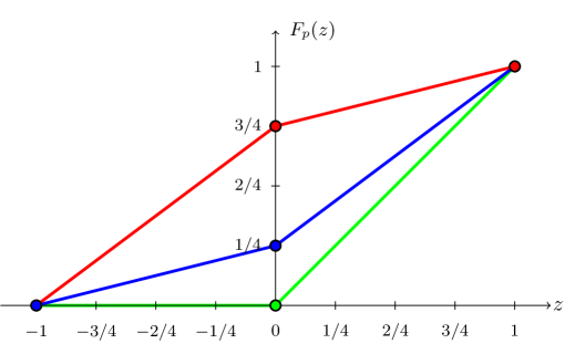
Figure 2. Probability distribution functions of $\mathrm{GR}(p)$ for $p=0$ (green), $p=1/4$ (blue) and $p=3/4$ (red).

Remark 5.2.

Let $X_{\mathrm{inv}}^{B}$ denote the random number of inversions on $B_{n}$ and let $X_{\mathrm{inv}}^{D}$ denote that on $D_{n}$. According to (15), we can write

(17a) $$X_{\mathrm{inv}}^{B} =\sum_{i<j}\textbf{1}\{Z_{i}>Z_{j}\}+\sum_{i<j}\textbf{1}\{-Z_{i}>Z_{j}\}+\sum_{i=1}^{n}\textbf{1}\{Z_{i}<0\},$$

(17b) $$X_{\mathrm{inv}}^{D} =\sum_{i<j}\textbf{1}\{Z_{i}>Z_{j}\}+\sum_{i<j}\textbf{1}\{-Z_{i}>Z_{j}\}.$$

Furthermore, (16a) and (16b) translate to

(18a) $$X_{\mathrm{des}}^{B} =\sum_{i=1}^{n-1}\textbf{1}\{Z_{i}>Z_{i+1}\}+\textbf{1}\{Z_{1}<0\},$$

(18b) $$X_{\mathrm{des}}^{D} =\sum_{i=1}^{n-1}\textbf{1}\{Z_{i}>Z_{i+1}\}+\textbf{1}\{-Z_{2}>Z_{1}\}.$$

In what follows, we use $X_{\mathrm{inv}}$ and $X_{\mathrm{des}}$ as an umbrella notation for the numbers of inversions and descents on each of the groups $S_{n},B_{n}$ and $D_{n}$. Again, both (18a) and (18b) give a $1$-dependent representation of $X_{\mathrm{des}}$, which yields a $1$-dependent representation of $(\hat{X}_{\mathrm{inv}},X_{\mathrm{des}})^{\top}$.

In the uniform case ($p=1/2$), the means and variances are known by [18, Corollaries 3.2 and 4.2]. We now calculate them within the general $p$-bias framework. To this end, we first observe that for any $i<j$,

$${\mathbb{P}}(-Z_{i}>Z_{j}) =\mathbb{E}({\mathbb{P}}(-Z_{i}>Z_{j}|Z_{i}))=\mathbb{E}(F_{p}(-Z_{i}))=\mathbb{E}(\mathbb{E}(F_{p}(-Z_{i})|U_{i}))$$

$$=\mathbb{E}(pF_{p}(U_{i})+qF_{p}(-U_{i}))=\mathbb{E}(p(qU_{i}+p)+q(-pU_{i}+p))=p\,.$$

Then, it follows straightforwardly from (17a) and (17b) that

$$\mathbb{E}\left(X_{\mathrm{inv}}^{B}\right) =\binom{n}{2}\left(p+\frac{1}{2}\right)+np, \mathbb{E}\left(X_{\mathrm{inv}}^{D}\right) =\binom{n}{2}\left(p+\frac{1}{2}\right).$$

The formula for $\mathrm{Var}(X_{\mathrm{inv}})$ is given in the next lemma.

Lemma 5.3 (see Subsection 8.3 for the proof).

On the $p$-biased (even-)signed permutation groups, we have

$$\mathrm{Var}\left(X_{\mathrm{inv}}^{B}\right) =\left(-\frac{1}{3}p^{2}+\frac{1}{3}p+\frac{1}{36}\right)n^{3}-\left(3p^{3}-4p^{2}+p-\frac{1}{24}\right)n^{2}$$

$$\hskip 5.69054pt\qquad+~{}\left(3p^{3}-\frac{14}{3}p^{2}+\frac{5}{3}p-\frac{5}{72}\right)n,$$

$$\mathrm{Var}\left(X_{\mathrm{inv}}^{D}\right) =\left(-\frac{1}{3}p^{2}+\frac{1}{3}p+\frac{1}{36}\right)n^{3}-\left(p^{3}-2p^{2}+p-\frac{1}{24}\right)n^{2}$$

$$\hskip 5.69054pt\qquad+~{}\left(p^{3}-\frac{5}{3}p^{2}+\frac{2}{3}p-\frac{5}{72}\right)n.$$

In particular, if $p=0$ or $p=1/2,$ we obtain the results in [18, Corollaries 3.2 and 4.2].

For the variance of $\hat{X}_{\mathrm{inv}}$ on $B_{n}$ and $D_{n}$, we get the same leading term as in Lemma 5.3, regardless of $p$. Hence, we obtain the Hájek approximation statement from Lemma 2.3 on the groups $B_{n}$ and $D_{n}$ with $p$-bias.

Lemma 5.4 (see Subsection 8.4 for the proof).

On the $p$-biased (even-)signed permutation groups, we also have

$$\mathrm{Var}(\hat{X}_{\mathrm{inv}})=\left(-\frac{1}{3}p^{2}+\frac{1}{3}p+\frac{1}{36}\right)n^{3}+O(n^{2}),$$

so $\hat{Y}_{\mathrm{inv}}=Y_{\mathrm{inv}}+o_{\mathbb{P}}(1)$ applies according to Theorem 2.2.

The leading term, as a function of $p$, has no zeros in $[0,1]$ and assumes its global maximum at $p=1/2,$ which is the unbiased case. This means that the order of $\mathrm{Var}(X_{\mathrm{inv}})$ and $\mathrm{Var}(\hat{X}_{\mathrm{inv}})$ is guaranteed to be cubic in $n$.

From Lemma 5.4, we obtain an extension of Corollary 2.5, which we present as a general statement on all three families of classical Weyl groups.

Corollary 5.5.

Let $W$ be a classical Weyl group of rank $n$, that is, $W\in\{S_{n},B_{n},D_{n}\}$. Set $Z_{0}:=-\infty$ if $W=S_{n}$, $Z_{0}:=0$ if $W=B_{n}$ and $Z_{0}:=-Z_{2}$ if $W=D_{n}$. Then,

$$\begin{pmatrix}\!\hat{X}_{\mathrm{inv}}\!\\ \!X_{\mathrm{des}}\!\end{pmatrix} \!=\!\begin{pmatrix}\mathbb{E}(X_{\mathrm{inv}}\mid Z_{1})\\ \mathbf{1}\{Z_{0}>Z_{1}\}\end{pmatrix}+\ldots+\begin{pmatrix}\mathbb{E}(X_{\mathrm{inv}}\mid Z_{n-1})\\ \mathbf{1}\{Z_{n-2}>Z_{n-1}\}\end{pmatrix}+\begin{pmatrix}\mathbb{E}(X_{\mathrm{inv}}\mid Z_{n})\!-\!(n\!-\!1)\mathbb{E}(X_{\mathrm{inv}})\\ \mathbf{1}\{Z_{n-1}>Z_{n}\}\end{pmatrix}$$

is a $1$-dependent decomposition of $(\hat{X}_{\mathrm{inv}},X_{\mathrm{des}})^{\top}$. On $B_{n}$ and $D_{n}$, this applies with any sign bias.

Lemma 5.6 (see Subsections 8.5, 8.6 for the proof).

On both of the groups $B_{n}$ and $D_{n}$ with $p$-bias, it holds that

1. $\mathrm{Corr}(X_{\mathrm{inv}},X_{\mathrm{des}})\longrightarrow 0$ as $n\to\infty$, and

   $$\mathrm{Cov}(X_{\mathrm{inv}}^{B},X_{\mathrm{des}}^{B}) =(n-1)\left(\frac{p^{2}}{2}+p^{2}q-\frac{p}{2}+\frac{1}{4}\right)+(p-p^{2}),$$

   $$\mathrm{Cov}(X_{\mathrm{inv}}^{D},X_{\mathrm{des}}^{D}) =(n-1)\left(\frac{p^{2}}{2}+p^{2}q-\frac{p}{2}+\frac{1}{4}\right)+p^{2}.$$

2. $\mathrm{Cov}(\hat{X}_{\mathrm{inv}},X_{\mathrm{des}})=\Theta(1/n),$ so again, $\mathrm{Corr}(\hat{X}_{\mathrm{inv}},X_{\mathrm{des}})\longrightarrow 0$ as $n\to\infty$.

The CLT of $(X_{\mathrm{inv}},X_{\mathrm{des}})^{\top}$ on $B_{n}$ and $D_{n}$ is now derived analogously to Theorem 3.4. Likewise, all arguments in the proof of the extreme value limit Theorem 4.1 apply on $B_{n}$ and $D_{n}$.

Theorem 5.7.

For the joint statistic $(X_{\mathrm{inv}},X_{\mathrm{des}})^{\top}$ on signed or even-signed permutation groups with $p$-bias, the following hold.

1. $(X_{\mathrm{inv}},X_{\mathrm{des}})_{n\geq 1}^{\top}$ satisfies the CLT.

2. The statement of Theorem 4.1 holds if $W_{n}$ is an arbitrary sequence of classical Weyl groups with $\mathrm{rk}(W_{n})=n$ for all $n\in\mathbb{N}$ and with $k_{n}$ chosen so that $k_{n}\log(k_{n})=o(n)$.

6. Products of classical Weyl groups

We now consider direct products of classical Weyl groups. Let $W=\prod_{i=1}^{l}W_{i}$ be such a product, where each $W_{i}$ is one of $S_{n},B_{n}$ or $D_{n}$, and $l$ is a fixed positive integer. By [18, Lemma 2.2], we know that

$$X_{\mathrm{inv}}^{W}=\sum_{i=1}^{l}X_{\mathrm{inv}}^{W_{i}}$$

is a sum of independent random variables, implying $\mathrm{Var}(X_{\mathrm{inv}}^{W})=\sum_{i=1}^{l}\mathrm{Var}(X_{\mathrm{inv}}^{W_{i}})$. Let $X_{\mathrm{inv}}^{W_{i}}$ be constructed from variables $Z_{1}^{(i)},\ldots,Z_{n_{i}}^{(i)}$, where $n_{i}$ denotes the number of letters on which the group $W_{i}$ acts, and each $Z_{j}^{(i)}$ is $\mathrm{GR}(p_{i})$ for some $p_{i}\in[0,1]$, and the entire collection of all $Z_{j}^{(i)}$ is independent. Setting $n:=n_{1}+\ldots+n_{l}$, the overall Hájek projection $\hat{X}_{\mathrm{inv}}^{W}$ of $X_{\mathrm{inv}}^{W}$ is

$$\hat{X}_{\mathrm{inv}}^{W}=\sum_{i=1}^{l}\sum_{j=1}^{n_{i}}\mathbb{E}\left(X_{\mathrm{inv}}^{W}\mid Z_{j}^{(i)}\right)-(n-1)\mathbb{E}(X_{\mathrm{inv}}^{W})\,,$$

where $\mathbb{E}\left(X_{\mathrm{inv}}^{W}\mid Z_{j}^{(i)}\right)=\sum_{k=1}^{l}\mathbb{E}\left(X_{\mathrm{inv}}^{W_{k}}\mid Z_{j}^{(i)}\right)$. If $k\not=i,$ then $X_{\mathrm{inv}}^{W_{k}}$ is independent of $Z_{j}^{(i)},$ which means that in this case $\mathbb{E}\left(X_{\mathrm{inv}}^{W_{k}}\mid Z_{j}^{(i)}\right)=\mathbb{E}(X_{\mathrm{inv}}^{W_{k}})$ is constant. We therefore obtain

$$\mathrm{Var}(\hat{X}_{\mathrm{inv}}^{W})=\sum_{i=1}^{l}\sum_{j=1}^{n_{i}}\mathrm{Var}\left(\mathbb{E}\left(X_{\mathrm{inv}}^{W_{i}}\mid Z_{j}^{(i)}\right)\right)=\sum_{i=1}^{l}\mathrm{Var}(\hat{X}_{\mathrm{inv}}^{W_{i}}).$$

For any $W_{i},$ we have $\mathrm{Var}(X_{\mathrm{inv}}^{W_{i}})\sim\mathrm{Var}(\hat{X}_{\mathrm{inv}}^{W_{i}})$. Furthermore, all variances are cubic as seen in Lemmas 2.3, 5.3, 5.4 and [18, Corollary 3.2], i.e., we have

$$\mathrm{Var}(X_{\mathrm{inv}}^{W_{i}})=c_{i}n_{i}^{3}+O(n_{i}^{2})=\mathrm{Var}(\hat{X}_{\mathrm{inv}}^{W_{i}}),\qquad n_{i}\to\infty,$$

where $c_{i}:=-\frac{1}{3}p_{i}^{2}+\frac{1}{3}p_{i}+\frac{1}{36}$. It is seen from the calculations in the proofs of Lemmas 2.3 and 5.4 that $\mathrm{Var}(X_{\mathrm{inv}})-\mathrm{Var}(\hat{X}_{\mathrm{inv}})=\Theta(n^{2})$. So we can write

(19) $$\mathrm{Var}(X_{\mathrm{inv}}^{W}) =\sum_{i=1}^{l}\Big{(}c_{i}n_{i}^{3}+\alpha_{i}n_{i}^{2}+O(n_{i})\Big{)}, \mathrm{Var}(\hat{X}_{\mathrm{inv}}^{W}) =\sum_{i=1}^{l}\Big{(}c_{i}n_{i}^{3}+\beta_{i}n_{i}^{2}+O(n_{i})\Big{)},$$

with $\alpha_{i}\not=\beta_{i}$ for all $i$.

Consider a sequence $(W_{n})_{n\in\mathbb{N}}$ of products as introduced above, assuming that the number $l$ of components remains bounded. Then, we see that $\mathrm{Var}(X_{\mathrm{inv}}^{W})\sim\mathrm{Var}(\hat{X}_{\mathrm{inv}}^{W})$ holds as $n\to\infty$, since the cubic terms are equal and cannot be dominated by the quadratic terms. Thus, to obtain the CLT, the Hájek projection approximation is sufficient and the above considerations show the following extension of Theorem 3.4.

Corollary 6.1.

On bounded products of classical Weyl groups, it holds that $Y_{\mathrm{inv}}=\hat{Y}_{\mathrm{inv}}+o_{\mathbb{P}}(1)$, and $(X_{\mathrm{inv}},X_{\mathrm{des}})^{\top}$ satisfies the CLT.

To repeat the proof of the extreme value limit Theorem 4.1, there is another issue to consider, namely the bounds (12) and (13), which require a suitable control of

(20) $$1-\frac{\mathrm{Var}(\hat{X}_{\mathrm{inv}})}{\mathrm{Var}(X_{\mathrm{inv}})}.$$

Since the number of components of $W_{n}$ is bounded, we can assume w.l.o.g. that the components are sorted decreasingly by rank, meaning $n_{1}$ is the largest rank with $n_{1}=\Theta(n)$. We can also assume that each group has exactly $l$ components (as groups with fewer components can be filled with components of $S_{1}$, not giving any further inversions and descents).

Theorem 6.2.

For fixed $l\in\mathbb{N}$, let $W_{n}=\prod_{i=1}^{l}W_{n,i}$ be products of finite Coxeter groups with $\mathrm{rk}(W_{n})=n$ $\forall n\in\mathbb{N}$. Let $k_{n}\log(k_{n})=o(n)$ and let $(X_{\mathrm{inv}}^{(j)},X_{\mathrm{des}}^{(j)})^{\top},$ $j=1,\ldots,k_{n}$ be independent copies of $(X_{\mathrm{inv}},X_{\mathrm{des}})^{\top}$ on $W_{n}$. Let $M_{n,\mathrm{inv}},M_{n,\mathrm{des}}$ be defined as in (8). Then, the statement of Theorem 4.1 applies for $(W_{n})_{n\in\mathbb{N}}$, that is, we obtain (9) again.

Proof.

The proof of Theorem 4.1 carries over almost seamlessly, we only need to check the bound of (20). We can rephrase (19) as

$$\mathrm{Var}(\hat{X}_{\mathrm{inv}}^{W_{n}}) =\sum_{i=1}^{l}c_{i}n_{i}^{3}+\alpha n^{2}+O(n), \mathrm{Var}(X_{\mathrm{inv}}^{W_{n}}) =\sum_{i=1}^{l}c_{i}n_{i}^{3}+\beta n^{2}+O(n).$$

Then,

$$1-\frac{\mathrm{Var}(\hat{X}_{\mathrm{inv}}^{W_{n}})}{\mathrm{Var}(X_{\mathrm{inv}}^{W_{n}})}=1-\frac{\sum_{i=1}^{l}c_{i}n_{i}^{3}+\alpha n^{2}+O(n)}{\sum_{i=1}^{l}c_{i}n_{i}^{3}+\beta n^{2}+O(n)}.$$

Depending on whether the residual $\beta n^{2}+O(n)$ is positive or negative, we can bound this in both directions (assuming it is positive) via

$$\eqref{19} \geq 1-\frac{\sum_{i=1}^{l}c_{i}n_{i}^{3}+\alpha n^{2}+O(n)}{\sum_{i=1}^{l}c_{i}n_{i}^{3}}=\frac{\alpha n^{2}+O(n)}{\sum_{i=1}^{l}c_{i}n_{i}^{3}}=O\left(\frac{1}{n}\right),$$

$$\eqref{19} =\frac{(\beta-\alpha)n^{2}+O(n)}{\sum_{i=1}^{l}c_{i}n_{i}^{3}+\beta n^{2}+O(n)}\leq\frac{(\beta-\alpha)n^{2}+O(n)}{\sum_{i=1}^{l}c_{i}n_{i}^{3}}=O\left(\frac{1}{n}\right).$$

Therefore, we have the same bound for (20) as in the proof of Theorem 4.1. ∎

7. Conclusion and Outlook

In this work, we proved both a CLT and an EVLT for the joint statistic $(X_{\mathrm{inv}},X_{\mathrm{des}})$ on all classical Weyl groups, as well as their bounded products. This addresses one of the open questions raised in [13] and gives a significant extension to [15], which only covered the CLT on symmetric groups. We benefited from the fact that the number of inversions $X_{\mathrm{inv}}$ can be suitably approximated by its Hájek projection, enabling us to apply Gaussian approximation theory for $m$-dependent vectors. In comparison with the univariate results in [13], the triangular array could not be stretched as generously, because the involvement of Hájek’s projection required stronger assumptions.

On the symmetric groups $S_{n}$, both common inversions and descents are special instances of so-called generalized inversions or $d$-inversions. For any choice of $d\in\{1,\ldots,n-1\}$, the statistic of $d$-inversions counts only inversions over pairs $(i,j)$ with $1\leq j-i\leq d$. It is interesting to choose $d=d_{n}$ as a function of $n$. The asymptotic normality of $d$-inversions under suitable conditions for $d_{n}$ has been shown in [21]. Accordingly, it is worthwhile to investigate the constraints on $d_{n}$ that guarantee the EVLT in the way of Theorem 4.1.

Some further open questions remain as well, especially about the two-sided Eulerian statistic $X_{T}(\pi):=X_{\mathrm{des}}(\pi)+X_{\mathrm{des}}(\pi^{-1})$. This statistic is known to satisfy a CLT according to [4] by the method of dependency graphs, but its extreme value behavior still remains unknown. Likewise, the extreme asymptotics of the joint distribution $\bigl{(}X_{\mathrm{des}}(\pi),X_{\mathrm{des}}(\pi^{-1})\bigr{)}$ give another open question.

8. Appendix: remaining proofs

8.1. Proof of Lemma 2.6a)

We compute $\mathrm{Cov}(X_{\mathrm{inv}},X_{\mathrm{des}})$ from (1) and (2), obtaining that it has lower order than $\sqrt{\mathrm{Var}(X_{\mathrm{inv}})\mathrm{Var}(X_{\mathrm{des}})}$. According to (1) and (2), we have

$$\mathrm{Cov}(X_{\mathrm{inv}},X_{\mathrm{des}}) =\sum_{1\leq i<j\leq n}\sum_{k=1}^{n-1}\mathrm{Cov}(\textbf{1}\{Z_{i}>Z_{j}\},\textbf{1}\{Z_{k}>Z_{k+1}\})$$

$$=\sum_{1\leq i<j\leq n}\sum_{\begin{subarray}{c}k\in\{i-1,i,j-1,j\}\\ 1\leq k\leq n-1\end{subarray}}\mathrm{Cov}(\textbf{1}\{Z_{i}>Z_{j}\},\textbf{1}\{Z_{k}>Z_{k+1}\})\,,$$

where we used that if $k\notin\{i-1,i,j-1,j\}$, then the events $\{Z_{i}>Z_{j}\}$ and $\{Z_{k}>Z_{k+1}\}$ are independent and therefore $\mathrm{Cov}(\textbf{1}\{Z_{i}>Z_{j}\},\textbf{1}\{Z_{k}>Z_{k+1}\})=0$. In what follows, we analyze the case $k\in\{i-1,i,j-1,j\},$ first assuming that all these numbers are distinct. Additionally, we temporarily ignore the border cases $i=1$ (where $k=i-1$ is outside the range) or $j=n$ (where $k=n$ is outside the range). This gives four possible constellations:

• type A: $k+1=i$ and $j>k$,

• type B: $k=i$ and $j>k+1$,

• type C: $k+1=j$ and $i<k$,

• type D: $k=j$ and $i<k$.

For type A, we have

$$\mathrm{Cov}(\textbf{1}\{Z_{i}>Z_{j}\},\textbf{1}\{Z_{i-1}>Z_{i}\}) =\mathbb{P}(Z_{i}>Z_{j},Z_{i-1}>Z_{i})-\mathbb{P}(Z_{i}>Z_{j})\mathbb{P}(Z_{i-1}>Z_{i})$$

$$={\mathbb{P}}(Z_{i-1}>Z_{i}>Z_{j})-\tfrac{1}{4}$$

$$=\tfrac{1}{6}-\tfrac{1}{4}=-\tfrac{1}{12},$$

since each of the six possible orderings of $Z_{i-1},Z_{i},Z_{j}$ is equally likely as they are independent $U(0,1)$ variables. For type B, we get

$$\mathrm{Cov}(\textbf{1}\{Z_{i}>Z_{j}\},\textbf{1}\{Z_{i}>Z_{i+1}\}) ={\mathbb{P}}(Z_{i}=\max\{Z_{i},Z_{i+1},Z_{j}\})-\tfrac{1}{4}$$

$$=\tfrac{1}{3}-\tfrac{1}{4}=\tfrac{1}{12}$$

since each of $Z_{i},Z_{i+1},Z_{j}$ are equally likely to be the maximum. Types C and D are handled the same way. For type C, we have $\mathrm{Cov}(\textbf{1}\{Z_{i}>Z_{j}\},\textbf{1}\{Z_{j-1}>Z_{j}\})=\tfrac{1}{12},$ and for type D, $\mathrm{Cov}(\textbf{1}\{Z_{i}>Z_{j}\},\textbf{1}\{Z_{j}>Z_{j+1}\})=-\tfrac{1}{12}$. So if $1<i<i+1<j<n$, the inner sum

$$\sum_{k\in\{i-1,i,j-1,j\}}\mathrm{Cov}(\textbf{1}\{Z_{i}>Z_{j}\},\textbf{1}\{Z_{k}>Z_{k+1}\})$$

consists of two canceling pairs of $1/12$ and $-1/12,$ and vanishes altogether. Figure 3 displays the passage of $k$ and the positions of the positive and negative covariances, in which we see that the positive signs are located inside, while the negative ones are located outside. We also use this figure to explain what happens if $1<i<i+1<j<n$ does not hold. We call such cases exceptional.

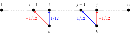
Figure 3. Canceling pairs of positive and negative covariances as $k$ passes through $1,\ldots,n-1$ in non-exceptional situations. The covariance is zero for all other values of $k$.

• If $i$ and $j$ are subsequent, i.e., $j=i+1,$ then the two locations in Figure 3 with positive contribution collide. If additionally $k=i$, we obtain $\mathrm{Cov}(\textbf{1}\{Z_{i}>Z_{j}\},\textbf{1}\{Z_{k}>Z_{k+1}\})=\mathrm{Cov}(\textbf{1}\{Z_{i}>Z_{i+1}\},\textbf{1}\{Z_{i}>Z_{i+1}\})=\mathrm{Var}(\textbf{1}\{Z_{i}>Z_{i+1}\})=1/4$.

• If $i=1,$ then the leftmost negative term in Figure 3 disappears.

• If $j=n,$ then the rightmost negative term in Figure 3 disappears.

As these situations are not mutually disjoint, we categorize the exceptional cases as follows:

• (E1): $j=i+1,$ but neither $i=1$ nor $j=n$.

• (E2): $i=1$ and $j=3,\ldots,n-1$.

• (E3): $j=n$ and $i=2,\ldots,n-2$.

• (E4): $i=1,$ $j=2$.

• (E5): $i=n-1$, $j=n$.

• (E6): $i=1$, $j=n$.

As an example, we display situation (E1) in Figure 4.

Figure 4. Display of covariances for the exceptional case (E1) when $i$ and $j=i+1$ are subsequent.

Looking at the contributions and frequencies of (E1), $\ldots,$ (E6), we obtain the exact result

$$\mathrm{Cov}(X_{\mathrm{inv}},X_{\mathrm{des}})=\underbrace{(n-3)\left(\frac{1}{4}-\frac{1}{6}\right)}_{(\mathrm{E}1)}+\underbrace{2(n-3)\frac{1}{12}}_{(\mathrm{E}2,~{}\mathrm{E}3)}+\underbrace{2\left(\frac{1}{4}-\frac{1}{12}\right)}_{(\mathrm{E}4,~{}\mathrm{E}5)}+\underbrace{\frac{1}{6}}_{(\mathrm{E}6)}=\frac{n-1}{4}.$$

The claim follows. ∎

8.2. Proof of Lemma 2.6b)

Recall that $Z_{1},\ldots,Z_{n}$ are i.i.d. $U(0,1)$. By Lemma 2.3, we have

$$\hat{X}_{\mathrm{inv}}=\sum_{j=1}^{n}(n-2j+1)Z_{j}+\frac{1}{2}\binom{n}{2},$$

which, together with the definition of $X_{\mathrm{des}}$, yields

$$\mathrm{Cov}(\hat{X}_{\mathrm{inv}},X_{\mathrm{des}}) =\mathrm{Cov}\left(\sum_{j=1}^{n}(n-2j+1)Z_{j},\sum_{k=1}^{n-1}\textbf{1}\{Z_{k}>Z_{k+1}\}\right)$$

$$=\Big{(}\sum_{j=2}^{n-1}+\sum_{j\in\{1,n\}}\Big{)}\sum_{k=1}^{n-1}(n-2j+1)\mathrm{Cov}(Z_{j},\textbf{1}\{Z_{k}>Z_{k+1}\})$$

$$=:T_{1}+T_{2}\,.$$

In view of the independence of $Z_{1},\ldots,Z_{n}$, we get

$$T_{1}=\sum_{j=2}^{n-1}(n-2j+1)\big{(}\mathrm{Cov}(Z_{j},\textbf{1}\{Z_{j}<Z_{j-1}\})+\mathrm{Cov}(Z_{j},\textbf{1}\{Z_{j}>Z_{j+1}\})\big{)}=0\,,$$

where for the last equality, we used

$$\mathrm{Cov}(Z_{j},\textbf{1}\{Z_{j}<Z_{j-1}\})+\mathrm{Cov}(Z_{j},\textbf{1}\{Z_{j}>Z_{j+1}\})$$

$$=\mathbb{E}(Z_{j}\textbf{1}\{Z_{j}<Z_{j-1}\})+\mathbb{E}(Z_{j}\textbf{1}\{Z_{j}>Z_{j+1}\})-\frac{1}{2}$$

$$=\mathbb{E}(Z_{j}\textbf{1}\{Z_{j}<Z_{j-1}\})+\mathbb{E}(Z_{j}\textbf{1}\{Z_{j}>Z_{j-1}\})-\frac{1}{2}$$

$$=\mathbb{E}(Z_{j})-\frac{1}{2}=0\,.$$

As $Z_{1}\textbf{1}\{Z_{1}<Z_{2}\}$ is a function in two uniform variables with joint density $f\negthickspace:\mathbb{R}^{2}\rightarrow\mathbb{R},(x,y)\mapsto\textbf{1}\{(x,y)\in[0,1]^{2}\}$, we can apply Fubini’s Theorem to obtain

$$\mathbb{E}(Z_{1}\textbf{1}\{Z_{1}<Z_{2}\}) =\int_{[0,1]^{2}}x\textbf{1}\{x<y\}\,\text{d}(x,y)$$

$$=\int_{0}^{1}x\left(\int_{0}^{1}\textbf{1}\{x<y\}\mathrm{d}y\right)\mathrm{d}x$$

$$=\int_{0}^{1}x(1-x)\,\mathrm{d}x=\frac{1}{6}.$$

Therefore, we get for $T_{2}$:

$$T_{2} =(n-1)\mathrm{Cov}(Z_{1},\textbf{1}\{Z_{1}>Z_{2}\})-(n-1)\mathrm{Cov}(Z_{n},\textbf{1}\{Z_{n-1}>Z_{n}\})$$

$$=(n-1)\big{(}\mathbb{E}(Z_{1}\textbf{1}\{Z_{1}>Z_{2}\})-\mathbb{E}(Z_{1}\textbf{1}\{Z_{1}<Z_{2}\})\big{)}$$

$$=(n-1)\big{(}1/2-2\mathbb{E}(Z_{1}\textbf{1}\{Z_{1}<Z_{2}\})\big{)}=\frac{n-1}{6}\,,$$

which shows that $\mathrm{Cov}(\hat{X}_{\mathrm{inv}},X_{\mathrm{des}})=\displaystyle{\frac{n-1}{6}}$. ∎

8.3. Proof of Lemma 5.3

We follow the instructive calculation of $\mathrm{Var}(X_{\mathrm{inv}})$ in the uniform case provided in [18, Section 3]. So, the main task is to calculate $\mathbb{E}(X_{\mathrm{inv}}^{2})$. For $X_{\mathrm{inv}}^{B},$ we recall (17a) and use the abbreviations

$$X_{\mathrm{inv}}^{B}=\underbrace{\sum_{i<j}\textbf{1}\{Z_{i}>Z_{j}\}}_{=:~{}X^{+}}+\underbrace{\sum_{i<j}\textbf{1}\{-Z_{i}>Z_{j}\}}_{=:~{}X^{-}}+\underbrace{\sum_{i=1}^{n}\textbf{1}\{Z_{i}<0\}}_{=:~{}X^{\circ}}=X^{+}+X^{-}+X^{\circ}.$$

This means we need to compute the terms

$$\mathbb{E}\bigl{(}(X_{\mathrm{inv}}^{B})^{2}\bigr{)} =\mathbb{E}((X^{+})^{2})+\mathbb{E}((X^{-})^{2})+2\mathbb{E}(X^{+}X^{-})$$

$$\qquad+\mathbb{E}((X^{\circ})^{2})+2\mathbb{E}(X^{+}X^{\circ})+2\mathbb{E}(X^{-}X^{\circ}).$$

The first term $\mathbb{E}((X^{+})^{2})$ is invariant under $p,$ since it only involves events $\{Z_{i}>Z_{j}\}$ for which $\mathbb{P}(Z_{i}>Z_{j})=1/2,$ even if the involved $Z_{i},Z_{j}$ are not uniformly distributed. Therefore, we can obtain $\mathbb{E}((X^{+})^{2})$ from [18, Section 3]:

$$\mathbb{E}((X^{+})^{2})=\frac{1}{2}\binom{n}{2}+\frac{1}{4}\binom{n}{2}\binom{n-2}{2}+\frac{5}{3}\binom{n}{3}.$$

Next, we turn to

$$\mathbb{E}((X^{-})^{2})=\sum_{i<j}\sum_{k<l}\mathbb{P}(-Z_{i}>Z_{j},-Z_{k}>Z_{l}).$$

For the $\binom{n}{2}\binom{n-2}{2}$ choices of pairwise distinct $i,j,k,l$, we have that $\mathbb{P}(-Z_{i}>Z_{j},-Z_{k}>Z_{l})=p^{2}$ by independence, and for the $\binom{n}{2}$ cases where $(i,j)=(k,l)$, we simply get $\mathbb{P}(-Z_{i}>Z_{j})=p$. The set of triples with two of the indices colliding need to be analyzed similarly as in the proof of Lemma 2.6a). Note that the cases $i=k$ and $j=l$ each contain two contributions. E.g., in the case of $i=l,$ we calculate by case distinction according to the signs:

$$\mathbb{P}(-Z_{i}>Z_{j},-Z_{k}>Z_{i}) =\mathbb{P}(-Z_{i}>Z_{j},-Z_{k}>Z_{i},Z_{i}>0)$$

$$\qquad+\mathbb{P}(-Z_{i}>Z_{j},-Z_{k}>Z_{i},Z_{i}<0)$$

$$=\mathbb{P}(-Z_{i}>Z_{j},-Z_{k}>Z_{i},Z_{i}>0,Z_{j}<0,Z_{k}<0)$$

$$\qquad+\mathbb{P}(Z_{i}<0,Z_{j}<0,Z_{k}<0)$$

$$\qquad+\mathbb{P}(Z_{i}<0,Z_{j}>0,Z_{k}<0,-Z_{i}>Z_{j})$$

$$\qquad+\mathbb{P}(Z_{i}<0,Z_{j}<0,Z_{k}>0,-Z_{k}>Z_{i})$$

$$\qquad+\mathbb{P}(Z_{i}<0,Z_{j}>0,Z_{k}>0,-Z_{i}>Z_{j},-Z_{k}>Z_{i})$$

$$=\frac{1}{3}p^{2}q+p^{3}+\frac{1}{2}p^{2}q+\frac{1}{2}p^{2}q+\frac{1}{3}pq^{2}$$

$$=\frac{1}{3}p(2p+1).$$

It turns out that all six constellations of triplets give this contribution. So, overall,

$$\mathbb{E}\bigl{(}(X^{-})^{2}\bigr{)}=\binom{n}{2}p+\binom{n}{2}\binom{n-2}{2}p^{2}+\binom{n}{3}2p(2p+1).$$

For $\mathbb{E}(X^{+}X^{-}),$ the disjoint quadruplets give a contribution of $p/2$ each. For the colliding pairs, we need to compute

$$\mathbb{P}(Z_{i}>Z_{j},-Z_{i}>Z_{j})$$

$$=~{} \underbrace{\mathbb{P}(Z_{i}>Z_{j},-Z_{i}>Z_{j},Z_{i}>0,Z_{j}>0)}_{=~{}0}+\underbrace{\mathbb{P}(Z_{i}>Z_{j},-Z_{i}>Z_{j},Z_{i}<0,Z_{j}>0)}_{=~{}0}$$

$$\quad+\mathbb{P}(Z_{i}>Z_{j},-Z_{i}>Z_{j},Z_{i}<0,Z_{j}<0)+\mathbb{P}(Z_{i}>Z_{j},-Z_{i}>Z_{j},Z_{i}>0,Z_{j}<0)$$

$$=~{} \mathbb{P}(Z_{i}<0,Z_{j}<0,Z_{i}>Z_{j})+\mathbb{P}(Z_{i}>0,Z_{j}<0,-Z_{i}>Z_{j})=\frac{p^{2}}{2}+p^{2}q.$$

For the triplets, we repeat the procedure above. For the cases $j=k$ and $j=l$, we get

$$\mathbb{P}(Z_{i}>Z_{j},-Z_{j}>Z_{k})=-\frac{1}{6}p(2p-5).$$

For the cases $i=l$ and $i=k$, we derive

$$\mathbb{P}(Z_{i}>Z_{j},-Z_{i}>Z_{l}) =\mathbb{P}(Z_{i}>Z_{j},-Z_{i}>Z_{l},Z_{i}>0,Z_{l}<0)$$

$$\qquad+\mathbb{P}(Z_{i}>Z_{j},-Z_{i}>Z_{l},Z_{i}<0,Z_{j}<0)$$

$$=\mathbb{P}(Z_{i}>0,Z_{j}<0,Z_{l}<0,-Z_{i}>Z_{l})$$

$$\qquad+\mathbb{P}(Z_{i}>0,Z_{j}>0,Z_{l}<0,Z_{j}<Z_{i}<-Z_{l})$$

$$\qquad+\mathbb{P}(Z_{i}<0,Z_{j}<0,Z_{l}<0,Z_{i}>Z_{j})$$

$$\qquad+\mathbb{P}(Z_{i}<0,Z_{j}<0,Z_{l}>0,Z_{j}<Z_{i}<-Z_{l})$$

$$=\frac{1}{2}p^{2}q+\frac{1}{6}pq^{2}+\frac{1}{2}p^{3}+\frac{1}{6}p^{2}q$$

$$=\frac{1}{6}p(2p+1),$$

and overall we obtain

$$\mathbb{E}(X^{+}X^{-}) =\binom{n}{2}\left(\frac{p^{2}}{2}+p^{2}q\right)+\binom{n}{2}\binom{n-2}{2}\frac{p}{2}+3\binom{n}{3}\underbrace{\biggl{(}\frac{1}{6}p(2p+1)-\frac{1}{6}p(2p-5)\biggr{)}}_{=~{}p}$$

$$=\binom{n}{2}\left(\frac{p^{2}}{2}+p^{2}q\right)+\binom{n}{2}\binom{n-2}{2}\frac{p}{2}+3\binom{n}{3}p.$$

The remaining three terms are easily calculated as

$$\mathbb{E}(X^{+}X^{\circ}) =\sum_{i<j}\sum_{k=1}^{n}\mathbb{P}(Z_{i}>Z_{j},Z_{k}<0)$$

$$=3\binom{n}{3}\frac{p}{2}+\sum_{i<j}\mathbb{P}(Z_{i}>Z_{j},Z_{i}<0)+\sum_{i<j}\mathbb{P}(Z_{i}>Z_{j},Z_{j}<0)$$

$$=3\binom{n}{3}\frac{p}{2}+\binom{n}{2}(p^{2}+pq)=3\binom{n}{3}\frac{p}{2}+\binom{n}{2}p,$$

$$\mathbb{E}(X^{-}X^{\circ}) =\sum_{i<j}\sum_{k=1}^{n}\mathbb{P}(-Z_{i}>Z_{j},Z_{k}<0)$$

$$=3\binom{n}{3}p^{2}+2\binom{n}{2}(p^{2}+p^{2}q)=3\binom{n}{3}p^{2}+2\binom{n}{2}(2p^{2}-p^{3}),$$

$$\mathbb{E}((X^{\circ})^{2}) =\sum_{i,j=1}^{n}\mathbb{P}(Z_{i}<0,Z_{j}<0)=2\binom{n}{2}p^{2}+np.$$

Summing all of these terms and subtracting the square of the mean gives the claim for $B_{n}$. On $D_{n},$ we ignore the parts involving $X^{\circ}$ and get the desired result. ∎

8.4. Proof of Lemma 5.4

We first prove the claim on the even-signed permutation groups $D_{n}$, since the calculation will be the same for $B_{n}$. We proceed as in Lemma 2.3, starting from

$$\hat{X}_{\mathrm{inv}}=\sum_{k=1}^{n}\mathbb{E}(X_{\mathrm{inv}}\mid Z_{k})-(n-1)\mathbb{E}(X_{\mathrm{inv}}),$$

except here, $X_{\mathrm{inv}}$ is defined by (17b), and we have $Z_{k}\sim\mathrm{GR}(p)$. According to (17b), we have

$$\mathbb{E}(X_{\mathrm{inv}}\mid Z_{k}) =\sum_{i<j}\mathbb{E}\bigl{(}\textbf{1}\{Z_{i}>Z_{j}\}+\textbf{1}\{-Z_{i}>Z_{j}\}\mid Z_{k}\bigr{)}$$

(21) $$=\sum_{i<j}\big{(}\mathbb{P}(Z_{i}>Z_{j}\mid Z_{k})+\mathbb{P}(-Z_{i}>Z_{j}\mid Z_{k})\big{)}.$$

Write $f(Z_{i},Z_{j}):=\mathbf{1}\{Z_{i}>Z_{j}\}+\mathbf{1}\{-Z_{i}>Z_{j}\}$ for $i<j$ and set $U_{k}=|Z_{k}|$. A straightforward case distinction gives

$Z_{i},Z_{j}>0$: $f(Z_{i},Z_{j})=\textbf{1}\{U_{i}>U_{j}\},$

$Z_{i}>0,Z_{j}<0$: $f(Z_{i},Z_{j})=\textbf{1}\{U_{i}>U_{j}\},$

$Z_{i}<0,Z_{j}>0$: $f(Z_{i},Z_{j})=\textbf{1}\{U_{i}<U_{j}\}+1,$

$Z_{i},Z_{j}<0$: $f(Z_{i},Z_{j})=\textbf{1}\{U_{i}<U_{j}\}+1$. For symmetry reasons, $f(Z_{i},Z_{j})$ depends only on the sign of $Z_{i}$ but not on the sign of $Z_{j}$. To compute (21), we only need to consider the $n-k$ tuples $(k,j)$ and the $k-1$ tuples $(i,k)$, as the other tuples are independent of $Z_{k}$ and produce constants which do not contribute to the variance.

Recall that for $k<j$, we have $\mathbb{P}(U_{k}>U_{j}\mid U_{k})=U_{k}$ and $\mathbb{P}(U_{k}<U_{j}\mid U_{k})=1-U_{k}$. Therefore, we can write

$$\mathbb{E}(X_{\mathrm{inv}}\mid Z_{k})=\sum_{i=1}^{k-1}\mathbb{E}\bigl{(}f(Z_{i},Z_{k})\mid Z_{k}\bigr{)}+\sum_{j=k+1}^{n}\mathbb{E}\bigl{(}f(Z_{k},Z_{j})\mid Z_{k}\bigr{)},$$

where

$$\mathbb{E}\bigl{(}f(Z_{i},Z_{k})\mid Z_{k}\bigr{)} =\mathbb{P}(Z_{i}>0)(1-U_{k})+\mathbb{P}(Z_{i}<0)(1+U_{k})$$

$$=q(1-U_{k})+p(1+U_{k})=2pU_{k}-U_{k}+1$$

and

$$\mathbb{E}\bigl{(}f(Z_{k},Z_{j})\mid Z_{k}\bigr{)} =\textbf{1}\{Z_{k}>0\}U_{k}+\textbf{1}\{Z_{k}<0\}(1+1-U_{k})$$

$$=\textbf{1}\{Z_{k}>0\}U_{k}+\textbf{1}\{Z_{k}<0\}(2-U_{k}).$$

Overall, we obtain

$$\mathbb{E}(X_{\mathrm{inv}}\mid Z_{k}) =(k-1)(2pU_{k}-U_{k}+1)$$

$$\quad+(n-k)\bigl{(}\textbf{1}\{Z_{k}>0\}U_{k}+\textbf{1}\{Z_{k}<0\}(2-U_{k})\bigr{)}+\text{const}.$$

To use the standard formula $\mathrm{Var}(X)=\mathbb{E}(X^{2})-\mathbb{E}(X)^{2},$ where $X$ is not affected by constant summands, we now compute

$$\mathbb{E}(\mathbb{E}(X_{\mathrm{inv}}\mid Z_{k})^{2})$$

(22a) $$=~{} (k-1)^{2}\mathbb{E}\left((2pU_{k}-U_{k}+1)^{2}\right)$$

(22b) $$+~{} (n-k)^{2}\mathbb{E}\left(\bigl{(}\textbf{1}\{Z_{k}>0\}U_{k}+\textbf{1}\{Z_{k}<0\}(2-U_{k})\bigr{)}^{2}\right)$$

(22c) $$+~{} 2(k-1)(n-k)\mathbb{E}\left((2pU_{k}-U_{k}+1)\bigl{(}\textbf{1}\{Z_{k}>0\}U_{k}\right.$$

$$\hskip 167.87108pt+\left.\textbf{1}\{Z_{k}<0\}(2-U_{k})\bigr{)}\right).$$

The random variables $\textbf{1}\{Z_{k}>0\}$ and $U_{k}$ are independent by construction and therefore,

$$\eqref{24a} =(k-1)^{2}\mathbb{E}\left(4p^{2}U_{k}^{2}-4pU_{k}^{2}+4pU_{k}+U_{k}^{2}-2U_{k}+1\right)$$

$$=(k-1)^{2}\left(\frac{4}{3}p^{2}-\frac{4}{3}p+2p+\frac{1}{3}\right)=(k-1)^{2}\left(\frac{4}{3}p^{2}+\frac{2}{3}p+\frac{1}{3}\right),$$

$$\eqref{24b} =(n-k)^{2}\left(q\mathbb{E}(U_{k})^{2}+p\mathbb{E}\bigl{(}(2-U_{k})^{2}\bigr{)}\right)$$

$$=(n-k)^{2}\left(\frac{q}{3}+\frac{7}{3}p\right)=(n-k)^{2}\left(2p+\frac{1}{3}\right),$$

$$\eqref{24c} =2(k-1)(n-k)\Bigl{(}(1-p)\mathbb{E}(2pU_{k}^{2}-U_{k}^{2}+U_{k})$$

$$\hskip 85.35826pt+p\mathbb{E}\bigl{(}(2pU_{k}-U_{k}+1)(2-U_{k})\bigr{)}\Bigr{)}$$

$$=2(k-1)(n-k)\left((1-p)\left(\frac{2}{3}p+\frac{1}{6}\right)+p\left(\frac{4}{3}p+\frac{5}{6}\right)\right)$$

$$=2(k-1)(n-k)\left(\frac{2}{3}p^{2}+\frac{4p}{3}+\frac{1}{6}\right).$$

In total, we have

$$\mathbb{E}(\mathbb{E}(X_{\mathrm{inv}}\mid Z_{k})^{2}) =(k-1)^{2}\left(\frac{4}{3}p^{2}+\frac{2}{3}p+\frac{1}{3}\right)+(n-k)^{2}\left(2p+\frac{1}{3}\right)$$

$$+2(k-1)(n-k)\left(\frac{2}{3}p^{2}+\frac{4}{3}p+\frac{1}{6}\right).$$

We subtract the square of

$$\mathbb{E}(\mathbb{E}(X_{\mathrm{inv}}\mid Z_{k})) =(k-1)\left(p+\frac{1}{2}\right)+(n-k)\left(\frac{1}{2}-\frac{p}{2}+\frac{3}{2}p\right)$$

$$=\left(p+\frac{1}{2}\right)(n-1).$$

The variance of $\hat{X}_{\mathrm{inv}}$ on $D_{n}$ is

$$\mathrm{Var}(\hat{X}_{\mathrm{inv}}) =\sum_{k=1}^{n}\Big{(}\mathbb{E}(\mathbb{E}(X_{\mathrm{inv}}\mid Z_{k})^{2})-\mathbb{E}(\mathbb{E}(X_{\mathrm{inv}}\mid Z_{k}))^{2}\Big{)}$$

$$=\sum_{k=1}^{n}\mathbb{E}(\mathbb{E}(X_{\mathrm{inv}}\mid Z_{k})^{2})-n(n-1)^{2}\left(p+\frac{1}{2}\right)^{2},$$

so, to conclude the proof, we compute

$$\sum_{k=1}^{n}\mathbb{E}(\mathbb{E}(X_{\mathrm{inv}}\mid Z_{k})^{2}) =\left(\frac{4}{3}p^{2}+\frac{2}{3}p+\frac{1}{3}\right)\sum_{k=1}^{n}(k-1)^{2}+\left(2p+\frac{1}{3}\right)\sum_{k=1}^{n}(n-k)^{2}$$

$$\qquad+\left(\frac{4}{3}p^{2}+\frac{8p}{3}+\frac{1}{3}\right)\sum_{k=1}^{n}(k-1)(n-k)$$

$$=\left(\frac{4}{3}p^{2}+\frac{2}{3}p+\frac{1}{3}\right)\cdot\frac{1}{6}n(n-1)(2n-1)$$

$$\qquad+\left(2p+\frac{1}{3}\right)\cdot\frac{1}{6}n(n-1)(2n-1)$$

$$\qquad+\left(\frac{4}{3}p^{2}+\frac{8p}{3}+\frac{1}{3}\right)\cdot\frac{1}{6}n(n-1)(n-2)$$

$$=n^{3}\left(\frac{2}{3}p^{2}+\frac{4}{3}p+\frac{5}{18}\right)-n^{2}\left(\frac{4}{3}p^{2}-\frac{8}{3}p-\frac{1}{2}\right)$$

$$\qquad+n\left(\frac{2}{3}p^{2}+\frac{4}{3}p+\frac{2}{9}\right).$$

Subtracting $n(n-1)^{2}\left(p+\frac{1}{2}\right)^{2}$ gives exactly the desired leading term computed in Lemma 5.3. On the groups $B_{n},$ we achieve the same result since the extra parts in $\mathrm{Var}(\hat{X}_{\mathrm{inv}})$ yielded by $\sum_{i=1}^{n}\textbf{1}\{Z_{i}<0\}$ are not significant. Recall that

$$X_{\mathrm{inv}}^{B}=X_{\mathrm{inv}}^{D}+\sum_{i=1}^{n}\textbf{1}\{Z_{i}<0\},$$

and therefore,

$$\mathrm{Var}\left(\mathbb{E}(X_{\mathrm{inv}}^{B}\mid Z_{k})\right) =\mathrm{Var}\left(\mathbb{E}(X_{\mathrm{inv}}^{D}\mid Z_{k})+\sum_{j=1}^{n}\mathbb{E}(\textbf{1}\{Z_{j}<0\}\mid Z_{k})\right)$$

$$=\mathrm{Var}\left(\mathbb{E}(X_{\mathrm{inv}}^{D}\mid Z_{k})+\mathbb{E}(\textbf{1}\{Z_{k}<0\}\mid Z_{k})+\text{const}\right)$$

$$=\mathrm{Var}\left(\mathbb{E}(X_{\mathrm{inv}}^{D}\mid Z_{k})+\textbf{1}\{Z_{k}<0\}+\text{const}\right)$$

$$=\mathrm{Var}\hskip 1.99168pt\Bigl{(}(n-k)\textbf{1}\{Z_{k}>0\}U_{k}+(n-k)\textbf{1}\{Z_{k}<0\}(2-U_{k})$$

$$\hskip 45.52458pt+(k-1)(2pU_{k}-U_{k}+1)+\textbf{1}\{Z_{k}<0\}+\text{const}\Bigr{)}.$$

Using the standard formula again, we have

$$\mathbb{E}\left(\mathbb{E}(X_{\mathrm{inv}}^{B}\mid Z_{k})^{2}\right) =\mathbb{E}\left(\mathbb{E}(X_{\mathrm{inv}}^{D}\mid Z_{k})^{2}\right)+\mathbb{E}\left(\textbf{1}\{Z_{k}<0\}\right)$$

$$\qquad+2\mathbb{E}\left((n-k)(2-U_{k})\textbf{1}\{Z_{k}<0\}\right)$$

$$\qquad+2\mathbb{E}\bigl{(}(k-1)(2pU_{k}-U_{k}+1)\textbf{1}\{Z_{k}<0\}\bigr{)}$$

$$=\mathbb{E}\left(\mathbb{E}(X_{\mathrm{inv}}^{D}\mid Z_{k})^{2}\right)+p+3p(n-k)+(k-1)(2p+1)p,$$

$$\mathbb{E}\left(\mathbb{E}(X_{\mathrm{inv}}^{B}\mid Z_{k})\right)^{2} =\mathbb{E}\left(\mathbb{E}(X_{\mathrm{inv}}^{D}\mid Z_{k})\right)^{2}+p^{2}+2\mathbb{E}(\textbf{1}\{Z_{k}<0\})\mathbb{E}\left(\mathbb{E}(X_{\mathrm{inv}}^{D}\mid Z_{k})\right)$$

$$=\left(p+\frac{1}{2}\right)^{2}(n-1)^{2}+p^{2}+2p(n-1)\left(p+\frac{1}{2}\right).$$

We conclude that

$$\mathrm{Var}(\hat{X}_{\mathrm{inv}}^{B}) =\mathrm{Var}(\hat{X}_{\mathrm{inv}}^{D})+n(p-p^{2})-p(2p+1)\frac{n(n-1)}{2}$$

$$=\mathrm{Var}(\hat{X}_{\mathrm{inv}}^{D})+O(n^{2}).$$

The desired claim follows from Theorem 2.2. ∎

8.5. Proof of Lemma 5.6a)

For the groups $B_{n}$ and $D_{n},$ the calculation follows the same approach as on $S_{n}$. Recall that now, $Z_{1},\ldots,Z_{n}\sim\mathrm{GR}(p).$ On $D_{n},$ we have by (16b), (17b) that

(23a) $$\mathrm{Cov}(X_{\mathrm{inv}}^{D},X_{\mathrm{des}}^{D}) =\sum_{i<j}\sum_{k=1}^{n-1}\mathrm{Cov}\left(\textbf{1}\{Z_{i}>Z_{j}\},\textbf{1}\{Z_{k}>Z_{k+1}\}\right)$$

(23b) $$+\sum_{i<j}\sum_{k=1}^{n-1}\mathrm{Cov}\left(\textbf{1}\{-Z_{i}>Z_{j}\},\textbf{1}\{Z_{k}>Z_{k+1}\}\right)$$

(23c) $$+\sum_{i<j}\mathrm{Cov}(\textbf{1}\{Z_{i}>Z_{j}\}+\textbf{1}\{-Z_{i}>Z_{j}\},\textbf{1}\{-Z_{2}>Z_{1}\}).$$

The contribution of (23a) is $(n-1)/4,$ in analogy with Lemma 2.6a). In (23b), we first demonstrate the cancellation in the non-exceptional case when $\{i-1,i,j-1,j\}$ form a set of distinct numbers. In that case, we have

$$\mathrm{Cov}(\textbf{1}\{-Z_{i}>Z_{j}\},\textbf{1}\{Z_{i}>Z_{i+1}\})+\mathrm{Cov}(\textbf{1}\{-Z_{i}>Z_{j}\},\textbf{1}\{Z_{i-1}>Z_{i}\})$$

$$=~{} \mathbb{E}(\textbf{1}\{-Z_{i}>Z_{j}\}\textbf{1}\{Z_{i}>Z_{i+1}\})+\mathbb{E}(\textbf{1}\{-Z_{i}>Z_{j}\}\textbf{1}\{Z_{i-1}>Z_{i}\})-2(p/2)$$

$$=~{} \mathbb{E}(\textbf{1}\{-Z_{i}>Z_{j}\}\textbf{1}\{Z_{i}>Z_{i+1}\})+\mathbb{E}(\textbf{1}\{-Z_{i}>Z_{j}\}\textbf{1}\{Z_{i+1}>Z_{i}\})-p$$

$$=~{} \mathbb{E}(\textbf{1}\{-Z_{i}>Z_{j}\})-p=0,$$

and likewise,

$$\mathrm{Cov}(\textbf{1}\{-Z_{i}>Z_{j}\},\textbf{1}\{Z_{j}>Z_{j+1}\})+\mathrm{Cov}(\textbf{1}\{-Z_{i}>Z_{j}\},\textbf{1}\{Z_{j-1}>Z_{j}\})=0.$$

However, this cancellation occurs not only in the non-exceptional cases, but also in the aggregation of the exceptional cases (E1) – (E6) from the proof of Lemma 2.6a), except for the covariances resulting from the clash of $j=i+1$ and $k=i$. To be precise, (E2) and (E3) cancel mutually. (E4) and (E5) give two clashes and a canceling pair. (E6) consists of another canceling pair. All of this can be checked from the computation of $\mathbb{E}(X^{+}X^{-})$ in the proof of Lemma 5.3. From there, we also obtain $\forall i=1,\ldots,n-1$:

$$\mathrm{Cov}(\textbf{1}\{-Z_{i}>Z_{i+1}\},\textbf{1}\{Z_{i}>Z_{i+1}\})=\frac{p^{2}}{2}+p^{2}q-\frac{p}{2},$$

which interestingly vanishes in the unbiased case. Overall,

$$\eqref{21b}=(n-1)\left(\frac{p^{2}}{2}+p^{2}q-\frac{p}{2}\right).$$

Finally, consider (23c). Obviously, this double-indexed sum involves exactly the pairs $(i,j)$ with $i=1$ or $i=2$. We get

$$\eqref{21c} =\sum_{j=3}^{n}\mathrm{Cov}(\textbf{1}\{Z_{1}>Z_{j}\}+\textbf{1}\{-Z_{1}>Z_{j}\},\textbf{1}\{-Z_{2}>Z_{1}\})$$

$$+\sum_{j=3}^{n}\Big{[}\mathrm{Cov}(\textbf{1}\{Z_{2}>Z_{j}\}+\textbf{1}\{-Z_{2}>Z_{j}\},\textbf{1}\{-Z_{2}>Z_{1}\})$$

$$+\underbrace{\mathrm{Cov}(\textbf{1}\{-Z_{1}>Z_{2}\},\textbf{1}\{-Z_{2}>Z_{1}\})}_{=\hskip 1.99168ptp^{2}}+\underbrace{\mathrm{Cov}(\textbf{1}\{Z_{1}>Z_{2}\},\textbf{1}\{-Z_{2}>Z_{1}\})}_{=\hskip 1.99168pt0}\Big{]}$$

$$=\underbrace{\sum_{j=3}^{n}\Big{[}\mathrm{Cov}(\textbf{1}\{Z_{1}>Z_{j}\},\textbf{1}\{-Z_{2}>Z_{1}\})+\mathrm{Cov}(\textbf{1}\{-Z_{1}>Z_{j}\},\textbf{1}\{-Z_{2}>Z_{1}\})\Big{]}}_{=\hskip 1.99168pt0}$$

$$+\underbrace{\sum_{j=3}^{n}\Big{[}\mathrm{Cov}(\textbf{1}\{Z_{2}>Z_{j}\},\textbf{1}\{-Z_{2}>Z_{1}\})+\mathrm{Cov}(\textbf{1}\{-Z_{2}>Z_{j}\},\textbf{1}\{-Z_{2}>Z_{1}\})\Big{]}}_{=\hskip 1.99168pt0}+\hskip 1.99168ptp^{2}.$$

Therefore, we obtain the overall result on $D_{n}$, which is

$$\mathrm{Cov}(X_{\mathrm{inv}}^{D},X_{\mathrm{des}}^{D})=(n-1)\left(\frac{p^{2}}{2}+p^{2}q-\frac{p}{2}+\frac{1}{4}\right)+p^{2}.$$

Next, we show that this result is obtained on $B_{n}$ as well. By (17a) and (16a), we have

$$\mathrm{Cov}(X_{\mathrm{inv}}^{B},X_{\mathrm{des}}^{B}) =\eqref{21a}+\eqref{21b}$$

(24a) $$+\sum_{i=1}^{n}\sum_{k=1}^{n-1}\mathrm{Cov}(\textbf{1}\{Z_{i}<0\},\textbf{1}\{Z_{k}>Z_{k+1}\})$$

(24b) $$+\sum_{i<j}\mathrm{Cov}(\textbf{1}\{Z_{i}>Z_{j}\}+\textbf{1}\{-Z_{i}>Z_{j}\},\textbf{1}\{Z_{1}<0\})$$

(24c) $$+\sum_{i=1}^{n}\mathrm{Cov}(\textbf{1}\{Z_{i}<0\},\textbf{1}\{Z_{1}<0\})\,.$$

We now see that (24a) and (24b) vanish. In (24a), the inner sum only involves $k=i-1$ and $k=i,$ therefore,

$$\eqref{22a} =\sum_{i=1}^{n}\Big{[}\mathrm{Cov}(\textbf{1}\{Z_{i}<0\},\textbf{1}\{Z_{i-1}>Z_{i}\})+\mathrm{Cov}(\textbf{1}\{Z_{i}<0\},\textbf{1}\{Z_{i}>Z_{i+1}\})\Big{]}$$

$$=\sum_{i=1}^{n}\Big{[}\mathrm{Cov}(\textbf{1}\{Z_{i}<0\},\textbf{1}\{Z_{i-1}>Z_{i}\})+\mathrm{Cov}(\textbf{1}\{Z_{i}<0\},\textbf{1}\{Z_{i}>Z_{i-1}\})\Big{]}$$

$$=\mathbb{E}(\textbf{1}\{Z_{1}<0\})-2p/2=0.$$

This cancellation even applies to the border terms $i=1$ and $i=n$. We also get

$$\eqref{22b} =\sum_{j=2}^{n}\Big{[}\mathrm{Cov}(\textbf{1}\{Z_{1}>Z_{j}\},\textbf{1}\{Z_{1}<0\})+\mathrm{Cov}(\textbf{1}\{-Z_{1}>Z_{j}\},\textbf{1}\{Z_{1}<0\})\Big{]}$$

$$=\underbrace{\sum_{j=2}^{n}\Big{[}\mathbb{P}(Z_{1}<0,Z_{1}>Z_{j})-p/2\Big{]}}_{=\hskip 1.99168pt-pq/2}+\underbrace{\sum_{j=2}^{n}\Big{[}\mathbb{P}(Z_{1}<0,-Z_{1}>Z_{j})-p^{2}\Big{]}}_{=\hskip 1.99168ptpq/2}=0.$$

Finally,

$$\eqref{22c}=\sum_{i=1}^{n}\mathrm{Cov}(\textbf{1}\{Z_{i}<0\},\textbf{1}\{Z_{1}<0\})=\mathrm{Var}(\textbf{1}\{Z_{1}<0\})=p-p^{2},$$

giving the overall result

$$\mathrm{Cov}(X_{\mathrm{inv}}^{B},X_{\mathrm{des}}^{B})=(n-1)\left(\frac{p^{2}}{2}+p^{2}q-\frac{p}{2}+\frac{1}{4}\right)+(p-p^{2}),$$

so again, $\mathrm{Corr}(X_{\mathrm{inv}}^{B},X_{\mathrm{des}}^{B})$ vanishes in the limit. ∎

8.6. Proof of Lemma 5.6b)

For the groups $B_{n}$ and $D_{n}$, with $Z_{k}\sim\mathrm{GR}(p)$ and the modifications (16a), (16b), the calculation is more extensive but its procedure is the same as in the proof of Lemma 2.6b). On $D_{n}$, we first have

(25a) $$\mathrm{Cov}(\hat{X}_{\mathrm{inv}}^{D},X_{\mathrm{des}}^{D})=\sum_{j=1}^{n}\sum_{k=1}^{n-1} (n-j)\mathrm{Cov}(U_{j}\textbf{1}\{Z_{j}>0\},\textbf{1}\{Z_{k}>Z_{k+1}\})$$

(25b) $$+~{} (n-j)\mathrm{Cov}((2-U_{j})\textbf{1}\{Z_{j}<0\},\textbf{1}\{Z_{k}>Z_{k+1}\})$$

(25c) $$+~{} (j-1)\mathrm{Cov}(2pU_{j}-U_{j}+1,\textbf{1}\{Z_{k}>Z_{k+1}\}).$$

(25d) $$+\sum_{j=1}^{n} (n-j)\mathrm{Cov}(U_{j}\textbf{1}\{Z_{j}>0\},\textbf{1}\{-Z_{2}>Z_{1}\})$$

(25e) $$+~{} (n-j)\mathrm{Cov}((2-U_{j})\textbf{1}\{Z_{j}<0\},\textbf{1}\{-Z_{2}>Z_{1}\})$$

(25f) $$+~{} (j-1)\mathrm{Cov}(2pU_{j}-U_{j}+1,\textbf{1}\{-Z_{2}>Z_{1}\}).$$

In the first three rows (25a) – (25c), there is cancellation if $j\notin\{1,n\}$ due to previously used arguments. Only $j=1$ is relevant in (25a), (25b) and only $j=n$ is relevant in (25c). We have $\mathbb{E}(U_{j}\textbf{1}\{Z_{j}>0\})\mathbb{E}(\textbf{1}\{Z_{j}>Z_{j+1}\})=q/4$, and the joint density of $Z_{j}$ and $Z_{j+1}$ is

$$f_{p}(x,y):=f_{p}(x)f_{p}(y)=\begin{cases}p^{2},&x,y<0\\ pq,&x>0,y<0\\ pq,&x<0,y>0\\ q^{2},&x,y>0\end{cases}.$$

By Fubini’s Theorem, we obtain

$$\mathbb{E}(U_{1} \textbf{1}\{Z_{1}>0\}\textbf{1}\{Z_{1}>Z_{2}\})=\int_{[-1,1]^{2}}|x|\textbf{1}\{x>0\}\textbf{1}\{x>y\}f_{p}(x,y)\text{d}(x,y)$$

$$=\int_{[0,1]^{2}}q^{2}x\textbf{1}\{x>y\}\text{d}(x,y)+\int_{[0,1]\times[-1,0]}pqx\textbf{1}\{x>y\}\text{d}(x,y)$$

$$=q^{2}\int_{0}^{1}x^{2}dx+pq\int_{0}^{1}x\mathrm{d}x=\frac{q^{2}}{3}+\frac{pq}{2},$$

and likewise,

$$\mathbb{E}\bigl{(}(2-U_{1})\textbf{1}\{Z_{1}<0\}\textbf{1}\{Z_{1}>Z_{2}\}\bigr{)} =\int_{-1}^{0}\int_{-1}^{1}(2-|x|)\textbf{1}\{x>y\}f_{p}(x,y)\text{d}(x,y)$$

$$=p^{2}\int_{-1}^{0}(2+x)(1+x)\mathrm{d}x=\frac{5}{6}p^{2},$$

$$\mathbb{E}\bigl{(}(2p-1)U_{n}\textbf{1}\{Z_{n-1}>Z_{n}\}\bigr{)} =(2p-1)\int_{[-1,1]^{2}}|x|\textbf{1}\{x<y\}f_{p}(x,y)\text{d}(x,y)$$

$$=(2p-1)\left(\frac{p^{2}}{3}+\frac{q^{2}}{6}+\frac{pq}{2}\right)=(2p-1)\frac{p+1}{6}.$$

Therefore,

$$\eqref{23a}+\eqref{23b}+\eqref{23c}=(n-1)\left(-\frac{p^{3}}{3}+\frac{5p^{2}}{3}-\frac{4p}{3}+\frac{1}{6}\right)$$

has linear order. The remaining three rows (25d) – (25f) also have no more than linear order, since the summands are nonzero only for $j=1$ or $j=2$. ∎

References

- [1] Arslan, İ., Işlak, Ü., and Pehlivan, C. On unfair permutations. Statistics & Probability Letters 141 (2018), 31–40.
- [2] Bender, E. A. Central and local limit theorems applied to asymptotic enumeration. Journal of Combinatorial Theory, Series A 15, 1 (1973), 91–111.
- [3] Björner, A., and Brenti, F. Combinatorics of Coxeter groups, vol. 231. Springer Science & Business Media, 2006.
- [4] Brück, B., and Röttger, F. A central limit theorem for the two-sided descent statistic on Coxeter groups. Electronic Journal of Combinatorics 29, 1 (2022), P1.1.
- [5] Chang, J., Chen, X., and Wu, M. Central limit theorems for high dimensional dependent data. arXiv preprint arXiv:2104.12929 (2021).
- [6] Chatterjee, S., and Diaconis, P. A central limit theorem for a new statistic on permutations. Indian Journal of Pure and Applied Mathematics 48, 4 (2017), 561–573.
- [7] Chernozhukov, V., Chetverikov, D., and Kato, K. Gaussian approximations and multiplier bootstrap for maxima of sums of high-dimensional random vectors. The Annals of Statistics 41, 6 (2013), 2786–2819.
- [8] Chernozhukov, V., Chetverikov, D., and Kato, K. Central limit theorems and bootstrap in high dimensions. The Annals of Probability 45, 4 (2017), 2309–2352.
- [9] Chernozhukov, V., Chetverikov, D., and Koike, Y. Nearly optimal central limit theorem and bootstrap approximations in high dimensions. The Annals of Applied Probability 33, 3 (2023), 2374–2425.
- [10] Conger, M. A Refinement of the Eulerian Numbers, and the Joint Distribution of and Des() in . arXiv preprint math/0508112 (2005).
- [11] Conger, M., and Viswanath, D. Normal approximations for descents and inversions of permutations of multisets. Journal of Theoretical Probability 20, 2 (2007), 309–325.
- [12] Das, D., and Lahiri, S. Central limit theorem in high dimensions: The optimal bound on dimension growth rate. Transactions of the American Mathematical Society 374, 10 (2021), 6991–7009.
- [13] Dörr, P., and Kahle, T. Extreme values of permutation statistics. arXiv preprint arXiv:2205.01426 (2022).
- [14] Fang, X., and Koike, Y. High-dimensional central limit theorems by Stein’s method. The Annals of Applied Probability 31, 4 (2021), 1660–1686.
- [15] Fang, X., and Röllin, A. Rates of convergence for multivariate normal approximation with applications to dense graphs and doubly indexed permutation statistics. Bernoulli 21, 4 (2015), 2157–2189.
- [16] Fulman, J. Stein’s method and non-reversible markov chains. Lecture Notes-Monograph Series (2004), 69–77.
- [17] Harper, L. H. Stirling behavior is asymptotically normal. Ann. Math. Statist. 38 (1967), 410–414.
- [18] Kahle, T., and Stump, C. Counting inversions and descents of random elements in finite Coxeter groups. Mathematics of Computation 89, 321 (2020), 437–464.
- [19] Koike, Y. Notes on the dimension dependence in high-dimensional central limit theorems for hyperrectangles. Japanese Journal of Statistics and Data Science 4, 1 (2021), 257–297.
- [20] Leadbetter, M. R., Lindgren, G., and Rootzén, H. Extremes and related properties of random sequences and processes. Springer Science & Business Media, 1983.
- [21] Meier, K., and Stump, C. Central limit theorems for generalized descents and generalized inversions in finite root systems. preprint, arXiv:2202.05580 (2022).
- [22] Pike, J. Convergence rates for generalized descents. The Electronic Journal of Combinatorics (2011), P236–P236.
- [23] Pitman, J. Probabilistic bounds on the coefficients of polynomials with only real zeros. Journal of Combinatorial Theory, Series A 77, 2 (1997), 279–303.
- [24] van der Vaart, A. W. Asymptotic statistics, vol. 3. Cambridge university press, 2000.