Geometry of tropical extensions of hyperfields

Abstract

We study the geometry of tropical extensions of hyperfields, including the ordinary, signed and complex tropical hyperfields. We introduce the framework of ‘enriched valuations’ as hyperfield homomorphisms to tropical extensions, and show that a notable family of them are relatively algebraically closed. Our main results are hyperfield analogues of Kapranov’s theorem and the Fundamental theorem of tropical geometry. Utilizing these theorems, we introduce fine tropical varieties and exhibit a number of applications to motivate their study.

1 Introduction

Tropical geometry is a branch of combinatorial algebraic geometry that offers two approaches to studying algebraic varieties over valued fields $({\vmathbb F},\operatorname{val})$. Given an ideal $I\subseteq{\vmathbb F}[X_{1},\dots,X_{n}]$, one approach is to study the variety $V(I)$ by considering its coordinate-wise image $\operatorname{val}(V(I))\subseteq{\vmathbb R}^{n}$ in the valuation map. An alternative approach is to consider $\operatorname{val}_{*}(I)$, the collection of polynomials over the tropical semiring $({\vmathbb R},\max,+)$ obtained by valuating the coefficients of all polynomials in $I$. Given this tropicalised ideal, one can obtain its corresponding tropical variety $V(\operatorname{val}_{*}(I))$ in a more combinatorial manner. The Fundamental theorem of tropical geometry [40] states that $\operatorname{val}(V(I))$ and $V(\operatorname{val}_{*}(I))$ are equal, and so these two approaches are equivalent.

Hyperfields are structures that generalise fields by allowing the addition operation to be multivalued, i.e. the sum $a\boxplus b$ may be a set rather than a singleton. Introduced by Krasner in the 50s [30, 31], they rose to prominence within tropical geometry via the articles of Viro [50, 51] and the introduction of matroids over hyperfields [9]. Viro noted that enriching the tropical semiring with a hyperfield structure allowed tropical varieties to be defined as genuine algebraic varieties over the tropical hyperfield ${\vmathbb T}$. This approach via hyperfields gives a number of other advantages. For example, hyperfields offer a very flexible framework for constructing ‘tropical-like’ spaces known as tropical extensions. Moreover, valuations can be rephrased as hyperfield homomorphisms to the tropical hyperfield. This perspective allows one to define a wider family of ‘valuation-like’ maps as homomorphisms to tropical extensions, that we refer to as enriched valuations. Our goal in this article is to effectively layout the framework of tropical extensions and enriched valuations, and to extend a number of key theorems of tropical geometry to this setting.

1.1 Our results

Given a hyperfield ${\vmathbb H}$, its tropical extension is the hyperfield ${\vmathbb H}\rtimes{\vmathbb R}$ that arises by adjoining a copy of the tropical hyperfield. Key examples of this construction include the tropical hyperfield ${\vmathbb T}\cong{\vmathbb K}\rtimes{\vmathbb R}$ as a tropical extension of the Krasner hyperfield ${\vmathbb K}$, and the signed tropical hyperfield $\SS\rtimes{\vmathbb R}$ as a tropical extension of the hyperfield of signs $\SS$. Tropical extensions of semirings were pioneered in the articles of Akian, Gaubert and Gutermann [2, 3] but have proved useful tools for studying hyperfields, such as proving classification results [13]. Moreover, they provide a framework for defining enriched valuations, which we lay out in Section 2.1. These enriched valuations are hyperfield homomorphisms from a field ${\vmathbb F}$ to a tropical extension ${\vmathbb H}\rtimes{\vmathbb R}$ where ${\vmathbb H}$ records additional information about an element beyond its order. The prototypical example of an enriched valuation is the signed valuation $\operatorname{sval}\colon{\vmathbb F}\rightarrow\SS\rtimes{\vmathbb R}$ that also records the sign of an element.

A key property of a valuation map $\operatorname{val}\colon{\vmathbb F}\rightarrow{\vmathbb T}$ is that it is relatively algebraically closed (RAC), i.e. given a polynomial $p\in{\vmathbb F}[X]$ such that $\operatorname{val}_{*}(p)\in{\vmathbb T}[X]$ has a root $b\in{\vmathbb T}$, there exists a lift $a\in\operatorname{val}^{-1}(b)$ that is a root of $p$ (Definition 3.5). This property has been well studied in commutative algebra and $p$-adic analysis as Hensel’s Lemma. It was studied for hyperfields in [43] as a tool for generalising Kapranov’s theorem to relatively algebraically closed maps $f\colon{\vmathbb H}\rightarrow{\vmathbb T}$. Our first main theorem is showing that one can extend this to RAC maps between arbitrary hyperfields.

Theorem (4.1).

Let ${\vmathbb H}_{1},{\vmathbb H}_{2}$ be arbitrary hyperfields and $f\colon{\vmathbb H}_{1}\rightarrow{\vmathbb H}_{2}$ a relatively algebraically closed homomorphism. Then, for any polynomial $p\in{\vmathbb H}_{1}[X_{1},\dots,X_{n}]$,

$$V(f_{*}(p))=\left\{\left.(f(a_{1}),\dots,f(a_{n}))\in{\vmathbb H}_{2}^{n}\vphantom{{\bm{a}}\in V(p)}\ \right|\ {\bm{a}}\in V(p)\vphantom{(f(a_{1}),\dots,f(a_{n}))\in{\vmathbb H}_{2}^{n}}\right\}\,.$$

Prior to this work, all examples of RAC maps were either of the form ${\vmathbb H}\rightarrow{\vmathbb T}$ or ${\vmathbb H}\rightarrow{\vmathbb K}$. To motivate generalising Kapranov’s theorem, we exhibit a number of new RAC maps. We first show that any homomorphism from an algebraically closed field to a stringent hyperfield, i.e. addition is multivalued only when summing additive inverses, is necessarily RAC (Corollary 3.13). Coupled with Bowler and Su’s classification of stringent hyperfields [13], this covers all valuations and a new family of maps that we call fine valuations, one class of enriched valuations. We also show that RAC maps are closed under two operations, tropical extension and quotient (Propositions 3.15 and 3.19). In particular, the former generalises the non-trivial RAC map in [43] from the tropical complex hyperfield to ${\vmathbb T}$.

Extending Kapranov’s theorem to the Fundamental theorem is rather more subtle for hyperfields than over fields. Attempting to imbue the set of polynomials ${\vmathbb H}[X_{1},\dots,X_{n}]$ over a hyperfield ${\vmathbb H}$ with additional algebraic structure results in a lot of pathological behaviour. In particular, it is not immediately clear what the correct definition of a polynomial ideal over ${\vmathbb H}$ should be. As such, we restrict ourselves to RAC homomorphisms from fields where we have a well-defined notion of polynomial ideals.

Theorem (4.4).

Let $f:{\vmathbb F}\rightarrow{\vmathbb H}$ be a relatively algebraically closed homomorphism from an algebraically closed field ${\vmathbb F}$ to a hyperfield ${\vmathbb H}$. Then, for any ideal $I\subseteq{\vmathbb F}[X_{1}\dots X_{n}]$,

$$V(f_{*}(I))=\left\{\left.(f(a_{1}),\dots,f(a_{n}))\in{\vmathbb H}^{n}\vphantom{{\bm{a}}\in V(I)}\ \right|\ {\bm{a}}\in V(I)\vphantom{(f(a_{1}),\dots,f(a_{n}))\in{\vmathbb H}^{n}}\right\}\,.$$

Specialising ${\vmathbb H}={\vmathbb T}$ and $f$ a valuation recovers the Fundamental theorem of tropical geometry. We can also consider this theorem for our new family of RAC maps, namely fine valuations. The prototypical example of such a map is an extension of the valuation map on the field of Puiseux series that records the entire leading term rather than just the leading exponent:

$$\operatorname{fval}\colon{\vmathbb C}\{\!\{t\}\!\} \rightarrow({\vmathbb C}^{\times}\times{\vmathbb Q})\cup\{\infty\}\,,$$

$$\sum_{i=0}^{\infty}c_{i}t^{a_{i}} \mapsto c_{0}t^{a_{0}}\,, a_{0}<a_{1}<a_{2}<\dots\in{\vmathbb Q}\,.$$

With the fundamental theorem in hand, this motivates the definition of fine tropical varieties (Definition 5.1) as a refinement of tropical varieties. We motivate their study by exhibiting applications to stable intersection of tropical varieties, as well as links to polyhedral homotopy theory where they have already been studied under another guise.

1.2 Related work

Hyperfields are related to many other algebraic objects, and many applicable results may be stated in these terms. Baker and Bowler’s work developing matroids over hyperfields [9] was quickly generalised to other ‘partial hyperstructures’ including partial fields, pastures and tracts [10]. These also encompass the fuzzy rings introduced by Dress [16], whose link with hyperfields was explicitly given in [20]. All of these objects belong to a larger category of algebraic objects called blueprints [36, 37], fundamental objects within ${\vmathbb F}_{1}$-geometry. Hyperfields are also closely related to semirings in a number of ways. The tropical hyperfield ${\vmathbb T}$ (and other tropical extensions) was first studied as (extensions of) the tropical semifield. Moreover, we can ‘lift’ the tropical hyperfield to a power semiring whose elements are subsets of ${\vmathbb T}$, making hyperaddition a singlevalued operation: this object is isomorphic to Izhakian’s extended tropical arithmetic [24]. Lifting more general hyperfields to semirings leads to the notion of semiring systems [48, 4, 5].

Alternative hyperfields have been considered for the study of tropical geometry, although often in the language of semirings. The most studied is the signed tropical hyperfield, first introduced to enrich $(\max,+)$-linear algebra [46, 19]. It has proved useful for studying semialgebraic sets over real valued fields [6, 26], where the valuation map is enriched to record the sign of an element. Moreover, it has close ties to real algebraic geometry via Mazlov dequantization and Viro’s patchworking method [49]. Applications in enumerative tropical geometry motivated the introduction of a complexified valuation map, which records both the valuation and the phase of an element. This was used by Mikhalkin to enumerate curves in toric surfaces [44], and motivated a complex analogue of Mazlov dequantization introduction by Viro [51]. Other tropical extensions of semirings have been studied with regards to tropical linear algebra [2, 3]. Moreover, non-tropical hyperfields also arise naturally: one can view the theory of amoebas and coamoebas through the hyperfield lens [47, 17, 45, 15, 18], as images of varieties in the triangle and phase hyperfields respectively.

Our approach to geometry of hyperfields requires studying roots of polynomials over hyperfields. First discussed by Viro with respect to tropical geometry [51], the first systematic study was by Baker and Lorscheid [11] who introduced the notion of the multiplicity of a root, and unified Descartes’ rule of signs and Newton’s polygon rule in the framework of hyperfields. This inspired a flurry of progress in the study of roots and factorizations of polynomials over hyperfields [1, 22, 21, 5]. An alternative scheme-theoretic approach to geometry over hyperfields was developed in [28, 29].

1.3 Structure of the paper

The structure of the paper is as follows. In Section 2, we recall the necessary preliminaries of hyperfields. We give a number of key examples and constructions, including factor hyperfields and tropical extensions of hyperfields. We then recall homomorphisms of hyperfields and introduce enriched valuations, framed as homomorphisms from fields to tropical extensions. We finally recall the necessary details to define affine and projective (pre)varieties over hyperfields, including polynomials and the deficiencies with polynomial sets.

Section 3 is dedicated to studying relatively algebraically closed maps. We first motivate their study by observing deficiencies with algebraically closed hyperfields that do not arise for fields. We then deduce that homomorphisms from algebraically closed fields to stringent hyperfields are necessarily RAC, giving rise to a new family of RAC maps, namely fine valuations. We also show that RAC maps are closed under taking tropical extensions and certain quotients.

Section 4 is where we prove our main theorems, the generalisations of Kapranov’s theorem and the Fundamental theorem (Theorems 4.1 and 4.4). As an application of these theorems, we define fine tropical varieties in Section 5. We then demonstrate two potential applications of fine tropical varieties, namely stable intersection in Section 5.1 and polyhedral homotopies in Section 5.2. We end with some unresolved questions and avenues for further study in Section 6.

Acknowledgements

We thank Jeff Giansiracusa for useful conversations and feedback on an early draft of the article. We also thank Farhad Babaee and Yue Ren for helpful conversations, and Trevor Gunn for communicating related work. JM and BS were both supported by the Heilbronn Institute for Mathematical Research.

2 Hyperfields

In this section, we recall the necessary preliminaries of hyperfields. This includes key definitions, examples and constructions of hyperfields and the maps between them. We also discuss how to understand polynomials over hyperfields and establish a framework for their varieties. For an alternative treatment of hyperfields, see the articles of Viro [50, 51].

Given a set ${\vmathbb H}$, we denote the set of non-empty subsets of ${\vmathbb H}$ by ${\mathcal{P}}^{*}({\vmathbb H})$. A hyperoperation on ${\vmathbb H}$ is a map $\boxplus\colon{\vmathbb H}\times{\vmathbb H}\rightarrow{\mathcal{P}}^{*}({\vmathbb H})$ that sends two elements $a,b\in{\vmathbb H}$ to a non-empty subset $a\boxplus b$ of ${\vmathbb H}$. This map can be extended to strings of elements, or sums of subsets, via:

$$a_{1}\boxplus a_{2}\boxplus\dots\boxplus a_{k} :=\bigcup_{a^{\prime}\in a_{2}\boxplus\dots\boxplus a_{k}}a_{1}\boxplus a^{\prime}\quad,\quad a_{i}\in{\vmathbb H}\,,$$

$$A\boxplus B :=\bigcup_{a\in A,b\in B}a\boxplus b\quad,\quad A,B\subseteq{\vmathbb H}\,.$$

For ease of notation, we shall refrain from using set brackets for singleton sets. The hyperoperation $\boxplus$ is called associative if it satisfies

$$(a\boxplus b)\boxplus c=a\boxplus(b\boxplus c)\quad,\quad\forall a,b,c\in{\vmathbb H}\,,$$

and is called commutative if it satisfies

$$a\boxplus b=b\boxplus a\quad\forall a,b\in{\vmathbb H}\,.$$

Definition 2.1.

A (canonical) hypergroup is a tuple $({\vmathbb H},\boxplus,{\vmathbb 0})$ where $\boxplus$ is an associative and commutative hyperoperation satisfying:

• (Identity) ${\vmathbb 0}\boxplus a=a$ for all $x\in{\vmathbb H}$,

• (Inverses) For all $a\in{\vmathbb H}$, there exists a unique $(-a)\in{\vmathbb H}$ such that ${\vmathbb 0}\in a\boxplus-a$,

• (Reversibility) $a\in b\boxplus c$ if and only if $c\in a\boxplus(-b)$.

A hyperring is a tuple $({\vmathbb H},\boxplus,\odot,{\vmathbb 0},{\vmathbb 1})$, where $\boxplus$ is hyperaddition and $\odot$ is multiplication, satisfying,

• $({\vmathbb H},\boxplus,{\vmathbb 0})$ is a canonical hypergroup,

• $({\vmathbb H}^{\times},\odot,{\vmathbb 1})$ is a commutative monoid, where ${\vmathbb H}^{\times}:={\vmathbb H}\setminus{\vmathbb 0}\,$,

• $a\odot(b\boxplus c)=a\odot b\boxplus a\odot c$ for all $a,b,c\in{\vmathbb H}\quad$ (where $a\odot(b\boxplus c)=\bigcup_{d\in b\boxplus c}a\odot d\,$)

• ${\vmathbb 0}\odot a={\vmathbb 0}$ for all $a\in{\vmathbb H}$.

A hyperfield is a hyperring such that $({\vmathbb H},\odot,{\vmathbb 1})$ is an abelian group, i.e. for every $a\in{\vmathbb H}^{\times}$, there exists a unique element $a^{-1}$ such that $a\odot a^{-1}={\vmathbb 1}$.

Example 2.2.

We briefly recall some natural examples of hyperfields. Many of these examples are linked as we shall see later; for a diagram and description of their relations, see [8].

• ${\vmathbb F}$ - An ordinary field ${\vmathbb F}$ can be trivially viewed as a hyperfield, where the hyperaddition is defined as $a\boxplus b=a+b$.

• ${\vmathbb K}$ - The Krasner hyperfield is the set ${\vmathbb K}:=\{{\vmathbb 0},{\vmathbb 1}\}$ with the standard multiplication and hyperaddition defined as

  $${\vmathbb 0}\boxplus{\vmathbb 0}={\vmathbb 0}\quad,\quad{\vmathbb 0}\boxplus{\vmathbb 1}={\vmathbb 1}\boxplus{\vmathbb 0}={\vmathbb 1}\quad,\quad{\vmathbb 1}\boxplus{\vmathbb 1}=\{{\vmathbb 0},{\vmathbb 1}\}\,.$$

• $\SS$ - The sign hyperfield is the set $\SS:=\{-{\vmathbb 1},{\vmathbb 0},{\vmathbb 1}\}$ with standard multiplication and hyperaddition defined as

  $${\vmathbb 0}\boxplus a=a\quad,\quad a\boxplus a=a\quad,\quad{\vmathbb 1}\boxplus-{\vmathbb 1}=\{-{\vmathbb 1},{\vmathbb 0},{\vmathbb 1}\}\quad\forall a\in\SS.$$

• ${\vmathbb T}$ - The (min-)tropical hyperfield is the set ${\vmathbb T}:={\vmathbb R}\cup\{\infty\}$ with hyperfield operations

  $$g\boxplus h =\begin{cases}\min(g,h)&\text{if}\quad g\neq h\\ \{g^{\prime}\in{\vmathbb T}\,|\,g^{\prime}\geq g\}&\text{if}\quad g=h\end{cases}\,,$$

  $$g\odot h =g+h\,.$$

  The additive and multiplicative identity elements are ${\vmathbb 0}=\infty$ and ${\vmathbb 1}=0$.

  The $\max$-tropical hyperfield is the isomorphic hyperfield obtained by replacing $\min$ with $\max$ and $\infty$ with $-\infty$. As the $\min$ convention is consistent with the theory of valuations, we will use this throughout unless stated otherwise.

• ${\vmathbb P}$ - The phase hyperfield ${\vmathbb P}=\left\{\left.z\in{\vmathbb C}\vphantom{|z|=1}\ \right|\ |z|=1\vphantom{z\in{\vmathbb C}}\right\}\cup\{0\}$ is the hyperfield with operations

  $$z_{1}\odot z_{2} =z_{1}\cdot z_{2}$$

  $$z_{1}\boxplus z_{2} =\begin{cases}z_{1}&z_{1}=z_{2}\\ \{z_{1},0,-z_{1}\}&z_{2}=-z_{1}\\ \text{shortest open arc between }z_{1},z_{2}&\text{otherwise}\end{cases}$$

• $\Phi$ - The tropical phase hyperfield $\Phi=\left\{\left.z\in{\vmathbb C}\vphantom{|z|=1}\ \right|\ |z|=1\vphantom{z\in{\vmathbb C}}\right\}\cup\{0\}$ is the hyperfield with operations

  $$z_{1}\odot z_{2} =z_{1}\cdot z_{2}$$

  $$z_{1}\boxplus z_{2} =\begin{cases}z_{1}&z_{1}=z_{2}\\ \left\{\left.z\in{\vmathbb C}\vphantom{|z|=1}\ \right|\ |z|=1\vphantom{z\in{\vmathbb C}}\right\}\cup\{0\}&z_{2}=-z_{1}\\ \text{shortest closed arc between }z_{1},z_{2}&\text{otherwise}\end{cases}$$

• ${\vmathbb T}{\vmathbb R}$ - The signed tropical hyperfield is the set ${\vmathbb T}{\vmathbb R}:=(\{\pm 1\}\times{\vmathbb R})\cup\{\infty\}$, where $\{-1\}\times{\vmathbb R}$ is a ‘negative’ copy of the tropical numbers. Its hyperfield operations are

  $$(s_{1},g_{1})\boxplus(s_{2},g_{2}) =\begin{cases}(s_{1},g_{1}),&\text{if}\,g_{1}<g_{2},\\ (s_{2},g_{2}),&\text{if}\,g_{2}<g_{1},\\ (s_{1},g_{1}),&\text{if}\,s_{1}=s_{2},\,\text{and}\,g_{1}=g_{2},\\ \{(\pm 1,h)\mid h\geq g_{1}\}\cup\{\infty\},&\text{if}\,s_{1}=-s_{2},\,\text{and}\,g_{1}=g_{2},\end{cases}$$

  $$(s_{1},g_{1})\odot(s_{2},g_{2}) =(s_{1}\cdot s_{2},g_{1}+g_{2})\,.$$

  The additive and multiplicative identity elements are ${\vmathbb 0}=\infty$ and ${\vmathbb 1}=(1,0)$. As with ${\vmathbb T}$, we can obtain an isomorphic hyperfield by replacing $\min$ with $\max$ and $\infty$ with $-\infty$.

  Note that there is an alternative description of ${\vmathbb T}{\vmathbb R}$ as the real tropical hyperfield with underlying set ${\vmathbb R}$. The isomorphism between these spaces is given by

  $${\vmathbb T}{\vmathbb R}\rightarrow{\vmathbb R}\quad,\quad(s,g)\mapsto s\cdot\exp(-g)\,,$$

  where the sign change switches between the min and max convention.

• ${\vmathbb T}{\vmathbb C}$ - The tropical complex hyperfield ${\vmathbb T}{\vmathbb C}$ has the complex numbers ${\vmathbb C}$ as its underlying set, with multiplication given by standard complex multiplication and hyperaddition defined as:

  $$z\boxplus w=\begin{cases}z&\quad\text{if}\quad|z|>|w|,\\ w&\quad\text{if}\quad|w|>|z|,\\ \text{Shortest closed arc connecting}\;z\;\text{and}\;w\;\text{with radius}\;|z|,&\quad\text{if}\quad|z|=|w|,\,z\neq-w,\\ \{c\in{\vmathbb C}\mid|c|\leq|z|\},&\quad\text{if}\quad z=-w.\end{cases}$$

A very general method for constructing hyperfields is to quotient a field by a subgroup of its units.

Definition 2.3.

A factor hyperfield is a hyperfield ${\vmathbb H}={\vmathbb F}/U$ arising as the quotient of a field $({\vmathbb F},+,\cdot)$ by a multiplicative subgroup $U\subseteq{\vmathbb F}^{\times}$. The elements of ${\vmathbb H}$ are cosets $\mkern 1.5mu\overline{\mkern-2.5mua\mkern-1.5mu}\mkern 2.5mu:=a\cdot U=\{a\cdot u\mid u\in U\}$, and the operations are inherited from the field operations:

$$\mkern 1.5mu\overline{\mkern-2.5mua\mkern-1.5mu}\mkern 2.5mu\boxplus\mkern 1.5mu\overline{\mkern-2.5mub\mkern-1.5mu}\mkern 2.5mu =\{\mkern 1.5mu\overline{\mkern-2.5muc\mkern-1.5mu}\mkern 2.5mu\mid c\in\mkern 1.5mu\overline{\mkern-2.5mua\mkern-1.5mu}\mkern 2.5mu+\mkern 1.5mu\overline{\mkern-2.5mub\mkern-1.5mu}\mkern 2.5mu\}\,,$$

$$\mkern 1.5mu\overline{\mkern-2.5mua\mkern-1.5mu}\mkern 2.5mu\odot\mkern 1.5mu\overline{\mkern-2.5mub\mkern-1.5mu}\mkern 2.5mu =\mkern 1.5mu\overline{\mkern-2.5mua\cdot b\mkern-1.5mu}\mkern 2.5mu$$

Example 2.4.

Many of the examples we have seen can be realised as factor hyperfields. For instance, we can realise the following as the quotients

$${\vmathbb F}\cong{\vmathbb F}/{\vmathbb 1}\quad,\quad{\vmathbb K}\cong{\vmathbb F}/{\vmathbb F}^{\times}\quad,\quad\SS\cong{\vmathbb R}/{\vmathbb R}_{>0}\quad,\quad{\vmathbb P}\cong{\vmathbb C}/{\vmathbb R}_{>0}$$

where ${\vmathbb F}\neq{\vmathbb F}_{2}$ is any field.

Remark 2.5.

Given some arbitrary hyperfield ${\vmathbb H}$ and multiplicative subgroup $U\subseteq{\vmathbb H}^{\times}$, we can define the quotient ${\vmathbb H}/U$ analogously as in Definition 2.3. The proof that this construction gives a hyperfield is identical to the field case given in [31].

Next we will present the definition of a tropical extension of a hyperfield.

Definition 2.6.

Let ${\vmathbb H}$ be a hyperfield and $(\Gamma,+)$ an (additive) ordered abelian group. The tropical extension of ${\vmathbb H}$ by $\Gamma$ is the set

$${\vmathbb H}\rtimes\Gamma=\{(c,g)\mid c\in{\vmathbb H}^{\times}\,,\,g\in\Gamma\}\cup\{{\vmathbb 0}\}$$

where multiplication is given by $(c_{1},g_{1})\odot(c_{2},g_{2})=(c_{1}\odot_{\vmathbb H}c_{2},g_{1}+g_{2})$ and addition given by

$$(c_{1},g_{1})\boxplus(c_{2},g_{2})=\begin{cases}(c_{1},g_{1})&g_{1}<g_{2}\\ (c_{2},g_{2})&g_{2}<g_{1}\\ \{(c,g)\mid c\in c_{1}\boxplus_{{\vmathbb H}}c_{2}\}&g_{1}=g_{2}=g\,,\,{\vmathbb 0}_{\vmathbb H}\notin c_{1}\boxplus c_{2}\\ \{(c,g)\mid c\in(c_{1}\boxplus_{{\vmathbb H}}c_{2})\setminus{\vmathbb 0}_{\vmathbb H}\}\cup\{(b,h)\mid h>g\,,\,b\in{\vmathbb H}^{\times}\}\cup\{{\vmathbb 0}\}&g_{1}=g_{2}=g\,,\,{\vmathbb 0}_{\vmathbb H}\in c_{1}\boxplus c_{2}\\ \end{cases}$$

Example 2.7.

The tropical hyperfield can be realised as the tropical extension ${\vmathbb T}\cong{\vmathbb K}\rtimes{\vmathbb R}$ where $({\vmathbb R},+)$ is viewed as an ordered abelian group. We can extend this correspondence to the rank k tropical hyperfield ${\vmathbb T}^{(k)}\cong{\vmathbb K}\rtimes{\vmathbb R}^{(k)}$ where $({\vmathbb R}^{(k)},+)$ is $k$-tuples of reals ordered lexicographically.

Example 2.8.

The signed tropical hyperfield can be viewed as the tropical extension ${\vmathbb T}{\vmathbb R}\cong\SS\rtimes{\vmathbb R}$.

Example 2.9.

The tropical complex hyperfield can be viewed as the tropical extension ${\vmathbb T}{\vmathbb C}\cong\Phi\rtimes{\vmathbb R}$. As the underlying set of ${\vmathbb T}{\vmathbb C}$ is the complex numbers, this isomorphism can be explicitly written as

$${\vmathbb T}{\vmathbb C} \rightarrow\Phi\rtimes{\vmathbb R}$$

$$z \mapsto\begin{cases}(\operatorname{ph}(z),-\log(|z|))&z\neq 0\\ {\vmathbb 0}&z=0\end{cases}\,,$$

where $\operatorname{ph}(z)=z/|z|$ is the phase map.

As a brief application of this construction, we recall Bowler and Su’s classification of stringent hyperfields.

Definition 2.10.

A hyperfield ${\vmathbb H}$ is stringent if $a\boxplus b$ is a (non-singleton) set if and only if $a=-b$.

Theorem 2.11.

[13] Let ${\vmathbb H}$ be a stringent hyperfield. Then ${\vmathbb H}$ is isomorphic to either ${\vmathbb K}\rtimes\Gamma,\SS\rtimes\Gamma$ or ${\vmathbb F}\rtimes\Gamma$ for some ordered abelian group $\Gamma$.

Example 2.12.

Observe that ${\vmathbb F},{\vmathbb K},\SS,{\vmathbb T}$ and ${\vmathbb T}{\vmathbb R}$ are all stringent. This can be seen directly, as the only sets we can obtain in each case are those coming from the sum of an element with its inverse:

$${\vmathbb K} \colon{\vmathbb 1}\boxplus{\vmathbb 1}=\{{\vmathbb 0},{\vmathbb 1}\} \SS \colon{\vmathbb 1}\boxplus-{\vmathbb 1}=\{-{\vmathbb 1},{\vmathbb 0},{\vmathbb 1}\}$$

$${\vmathbb T} \colon g\boxplus g=\{h\in{\vmathbb T}\mid h\geq g\} {\vmathbb T}{\vmathbb R} \colon(1,g)\boxplus(-1,g)=\{(\pm 1,h)\mid h\geq g\}\cup\{\infty\}$$

However, this can also been seen from Theorem 2.11: ${\vmathbb K},\SS$ and ${\vmathbb F}$ can be trivially written as a tropical extension by the trivial group, and ${\vmathbb T}$ and ${\vmathbb T}{\vmathbb R}$ are tropical extensions of ${\vmathbb K}$ and $\SS$ by ${\vmathbb R}$ respectively.

Remark 2.13.

Outside of hyperfields, the tropical extension construction has been defined and studied for a number of algebraic structures with both single and multivalued addition. For single-valued structures, it has been used to study idempotent semirings [2, 3, 25] and more recently for semiring systems as a bridge between semirings and hyperstructures [48, 4, 5]. For multivalued structures, it can be defined for a number of generalisations of hyperfields including idylls, which were investigated as a way to study multiplicities of roots of polynomials [22].

We note that this construction is also sometimes refereed to as layering rather than extension in the literature.

2.1 Homomorphisms and enriched valuations

We will now recall the definition of a hyperfield homomorphism, connecting this with tropical extensions and valuations, and construct several key examples.

Definition 2.14.

A map $f\colon{\vmathbb H}_{1}\rightarrow{\vmathbb H}_{2}$ is a hyperfield homomorphism if it satisfies

$$f(a\boxplus_{1}b) \subseteq f(a)\boxplus_{2}f(b)\,, f(a\odot_{1}b) =f(a)\odot_{2}f(b)\,,$$

$$f({\vmathbb 0}_{1}) ={\vmathbb 0}_{2}\,, f({\vmathbb 1}_{1}) ={\vmathbb 1}_{2}\,.$$

An isomorphism of hyperfields is a bijective homomorphism whose inverse map is also a homomorphism.

As with field homomorphisms, it is also straightforward to show that ${\vmathbb 0}_{1}$ is the unique element that gets sent to ${\vmathbb 0}_{2}$ by $f$. We can also similarly deduce that $f(a)^{-1}=f(a^{-1})$ and $-f(a)=f(-a)$ for all $a\in{\vmathbb H}_{1}$.

Remark 2.15.

We will often extend $f$ to a map between spaces $f\colon{\vmathbb H}_{1}^{n}\rightarrow{\vmathbb H}_{2}^{n}$, obtained by applying $f$ coordinatewise. Similarly, if $S\subseteq{\vmathbb H}_{1}^{n}$ is a subset, then we let $f(S)\subseteq{\vmathbb H}_{2}^{n}$ be the set obtained by applying $f$ to each element of $S$.

Example 2.16.

Every hyperfield has a trivial homomorphism to the Krasner hyperfield, given by

$$\omega:{\vmathbb H} \rightarrow{\vmathbb K}\quad,\quad\omega(a)=\begin{cases}{\vmathbb 1},\quad\text{if}\quad a\neq{\vmathbb 0}_{{\vmathbb H}}.\\ {\vmathbb 0},\quad\text{if}\quad a={\vmathbb 0}_{{\vmathbb H}}.\end{cases}$$

Example 2.17.

Given a factor hyperfield ${\vmathbb H}={\vmathbb F}/U$, there is a natural hyperfield homomorphism

$$\tau:{\vmathbb F}\rightarrow{\vmathbb H}\quad,\quad a\mapsto\mkern 1.5mu\overline{\mkern-2.5mua\mkern-1.5mu}\mkern 2.5mu\,.$$

Given that all the hyperfields we have see are factor hyperfields, this gives many examples of hyperfield homomorphisms, e.g.

$$\operatorname{sgn}:{\vmathbb R} \rightarrow\SS\cong{\vmathbb R}/{\vmathbb R}_{>0}\,, \operatorname{ph}:{\vmathbb C} \rightarrow{\vmathbb P}\cong{\vmathbb C}/{\vmathbb R}_{>0}\,,$$

$$a \mapsto\begin{cases}{\vmathbb 1}&\text{if}\quad a\in{\vmathbb R}_{>0}\\ -{\vmathbb 1}&\text{if}\quad a\in{\vmathbb R}_{<0}\\ {\vmathbb 0}&\text{if}\quad a=0\end{cases} z \mapsto\begin{cases}\frac{z}{|z|}&\text{if}\quad z\in{\vmathbb C}\backslash\{0\}\\ 0&\text{if}\quad z=0\end{cases}$$

As with tropical extensions of hyperfields, one can consider tropical extensions of homomorphisms.

Definition 2.18.

Let $f\colon{\vmathbb H}_{1}\rightarrow{\vmathbb H}_{2}$ be a map between two hyperfields. Given an ordered abelian group $\Gamma$, the tropical extension of $f$ by $\Gamma$ is the map

$$f^{\Gamma}\colon{\vmathbb H}_{1}\rtimes\Gamma \rightarrow{\vmathbb H}_{2}\rtimes\Gamma$$

$$(c,g) \mapsto(f(c),g)\,.$$

It is easy to see that if $f$ is a homomorphism, then so is $f^{\Gamma}$.

Example 2.19.

Consider the homomorphism from the tropical complex hyperfield ${\vmathbb T}{\vmathbb C}$ to the tropical hyperfield:

$$\eta\colon{\vmathbb T}{\vmathbb C} \rightarrow{\vmathbb T}$$

$$z \mapsto-\log(|z|)\,.$$

This is the key example studied in [43], as it ‘preserves’ roots of polynomials; we shall discuss this in detail in Section 3. We can give an alternative description of this map in the language of tropical extensions. As both ${\vmathbb T}{\vmathbb C}\cong\Phi\rtimes{\vmathbb R}$ and ${\vmathbb T}\cong{\vmathbb K}\rtimes{\vmathbb R}$ are tropical extensions, the map can be rephrased as

$$\omega^{\Gamma}\colon\Phi\rtimes{\vmathbb R} \rightarrow{\vmathbb K}\rtimes{\vmathbb R}$$

$$(\theta,g) \mapsto({\vmathbb 1},g)\,,$$

where $\theta=\operatorname{ph}(z)$ and $g=-\log(|z|)$ given by the isomorphism in Example 2.9. In particular, $\eta$ is the extension of the trivial homomorphism $\omega\colon\Phi\rightarrow{\vmathbb K}$ by ${\vmathbb R}$.

A crucial example of a hyperfield homomorphism will be those coming from valued fields. As this motivates many of the applications of our theory, we recall the definition.

Definition 2.20.

A valuation on a field ${\vmathbb F}$ is a surjective map $\operatorname{val}\colon{\vmathbb F}\rightarrow\Gamma\cup\{\infty\}$ to an ordered abelian group $(\Gamma,+)$ satisfying

• $\operatorname{val}(a)=\infty\Leftrightarrow a=0$,

• $\operatorname{val}(ab)=\operatorname{val}(a)+\operatorname{val}(b)$,

• $\operatorname{val}(a+b)\geq\min(\operatorname{val}(a),\operatorname{val}(b))$, with equality if and only if $\operatorname{val}(a)\neq\operatorname{val}(b)$.

The pair $({\vmathbb F},\operatorname{val})$ is called a valued field. The group $\Gamma$ is called the value group of ${\vmathbb F}$.

Note that we can demand that valuations are surjective by restricting the range of non-surjective valuations to the value group. This will be beneficial later, allowing us to sidestep certain topological concerns we would have to deal with otherwise.

Example 2.21.

A natural example of a valued field is the field of Puiseux series over a field ${\vmathbb F}$. These are formal power series whose exponents are rational with a common denominator

$${\vmathbb F}\{\!\{t\}\!\}=\bigcup_{n\geq 1}{\vmathbb F}(\!(t^{\frac{1}{n}})\!)=\left\{\left.\sum_{i=0}^{\infty}c_{i}t^{g_{i}}\vphantom{\begin{array}[]{c}c_{i}\in{\vmathbb F}\,,\,c_{0}\neq 0\\ g_{i}\in{\vmathbb Q}\text{ with common denominator }\\ g_{0}<g_{1}<\dots<g_{i}<\dots\end{array}}\ \right|\ \begin{array}[]{c}c_{i}\in{\vmathbb F}\,,\,c_{0}\neq 0\\ g_{i}\in{\vmathbb Q}\text{ with common denominator }\\ g_{0}<g_{1}<\dots<g_{i}<\dots\end{array}\vphantom{\sum_{i=0}^{\infty}c_{i}t^{g_{i}}}\right\}\,,$$

along with the zero element. If ${\vmathbb F}$ is an algebraically closed field, then ${\vmathbb F}\{\!\{t\}\!\}$ is also algebraically closed: in fact, it is the algebraic closure of the field of Laurent series ${\vmathbb F}(\!(t)\!)$.

The ‘first’ term $c_{0}t^{g_{0}}$ is referred to as the leading term, where $c_{0}$ is the leading coefficient and $g_{0}$ is the leading exponent. The valuation on ${\vmathbb F}\{\!\{t\}\!\}$ maps zero to $\infty$, and a non-zero series to its leading exponent:

$$\operatorname{val}\colon{\vmathbb F}\{\!\{t\}\!\} \rightarrow{\vmathbb Q}\cup\{\infty\}$$

$$\sum_{i=0}^{\infty}c_{i}t^{g_{i}} \mapsto g_{0}\,.$$

Example 2.22.

A more general example of a valued field is the field of Hahn series with value group $\Gamma$ over a field ${\vmathbb F}$. These are formal power series whose exponents are elements of the ordered abelian group $\Gamma$

$${\vmathbb F}\llbracket t^{\Gamma}\rrbracket=\left\{\left.\sum_{g\in G}c_{g}t^{g}\vphantom{c_{g}\in{\vmathbb F}^{\times}\,,\,G\subseteq\Gamma\text{ well-ordered }}\ \right|\ c_{g}\in{\vmathbb F}^{\times}\,,\,G\subseteq\Gamma\text{ well-ordered }\vphantom{\sum_{g\in G}c_{g}t^{g}}\right\}\,,$$

along with the zero element. The field ${\vmathbb F}\llbracket t^{\Gamma}\rrbracket$ is algebraically closed if ${\vmathbb F}$ is algebraically closed and $\Gamma$ is divisible i.e. for all $g\in\Gamma$ and $n\in{\vmathbb N}$, there exists $h\in\Gamma$ such that $g=n\cdot h$.

We use the same terminology for leading term/coefficient/exponent as with Puiseux series: the condition that $G$ is well-ordered ensures it exists. The valuation on ${\vmathbb F}\llbracket t^{\Gamma}\rrbracket$ behaves identically to the valuation on ${\vmathbb F}\{\!\{t\}\!\}$, mapping zero to $\infty$ and a non-zero series to its leading exponent:

$$\operatorname{val}\colon{\vmathbb F}\llbracket t^{\Gamma}\rrbracket \rightarrow\Gamma\cup\{\infty\}$$ (1)

$$\sum_{g\in G}c_{g}t^{g} \mapsto\gamma=\min(g\mid g\in G)\,.$$

Valuations can be considered hyperfield homomorphisms in the following way. By identifying $\Gamma\cup\{\infty\}$ with ${\vmathbb K}\rtimes\Gamma$, where ${\vmathbb 0}=\infty$, we can instead consider $\operatorname{val}$ as a map to ${\vmathbb K}\rtimes\Gamma$. The following proposition is easy to verify.

Proposition 2.23.

$({\vmathbb F},\operatorname{val})$ is a valued field if and only if $\operatorname{val}\colon{\vmathbb F}\rightarrow{\vmathbb K}\rtimes\Gamma$ is a hyperfield homomorphism.

Proof.

It is clear the first two conditions of a valuation are hyperfield homomorphism properties. Moreover, it is straightforward to check $\operatorname{val}(1)=0$. For the final condition, recall that

$$\operatorname{val}(a)\boxplus\operatorname{val}(b)=\begin{cases}\min(\operatorname{val}(a),\operatorname{val}(b))&\operatorname{val}(a)\neq\operatorname{val}(b)\\ \left\{\left.h\in\Gamma\cup\{\infty\}\vphantom{h\geq\operatorname{val}(a)}\ \right|\ h\geq\operatorname{val}(a)\vphantom{h\in\Gamma\cup\{\infty\}}\right\}&\operatorname{val}(a)=\operatorname{val}(b)\end{cases}\,.$$

This implies that $\operatorname{val}(a+b)\in\operatorname{val}(a)\boxplus\operatorname{val}(b)$ is equivalent to the final valuation condition. ∎

Proposition 2.23 shows that valuations are equivalent to homomorphisms from a field to the tropical extension ${\vmathbb K}\rtimes\Gamma$. This motivates the study of enriched valuations: homomorphisms ${\vmathbb F}\rightarrow{\vmathbb H}\rtimes\Gamma$ from a field to a tropical extension, where ${\vmathbb H}$ records additional information about elements over ${\vmathbb F}$.

Example 2.24.

For a ordered field ${\vmathbb F}$ and fixing $\Gamma={\vmathbb R}$, the valuation map (1) can be enriched to the signed valuation, which records the sign of a Hahn series:

$$\operatorname{sval}\colon{\vmathbb F}\llbracket t^{{\vmathbb R}}\rrbracket \rightarrow\SS\rtimes{\vmathbb R}\cong{\vmathbb T}{\vmathbb R},$$

$$\sum_{g\in G}c_{g}t^{g} \mapsto(\operatorname{sgn}(c_{\gamma}),\gamma)\,,\quad\gamma=\min(g\mid g\in G)\,,$$

where $\operatorname{sgn}$ defined as in Example 2.17.

Example 2.25.

Consider the field of Hahn series ${\vmathbb F}\llbracket t^{\Gamma}\rrbracket$ over an arbitrary field. We can enrich the usual valuation map (1) on ${\vmathbb F}\llbracket t^{\Gamma}\rrbracket$ by defining the fine valuation $\operatorname{fval}$ that remembers the coefficient of its leading term, i.e.

$$\operatorname{fval}\colon{\vmathbb F}\llbracket t^{\Gamma}\rrbracket \rightarrow{\vmathbb F}\rtimes\Gamma$$

$$\sum_{g\in G}c_{g}t^{g} \mapsto(c_{\gamma},\gamma)\,,\quad\gamma=\min(g\mid g\in G)\,.$$

As an application of our results, the tropical geometry of this valuation is discussed in Section 5.

Example 2.26.

Fixing ${\vmathbb F}={\vmathbb C}$, the valuation map (1) can be enriched to the phased valuation, which records the phase or argument of a Hahn series:

$$\operatorname{phval}\colon{\vmathbb C}\llbracket t^{{\vmathbb R}}\rrbracket \rightarrow{\vmathbb P}\rtimes\Gamma,$$

$$\sum_{g\in G}c_{g}t^{g} \mapsto(\operatorname{ph}(c_{\gamma}),\gamma)\,,\quad\gamma=\min(g\mid g\in G)\,,$$

where $\operatorname{ph}$ is the phase map as defined as in Example 2.17.

We note that all of these examples also hold over Puiseux series, where the value group is $\Gamma={\vmathbb Q}$. However, we also note that ${\vmathbb F}\{\!\{t\}\!\}\subsetneq{\vmathbb F}\llbracket t^{{\vmathbb Q}}\rrbracket$ as the latter has no common denominator condition.

We end this section by noting that enriched valuations allow us to construct these hyperfields as factor hyperfields. Explicitly, in each case we can realise each hyperfield as the domain of the enriched valuation modulo the preimage of ${\vmathbb 1}$ in the hyperfield:

$${\vmathbb T} \cong{\vmathbb F}\llbracket t^{{\vmathbb R}}\rrbracket/\operatorname{val}^{-1}(0) {\vmathbb T}{\vmathbb R} \cong{\vmathbb F}\llbracket t^{{\vmathbb R}}\rrbracket/\operatorname{sval}^{-1}(({\vmathbb 1}_{\SS},0))$$

$${\vmathbb F}\rtimes\Gamma \cong{\vmathbb F}\llbracket t^{\Gamma}\rrbracket/\operatorname{fval}^{-1}(({\vmathbb 1}_{\vmathbb F},0)) {\vmathbb P}\rtimes\Gamma \cong{\vmathbb C}\llbracket t^{\Gamma}\rrbracket/\operatorname{phval}^{-1}(({\vmathbb 1}_{\vmathbb P},0))$$

The proof of these isomorphisms follows from the following lemma.

Lemma 2.27.

Let $f\colon{\vmathbb F}\rightarrow{\vmathbb H}$ be a surjective homomorphism from a field ${\vmathbb F}$ to a hyperfield ${\vmathbb H}$ satisfying

$$\forall\alpha,\beta\in{\vmathbb H}\,,\,\gamma\in\alpha\boxplus\beta\,,\,\exists a\in f^{-1}(\alpha)\,,\,b\in f^{-1}(\beta)\text{ such that }a+b\in f^{-1}(\gamma)\,.$$ (2)

Then ${\vmathbb H}\cong{\vmathbb F}/f^{-1}({\vmathbb 1}_{\vmathbb H})$.

Proof.

Denote $U=f^{-1}({\vmathbb 1}_{\vmathbb H})$ and consider the map $f_{U}\colon{\vmathbb F}/U\rightarrow{\vmathbb H}$ that maps $\mkern 1.5mu\overline{\mkern-2.5mua\mkern-1.5mu}\mkern 2.5mu\mapsto f(a)$. To see this map is well-defined, consider $a,b\in{\vmathbb F}$ such that $\mkern 1.5mu\overline{\mkern-2.5mua\mkern-1.5mu}\mkern 2.5mu=\mkern 1.5mu\overline{\mkern-2.5mub\mkern-1.5mu}\mkern 2.5mu$, i.e. there exists $u\in U$ such that $a=b\cdot u$. Then

$$f_{U}(\mkern 1.5mu\overline{\mkern-2.5mua\mkern-1.5mu}\mkern 2.5mu)=f(a)=f(b\cdot u)=f(b)\odot f(u)=f(b)\odot{\vmathbb 1}_{\vmathbb H}=f(b)=f_{U}(\mkern 1.5mu\overline{\mkern-2.5mub\mkern-1.5mu}\mkern 2.5mu)\,,$$

hence the map $f_{U}$ is independent of the choice of representative for the cosets.

We claim that $f_{U}$ defines an isomorphism. It is straightforward to check that $f_{U}$ is a surjective homomorphism given that $f$ is. To see that $f_{U}$ is injective, suppose that $f(a)=f(b)$. Then

$$f(a)\cdot f(b)^{-1}=f(a\cdot b^{-1})={\vmathbb 1}_{\vmathbb H}\,\Rightarrow\,a\cdot b^{-1}\in U\,$$

Hence there exists $u\in U$ such that $a=b\cdot u$, and so $\mkern 1.5mu\overline{\mkern-2.5mua\mkern-1.5mu}\mkern 2.5mu=\mkern 1.5mu\overline{\mkern-2.5mub\mkern-1.5mu}\mkern 2.5mu$.

As $f_{U}$ is a bijective morphism, there exists an inverse map $f_{U}^{-1}\colon{\vmathbb H}\rightarrow{\vmathbb F}/U$ given by $\alpha\mapsto\mkern 1.5mu\overline{\mkern-2.5muf^{-1}(\alpha)\mkern-1.5mu}\mkern 2.5mu$. It remains to show this is also a homomorphism. The only non-trivial condition is that it preserves sums. Consider some $\gamma\in\alpha\boxplus\beta$, then $f^{-1}_{U}(\gamma)=\mkern 1.5mu\overline{\mkern-2.5muf^{-1}(\gamma)\mkern-1.5mu}\mkern 2.5mu$. By the condition (2), there exists $a\in f^{-1}(\alpha)$ and $b\in f^{-1}(\beta)$ such that $a+b\in f^{-1}(\gamma)$. Coupled with the injectivity of $f_{U}^{-1}$, this implies

$$\mkern 1.5mu\overline{\mkern-2.5muf^{-1}(\gamma)\mkern-1.5mu}\mkern 2.5mu=\mkern 1.5mu\overline{\mkern-2.5mua+b\mkern-1.5mu}\mkern 2.5mu\subseteq\mkern 1.5mu\overline{\mkern-2.5mua\mkern-1.5mu}\mkern 2.5mu+\mkern 1.5mu\overline{\mkern-2.5mub\mkern-1.5mu}\mkern 2.5mu\subseteq f_{U}^{-1}(\alpha)\boxplus f^{-1}_{U}(\beta)\,.$$

Ranging over all $\gamma\in\alpha\boxplus\beta$ gives $f_{U}^{-1}(\alpha\boxplus\beta)\subseteq f_{U}^{-1}(\alpha)\boxplus f^{-1}_{U}(\beta)$. ∎

Remark 2.28.

Without condition (2), Lemma 2.27 gives a bijective homomorphism from ${\vmathbb F}/f^{-1}({\vmathbb 1}_{\vmathbb H})$ to ${\vmathbb H}$. It is important to stress that this is not sufficient for an isomorphism of hyperfields, as the following example highlights.

Let ${\vmathbb W}=\{{\vmathbb 1},{\vmathbb 0},-{\vmathbb 1}\}$ be the weak hyperfield of signs, with the same multiplication and addition as $\SS$ aside from

$${\vmathbb 1}\boxplus{\vmathbb 1}=-{\vmathbb 1}\boxplus-{\vmathbb 1}=\{{\vmathbb 1},-{\vmathbb 1}\}\,.$$

One can check that the sign map $\operatorname{sgn}\colon{\vmathbb R}\rightarrow{\vmathbb W}$ is also a surjective homomorphism, but ${\vmathbb R}/\operatorname{sgn}^{-1}({\vmathbb 1})\cong\SS\not\cong{\vmathbb W}$. This is because $\operatorname{sgn}\colon{\vmathbb R}\rightarrow{\vmathbb W}$ does not satisfy (2): we have $-{\vmathbb 1}\in{\vmathbb 1}\boxplus{\vmathbb 1}$ but we cannot find positive reals $a,b$ such that $a+b$ is negative.

2.2 Polynomials over hyperfields

We review some key notions of polynomials over hyperfields. Some care is needed, as we shall see that polynomials behave much worse over hyperfields than over fields.

Definition 2.29.

The set of polynomials in $n$ variables over a hyperfield ${\vmathbb H}$ will be denoted ${\vmathbb H}[X_{1}\,,\dots,\,X_{n}]$, where elements of this set are defined as

$$p(X_{1}\,,\dots,\,X_{n}):=\bigboxplus_{{\bm{d}}\in D}c_{\bm{d}}\odot X_{1}^{d_{1}}\odot\,\cdots\,\odot X_{n}^{d_{n}}\,,$$

where $D\subset{\vmathbb Z}_{\geq 0}^{n}$ finite and $c_{\bm{d}}\in{\vmathbb H}^{\times}$. Each polynomial defines a function from ${\vmathbb H}^{n}$ to ${\mathcal{P}}^{*}({\vmathbb H})$ given by evaluation.

The set of Laurent polynomials over ${\vmathbb H}$ will be denoted ${\vmathbb H}[X_{1}^{\pm},\dots,X_{d}^{\pm}]$, whose elements are polynomials whose exponents $D\subset{\vmathbb Z}^{n}$ may take negative values. Each Laurent polynomial defines a function from $({\vmathbb H}^{\times})^{n}$ to ${\mathcal{P}}^{*}({\vmathbb H})$, as ${\vmathbb 0}^{k}$ is undefined for negative values of $k$.

We will use multi-index notation ${\bm{X}}^{\bm{d}}=X_{1}^{d_{1}}\odot\cdots\odot X_{n}^{d_{n}}$ to denote (Laurent) monomials.

Remark 2.30.

The set of polynomials over a field ${\vmathbb F}[X_{1},\dots,X_{n}]$ has the structure of a ring. However, the set of polynomials over a general hyperfield ${\vmathbb H}[X_{1},\dots,X_{n}]$ is not a hyperring, as multiplication is not single-valued. For example, the set of univariate polynomials ${\vmathbb H}[X]$ can be imbued with the structure of a multiring [41], with multivalued multiplication $\boxdot$ given by

$$\left(\bigboxplus_{i=0}^{m}a_{i}\odot X^{i}\right)\boxdot\left(\bigboxplus_{i=0}^{n}b_{i}\odot X^{i}\right)=\left\{\left.\bigboxplus_{i=0}^{m+n}c_{i}\odot X^{i}\in{\vmathbb H}[X]\vphantom{c_{i}\in\bigboxplus_{i=j+k}a_{j}\odot b_{k}}\ \right|\ c_{i}\in\bigboxplus_{i=j+k}a_{j}\odot b_{k}\vphantom{\bigboxplus_{i=0}^{m+n}c_{i}\odot X^{i}\in{\vmathbb H}[X]}\right\}\,.$$ (3)

Even allowing for this, there are other discrepancies such as multiplication not being associative, and ${\vmathbb H}[X_{1},\dots,X_{n}]$ not being free in the sense of universal algebra [11]. As such, we shall deliberately avoid imbuing ${\vmathbb H}[X_{1},\dots,X_{n}]$ with any algebraic structure. We refer to [28, Section 4.1.1] for further subtleties working with polynomials over hyperfields.

Definition 2.31.

Let $p=\bigboxplus_{{\bm{d}}\in D}c_{\bm{d}}\odot{\bm{X}}^{\bm{d}}\in{\vmathbb H}[X_{1},\dots,X_{n}]$. An element ${\bm{a}}=(a_{1}\,,\dots,\,a_{n})$ is a root of the polynomial if ${\vmathbb 0}\in p({\bm{a}})=\bigboxplus_{{\bm{d}}\in D}c_{\bm{d}}\odot{\bm{a}}^{\bm{d}}$. We denote the set of roots of $p$ as

$$V(p):=\{{\bm{a}}\in{\vmathbb H}^{n}\mid{\vmathbb 0}\in p({\bm{a}})\}\,.$$

Note that $V(p)$ can also be considered as the (affine) hypersurface defined by $p$. We will expand on this in Section 2.3.

Let $f:{\vmathbb H}_{1}\rightarrow{\vmathbb H}_{2}$ be a hyperfield homomorphism. This induces a map of polynomials $f_{*}:{\vmathbb H}_{1}[X_{1},\dots,X_{n}]\rightarrow{\vmathbb H}_{2}[X_{1},\dots,X_{n}]$ defined as

$$p=\bigboxplus\nolimits_{1}c_{\bm{d}}\odot_{1}{\bm{X}}^{\bm{d}}\longmapsto f_{*}(p)=\bigboxplus\nolimits_{2}f(c_{\bm{d}})\odot_{2}{\bm{X}}^{{\bm{d}}}\,.$$

We call $f_{*}(p)$ the push-forward of $p$. By properties of hyperfield homomorphisms, we observe that

$$f(p({\bm{a}}))=f\left(\bigboxplus\nolimits_{1}c_{\bm{d}}\odot_{1}{\bm{a}}^{\bm{d}}\right)\subseteq\bigboxplus\nolimits_{2}f(c_{\bm{d}})\odot_{2}(f({\bm{a}}))^{\bm{d}}=f_{*}(p)(f({\bm{a}}))\,.$$

This gives the following result as a direct consequence.

Lemma 2.32.

[43] Let $f:{\vmathbb H}_{1}\rightarrow{\vmathbb H}_{2}$ be a hyperfield homomorphism. For $p\in{\vmathbb H}_{1}[X_{1}\,,\dots,\,X_{n}]$,

$$f(V(p))\subseteq V(f_{*}(p))\,.$$

For general hyperfield homomorphisms, this containment is strict. However, for a particularly nice class of homomorphisms we will be able to deduce an equality in Lemma 2.32. These will be the class of relatively algebraically closed homomorphisms and will be the focus of Section 3.

2.3 Hyperfield varieties

We briefly touched on the notion of an affine hypersurface over ${\vmathbb H}$ in the previous section. More general varieties are trickier as the set of polynomials over ${\vmathbb H}$ does not have a desirable algebraic structure by Remark 2.30, and so we do not yet have a coherent way to define polynomial ideals. As such, we must restrict ourselves to images of ideals over fields. It will be useful for us to consider various notions of varieties over a hyperfield.

Affine varieties

Given a polynomial $p\in{\vmathbb H}[X_{1},\dots,X_{n}]$, its associated affine hypersurface is

$$V(p):=\left\{\left.{\bm{a}}\in{\vmathbb H}^{n}\vphantom{{\vmathbb 0}\in p({\bm{a}})}\ \right|\ {\vmathbb 0}\in p({\bm{a}})\vphantom{{\bm{a}}\in{\vmathbb H}^{n}}\right\}\,.$$

Given a set of polynomials $J\subseteq{\vmathbb H}[X_{1},\dots,X_{n}]$, its associated affine prevariety is

$$V(J):=\left\{\left.{\bm{a}}\in{\vmathbb H}^{n}\vphantom{{\bm{a}}\in V(p)\text{ for all }p\in J}\ \right|\ {\bm{a}}\in V(p)\text{ for all }p\in J\vphantom{{\bm{a}}\in{\vmathbb H}^{n}}\right\}=\bigcap_{p\in J}V(p)\,.$$

If there exists some ideal $I\subseteq{\vmathbb F}[X_{1},\dots,X_{n}]$ over a field ${\vmathbb F}$ and homomorphism $f\colon{\vmathbb F}\rightarrow{\vmathbb H}$ such that $J=f_{*}(I):=\left\{\left.f_{*}(p)\vphantom{p\in I}\ \right|\ p\in I\vphantom{f_{*}(p)}\right\}$, we will call $V(J)$ an affine variety.

Remark 2.33.

We briefly note that there is a well-defined notion of a tropical variety that does not depend on any underlying ideal over a field. This differs from the notion above, where the varieties $V(J)$ such that $J=\operatorname{val}_{*}(I)$ for some ideal $I$ over a field ${\vmathbb F}$ would be known as realisable tropical varieties. For general hyperfields, we do not have such intrinsic notions of varieties yet and so restrict ourselves to those that are ‘realisable’.

Projective varieties

As multiplication is single-valued, projective space and projective varieties over a hyperfield are defined much the same as over fields. Denote ${\underline{\vmathbb 0}}=({\vmathbb 0},\dots,{\vmathbb 0})\in{\vmathbb H}^{n+1}$, we define an equivalence relation $\sim$ on ${\vmathbb H}^{n+1}\setminus\{{\underline{\vmathbb 0}}\}$ given by scalar multiplication, explicitly

$${\bm{a}}=(a_{0},\dots,a_{n})\sim(\lambda\odot a_{0},\dots,\lambda\odot a_{n})=\lambda\odot{\bm{a}}\quad\forall\lambda\in{\vmathbb H}^{\times}\,.$$

We define $n$-dimensional projective space over ${\vmathbb H}$ as

$${\vmathbb P}^{n}({\vmathbb H})=\faktor{{\vmathbb H}^{n+1}\setminus\{{\underline{\vmathbb 0}}\}}{\sim}\,.$$

Note that any homomorphism $f\colon{\vmathbb H}_{1}\rightarrow{\vmathbb H}_{2}$ induces a well defined coordinatewise map between projective spaces ${\vmathbb P}^{n}({\vmathbb H}_{1})\rightarrow{\vmathbb P}^{n}({\vmathbb H}_{2})$ as ${\bm{a}}\sim\lambda\odot_{1}{\bm{a}}$ implies that $f({\bm{a}})\sim f(\lambda)\odot_{2}f({\bm{a}})$.

A polynomial $p\in{\vmathbb H}[X_{0},\dots,X_{n}]$ is homogeneous if each monomial has the same degree. If $p$ is homogeneous, then ${\bm{a}}\in{\vmathbb H}^{n+1}$ is a root if and only if $\lambda\odot{\bm{a}}$ is a root:

$$p({\bm{a}}) =\bigboxplus_{{\bm{d}}\in D}c_{\bm{d}}\odot{\bm{a}}^{\bm{d}}\ni{\vmathbb 0}$$

$$\Leftrightarrow\,p(\lambda\odot{\bm{a}}) =\bigboxplus_{{\bm{d}}\in D}c_{\bm{d}}\odot(\lambda\odot{\bm{a}})^{\bm{d}}=\lambda^{\sum_{i=0}^{n}d_{i}}\odot\left(\bigboxplus_{{\bm{d}}\in D}c_{\bm{d}}\odot{\bm{a}}^{\bm{d}}\right)\ni{\vmathbb 0}$$

As such, we can consider roots of homogeneous polynomials as hypersurfaces in projective space. Given a homogeneous polynomial $p\in{\vmathbb H}[X_{0},X_{1},\dots,X_{n}]$, its associated projective hypersurface is

$$PV(p):= \left\{\left.{\bm{a}}\in{\vmathbb P}^{n}({\vmathbb H})\vphantom{{\vmathbb 0}\in p({\bm{a}})}\ \right|\ {\vmathbb 0}\in p({\bm{a}})\vphantom{{\bm{a}}\in{\vmathbb P}^{n}({\vmathbb H})}\right\}$$

$$= \faktor{V(p)\setminus\{{\underline{\vmathbb 0}}\}}{\sim}\,.$$

The second equality that $PV(p)$ is equal to the affine variety $V(p)\subseteq{\vmathbb H}^{n+1}$ minus ${\underline{\vmathbb 0}}$ and modulo scaling is a straightforward check.

Given a set of homogeneous polynomials $J\subseteq{\vmathbb H}[X_{0},X_{1},\dots,X_{n}]$, its associated projective prevariety is

$$PV(J):= \left\{\left.{\bm{a}}\in{\vmathbb P}^{n}({\vmathbb H})\vphantom{{\bm{a}}\in PV(p)\text{ for all }p\in J}\ \right|\ {\bm{a}}\in PV(p)\text{ for all }p\in J\vphantom{{\bm{a}}\in{\vmathbb P}^{n}({\vmathbb H})}\right\}=\bigcap_{p\in J}PV(p)$$

$$= \faktor{V(J)\setminus\{{\underline{\vmathbb 0}}\}}{\sim}\,.$$

If there exists an ideal $I\subseteq{\vmathbb F}[X_{0},X_{1},\dots,X_{n}]$ over a field ${\vmathbb F}$ and homomorphism $f\colon{\vmathbb F}\rightarrow{\vmathbb H}$ such that $J=f_{*}(I)$, we will call $PV(J)$ a projective variety.

Torus subvarieties

Recall the $n$-dimensional torus over ${\vmathbb H}$ is $({\vmathbb H}^{\times})^{n}$. Given a Laurent polynomial $p\in{\vmathbb H}[X_{1}^{\pm},\dots,X_{n}^{\pm}]$, its associated torus hypersurface is

$$V^{\times}(p):=\left\{\left.{\bm{a}}\in({\vmathbb H}^{\times})^{n}\vphantom{{\vmathbb 0}\in p({\bm{a}})}\ \right|\ {\vmathbb 0}\in p({\bm{a}})\vphantom{{\bm{a}}\in({\vmathbb H}^{\times})^{n}}\right\}\,.$$

Note that if $p$ contains monomials with negative exponents then $p({\bm{a}})$ is undefined on the coordinate axes of ${\vmathbb H}^{n}$, hence its restriction to the torus. Given a set of Laurent polynomials $J\subseteq{\vmathbb H}[X_{1}^{\pm},\dots,X_{n}^{\pm}]$, its associated torus prevariety is

$$V^{\times}(J):=\left\{\left.{\bm{a}}\in({\vmathbb H}^{\times})^{n}\vphantom{{\bm{a}}\in V^{\times}(p)\text{ for all }p\in J}\ \right|\ {\bm{a}}\in V^{\times}(p)\text{ for all }p\in J\vphantom{{\bm{a}}\in({\vmathbb H}^{\times})^{n}}\right\}=\bigcap_{p\in J}V^{\times}(p)\,.$$

If $J=f_{*}(I)$ for some Laurent ideal $I\subseteq{\vmathbb F}[X_{1}^{\pm},\dots,X_{n}^{\pm}]$ over a field ${\vmathbb F}$ and homomorphism $f\colon{\vmathbb F}\rightarrow{\vmathbb H}$, we will call $V^{\times}(J)$ a torus subvariety. We emphasise that these are subvarieties of the torus and not toric varieties.

These spaces are related by the following inclusions

$$\begin{array}[]{ccccc}({\vmathbb H}^{\times})^{n}&\overset{i}{\hookrightarrow}&{\vmathbb H}^{n}&\overset{j}{\hookrightarrow}&{\vmathbb P}^{n}({\vmathbb H})\\ (a_{1},\dots a_{n})&\mapsto&(a_{1},\dots a_{n})&\mapsto&[{\vmathbb 1}:a_{1}:\dots:a_{n}]\end{array}\,.$$

The first inclusion is canonical, and so we will drop the $i$. We denote $U=j({\vmathbb H}^{n})$ and $U^{\times}=j(({\vmathbb H}^{\times})^{n})$ as the affine and torus chart in ${\vmathbb P}^{n}({\vmathbb H})$ respectively.

We first show how we can consider affine prevarieties as projective prevarieties restricted to the affine chart. Let $p=\bigboxplus_{{\bm{d}}\in D}c_{\bm{d}}\odot{\bm{X}}^{{\bm{d}}}\in{\vmathbb H}[X_{1},\dots,X_{n}]$ be a polynomial of degree $\alpha$, we define its homogenization to be the homogeneous polynomial

$$\mkern 1.5mu\overline{\mkern-2.5mup\mkern-1.5mu}\mkern 2.5mu=\bigboxplus_{d\in D}c_{d}\odot X_{0}^{\alpha-\sum_{i=1}^{n}d_{i}}\odot X_{1}^{d_{1}}\odot\cdots\odot X_{n}^{d_{n}}\in{\vmathbb H}[X_{0},X_{1},\dots,X_{n}]\,.$$

Given a collection of polynomials $J\subseteq{\vmathbb H}[X_{1}\dots,X_{n}]$, its homogenization is $\mkern 1.5mu\overline{\mkern-2.5muJ\mkern-1.5mu}\mkern 2.5mu=\{\mkern 1.5mu\overline{\mkern-2.5mup\mkern-1.5mu}\mkern 2.5mu\mid p\in J\}$. If $J=f_{*}(I)$ for some ideal $I\subseteq{\vmathbb F}[X_{1},\dots,X_{n}]$, it is straightforward to check that $\mkern 1.5mu\overline{\mkern-2.5muJ\mkern-1.5mu}\mkern 2.5mu=f_{*}(\mkern 1.5mu\overline{\mkern-2.5muI\mkern-1.5mu}\mkern 2.5mu)$.

Lemma 2.34.

Let $J\subseteq{\vmathbb H}[X_{1},\dots,X_{n}]$ be a collection of polynomials. The affine prevariety $V(J)\subseteq{\vmathbb H}^{n}$ can be identified with the projective prevariety $PV(\mkern 1.5mu\overline{\mkern-2.5muJ\mkern-1.5mu}\mkern 2.5mu)\subseteq{\vmathbb P}^{n}({\vmathbb H})$ restricted to the affine chart $U$.

Proof.

This follows immediately from $p(a_{1},\dots,a_{n})=\mkern 1.5mu\overline{\mkern-2.5mup\mkern-1.5mu}\mkern 2.5mu({\vmathbb 1},a_{1},\dots,a_{n})$. ∎

We next show how we can consider torus prevarieties as either affine prevarieties restricted to the torus, or projective prevarieties restricted to the torus chart. Let $p=\bigboxplus_{{\bm{d}}\in D}c_{\bm{d}}\odot{\bm{X}}^{{\bm{d}}}\in{\vmathbb H}[X_{1}^{\pm},\dots,X_{n}^{\pm}]$ be a Laurent polynomial, its affinization is

$$p_{\operatorname{aff}}={\bm{X}}^{\bm{e}}\odot p=\bigboxplus_{{\bm{d}}\in D}c_{\bm{d}}\odot X_{1}^{d_{1}+e_{1}}\odot\cdots\odot X_{n}^{d_{n}+e_{n}}\in{\vmathbb H}[X_{1},\dots,X_{n}]\quad,\quad e_{i}=\min_{d\in D}(d_{i},0)\,.$$

Note that ${\bm{e}}$ is defined to be the smallest exponent such that ${\bm{X}}^{\bm{e}}\odot p$ has no negative exponents. Given a collection of Laurent polynomials $J$, its affinization is $J_{\operatorname{aff}}=\{p_{\operatorname{aff}}\mid p\in J\}$.

Lemma 2.35.

Let $J\subseteq{\vmathbb H}[X_{1}^{\pm},\dots,X_{n}^{\pm}]$ be a collection of Laurent polynomials. Then

$$V^{\times}(J)=V(J_{\operatorname{aff}})\cap({\vmathbb H}^{\times})^{n}\,.$$

Moreover, the torus prevariety $V^{\times}(J)\subseteq({\vmathbb H}^{\times})^{n}$ can be identified with the projective prevariety $PV(\overline{J_{\operatorname{aff}}})$ restricted to the torus chart $U^{\times}$.

Proof.

For any ${\bm{a}}\in({\vmathbb H}^{\times})^{n}$, it follows from the definition that $p_{\operatorname{aff}}({\bm{a}})={\bm{a}}^{\bm{e}}\odot p({\bm{a}})$. Hence ${\bm{a}}\in V(p_{\operatorname{aff}})$ if and only if ${\bm{a}}\in V(p)$. The second claim follows from applying Lemma 2.34 to $V(J_{\operatorname{aff}})$. ∎

3 Relatively algebraically closed homomorphisms

In this section, we recall the definition of a relatively algebraically closed (RAC) homomorphism between hyperfields, first proposed in [43]. We then exhibit a number of new families of RAC homomorphisms, including ways of constructing new maps from previously known RAC maps.

To first motivate the definition, we recall the notion of an algebraically closed hyperfield.

Definition 3.1.

A hyperfield ${\vmathbb H}$ is called algebraically closed if every univariate polynomial has a root in ${\vmathbb H}$.

Lemma 3.2.

Let $f:{\vmathbb H}_{1}\rightarrow{\vmathbb H}_{2}$ be a surjective hyperfield homomorphism. If ${\vmathbb H}_{1}$ is algebraically closed, then ${\vmathbb H}_{2}$ is also algebraically closed.

Proof.

Consider an arbitrary $p\in{\vmathbb H}_{2}[X]$. As $f$ is surjective, there exists $q\in{\vmathbb H}_{1}[X]$ such that $f_{*}(q)=p$. As ${\vmathbb H}_{1}[X]$ is algebraically closed, there exists some $a\in V(q)$. By Lemma 2.32, $f(a)\in V(f_{*}(q))=V(p)$. ∎

Example 3.3.

Given a factor hyperfield ${\vmathbb H}={\vmathbb F}/U$, the quotient map $\tau\colon{\vmathbb F}\rightarrow{\vmathbb H}$ is surjective. Hence, if ${\vmathbb F}$ an algebraically closed field, ${\vmathbb H}$ is also algebraically closed. This immediately tells us that many of our examples of hyperfields are algebraically closed, including ${\vmathbb K},{\vmathbb T}$ and ${\vmathbb P}$.

We can extend this further to other hyperfields via Lemma 3.2. For example, the identity map $\mathrm{id}:{\vmathbb P}\rightarrow\Phi$ is a surjective hyperfield homomorphism and hence $\Phi$ is also algebraically closed.

Let us briefly consider Lemma 3.2 for fields. Let $f\colon{\vmathbb F}_{1}\rightarrow{\vmathbb F}_{2}$ be a surjective homomorphism where ${\vmathbb F}_{1}$ is algebraically closed and $p\in{\vmathbb F}_{1}[X]$ an arbitrary polynomial of degree $d$. As $p$ splits into linear factors over ${\vmathbb F}_{1}$, homomorphism properties show $f_{*}(p)$ also splits into linear factors over ${\vmathbb F}_{2}$,

$$p=\prod_{i=1}^{d}(X-a_{i})\,\Rightarrow\,f_{*}(p)=\prod_{i=1}^{d}(X-f(a_{i}))\,.$$

This gives a much stronger property than simply that ${\vmathbb F}_{2}$ is algebraically closed, $f$ gives a bijection between the roots of $p$ and $f_{*}(p)$ counted with multiplicity. In particular, we have $f(V(p))=V(f_{*}(p))$, a strengthening of Lemma 2.32.

One key property that makes this work is that polynomials over algebraically closed fields have exactly degree many roots. As the following example from [11] demonstrates, polynomials over hyperfields may have many more roots than their degree.

Example 3.4.

Consider the degree two polynomial $P(X)=X^{2}\boxplus X\boxplus{\vmathbb 1}\in{\vmathbb P}[X]$ over the phase hyperfield. Despite being a degree two polynomial, we show that it has infinitely many roots. Consider the phase homomorphism $\operatorname{ph}:{\vmathbb C}\rightarrow{\vmathbb P}$, and the family of polynomials $p_{k}\in{\vmathbb C}[X]$ with root sets

$$p_{k}(X)=X^{2}+X+k\in{\vmathbb C}[X]\;,\;k\in\left[\frac{1}{4},+\infty\right)\quad,\quad V(p_{k})=\left\{\frac{-1\pm i\sqrt{4k-1}}{2}\right\}\,.$$

Observe that the pushforward of each polynomial in the phase map is $\operatorname{ph}_{*}(p_{k})=P$, and so does not depend on the choice of $k$. However, the image of the roots do depend on $k$, as

$$\operatorname{ph}(V(p_{k}))=\left\{\left.e^{i\theta}\in{\vmathbb P}\vphantom{\theta\in\tan^{-1}\left(\pm\sqrt{4k-1}\right)\cap\left(\frac{\pi}{2},\frac{3\pi}{2}\right)}\ \right|\ \theta\in\tan^{-1}\left(\pm\sqrt{4k-1}\right)\cap\left(\frac{\pi}{2},\frac{3\pi}{2}\right)\vphantom{e^{i\theta}\in{\vmathbb P}}\right\}\,.$$

As each of these are roots of $P$, as we vary $k$ we see that ${\vmathbb 0}\in P(e^{i\theta})$ for all $\pi/2<\theta<3\pi/2$. As such, $P$ has infinitely many roots, all coming from different polynomials in the pre-image of the phase map. In particular, there are many roots of $P$ that we cannot lift to a root of $p_{k}$, despite both ${\vmathbb C}$ and ${\vmathbb P}$ being algebraically closed.

Motivated by this example, we would like to restrict to maps between hyperfields that give a bijection between roots of univariate polynomials. This motivates the definition of a relatively algebraically closed homomorphism.

Definition 3.5.

Let $f\colon{\vmathbb H}_{1}\rightarrow{\vmathbb H}_{2}$ be a surjective hyperfield homomorphism. We say that $f$ is relatively algebraically closed (RAC) if for all univariate polynomials $p\in{\vmathbb H}_{1}[X]$ and every root $\beta\in V(f_{\star}(p))$, there exists $\alpha\in f^{-1}(\beta)$ such that $\alpha\in V(p)$.

Note that the RAC property gives the opposite inclusion of Lemma 2.32 for univariate polynomials, i.e. $V(f_{*}(p))\subseteq f(V(p))$. We will show in Section 4.1 that this extends to multivariate polynomials, giving a hyperfield analogue of Kapranov’s theorem.

Example 3.6.

Recall that every hyperfield ${\vmathbb H}$ has a trivial homomorphism to ${\vmathbb K}$, and that every univariate polynomial $p\in{\vmathbb K}[X]$ has a root. This gives an alternative characterisation of algebraically closed: a hyperfield ${\vmathbb H}$ is algebraically closed if and only if the trivial homomorphism $\omega\colon{\vmathbb H}\rightarrow{\vmathbb K}$ is relatively algebraically closed.

Example 3.7.

Given an algebraically closed valued field $({\vmathbb F},\operatorname{val})$, the valuation map $\operatorname{val}\colon{\vmathbb F}\rightarrow{\vmathbb K}\rtimes\Gamma$ is RAC. Proofs of this are given in [12, Lemma 3.14] and [40, Proposition 3.1.5], and in both cases this property is used to prove Kapranov’s theorem.

Example 3.8.

The homomorphism $-\log(|\cdot|)\colon{\vmathbb T}{\vmathbb C}\rightarrow{\vmathbb T}$ introduced in Example 2.19 is RAC. This was proved in [43] as a new non-trivial example of a RAC map, however we shall reprove this as a corollary in Section 3.2.

Example 3.9.

Many natural homomorphisms between hyperfields are not RAC, as the following examples demonstrate.

• The sign homomorphism $\operatorname{sgn}:{\vmathbb R}\rightarrow\SS$ is not RAC. Consider the irreducible polynomial $p(X)=X^{2}-X+1\in{\vmathbb R}[X]$. Its pushforward $\operatorname{sgn}_{*}(p)=X^{2}\boxplus-X\boxplus{\vmathbb 1}\in\SS[X]$ has a root at ${\vmathbb 1}$ despite $p$ having no roots.

• The phase homomorphism $\operatorname{ph}:{\vmathbb C}\rightarrow{\vmathbb P}$ is not RAC as Example 3.4 demonstrates.

3.1 Relatively algebraically closed maps from fields

In the following, we observe that if $f\colon{\vmathbb F}\rightarrow{\vmathbb H}$ is a surjective homomorphism from an algebraically closed field to a stringent hyperfield, it is necessarily relatively algebraically closed. This result is deduced from a number of existing results in the literature.

We briefly recall the notion of multiplicity for roots of univariate polynomials over hyperfields. Recall from Remark 2.30 that univariate polynomials have a hypermultiplication $\boxdot$ defined on them, giving ${\vmathbb H}[X]$ the structure of a multiring. Let $p\in{\vmathbb H}[X]$, the multiplicity $\operatorname{mult}_{a}(p)$ of an element $a\in{\vmathbb H}$ is defined as,

$$\operatorname{mult}_{a}(p)=\begin{cases}0&a\notin V(p)\\ 1+\mathrm{max}\left\{\left.\operatorname{mult}_{a}(q)\vphantom{p(X)\in(X\boxplus-a)\boxdot q(X)}\ \right|\ p(X)\in(X\boxplus-a)\boxdot q(X)\vphantom{\operatorname{mult}_{a}(q)}\right\}&a\in V(p)\end{cases}$$ (4)

Due to multiplication of polynomials over ${\vmathbb H}$ being multivalued, the polynomial $q(X)$ in (4) is not necessarily unique. As such, the definition of multiplicity is necessarily recursive; see [11] for details on the original definition and examples of the non-uniqueness.

Definition 3.10.

A hyperfield ${\vmathbb H}$ satisfies the multiplicity bound if for all univariate polynomials $p\in{\vmathbb H}[X]$,

$$\sum_{a\in{\vmathbb H}}\operatorname{mult}_{a}(p)\leq\deg(p)\,.$$

If this inequality is an equality, we say ${\vmathbb H}$ satisfies the multiplicity equality.

With this definition in hand, we make use of the following theorem that gives sufficient conditions for a map to be RAC.

Theorem 3.11.

[43, Theorem 4.10] Let $f\colon{\vmathbb F}\rightarrow{\vmathbb H}$ be a surjective homomorphism. If ${\vmathbb F}$ is algebraically closed and ${\vmathbb H}$ satisfies the multiplicity bound, then $f$ is relatively algebraically closed.

This theorem is a special case of a more general statement given in [43], where one replaces algebraically closed field with a hyperfield that satisfies the multiplicity equality and the inheritance property. Informally, the inheritance property guarantees one can write a polynomial as a product of linear factors given by its roots with some other lower degree polynomial. Currently, this property is not well understood over hyperfields, but is trivially satisfied by fields.

In comparison, multiplicities and the multiplicity bound have been much more studied for natural classes of hyperfields [35, 21, 5]. In particular, we note the following result of Gunn:

Theorem 3.12.

[22, Corollary E] All stringent hyperfields satisfy the multiplicity bound.

Combining Theorem 3.11 and Theorem 3.12 yields the following.

Corollary 3.13.

Let $f\colon{\vmathbb F}\rightarrow{\vmathbb H}$ be a surjective homomorphism from an algebraically closed field to a stringent hyperfield. Then $f$ is relatively algebraically closed.

Example 3.14.

This gives an alternative proof that the valuation map $\operatorname{val}\colon{\vmathbb F}\rightarrow{\vmathbb K}\rtimes\Gamma$ on an algebraically closed valued field is RAC. However, we can extend this result to fine valuations introduced in Example 2.25 to give a new family of RAC maps. The field of Hahn series ${\vmathbb F}\llbracket t^{\Gamma}\rrbracket$ is algebraically closed when ${\vmathbb F}$ is algebraically closed and $\Gamma$ is a divisible group, hence $\operatorname{fval}\colon{\vmathbb F}\llbracket t^{\Gamma}\rrbracket\rightarrow{\vmathbb F}\rtimes\Gamma$ is RAC. The same holds for the fine valuation on the field of Puiseux series ${\vmathbb F}\{\!\{t\}\!\}$ when ${\vmathbb F}$ is algebraically closed.

3.2 Tropical extensions of relatively algebraically closed maps

Given a homomorphism $f\colon{\vmathbb H}_{1}\rightarrow{\vmathbb H}_{2}$, recall its tropical extension $f^{\Gamma}\colon{\vmathbb H}_{1}\rtimes\Gamma\rightarrow{\vmathbb H}_{2}\rtimes\Gamma$ introduced in Definition 2.18. In this section, we prove that RAC maps are closed under taking tropical extensions.

Proposition 3.15.

Let $f\colon{\vmathbb H}_{1}\rightarrow{\vmathbb H}_{2}$ be a relatively algebraically closed homomorphism. Then for any ordered abelian group $\Gamma$, the induced homomorphism $f^{\Gamma}\colon{\vmathbb H}_{1}\rtimes\Gamma\rightarrow{\vmathbb H}_{2}\rtimes\Gamma$ is relatively algebraically closed.

To do so, we first note the following lemma that determines when an element is a root of a polynomial over a tropical extension.

Lemma 3.16.

Let $p\in({\vmathbb H}\rtimes\Gamma)[X]$ and $a\in{\vmathbb H}\rtimes\Gamma$ with $p(a)=\bigboxplus_{i=0}^{n}(c_{i},g_{i})$, where $(c_{i},g_{i})$ is the evaluation of the monomial of degree $i$ at $a$. Then $a$ is a root of $p$ if and only if there exists $J\subseteq\{0,1,\dots,n\}$ such that

$$g_{j}<g_{i}\,,\,g_{j}=g_{j^{\prime}}\quad\forall j,j^{\prime}\in J,i\notin J\,,\qquad\text{ and }\qquad{\vmathbb 0}_{{\vmathbb H}}\in\bigboxplus_{j\in J}{}_{\vmathbb H}\,c_{j}\,.$$

Proof.

Let $J$ be the index set of monomials with $g_{j}$ minimal: any other monomials are dominated and so do not contribute to the summation. The sum of these monomials contains ${\vmathbb 0}$ if and only if their sum in ${\vmathbb H}$ contains ${\vmathbb 0}_{\vmathbb H}$. ∎

Proof of Proposition 3.15.

We will liberally use the conditions of Lemma 3.16 throughout. Consider the polynomials

$$p=\bigboxplus_{i=0}^{n}(\lambda_{i},g_{i})\odot X^{i}\in({\vmathbb H}_{1}\rtimes\Gamma)[X]\quad,\quad f^{\Gamma}_{*}(p)=\bigboxplus_{i=0}^{n}(f(\lambda_{i}),g_{i})\odot X^{i}\in({\vmathbb H}_{2}\rtimes\Gamma)[X]\,.$$

Let $(b,h)\in V(f^{\Gamma}_{*}(p))$ be a root of $f^{\Gamma}_{*}(p)$, and let $J\subseteq\{0,1,\dots,n\}$ be the indices of the monomials at which the minimum is attained in $\Gamma$, i.e.

$$g_{j}\odot h^{j}=g_{j}+j\cdot h<g_{i}+i\cdot h=g_{i}\odot h^{i}\quad,\quad g_{j}\odot h^{j}=g_{j^{\prime}}\odot h^{j^{\prime}}\quad,\quad\forall j,j^{\prime}\in J\,,\,i\notin J\,.$$

Then $b$ must be a non-zero root of the polynomial $\bigboxplus_{j\in J}f(\lambda_{j})\odot X^{j}\in{\vmathbb H}_{2}[X]$. As $f$ is RAC, there exists a non-zero root $a\in f^{-1}(b)$ of the polynomial $\bigboxplus_{j\in J}\lambda_{j}\odot X^{j}\in{\vmathbb H}_{1}[X]$. As $(a,h)\in{\vmathbb H}_{1}\rtimes\Gamma$ satisfies the conditions of Lemma 3.16, it is a root of $p$ in the preimage of $(b,h)$. ∎

Recall from Example 3.6 that a hyperfield is algebraically closed if the trivial homomorphism $\omega\colon{\vmathbb H}\rightarrow{\vmathbb K}$ is relatively algebraically closed. Applying Proposition 3.15 gives us the following corollary.

Corollary 3.17.

Let ${\vmathbb H}$ be an algebraically closed hyperfield. The homomorphism $\omega^{\Gamma}\colon{\vmathbb H}\rtimes\Gamma\rightarrow{\vmathbb K}\rtimes\Gamma$ is relatively algebraically closed.

Example 3.18.

Recall the map $\eta(z)=-\log(|z|)$ from ${\vmathbb T}{\vmathbb C}$ to ${\vmathbb T}$ introduced in Example 2.19. It was shown in [43] that this map is RAC, and was the only ‘non-trivial’ example known. Proposition 3.15 gives us a new perspective on this map via tropical extensions. Recall that we can view the map $\eta$ as the tropical extension

$$\omega^{\Gamma}\colon\Phi\rtimes{\vmathbb R} \rightarrow{\vmathbb K}\rtimes{\vmathbb R}$$

$$(\theta,g) \mapsto({\vmathbb 1},g)\,.$$

Example 3.3 shows that the tropical phase hyperfield is algebraically closed, hence Corollary 3.17 shows $\eta$ must also be RAC.

3.3 Quotients of relatively algebraically closed maps

In the following, we show that RAC maps are closed under ‘compatible’ quotients of the domain and target hyperfields.

Proposition 3.19.

Let $f:{\vmathbb H}_{1}\rightarrow{\vmathbb H}_{2}$ be a relatively algebraically closed homomorphism. If $U_{1}\subseteq{\vmathbb H}_{1}^{\times}$ and $U_{2}\subseteq{\vmathbb H}_{2}^{\times}$ such that $f(U_{1})=U_{2}$, then the map

$$\hat{f}:{\vmathbb H}_{1}/U_{1} \rightarrow{\vmathbb H}_{2}/U_{2}$$

$$\mkern 1.5mu\overline{\mkern-2.5mua\mkern-1.5mu}\mkern 2.5mu \mapsto\mkern 1.5mu\overline{\mkern-2.5muf(a)\mkern-1.5mu}\mkern 2.5mu\$$

is relatively algebraically closed.

Proof.

Let $\tau:{\vmathbb H}_{1}\rightarrow{\vmathbb H}_{1}/U_{1}$ and $\sigma:{\vmathbb H}_{2}\rightarrow{\vmathbb H}_{2}/U_{2}$ denote the corresponding quotient maps. Observe that $\hat{f}$ is defined such that the following diagram commutes,

i.e. we have $\hat{f}(\tau(a))=\sigma(f(a))$ for all $a\in{\vmathbb H}_{1}$. We show that $\hat{f}$ is well-defined similarly to the proof of Lemma 2.27. Let $a,b\in{\vmathbb H}_{1}$ such that $\tau(a)=\tau(b)$, i.e. there exists $u_{1}\in U_{1}$ such that $a=b\odot_{1}u_{1}$. Then,

$$\hat{f}(\tau(a)) =\sigma(f(a))=\sigma(f(b\odot_{1}u_{1}))=\sigma(f(b)\odot_{2}f(u_{1}))$$

$$=\sigma(f(b))\odot_{2}\sigma(f(u_{1}))=\sigma(f(b))\odot_{2}{\vmathbb 1}_{2}=\sigma(f(b))=\hat{f}(\tau(b)),$$

as $f(u_{1})\in U_{2}$. Thus, $\hat{f}$ is independent of the choice of representative for the coset. Moreover, it is straightforward to verify that $\hat{f}$ is also a surjective homomorphism.

To show it is RAC, let $Q\in({\vmathbb H}_{1}/U_{1})[X]$ and $P=\hat{f}_{*}(Q)\in({\vmathbb H}_{2}/U_{2})[X]$. We show that for some arbitrary root $z\in V(P)$, there exists $x\in V(Q)$ such that $\hat{f}(x)=z$. By [42, Corollary 6.3.4], we can decompose the root set $V(P)$ as follows

$$V(P)=\bigcup_{\sigma_{*}(p)=P}\sigma(V(p))\,,\quad p\in{\vmathbb H}_{2}[X]\,.$$

This implies that there exists a polynomial $p\in\sigma_{*}^{-1}(P)$ with root $w\in V(p)\subseteq{\vmathbb H}_{2}$ such that $\sigma(w)=z$. We now claim there exists a polynomial $q\in\tau_{*}^{-1}(Q)\subseteq{\vmathbb H}_{1}[X]$ such that $f_{*}(q)=p$. To justify this, note that

$$\sigma_{*}(p)=P=\hat{f}_{*}(Q)=\hat{f}_{*}(\tau_{*}(q^{\prime}))=\sigma_{*}(f_{*}(q^{\prime}))\,,$$

for all $q^{\prime}\in\tau_{*}^{-1}(Q)$. Fixing some $q^{\prime}$, this implies that each coefficient of $p$ differs from the corresponding coefficient of $f_{*}(q^{\prime})$ by a scalar belonging to $U_{2}$. As $f(U_{1})=U_{2}$, there exists $q\in{\vmathbb H}_{1}[X]$ such that $f_{*}(q)=p$ and has coefficients that differ from $q^{\prime}$ by scalars in $U_{1}$. Hence $\tau_{*}(q^{\prime})=\tau_{*}(q)$, and so $q$ satisfies the claim.

As $f$ is RAC, for $w\in V(p)$ there exists $y\in f^{-1}(w)$ such that $y\in V(q)$. Applying Lemma 2.32, we have

$$\tau(y)\in\tau(V(q))\subseteq V(\tau_{*}(q))=V(Q)\,.$$

Setting $x=\tau(y)$, we see that

$$\hat{f}(x)=\hat{f}(\tau(y))=\sigma(f(y))=\sigma(w)=z\,,$$

which concludes the proof. ∎

Example 3.20.

As the complex numbers are algebraically closed, the trivial homomorphism $\omega\colon{\vmathbb C}\rightarrow{\vmathbb K}$ is RAC. By applying Proposition 3.19 when $U_{1}={\vmathbb R}_{>0}$ and $U_{2}={\vmathbb 1}_{\vmathbb K}$, we get that ${\vmathbb P}\cong{\vmathbb C}/{\vmathbb R}_{>0}\rightarrow{\vmathbb K}$ is also a RAC map and an alternative proof that ${\vmathbb P}$ is algebraically closed.

The compatible quotient condition, i.e. $f(U_{1})=U_{2}$, cannot be relaxed and still preserve the RAC property, as the following example demonstrates. The identity map $\rm{id}\colon{\vmathbb C}\rightarrow{\vmathbb C}$ is trivially RAC. However, if we try to quotient by $U_{1}={\vmathbb 1}_{\vmathbb C}$ and $U_{2}={\vmathbb R}_{>0}$, we get the phase map $\operatorname{ph}:{\vmathbb C}\rightarrow{\vmathbb P}$, which is not RAC as shown in Example 3.9.

Example 3.21.

A number of authors [30, 32, 34] have investigated valuations on hyperfields. Similar to the discussion in Section 2.1, these can also be viewed as homomorphisms ${\vmathbb H}\rightarrow{\vmathbb K}\rtimes\Gamma$ where $\Gamma$ is the value group. If ${\vmathbb H}={\vmathbb F}/U$ is a factor hyperfield where $({\vmathbb F},\operatorname{val})$ a valued field and $U\subseteq\operatorname{val}^{-1}(0)$ then it is straightforward to verify induced map $\operatorname{val}_{U}$ on ${\vmathbb H}$ is also a valuation. Moreover, as $\operatorname{val}$ is RAC, applying Proposition 3.19 in the case $U_{1}=U$ and $U_{2}={\vmathbb 1}_{2}$ implies that $\operatorname{val}_{U}$ must also be RAC.

4 Tropical geometry for hyperfields

In this section, we prove our main theorems: hyperfield generalisations of Kapranov’s theorem and the Fundamental theorem of tropical geometry.

4.1 Kapranov’s theorem

In this section we prove a generalisation of Kapranov’s theorem for RAC homomorphisms between hyperfields. We first prove it for affine hypersurfaces, and show the projective and torus cases as corollaries.

Theorem 4.1.

Let $f\colon{\vmathbb H}_{1}\rightarrow{\vmathbb H}_{2}$ be a relatively algebraically closed homomorphism and $p\in{\vmathbb H}_{1}[X_{1},\dots,X_{n}]$ a polynomial. Then

$$V(f_{*}(p))=f(V(p))\,.$$

The proof of this statement is very similar to the case where ${\vmathbb H}_{2}={\vmathbb T}$ given in [43], as we do not require ${\vmathbb H}_{2}$ to have any additional properties. However, we include a proof for completeness.

Proof.

Let $p=\bigboxplus_{I\in{\vmathbb Z}_{\geq 0}^{n}}c_{I}\odot{\bm{X}}^{I}\in{\vmathbb H}[X_{1},\dots,X_{n}]$ and pick some root ${\bm{b}}\in V(f_{*}(p))$ of the push-forward. Given Lemma 2.32, it suffices to show there exists ${\bm{a}}\in V(p)$ such that $f({\bm{a}})={\bm{b}}$.

Fix some $\lambda_{i}\in f^{-1}(b_{i})$: note that such values exist as $f$ is surjective. For any $D=(d_{1},\dots,d_{n})\in{\vmathbb Z}_{\geq 0}^{n}$, we define the maps

$$\phi_{D}\colon{\vmathbb H}_{1} \rightarrow{\vmathbb H}_{1}^{n} \psi_{D}\colon{\vmathbb H}_{2} \rightarrow{\vmathbb H}_{2}^{n}$$

$$x \mapsto(\lambda_{1}\odot_{1}x^{d_{1}},\dots,\lambda_{n}\odot_{1}x^{d_{n}}) y \mapsto(f(\lambda_{1})\odot_{2}y^{d_{1}},\dots,f(\lambda_{n})\odot_{2}y^{d_{n}})\,.$$

It is easy to verify by hyperfield homomorphism properties that the following diagram commutes.

Rather than pulling ${\bm{b}}$ back through the bottom row to find a root, we will instead traverse the other way around the square.

First note that $\psi_{D}({\vmathbb 1}_{2})={\bm{b}}$. Consider $\phi_{D}^{*}(p)=p\circ\phi_{D}$, the pullback of the polynomial $p$ through $\phi_{D}$, i.e.

$$\phi_{D}^{*}(p)=\bigboxplus_{I\in{\vmathbb Z}_{\geq 0}^{n}}c_{I}\odot_{1}(\lambda_{1}\odot_{1}X^{d_{1}})^{i_{1}}\odot_{1}\cdots\odot_{1}(\lambda_{n}\odot_{1}X^{d_{n}})^{i_{n}}=\bigboxplus_{I\in{\vmathbb Z}_{\geq 0}^{n}}c_{I}\odot_{1}{\bm{\lambda}}^{I}\odot_{1}X^{D\cdot I}\,.$$

Note that $\phi_{D}^{*}(p)$ may not be a polynomial in ${\vmathbb H}_{1}[X]$, as we require coefficients to be elements rather than sets. There may exist two support vectors $I,I^{\prime}$ of $p$ such that $D\cdot I=D\cdot I^{\prime}$, hence the hypersum of their coefficients may give a set. However, as $p$ has finite support we can choose $D$ sufficiently generically such that $D\cdot I\neq D\cdot I^{\prime}$ for all $I,I^{\prime}$ in the support of $p$. This ensures $\phi_{D}^{*}(p)\in{\vmathbb H}_{1}[X]$, as well as ensuring we cannot get any cancellation of terms.

By expanding out and using properties of homomorphisms, we see that

$$f_{*}(p)(\psi_{D}(X))=f_{*}(\phi_{D}^{*}(p))(X)\quad\Rightarrow\quad{\vmathbb 0}_{2}\in f_{*}(p)({\bm{b}})=f_{*}(\phi_{D}^{*}(p))({\vmathbb 1}_{2})\,.$$

As $f$ is a RAC homomorphism, there exists an element $\tilde{a}\in{\vmathbb H}_{1}$ such that ${\vmathbb 0}_{1}\in\phi_{D}^{*}(p)(\tilde{a})$ and $f(\tilde{a})={\vmathbb 1}_{2}$. Define ${\bm{a}}=\phi_{D}(\tilde{a})$, we then see that:

$$p({\bm{a}}) =\phi_{D}^{*}(p)(\tilde{a})\ni{\vmathbb 0}_{1}\,,$$

$$f({\bm{a}}) =(f(\lambda_{1})\odot_{2}f(\tilde{a})^{d_{1}},\dots,f(\lambda_{n})\odot_{2}f(\tilde{a})^{d_{n}})={\bm{b}}\,.$$

∎

We note that given the affine case, we can also deduce the projective and torus versions of Kapranov’s theorem.

Corollary 4.2.

Let $f\colon{\vmathbb H}_{1}\rightarrow{\vmathbb H}_{2}$ be a relatively algebraically closed homomorphism and $p\in{\vmathbb H}_{1}[X_{0},X_{1},\dots,X_{n}]$ a homogeneous polynomial. Then

$$PV(f_{*}(p))=f(PV(p))\,.$$

Proof.

The containment $f(PV(p))\subseteq PV(f_{*}(p))$ is proved identically to Lemma 2.32.

Let ${\bm{b}}\in PV(f_{*}(p))$, this is equivalent to $\lambda\odot{\bm{b}}\in V(f_{*}(p))$ for all $\lambda\in{\vmathbb H}_{2}^{\times}$. Applying Theorem 4.1, this equivalently gives $\lambda\odot{\bm{b}}\in f(V(p))$. As $f$ is surjective, every scalar $\lambda$ has some preimage $\mu\in f^{-1}(\lambda)$. Hence, there exists ${\bm{a}}\in f^{-1}({\bm{b}})$ such that $\mu\odot{\bm{a}}\in V(p)$ for all $\mu\in{\vmathbb H}_{1}^{\times}$, and so ${\bm{b}}\in f(PV(p))$. ∎

Corollary 4.3.

Let $f\colon{\vmathbb H}_{1}\rightarrow{\vmathbb H}_{2}$ be a relatively algebraically closed homomorphism and $p\in{\vmathbb H}_{1}[X_{1}^{\pm},\dots,X_{n}^{\pm}]$ a Laurent polynomial. Then

$$V^{\times}(f_{*}(p))=f(V^{\times}(p))\,.$$

Proof.

We will utilise the projective case from Corollary 4.2, restricted to the torus charts $U^{\times}_{{\vmathbb H}_{1}}$ and $U^{\times}_{{\vmathbb H}_{2}}$ using Lemma 2.35. Note that as $f$ is surjective we have $f(U^{\times}_{{\vmathbb H}_{1}})=U^{\times}_{{\vmathbb H}_{2}}$.

We first note that for any homogeneous polynomial $q$, we have

$$f(PV(q)\cap U^{\times}_{{\vmathbb H}_{1}})=f(PV(q))\cap U^{\times}_{{\vmathbb H}_{2}}\,.$$

The containment $(\subseteq)$ is straightforward. For the converse, given ${\bm{b}}\in f(PV(q))$ there exists ${\bm{a}}\in PV(q)$ with $f({\bm{a}})={\bm{b}}$. Moreover, if ${\bm{b}}\in U^{\times}_{{\vmathbb H}_{2}}$, i.e. $b_{i}\neq{\vmathbb 0}_{{\vmathbb H}_{2}}$ for all $i$, then ${\bm{a}}\in U^{\times}_{{\vmathbb H}_{1}}$ as $f$ maps only non-zero elements to non-zero elements.

Combining the claim with Corollary 4.2 and Lemma 2.35, we obtain

$$f(V^{\times}(p))=f(PV(\mkern 1.5mu\overline{\mkern-2.5mup_{\operatorname{aff}}\mkern-1.5mu}\mkern 2.5mu)\cap U^{\times}_{{\vmathbb H}_{1}})=f(PV(\mkern 1.5mu\overline{\mkern-2.5mup_{\operatorname{aff}}\mkern-1.5mu}\mkern 2.5mu))\cap U^{\times}_{{\vmathbb H}_{2}}=PV(f_{*}(\mkern 1.5mu\overline{\mkern-2.5mup_{\operatorname{aff}}\mkern-1.5mu}\mkern 2.5mu))\cap U^{\times}_{{\vmathbb H}_{2}}=V^{\times}(f_{*}(p))\,.$$

∎

4.2 Extending the fundamental theorem of tropical geometry to hyperfields

In tropical geometry, Kapranov’s theorem can be extended to the fundamental theorem by considering varieties defined by polynomial ideals, rather than hypersurfaces defined by a single polynomial. The aim of this section is to present a parallel picture for RAC hyperfield homomorphisms. However, there are major deficiencies in the hyperfield setting which require us to restrict to RAC maps from fields to hyperfields, rather than between two hyperfields.

The main obstacle is the requirement to define a polynomial ideal over a hyperfield. Hyperideals of hyperrings have been introduced and studied from an algebraic geometry perspective [28]. However, this viewpoint cannot be utilised for polynomial ideals as the set of polynomials ${\vmathbb H}[X_{1},\dots,X_{n}]$ has no good algebraic structure as Remark 2.30 discusses; see Section 6 for further discussion. For these reasons, we restrict our setting to RAC maps from fields, where polynomial ideals are well-defined.

Theorem 4.4.

Let $f:{\vmathbb F}\rightarrow{\vmathbb H}$ be a relatively algebraically closed homomorphism from an algebraically closed field ${\vmathbb F}$ to a hyperfield ${\vmathbb H}$. Then, for any homogeneous ideal $I\subseteq{\vmathbb F}[X_{0},X_{1}\dots X_{n}]$,

$$f(PV(I))=PV(f_{*}(I))\,.$$

As with Kapranov’s theorem, one containment follows directly from hyperfield homomorphism properties, and doesn’t require any (relatively) algebraically closed assumptions. Moreover, we will show the affine case, as the projective and torus versions of the statement follow immediately.

Lemma 4.5.

Let $f:{\vmathbb F}\rightarrow{\vmathbb H}$ be a homomorphism from a field ${\vmathbb F}$ to a hyperfield ${\vmathbb H}$. For any ideal $I\subseteq{\vmathbb F}[X_{1},\dots X_{n}]$,

$$f(V(I))\subseteq V(f_{*}(I))\,.$$

Proof.

Consider ${\bm{b}}\in f(V(I))$, and pick some ${\bm{a}}\in f^{-1}({\bm{b}})$ such that ${\bm{a}}\in V(I)$. In particular, we have ${\bm{a}}\in V(p)$ for all $p\in I$. Lemma 2.32 implies that $f({\bm{a}})\in f(V(p))\subseteq V(f_{*}(p))$ for all $p\in I$, and hence ${\bm{b}}\in\bigcap_{p\in I}V(f_{*}(p))=V(f_{*}(I))$. ∎

The other containment is more involved. We will use multiple facts from elementary algebraic geometry without proof: we refer to [14] for further details. We will also make liberal use of Lemma 2.32 and Theorem 4.1.

Proof.

The inclusion $f(PV(I))\subseteq PV(f_{*}(I))$ follows from the affine case in Lemma 4.5 and quotienting by scalars. We prove the reverse inclusion via induction on the dimension of the variety $PV(I)$.

Let $\dim(PV(I))=0$, then $PV(I)=\{{\bm{a}}^{(1)},\dots\bm{a}^{(l)}\}\subset{\vmathbb P}^{n}({\vmathbb F})$ is a finite set of $l$ points. Consider any ${\bm{y}}\in{\vmathbb P}^{n}({\vmathbb H})\setminus f(PV(I))$, we construct a polynomial in $f_{*}(I)$ that vanishes on $\{f({\bm{a}}^{(1)}),\dots,f({\bm{a}}^{(l)})\}$ but not on ${\bm{y}}$. For each ${\bm{a}}\in PV(I)$, fix $j\in\{0,\dots,n\}$ such that $f(a_{j})\neq{\vmathbb 0}$. Then there exists $k\in\{0,\dots,n\}\setminus j$ such that

$$\frac{f(a_{k})}{f(a_{j})}\neq\frac{y_{k}}{y_{j}}\quad\Rightarrow\quad\frac{a_{k}}{a_{j}}\neq\frac{w_{k}}{w_{j}}\quad\forall{\bm{w}}\in f^{-1}({\bm{y}})\subseteq{\vmathbb P}^{n}({\vmathbb F})\,.$$

Note that these quantities are well defined in projective space. Define the linear polynomial $P_{\bm{a}}=a_{j}\cdot X_{k}-a_{k}\cdot X_{j}$ and let $P=\prod_{{\bm{a}}\in PV(I)}P_{\bm{a}}\in{\vmathbb F}[X_{0},\dots,X_{n}]$. This is defined such that $P({\bm{a}})=0$ for all ${\bm{a}}\in PV(I)$, but $P({\bm{w}})\neq 0$ for all ${\bm{w}}\in f^{-1}({\bm{y}})$. By the Nullstellensatz, there exists $m\in{\vmathbb N}$ such that $P^{m}\in I$, but still does not vanish on $f^{-1}({\bm{y}})$. Applying Theorem 4.1, we see that

$${\bm{y}}=f({\bm{w}}) \notin f(PV(P^{m}))=PV(f_{*}(P^{m}))\quad\Rightarrow\quad{\bm{y}}\notin\bigcap_{p\in I}PV(f_{*}(p))=PV(f_{*}(I))\,.$$

This completes the base case of $\dim(PV(I))=0$.

We now assume that the claim holds for all varieties of dimension less than $k$, and let $\dim(PV(I))=k$. We will first prove the case where $PV(I)$ is irreducible i.e. $I$ is prime, and consider the reducible case after.

Consider an arbitrary ${\bm{y}}\in{\vmathbb P}^{n}({\vmathbb H})\setminus f(PV(I))$ and fix some element ${\bm{w}}\in f^{-1}({\bm{y}})$ in the preimage with corresponding maximal ideal $\mathfrak{m}_{\bm{w}}\subseteq{\vmathbb F}[X_{0},X_{1},\dots,X_{n}]$. As $\mathfrak{m}_{\bm{w}}$ is maximal and $\dim(PV(I))>0$, there exists some $q\in\mathfrak{m}_{\bm{w}}\setminus I$. Geometrically, this is equivalent to $q({\bm{w}})=0$ but $q$ does not vanish on all of $PV(I)$. By [14, Proposition 9.4.10], we have

$$\dim(PV(I)\cap PV(q))=\dim(PV(I+\langle q\rangle)=k-1\,.$$

Applying the inductive hypothesis gives us

$${\bm{y}}=f({\bm{w}})\notin f(PV(I))\supseteq f(PV(I+\langle q\rangle))=\bigcap_{p\in I+\langle q\rangle}PV(f_{*}(p))\,.$$

Hence, there exists $p\in I+\langle q\rangle$ such that ${\vmathbb 0}\notin f_{*}(p)({\bm{y}})$, and therefore that $p({\bm{w}})\neq 0$ for all ${\bm{w}}\in f^{-1}({\bm{y}})$. By expressing $p$ as a certain combination, we note

$$p =\hat{p}+\lambda q^{m}\quad,\quad\hat{p}\in I\,,\,\lambda\in{\vmathbb F}[X_{0},\dots,X_{n}]\,,\,m\in{\vmathbb N}$$

$$\Rightarrow\,p({\bm{w}}) =\hat{p}({\bm{w}})+\lambda({\bm{w}})q^{m}({\bm{w}})=\hat{p}({\bm{w}})\neq 0\,.$$

Hence, there exists a polynomial $\hat{p}\in I$ such that ${\bm{w}}\notin PV(\hat{p})$ for all ${\bm{w}}\in f^{-1}({\bm{y}})$. Applying Theorem 4.1 gives us

$${\bm{y}}=f({\bm{w}})\notin f(PV(\hat{p}))=PV(f_{*}(\hat{p}))\quad\Rightarrow\quad{\bm{y}}\notin PV(f_{*}(\hat{p}))\supseteq\bigcap_{p\in I}PV(f_{*}(p))=PV(f_{*}(I))\,.$$

Finally, suppose that $PV(I)=\bigcup_{s=1}^{r}PV(I_{s})$ is reducible into irreducible components $PV(I_{s})$. On each irreducible component, we have $f(PV(I_{s}))=PV(f_{*}(I_{s}))$. Therefore, applying Lemma 4.6 gives us

$$f(PV(I))=\bigcup_{s=1}^{r}f(PV(I_{s}))=\bigcup_{s=1}^{r}PV(f_{*}(I_{s}))=PV(f_{*}(I))\,.$$

∎

Lemma 4.6.

Let $f:{\vmathbb F}\rightarrow{\vmathbb H}$ be a relatively closed hyperfield homomorphism from an algebraically closed field ${\vmathbb F}$ to a hyperfield ${\vmathbb H}$. Let $PV(I)$ be a projective variety with decomposition into irreducible components $PV(I)=PV(I_{1})\cup\dots\cup PV(I_{r})$. Then

$$PV(f_{*}(I))=PV(f_{*}(I_{1}))\cup\dots\cup PV(f_{*}(I_{r}))\,.$$

Proof.

Assume ${\bm{y}}\in PV(f_{*}(I_{s}))$ for some $s\in[r]$, then $f_{*}(p)({\bm{y}})\ni{\vmathbb 0}$ for all $p\in I_{s}$. As $I\subseteq I_{s}$, it immediately follows ${\bm{y}}\in PV(f_{*}(I))$.

Conversely, if ${\bm{y}}\notin\bigcup_{s=1}^{r}PV(f_{*}(I_{s}))$, then for each $s\in[r]$ there exists some $p_{s}\in I_{s}$ such that $f_{*}(p_{s})({\bm{y}})\notowner{\vmathbb 0}$. This implies that $p_{s}({\bm{w}})\neq 0$ for all ${\bm{w}}\in f^{-1}({\bm{y}})$. Let $p=\prod_{i=1}^{r}p_{s}\in\bigcap_{s=1}^{r}I_{s}$: this implies $p$ is contained in the radical of $I$, and therefore, there exists $m\in{\vmathbb N}$ such that $p^{m}\in I$. Moreover, $p^{m}({\bm{w}})\neq 0$ for all preimages ${\bm{w}}$, and so applying Kapranov’s Theorem gives

$${\bm{y}}=f({\bm{w}})\notin f(PV(p^{m}))=PV(f_{*}(p^{m}))\supseteq PV(f_{*}(I))\,.$$

∎

We get analogous statements for affine varieties and torus subvarieties by applying Lemmas 2.34 and 2.35 respectively.

Corollary 4.7.

Let $f:{\vmathbb F}\rightarrow{\vmathbb H}$ be a relatively algebraically closed homomorphism from an algebraically closed field ${\vmathbb F}$ to a hyperfield ${\vmathbb H}$. Then, for any ideal $I\subseteq{\vmathbb F}[X_{1}\dots X_{n}]$,

$$f(V(I))=V(f_{*}(I))\,.$$

Moreover, for any Laurent ideal $J\subseteq{\vmathbb F}[X_{1}^{\pm},\dots,X_{n}^{\pm}]$,

$$f(V^{\times}(J))=V^{\times}(f_{*}(J))\,.$$

Proof.

We denote the affine chart over ${\vmathbb F}$ and ${\vmathbb H}$ as $U_{\vmathbb F}$ and $U_{\vmathbb H}$ respectively. By analogous arguments to those from Corollary 4.3, observe that

$$f(PV(\mkern 1.5mu\overline{\mkern-2.5muI\mkern-1.5mu}\mkern 2.5mu)\cap U_{\vmathbb F})=f(PV(\mkern 1.5mu\overline{\mkern-2.5muI\mkern-1.5mu}\mkern 2.5mu))\cap U_{\vmathbb H}\quad,\quad f(PV(\mkern 1.5mu\overline{\mkern-2.5muJ_{\operatorname{aff}}\mkern-1.5mu}\mkern 2.5mu)\cap U^{\times}_{\vmathbb F})=f(PV(\mkern 1.5mu\overline{\mkern-2.5muJ_{\operatorname{aff}}\mkern-1.5mu}\mkern 2.5mu))\cap U^{\times}_{\vmathbb H}\,.$$

Combining Lemma 2.34 and Theorem 4.4 with this observation, we see

$$f(V(I))=f(PV(\mkern 1.5mu\overline{\mkern-2.5muI\mkern-1.5mu}\mkern 2.5mu)\cap U_{\vmathbb F})=f(PV(\mkern 1.5mu\overline{\mkern-2.5muI\mkern-1.5mu}\mkern 2.5mu))\cap U_{\vmathbb H}=PV(f_{*}(\mkern 1.5mu\overline{\mkern-2.5muI\mkern-1.5mu}\mkern 2.5mu))\cap U_{\vmathbb H}=V(f_{*}(I))\,.$$

Similarly, combining Lemma 2.35 and Theorem 4.4 with the above observation gives the analogous statement for torus subvarieties,

$$f(V^{\times}(J))=f(PV(\mkern 1.5mu\overline{\mkern-2.5muJ_{\operatorname{aff}}\mkern-1.5mu}\mkern 2.5mu)\cap U^{\times}_{\vmathbb F})=f(PV(\mkern 1.5mu\overline{\mkern-2.5muJ_{\operatorname{aff}}\mkern-1.5mu}\mkern 2.5mu))\cap U^{\times}_{\vmathbb H}=PV(f_{*}(\mkern 1.5mu\overline{\mkern-2.5muJ_{\operatorname{aff}}\mkern-1.5mu}\mkern 2.5mu))\cap U^{\times}_{\vmathbb H}=V^{\times}(f_{*}(J))\,.$$

∎

5 Fine tropical varieties

Let $({\vmathbb F},\operatorname{val})$ be an algebraically closed valued field and $I\subseteq{\vmathbb F}[X_{1},\dots,X_{n}]$ an ideal. The fundamental theorem of tropical geometry states we can define the corresponding tropical variety $\operatorname{trop}(V(I))$ as either $\operatorname{val}(V(I))$, the image of the algebraic variety in the valuation map, or as $V(\operatorname{val}_{*}(I))$, the hyperfield variety determined by the induced ideal over ${\vmathbb T}$. For certain valued fields, we can consider a fine valuation map that recalls more information and is relatively algebraically closed by Corollary 3.13. Moreover, Theorem 4.4 gives us a natural notion of a fine tropical variety derived from this fine valuation. In this section, we introduce fine tropical varieties and motivate them as an avenue of further study.

Recall from Examples 2.22 and 2.25 the field of Hahn series ${\vmathbb F}\llbracket t^{\Gamma}\rrbracket$. We will restrict ourselves to ${\vmathbb C}\llbracket t^{{\vmathbb R}}\rrbracket$ from now on as this is the most natural setting for tropical geometry, but the following will hold for any algebraically closed field ${\vmathbb F}$ and divisible ordered abelian group $\Gamma$. Recall that ${\vmathbb C}\llbracket t^{{\vmathbb R}}\rrbracket$ comes with the fine valuation map

$$\operatorname{fval}\colon{\vmathbb C}\llbracket t^{{\vmathbb R}}\rrbracket \rightarrow{\vmathbb C}\rtimes{\vmathbb R}$$

$$\sum_{g\in G}c_{g}t^{g} \mapsto(c_{\gamma},\gamma)\,,\,\gamma=\min(g\mid g\in G)\,,$$

that forgets everything except the leading term of a Hahn series.

Definition 5.1.

Let $I\subseteq{\vmathbb C}\llbracket t^{{\vmathbb R}}\rrbracket[X_{1},\dots,X_{n}]$ be an ideal. The associated (affine) fine tropical variety is

$$\operatorname{ftrop}(V(I))=\operatorname{fval}(V(I))=V(\operatorname{fval}_{*}(I))\subseteq({\vmathbb C}\rtimes{\vmathbb R})^{n}\,.$$

The projective and torus analogues are defined similarly.

Example 5.2.

Consider the polynomial $P=X+Y-1\in{\vmathbb C}\llbracket t^{{\vmathbb R}}\rrbracket[X^{\pm},Y^{\pm}]$. This defines the line in the plane

$$V(P)=\left\{\left.(\rho,1-\rho)\vphantom{\rho\in{\vmathbb C}\llbracket t^{{\vmathbb R}}\rrbracket}\ \right|\ \rho\in{\vmathbb C}\llbracket t^{{\vmathbb R}}\rrbracket\vphantom{(\rho,1-\rho)}\right\}\,.$$

We will construct its fine tropical variety $\operatorname{ftrop}(V(P))$ in two different ways, following Theorem 4.4. A schematic of $\operatorname{ftrop}(V(P))$ is given in Figure 1.

Let $\rho=c_{\gamma}t^{\gamma}+c_{\beta}t^{\beta}+\cdots$ where $\gamma<\beta<g$ for all $g\in G\setminus\{\gamma,\beta\}$. The fine valuation of the point $(\rho,1-\rho)\in V(P)$ depends entirely on these leading terms, and can be considered a first order approximation of the point:

$$\left(\rho,1-\rho\right) =\begin{cases}(c_{\gamma}t^{\gamma}+O(t^{\beta})\;,\,1+O(t^{\gamma}))&\gamma>0\\ (c_{\gamma}+O(t^{\beta})\;,\,1-c_{\gamma}+O(t^{\beta}))&\gamma=0,c_{\gamma}\neq 1\\ (1+O(t^{\beta})\;,\,-c_{\beta}t^{\beta}+O(t^{g}))&\gamma=0,c_{\gamma}=1\\ (c_{\gamma}t^{\gamma}+O(t^{\beta})\;,\,-c_{\gamma}t^{\gamma}+O(t^{\min(\beta,0)}))&\gamma<0\\ \end{cases}$$

$$\Rightarrow\quad\operatorname{fval}\left(\rho,1-\rho\right) =\left\{\begin{array}[]{@{}l@{\quad}l@{\qquad}l@{}}\big{(}(c_{\gamma},\gamma)\;,\,(1,0)\big{)}&\gamma>0&(A)\\ \big{(}(c_{\gamma},0)\;,\,(1-c_{\gamma},0)\big{)}&\gamma=0,c_{\gamma}\neq 1&(B)\\ \big{(}(1,0)\;,\,(c_{\beta},\beta)\big{)}&\gamma=0,c_{\gamma}=1&(C)\\ \big{(}(c_{\gamma},\gamma)\;,\,(-c_{\gamma},\gamma)\big{)}&\gamma<0&(D)\\ \end{array}\right.$$ (9)

Ranging over all points in $V(P)$ gives the fine tropical variety $\operatorname{ftrop}(V(P))=\operatorname{fval}(V(P))$. Equation (5.2) is labelled to identify cases with Figure 1 and the components of $V(\operatorname{fval}_{*}(P))$ given in (10).

Alternatively, we can consider the ‘fine tropical polynomial’ $\operatorname{fval}_{*}(P)=X\boxplus Y\boxplus(-1,0)\in({\vmathbb C}\rtimes{\vmathbb R})[X]$. The solutions to this polynomial are those where the ‘complex’ component gives a solution when restricted to monomials where the ‘tropical’ component attains the minimum, i.e.

$$\begin{split}{\vmathbb 0}&\in\operatorname{fval}_{*}(P)\big{(}(c_{X},g_{X})\;,\,(c_{Y},g_{Y})\big{)}\\ &=(c_{X},g_{X})\boxplus(c_{Y},g_{Y})\boxplus(-1,0)\end{split}\,\Longleftrightarrow\,\begin{cases}g_{X}>g_{Y}=0\,,\,c_{Y}-1=0&(A)\\ g_{X}=g_{Y}=0\,,\,c_{X}+c_{Y}-1=0&(B)\\ g_{Y}>g_{X}=0\,,\,c_{X}-1=0&(C)\\ g_{X}=g_{Y}<0\,,\,c_{X}+c_{Y}=0&(D)\end{cases}$$ (10)

The set of all points $\big{(}(c_{X},g_{X})\;,\,(c_{Y},g_{Y})\big{)}\in({\vmathbb C}\rtimes{\vmathbb R})^{2}$ that satisfy one of these conditions also gives the fine tropical variety $\operatorname{ftrop}(V(P))=V(\operatorname{fval}_{*}(P))$. Equation (10) is labelled to identify cases with Figure 1 and the components of $\operatorname{fval}(V(P))$ given in (5.2).

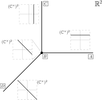
Figure 1: The fine tropical line $\operatorname{ftrop}(V(P))$ from Example 5.2. We view the ambient space $({\vmathbb C}\rtimes{\vmathbb R})^{2}$ as ${\vmathbb R}^{2}$ with a copy of $({\vmathbb C}^{\times})^{2}$ at each point. As such, $\operatorname{ftrop}(V(P))$ can be viewed as the usual tropical line in ${\vmathbb R}^{2}$ with a subvariety of the complex torus attached at each point. The labels allow identification with the components given in (5.2) and (10).

Remark 5.3.

Recall that the field of Puiseux series ${\vmathbb C}\{\!\{t\}\!\}$ also carries a fine valuation whose image is ${\vmathbb C}\rtimes{\vmathbb Q}$. Hence we can define fine tropical varieties for ideals over the Puiseux series in the space $({\vmathbb C}\rtimes{\vmathbb Q})^{n}$. For ordinary tropical varieties, one could take the closure in the Euclidean topology to view the variety in ${\vmathbb R}^{n}$ rather than ${\vmathbb Q}^{n}$. However, there are a number of topological concerns when doing this, especially outside of the setting of ordinary tropical geometry: see [27] for a discussion of pitfalls in the higher rank setting as an example. As such, we will only view fine tropical varieties over the Puiseux series in the space $({\vmathbb C}\rtimes{\vmathbb Q})^{n}$.

The remainder of this section will discuss some possible applications of fine tropical varieties as motivation for their further study.

5.1 Stable intersections

A fundamental aspect of tropical geometry is that the intersection of two tropical varieties may not be a tropical variety. Stable intersection turns out to be the correct notion of intersection, where one perturbs the tropical varieties before intersecting them. Formally, it is defined as

$$\operatorname{trop}(V(I))\wedge\operatorname{trop}(V(J))=\lim_{\epsilon\rightarrow 0}\left(\operatorname{trop}(V(I))\cap(\operatorname{trop}(V(J))+\epsilon{\bm{v}})\right)$$

for some generic vector ${\bm{v}}\in{\vmathbb R}^{n}$.

In [27], a novel approach to stable intersection was introduced, where perturbation was performed in a higher rank tropical semiring, intersected set-theoretically and then projected to the usual rank one tropical semiring. In the following, we provide evidence that a similar paradigm holds by passing to a generic fine tropical variety.

Example 5.4.

Consider the bivariate polynomials

$$P =X+Y-1\,, Q =tX+(1+t^{2})Y+1\,, P,Q\in{\vmathbb C}\llbracket t^{{\vmathbb R}}\rrbracket[X,Y]\,.$$

Their corresponding hypersurfaces $V(P),V(Q)$ are lines in the plane, and so their intersection is a single point, namely

$$V(P)\cap V(Q)=\left(\frac{2+t^{2}}{1-t+t^{2}},\frac{-1-t}{1-t+t^{2}}\right)=\left(2+2t+t^{2}+O(t^{3}),-1-2t-t^{2}+O(t^{3})\right)\in{\vmathbb C}\llbracket t^{{\vmathbb R}}\rrbracket^{2}\,.$$

Naively, we would expect the intersection of their tropical hypersurfaces to be the single point $(0,0)$. However, this is not the case as Figure 2 demonstrates: their intersection is a one-dimensional ray, but their stable intersection is the correct point,

$$\operatorname{trop}(V(P))\cap\operatorname{trop}(V(Q))=\{(g,0)\mid g\geq 0\}\,,\quad\operatorname{trop}(V(P))\wedge\operatorname{trop}(V(Q))=\{(0,0)\}\,.$$

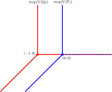
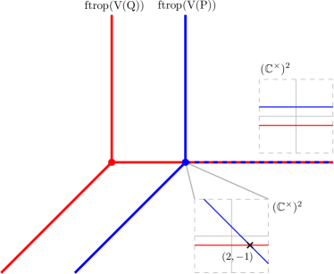
Figure 2: Left: The tropical hypersurfaces $\operatorname{trop}(V(P))$ and $\operatorname{trop}(V(Q))$ from Example 5.4. Note that they intersect in a 1-dim ray, but they intersect stably at a single point.
Right: The fine tropical hypersurfaces $\operatorname{ftrop}(V(P))$ and $\operatorname{ftrop}(V(Q))$ from the same example. These do intersect transversally, and so they intersect at a single point.

Instead let us consider their fine tropical hypersurfaces: $\operatorname{ftrop}(V(P))$ was computed in Example 5.2, and $\operatorname{ftrop}(V(Q))$ is computed analogously:

$$\operatorname{ftrop}(V(P)) =\left\{\left.\big{(}(c_{X},g_{X})\;,\,(c_{Y},g_{Y})\big{)}\in({\vmathbb C}\rtimes{\vmathbb R})^{2}\vphantom{\begin{array}[]{l}g_{X}>g_{Y}=0\,,\,c_{Y}-1=0\\ g_{Y}>g_{X}=0\,,\,c_{X}-1=0\\ g_{X}=g_{Y}<0\,,\,c_{X}+c_{Y}=0\\ g_{X}=g_{Y}=0\,,\,c_{X}+c_{Y}-1=0\end{array}}\ \right|\ \begin{array}[]{l}g_{X}>g_{Y}=0\,,\,c_{Y}-1=0\\ g_{Y}>g_{X}=0\,,\,c_{X}-1=0\\ g_{X}=g_{Y}<0\,,\,c_{X}+c_{Y}=0\\ g_{X}=g_{Y}=0\,,\,c_{X}+c_{Y}-1=0\end{array}\vphantom{\big{(}(c_{X},g_{X})\;,\,(c_{Y},g_{Y})\big{)}\in({\vmathbb C}\rtimes{\vmathbb R})^{2}}\right\}$$

$$\operatorname{ftrop}(V(Q)) =\left\{\left.\big{(}(c_{X},g_{X})\;,\,(c_{Y},g_{Y})\big{)}\in({\vmathbb C}\rtimes{\vmathbb R})^{2}\vphantom{\begin{array}[]{l}g_{X}>-1\,,\,g_{Y}=0\,,\,c_{Y}+1=0\\ g_{X}=-1\,,\,g_{Y}>0\,,\,c_{X}+1=0\\ g_{X}+1=g_{Y}<0\,,\,c_{X}+c_{Y}=0\\ g_{X}+1=g_{Y}=0\,,\,c_{X}+c_{Y}+1=0\end{array}}\ \right|\ \begin{array}[]{l}g_{X}>-1\,,\,g_{Y}=0\,,\,c_{Y}+1=0\\ g_{X}=-1\,,\,g_{Y}>0\,,\,c_{X}+1=0\\ g_{X}+1=g_{Y}<0\,,\,c_{X}+c_{Y}=0\\ g_{X}+1=g_{Y}=0\,,\,c_{X}+c_{Y}+1=0\end{array}\vphantom{\big{(}(c_{X},g_{X})\;,\,(c_{Y},g_{Y})\big{)}\in({\vmathbb C}\rtimes{\vmathbb R})^{2}}\right\}$$

It is not hard to check that these two hypersurfaces intersect at a single point $\big{(}(2,0)\;,\,(-1,0)\big{)}$. Moreover, this point is precisely $\operatorname{fval}(V(P)\cap V(Q))$, and hence its image under the projection $\omega^{\vmathbb R}\colon{\vmathbb C}\rtimes{\vmathbb R}\rightarrow{\vmathbb K}\rtimes{\vmathbb R}\cong{\vmathbb T}$ is the stable intersection of $\operatorname{trop}(V(P))$ and $\operatorname{trop}(V(Q))$, i.e.

$$\operatorname{trop}(V(P))\wedge\operatorname{trop}(V(Q))=\omega^{\vmathbb R}\left(\operatorname{ftrop}(V(P))\cap\operatorname{ftrop}(V(Q))\right)\,.$$

Observe from Figure 2 that the two rays that intersected in infinitely many points in ${\vmathbb T}$ no longer intersect at all.

Remark 5.5.

We note that moving to the fine tropical variety does not sidestep the need to perturb from all cases. For example, consider the polynomial $P^{\prime}=X+Y+1$, then

$$\operatorname{ftrop}(V(P^{\prime}))\cap\operatorname{ftrop}(V(Q))=\left\{\left.\big{(}(c_{X},g_{X})\;,\,(-1,0)\big{)}\vphantom{g_{X}>0\,,\,c_{X}\in{\vmathbb C}^{\times}}\ \right|\ g_{X}>0\,,\,c_{X}\in{\vmathbb C}^{\times}\vphantom{\big{(}(c_{X},g_{X})\;,\,(-1,0)\big{)}}\right\}\,.$$

However, we do gain two advantages from this perspective, Firstly, non-generic intersections happen less frequently for fine tropical varieties as ${\vmathbb C}\rtimes{\vmathbb R}$ is in some sense a ‘bigger’ space than ${\vmathbb T}$. Secondly, if we do need to perturb the fine tropical varieties, it suffices to only perturb in ${\vmathbb C}$ by sufficiently generic complex numbers, and leave the ‘tropical’ part as is. On the level of Hahn series, this corresponds to perturbing the leading coefficient while leaving the leading exponent be.

5.2 Polyhedral homotopies

Polyhedral homotopy continuation is a method for finding solutions to systems of polynomial equations introduced by Huber and Sturmfels [23]: we follow the tropical description in [33]. Given a polynomial system $P=(p_{1},\dots,p_{n})\subset{\vmathbb C}[X_{1},\dots,X_{n}]$ with finitely many solutions, we wish to numerically approximate $V(P)$. This is done by perturbing the coefficients of $P$ by multiplying through by $t^{\gamma}$ for various generic $\gamma\in{\vmathbb Q}$. This gives a perturbed system of equations over the Puiseux series $P_{t}=(p_{1}(t),\dots,p_{n}(t))\subset{\vmathbb C}\{\!\{t\}\!\}[X_{1},\dots,X_{n}]$. If one can understand the solutions of $P_{t}$ around $0<t\ll 1$, then we can ‘track’ these solutions to an approximate solution of the original system $P=P_{1}$ via homotopy methods.

The method for finding an initial solution of $P_{t}$ for small $t$ is roughly as follows. By calculating the tropical variety $\operatorname{trop}(V(P_{t}))$, we obtain the leading exponents of the Puiseux series solutions. Moreover, one can also recover the leading coefficient of each solution by solving an initial ideal computation. This gives us a first-order approximation of our solution set $V(P_{t})$ which in general should be sufficient information to begin homotopy continuation. However, this computation is precisely computing the fine tropical variety $\operatorname{ftrop}(V(P_{t}))$. This motivates fine tropical varieties as a natural object to work with when doing homotopy continuation.

6 Further questions

We end with some further questions and directions for study.

Theorem 4.4 gives a fundamental theorem for RAC maps from fields to hyperfields. As discussed previously, extending this statement to RAC maps between hyperfields is currently not possible due to no coherent notion of a polynomial ideal for general hyperfields. As such, the following question would have to be addressed before on could extend the fundamental theorem further:

Question 6.1.

Can one formulate a natural notion of a polynomial ideal $I\subseteq{\vmathbb H}[X_{1},\dots,X_{n}]$ over certain well-behaved ${\vmathbb H}$?

Over ${\vmathbb T}$, Maclagan and Rincón [38, 39] introduced the notion of a tropical ideal which has an additional monomial elimination axiom, similar to vector elimination axioms for matroids that occur for polynomial ideals over ${\vmathbb F}$. This axiom allows one to consider tropical ideals as compatible ‘layers’ of matroids over ${\vmathbb T}$. One possible approach is to generalise this notion to a wider family of hyperfields, where ${\vmathbb H}$-ideals are compatible layers of matroids over ${\vmathbb H}$, in the sense of [10]. Note that not all hyperfields satisfy vector elimination axioms [7], so this technique will not hold in full generality, but perhaps given coherent notions of ideals for natural families of hyperfields.

As another direction of generalisation, we use the relatively algebraically closed property to prove Kapranov’s theorem (Theorem 4.1). However, this is a stronger property than we may actually require. As an example, consider the absolute value map from the complex numbers to the triangle hyperfield:

$$|\cdot|\colon{\vmathbb C} \rightarrow\Delta=({\vmathbb R}_{\geq 0},\boxplus,\odot) a\boxplus b =\left\{\left.c\vphantom{|a-b|\leq c\leq a+b}\ \right|\ |a-b|\leq c\leq a+b\vphantom{c}\right\}$$

$$z \mapsto|z| a\odot b =a\cdot b$$

This is a hyperfield homomorphism that is not RAC. However, it was shown in [47] that Kapranov’s theorem does hold in this setting. The difference is one cannot just consider the polynomial $p$, but rather the whole principal ideal $\langle p\rangle$, as there are many ‘higher polynomials’ that contain information that $p$ does not. This motivates the following:

Question 6.2.

For which maps $f\colon{\vmathbb F}\rightarrow{\vmathbb H}$ do we have $f(V(\langle p\rangle))=V(f_{*}\langle p\rangle)$?

As with Theorem 4.4, this restricts us to maps from fields until we have a good handle on which hyperfields have well-defined notions of (principal) ideals.

Finally, note that in Theorem 4.4 we do not give any conditions on ${\vmathbb H}$ aside from it is the target of a RAC map from an algebraically closed field. In practice, all examples of such hyperfields that we know about are stringent.

Question 6.3.

Classify all hyperfields ${\vmathbb H}$ that are the target of a relatively algebraically closed map from a field. Is ${\vmathbb H}$ necessarily stringent?

The connection between RAC maps and the multiplicity bound (Definition 3.10) was investigated in [43], in particular to derive some sufficient conditions for a map to be RAC. However, if the RAC map is from a field, it may be necessary that the target hyperfield satisfies the multiplicity bound. Key examples of non-stringent hyperfields, such as ${\vmathbb P}$ and $\Delta$, are known to exceed the multiplicity bound. As such, one avenue to investigate this question is to verify whether non-stringent hyperfields exceed the multiplicity bound in general.

References

- [1] Alexander Agudelo and Oliver Lorscheid. Factorizations of tropical and sign polynomials. Indagationes Mathematicae, 32(4):797–812, 2021.
- [2] Marianne Akian, Stéphane Gaubert, and Alexander Guterman. Linear independence over tropical semirings and beyond. Contemporary Mathematics, 495(1):1–38, 2009.
- [3] Marianne Akian, Stéphane Gaubert, and Alexander Guterman. Tropical Cramer determinants revisited. Tropical and idempotent mathematics and applications, 616:1–45, 2014.
- [4] Marianne Akian, Stéphane Gaubert, and Louis Rowen. Semiring systems arising from hyperrings. arXiv preprint arXiv:2207.06739, 2022.
- [5] Marianne Akian, Stéphane Gaubert, and Hanieh Tavakolipour. Factorization of polynomials over the symmetrized tropical semiring and Descartes’ rule of sign over ordered valued fields. arXiv preprint arXiv:2301.05483, 2023.
- [6] Xavier Allamigeon, Stéphane Gaubert, and Mateusz Skomra. Tropical spectrahedra. Discrete Comput. Geom., 63(3):507–548, 2020.
- [7] Laura Anderson. Vectors of matroids over tracts. J. Combin. Theory Ser. A, 161:236–270, 2019.
- [8] Laura Anderson and James F Davis. Hyperfield Grassmannians. Advances in Mathematics, 341:336–366, 2019.
- [9] Matt Baker and Nathan Bowler. Matroids over hyperfields. In AIP Conference Proceedings, volume 1978, page 340010. AIP Publishing LLC, 2018.
- [10] Matthew Baker and Nathan Bowler. Matroids over partial hyperstructures. Advances in Mathematics, 343:821–863, 2019.
- [11] Matthew Baker and Oliver Lorscheid. Descartes’ rule of signs, Newton polygons, and polynomials over hyperfields. J. Algebra, 569:416–441, 2021.
- [12] Milo Bogaard. Introduction to amoebas and tropical geometry. PhD thesis, U. Amsterdam, 2015.
- [13] Nathan Bowler and Ting Su. Classification of doubly distributive skew hyperfields and stringent hypergroups. Journal of Algebra, 574:669–698, 2021.
- [14] David Cox, John Little, and Donal O’Shea. Ideals, varieties, and algorithms: an introduction to computational algebraic geometry and commutative algebra. Springer Science & Business Media, 2013.
- [15] Timo de Wolff. Amoebas and their tropicalizations – a survey. Analysis Meets Geometry: The Mikael Passare Memorial Volume, pages 157–190, 2017.
- [16] Andreas W. M. Dress. Duality theory for finite and infinite matroids with coefficients. Adv. in Math., 59(2):97–123, 1986.
- [17] Jens Forsgård. Tropical aspects of real polynomials and hypergeometric functions. PhD thesis, Stockholm University, 2015.
- [18] Jens Forsgård. Discriminant amoebas and lopsidedness. J. Commut. Algebra, 13(1):41–60, 2021.
- [19] Stéphane Gaubert. Theory of Linear Systems over Dioids. PhD thesis, Thèse de l’Ecole Nationale Supérieure des Mines de Paris, 1992.
- [20] Jeffrey Giansiracusa, Jaiung Jun, and Oliver Lorscheid. On the relation between hyperrings and fuzzy rings. Beiträge zur Algebra und Geometrie/Contributions to Algebra and Geometry, 58:735–764, 2017.
- [21] Andreas Gross and Trevor Gunn. Factoring multivariate polynomials over hyperfields and the multivariable Descartes’ problem. arXiv preprint arXiv:2307.09400, 2023.
- [22] Trevor Gunn. Tropical extensions and Baker-Lorscheid multiplicities for pastures. arXiv preprint arXiv:2211.06480, 2022.
- [23] Birkett Huber and Bernd Sturmfels. A polyhedral method for solving sparse polynomial systems. Math. Comp., 64(212):1541–1555, 1995.
- [24] Zur Izhakian. Tropical arithmetic and matrix algebra. Communications in Algebra, 37(4):1445–1468, 2009.
- [25] Zur Izhakian, Manfred Knebusch, and Louis Rowen. Layered tropical mathematics. Journal of Algebra, 416:200–273, 2014.
- [26] Philipp Jell, Claus Scheiderer, and Josephine Yu. Real tropicalization and analytification of semialgebraic sets. International Mathematics Research Notices, 2022(2):928–958, 2022.
- [27] Michael Joswig and Ben Smith. Convergent Hahn series and tropical geometry of higher rank. Journal of the London Mathematical Society, 107(4):1450–1481, 2023.
- [28] Jaiung Jun. Algebraic geometry over hyperrings. Adv. Math., 323:142–192, 2018.
- [29] Jaiung Jun. Geometry of hyperfields. Journal of Algebra, 569:220–257, 2021.
- [30] Marc Krasner. Approximation des corps valués complets de caractéristique p= 0 par ceux de caractéristique 0. In Colloque d’algèbre supérieure, tenu à Bruxelles du, volume 19, pages 129–206, 1956.
- [31] Marc Krasner. A class of hyperrings and hyperfields. International Journal of Mathematics and Mathematical Sciences, 6(2):307–311, 1983.
- [32] Katarzyna Kuhlmann, Alessandro Linzi, and Hanna Stojałowska. Orderings and valuations in hyperfields. J. Algebra, 611:399–421, 2022.
- [33] Anton Leykin and Josephine Yu. Beyond polyhedral homotopies. J. Symbolic Comput., 91:173–180, 2019.
- [34] Alessandro Linzi. Notes on valuation theory for Krasner hyperfields. arXiv preprint arXiv:2301.08639, 2023.
- [35] Ziqi Liu. Examples on the sharpness of an inequality about multiplicities over hyperfields. arXiv preprint arXiv:2010.09492, 2020.
- [36] Oliver Lorscheid. The geometry of blueprints: Part i: Algebraic background and scheme theory. Advances in Mathematics, 229(3):1804–1846, 2012.
- [37] Oliver Lorscheid. Tropical geometry over the tropical hyperfield. Rocky Mountain Journal of Mathematics, 52(1):189–222, 2022.
- [38] Diane Maclagan and Felipe Rincón. Tropical ideals. Compos. Math., 154(3):640–670, 2018.
- [39] Diane Maclagan and Felipe Rincón. Varieties of tropical ideals are balanced. Adv. Math., 410:Paper No. 108713, 44, 2022.
- [40] Diane Maclagan and Bernd Sturmfels. Introduction to tropical geometry, volume 161. American Mathematical Society, 2021.
- [41] Murray Marshall. Real reduced multirings and multifields. Journal of Pure and Applied Algebra, 205(2):452–468, 2006.
- [42] James Maxwell. Generalisations of tropical geometry over hyperfields. PhD thesis, Swansea University, 2022.
- [43] James Maxwell. Generalising Kapranov’s theorem for tropical geometry over hyperfields. Journal of Algebra, 2023 (to appear).
- [44] Grigory Mikhalkin. Enumerative tropical algebraic geometry in . J. Amer. Math. Soc., 18(2):313–377, 2005.
- [45] Mounir Nisse and Mikael Passare. Amoebas and coamoebas of linear spaces. Analysis Meets Geometry: The Mikael Passare Memorial Volume, pages 63–80, 2017.
- [46] Max Plus. Linear systems in (max,+) algebra. In 29th IEEE Conference on decision and control, pages 151–156. IEEE, 1990.
- [47] Kevin Purbhoo. A nullstellensatz for amoebas. Duke Math. J., 141(1):407–445, 2008.
- [48] Louis Halle Rowen. Algebras with a negation map. European Journal of Mathematics, pages 1–77, 2021.
- [49] O. Ya. Viro. Gluing of plane real algebraic curves and constructions of curves of degrees and . In Topology (Leningrad, 1982), volume 1060 of Lecture Notes in Math., pages 187–200. Springer, Berlin, 1984.
- [50] Oleg Viro. Hyperfields for tropical geometry I. hyperfields and dequantization. arXiv preprint arXiv:1006.3034, 2010.
- [51] Oleg Viro. On basic concepts of tropical geometry. Proceedings of the Steklov Institute of Mathematics, 273(1):252–282, 2011.