Orbital Stability of Periodic Traveling Waves in the $b$-Camassa-Holm Equation

Abstract

In this paper, we identify criteria that guarantees the nonlinear orbital stability of a given periodic traveling wave solution within the b-family Camassa-Holm equation. These periodic waves exist as 3-parameter families (up to spatial translations) of smooth traveling wave solutions, and their stability criteria are expressed in terms of Jacobians of the conserved quantities with respect to these parameters. The stability criteria utilizes a general Hamiltonian structure which exists for every $b>1$, and hence applies outside of the completely integrable cases ($b=2$ and $b=3$).

1 Introduction

We study the nonlinear stability of periodic traveling wave solutions for the b-family of Camassa-Holm equations (b-CH), which is given by

(1.1) $$u_{t}-u_{txx}+(b+1)uu_{x}=bu_{x}u_{xx}+uu_{xxx}$$

where here $b\in\mathbb{R}$ is a parameter. The family of models (1.1) was derived introduced in [6, 7] by using transformations of the integrable hierarchy of KdV equations. In the modeling, the b-CH equation describes the horizontal velocity $u=u(x,t)$ for the unidirectional propagation of water waves on a free surface in shallow water over a flat bed. In the special cases $b=2$ and $b=3$ it is known that (1.1) is completely integrable via the inverse scattering transform, with $b=2$ corresponding to the well-studied Camassa-Holm equation and $b=3$ corresponding to the Degasperis-Procesi equation. Further, it is known according to various tests for integrability that the b-CH equation fails to be integrable outside of the cases $b=2$ and $b=3$: see, for example, [25, 12].

Besides being completely integrable, both the Camassa-Holm and Degasperis-Procesi equations have received a considerable amount of attention due to the fact that they admit both smooth and peaked traveling solitary and periodic waves, as well as multi-soliton type solutions. Additionally, in these integrable cases the equation (1.1) admits multiple Hamiltonian structures: the Camassa-Holm equation (corresponding to $b=2$) admits three separate Hamiltonian structures, while the Degasperis-Procesi equation admits two. Concerning the stability of smooth periodic and solitary waves, there have been multiple studies of their orbital stability by working with the conserved energy integrals in the natural energy space: see, for example, [4, 22, 9, 10] and references therein. Unfortunately, the Hamiltonian structures used in these studies are a special feature due to the completely integrability of (1.1) in the cases $b=2$ and $b=3$, and hence these results cannot be extended to more general values of $b$.

In this work, we are interested in developing an orbital stability theory for periodic traveling wave solutions of (1.1) which applies to any $b>1$. Note that the analogous work for smooth solitary wave solutions of (1.1) was recently carried out in [20, 23], where the authors utilized the Hamiltonian formulation of the b-CH equation from [5]. This particular Hamiltonian formulation is expressed in terms of the so-called momentum density $m=u-u_{xx}$ of the solution, and applies to the entire family of equations (1.1) outside of the case $b=1$. In this work, we extend the work from [20] to the case of periodic traveling waves of (1.1), which inherently constitutes a much larger family of solutions: periodic traveling waves constitute (modulo spatial translations) a 3-parameter family of solutions, while the solitary waves only constitute (again modulo spatial translations) a 1-parameter family. The higher dimensionality of the associated solution manifold introduces a number of technical challenges not encountered in the solitary wave study. We approach these challenges by using a methodology introduced in [14] in the stability analysis of periodic traveling wave solutions of the generalized KdV equations.

We also note that there have been a series of recent works on the orbital stability of periodic traveling wave solutions of (1.1) in the completely integrable cases $b=2$ and $b=2$: see [9] and [10]. While there are obviously some similarities between these and the present work, the methodology for handling the higher dimensionality of the manifold of periodic traveling waves are quite different, and we will expand upon this throughout this manuscript. Additionally, both the works [9, 10] utilize Hamiltonian structures which do not extend to general $b>1$.

The basic approach utilized in this work is by now classical, essentially being an application of the methodology formalized by Grillakis, Shatah and Strauss in [11] for the stability of nonlinear solitary waves in Hamiltonian systems. Basically, we start off by carefully studying the existence theory for periodic traveling wave solutions $u(x,t)=\varphi(x-ct)$, of period $T$ say, of (1.1). As the Hamiltonian structure associated with (1.1) is expressed solely in terms of the momentum density $m=u-u_{xx}$ of solutions of (1.1), we then encode the momentum density of our solution $\mu=\varphi-\varphi^{\prime\prime}$ as a critical point of an appropriate action functional built entirely out of conserved quantities for the b-CH flow. Using Taylor series it quickly becomes apparent that the (orbital) stability or instability of $\mu$ is intimately related to the spectral properties of the second variation of the associated action functional evaluated at $\mu$. We identify conditions on the underlying wave $T$-periodic wave $\mu$ that guarantees this second variation has exactly one negative $T$-periodic eigenvalue, a simple $T$-periodic eigenvalue at the origin (associated to the translational invariance of (1.1)), and the rest of the $T$-periodic eigenvalues are strictly positive and bounded away from zero. By now considering the notion of orbtial stability (i.e. identifying functions up to spatial translations) and the class of perturbations appropriately, we then identify a final set of conditions guaranteeing the stability of $\mu$, and hence $\varphi$, to $T$-periodic perturbations.

The outline of our paper is as follows. In Section 2 we review some basic features regarding the b-CH equation (1.1), including the Hamiltonian structure used in this work as well as the existence theory for periodic traveling wave solution of (1.1). Our main stability analysis is contained in Section 3, culminating into our main result, Theorem 2. Finally, in Appendix A we establish a technical result used in Section 3.

Acknowledgments: The authors would like to thanks Stephane Lafortune and Dmitry Pelinovsky for several helpful discussions regarding the b-CH equations. The work of both authors was partially funded by the NSF under grant DMS-2108749. MAJ was also supported by the Simons Foundation Collaboration grant number 714021.

2 Some Basic Properties of the b-CH Family

In this section, we collect some basic results regarding the b-CH equation (1.1) and its solutions.

2.1 Hamiltonian Structure and Conservation Laws

For each $b\in\mathbb{R}$ the b-CH equation (1.1) is known to be a Hamiltonian system in terms of the so-called momentum density $m=u-u_{xx}$. Since we are interested in the local dynamics about periodic traveling waves, here we restrict our discussion of the Hamiltonian formulation on the space $L^{2}_{\rm per}(0,T)$ for some $T>0$. To this end, it is straightforward to see that (1.1) can be rewritten as

(2.1) $$m_{t}+um_{x}+bmu_{x}=0$$

which, for $b\neq 1$, admits the Hamiltonian formulation

(2.2) $$\frac{dm}{dt}=J_{m}\frac{\delta E}{\delta m}$$

where here

(2.3) $$J_{m}\mathrel{\mathop{\ordinarycolon}}=\frac{-1}{b-1}(bm\partial_{x}+m_{x})(1-\partial_{x}^{2})^{-1}\partial_{x}^{-1}(b\partial_{x}m-m_{x})$$

is a (state-dependent) skew-adjoint operator on $L^{2}_{\rm per}(0,T)$ and

(2.4) $$E(m)\mathrel{\mathop{\ordinarycolon}}=\int_{0}^{T}m\leavevmode\nobreak\ dx.$$

We note that from (2.1) the functional $E(m)$ is readily seen to be a conserved quantity, commonly referred to as the mass. Additionally, it is known that for general $b\neq 0$ the b-CH equation admits two additional conserved quantities given by

(2.5) $$F_{1}(m)\mathrel{\mathop{\ordinarycolon}}=\int_{0}^{T}m^{1/b}dx\leavevmode\nobreak\ \leavevmode\nobreak\ \leavevmode\nobreak\ {\rm and}\leavevmode\nobreak\ \leavevmode\nobreak\ \leavevmode\nobreak\ F_{2}(m)\mathrel{\mathop{\ordinarycolon}}=\int_{0}^{T}\left(\frac{m_{x}^{2}}{b^{2}m^{2}}+1\right)m^{-1/b}dx.$$

We note that, in general, the above functionals are well-defined and smooth functions on the set

$$X_{T}\mathrel{\mathop{\ordinarycolon}}=\left\{m\in H^{1}_{\rm per}(0,T)\mathrel{\mathop{\ordinarycolon}}m(x)>0\leavevmode\nobreak\ \leavevmode\nobreak\ {\rm for\leavevmode\nobreak\ all}\leavevmode\nobreak\ x\in\mathbb{R}\right\}.$$

Assuming that (1.1) is well-posed on some appropriate subset of $H^{1}_{\rm per}(0,T)$, our aim is to establish criteria for the nonlinear orbital stability of $T$-periodic traveling wave solutions of the b-CH equation with respect to perturbations in $H^{1}_{\rm per}(0,T)$.

Finally, a number of Jacobian determinants will arise throughout our work. For notational simplicity, we adopt the following notation for $2\times 2$ Jacobians

$$\{f,g\}_{x,y}\mathrel{\mathop{\ordinarycolon}}=\matrixdeterminant{\begin{matrix}f_{x}&f_{y}\\ g_{x}&g_{y}\end{matrix}}$$

and similarly $\{f,g,h\}_{x,y,z}$ for the analogous $3\times 3$ Jacobian.

2.2 Existence of Periodic Traveling Waves

We now study the existence of smooth periodic traveling wave solutions of (1.1). We note that the existence theory for smooth solitary wave solutions has been worked out in detail in [20]. The difference here, of course, is that the profile now does not have a constant asymptotic state as $x\to\pm\infty$.

Traveling wave solutions of (1.1) correspond to solutions of the form $u(x,t)=\varphi(x-ct)$ for some wave profile $\varphi$ and wave speed $c>0$. The profile $\varphi(z)$ is thus required to be a stationary solution of the evolutionary equation

(2.6) $$u_{t}-u_{tzz}-cu_{z}+cu_{zzz}+(b+1)uu_{z}=bu_{z}u_{zz}+uu_{zzz}$$

written here in the traveling coordinate $z=x-ct$. After some rearranging, it follows that the such stationary solutions satisfy the ODE

(2.7) $$(\varphi-c)(\varphi-\varphi^{\prime\prime})^{\prime}+b\varphi^{\prime}(\varphi-\varphi^{\prime\prime})=0,$$

where here ^′ denotes differentiation with respect to $z$. Note that, by elementary bootstrapping arguments, if $\varphi$ is a $T$-periodic weak solution of (2.7) then we necessarily have $\varphi\in C^{\infty}_{\rm per}(0,T)$ provided that either $\varphi(x)<c$ or $\varphi(x)>c$ for all $x\in\mathbb{R}$. Throughout our analysis, we consider only solutions satisfying

(2.8) $$\varphi(x)<c\leavevmode\nobreak\ \leavevmode\nobreak\ {\rm for\leavevmode\nobreak\ all}\leavevmode\nobreak\ \leavevmode\nobreak\ x\in\mathbb{R}.$$

With this condition in mind, we note that, by multiplying both sides of (2.7) by the integrating factor $(c-\varphi)^{b}$, the ODE (2.7) can be rewritten as

(2.9) $$\frac{d}{dx}\left((c-\varphi)^{b}(\varphi-\varphi^{\prime\prime})\right)=0,\leavevmode\nobreak\ \leavevmode\nobreak\ {\rm i.e.}\leavevmode\nobreak\ \leavevmode\nobreak\ \varphi-\varphi^{\prime\prime}=\frac{a}{(c-\varphi)^{b}}$$

where here $a\in\mathbb{R}$ is a constant of integration. The above may be further reduced by quadrature to

(2.10) $$\frac{1}{2}\left(\varphi^{\prime}\right)^{2}=E-\left(-\frac{1}{2}\varphi^{2}+\frac{a}{(b-1)(c-\varphi)^{b-1}}\right),$$

and hence the existence and non-existence of bounded solutions of (2.7) can be determined by studying the potential function

$$V(\varphi;a,c)\mathrel{\mathop{\ordinarycolon}}=-\frac{1}{2}\varphi^{2}+\frac{a}{(b-1)(c-\varphi)^{b-1}}.$$

Indeed, by standard phase-plane analysis it is clear that a necessary and sufficient condition for the existence of periodic solutions of (2.7) is that the potential $V(\cdot;a,c)$ have a local minimum.

Remark 1.

It is also possible to integrate the third order profile equation (2.7) directly, yielding

$$(c-\varphi)(\varphi-\varphi^{\prime\prime})+\frac{b-1}{2}\left((\varphi^{\prime})^{2}-\varphi^{2}\right)=f$$

or, equivalently,

$$-(c-\varphi)\varphi^{\prime\prime}+c\varphi+\frac{b-1}{2}\left(\varphi^{\prime}\right)^{2}-\frac{b+1}{2}\varphi^{2}=f$$

for some constant $f\in\mathbb{R}$. Using (2.9) it immediately follows that $f=(b-1)E$, with $E$ being as in (2.10), and hence, in this sense, the above equation is redundant from (2.9)-(2.10).

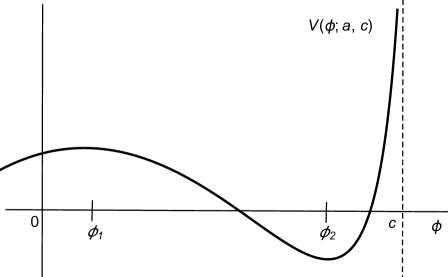
Figure 1: Depiction of the effective potential $V(\varphi;a,c)$ for an admissible value of $a$. Note there is a vertical asymptote at $\varphi=c$ and that, and that all the periodic solutions here exist for $\varphi<c$.

To study the critical points of $V$ satisfying (2.8) we note that

$$V_{\varphi}(\varphi;a,c)=-\varphi+\frac{a}{(c-\varphi)^{b}}$$

and hence seeking critical points of $V(\cdot;a,c)$ with $\varphi<c$ for fixed parameters $(a,c)$ is equivalent to seeking roots of the function

$$g(\varphi)\mathrel{\mathop{\ordinarycolon}}=\varphi(c-\varphi)^{b}-a,\leavevmode\nobreak\ \leavevmode\nobreak\ \varphi<c.$$

To this end, note that

$$g^{\prime}(\varphi)=(c-\varphi)^{b-1}\left(c-(b+1)\varphi\right)$$

and hence the only critical point of $g$ satisfying $\varphi<c$ is $\varphi=\frac{c}{b+1}$. In particular, elementary calculations show that

$$g^{\prime\prime}\left(\frac{c}{b+1}\right)=-bc\left(\frac{bc}{b+1}\right)^{b-2}<0$$

and hence $\varphi=\frac{c}{b+1}$ is a strict local maximum of $g$. Since $g\in C^{\infty}(-\infty,c)$ it follows by above that $g$ is strictly increasing on $\left(-\infty,\frac{c}{b+1}\right)$ and strictly decreasing on $\left(\frac{c}{b+1},c\right)$. Further, we have

$$g(0)=-a,\leavevmode\nobreak\ \leavevmode\nobreak\ g\left(\frac{c}{b+1}\right)=\frac{b^{b}c^{b+1}}{(b+1)^{b+1}}-a,\leavevmode\nobreak\ \leavevmode\nobreak\ \lim_{\varphi\to c}g(\varphi)=-a$$

and hence, by the Intermediate Value Theorem, for each $a\in\left(0,\frac{b^{b}c^{b+1}}{(b+1)^{b+1}}\right)$ the equation $g(\varphi)=0$ has exactly two solutions $\varphi_{1}\in\left(0,\frac{c}{b+1}\right)$ and $\varphi_{2}\in\left(\frac{c}{b+1},c\right)$. For such $a$ we necessarily have $V^{\prime}(\varphi_{1})=V^{\prime}(\varphi_{2})=0$ and, since

$$V_{\varphi}(\varphi;a,c)=-\frac{g(\varphi)}{(c-\varphi)^{b}},$$

it follows that $V$ achieves unique local max and min values at $\varphi_{1}$ and $\varphi_{2}$, respectively.

It follows by the above and elementary phase plane analysis that if we define the set

(2.11) $$\mathcal{B}\mathrel{\mathop{\ordinarycolon}}=\left\{(a,E,c)\in\mathbb{R}^{3}\mathrel{\mathop{\ordinarycolon}}c>0,\leavevmode\nobreak\ \leavevmode\nobreak\ a\in\left(0,\frac{b^{b}c^{b+1}}{(b+1)^{(b+1)}}\right),\leavevmode\nobreak\ \leavevmode\nobreak\ E\in\left(V(\varphi_{2};a,c),V(\varphi_{1};a,c)\right)\right\}$$

then for each set of parameters $(a,E,c)\in\mathcal{B}$ the profile equation (2.7) admits a one-parameter family, parameterized by translation invariance, of smooth periodic solutions $\varphi(x;a,E,c)$ satisfying $\varphi<c$ and with period

$$T=T(a,E,c)=\sqrt{2}\int_{\varphi_{\rm min}}^{\varphi_{\rm max}}\frac{d\varphi}{\sqrt{E-V(\varphi;a,c)}},$$

where here $\varphi_{\rm min}$ and $\varphi_{\rm max}$ denote, respectively, the minimum and maximum roots of the equation $E-V(\cdot;a,c)=0$, respectively, and hence correspond to the minimum and maximum values of the corresponding periodic solution $\varphi$. Note that since the values $\varphi_{\rm min}$ and $\varphi_{\rm max}$ are smooth functions of the traveling wave parameters $(a,E,c)$, it follows that the period function $T(a,E,c)$ represents a $C^{1}$ function on $\mathcal{B}$.

Putting all of the above together, it follows that the b-CH equation (1.1) admits a 4-parameter family, constituting a $C^{1}$ manifold, of periodic traveling wave solutions of the form

$$\varphi(x-ct+x_{0};a,E,c),\leavevmode\nobreak\ \leavevmode\nobreak\ x_{0}\in\mathbb{R},\leavevmode\nobreak\ \leavevmode\nobreak\ (a,E,c)\in\mathcal{B}$$

with period $T=T(a,E,c)$. Recalling from the previous section that the Hamiltonian formulation for the b-CH equation is expressed entirely in terms of the momentum density $m=u-u_{xx}$, we note from (2.9) that if $\varphi(x;a,E,c)$ is a smooth $T$-periodic stationary solution (2.6) as constructed above, then

(2.12) $$\mu(x;a,E,c)=\frac{a}{(c-\varphi(x;a,E,c))^{b}}$$

is a smooth $T$-periodic stationary solution of

$$m_{t}-cm_{x}+um_{x}+bmu_{x}=0$$

satisfying $\mu>0$ for all $x\in\mathbb{R}$. In particular, for each $(a,E,c)\in\mathcal{B}$ we have $\mu(x;a,E,c)\in X_{T}$ with $T=T(a,E,c)$. Further, following the procedure above we can restrict the conserved quantities in (2.5) to the manifold of periodic traveling wave solutions of the b-CH equation yielding, with slight abuse of notation, $C^{1}$ functions $F_{1},F_{2}\mathrel{\mathop{\ordinarycolon}}\mathcal{B}\to\mathbb{R}$ defined via

$$\left\{\begin{aligned} F_{1}(a,E,c)&\mathrel{\mathop{\ordinarycolon}}=\int_{0}^{T(a,E,c)}\mu(x;a,E,c)^{1/b}dx\\ F_{2}(a,E,c)&\mathrel{\mathop{\ordinarycolon}}=\int_{0}^{T(a,E,c)}\left(\frac{\mu_{x}(x;a,E,c)^{2}}{b^{2}\mu(x;a,E,c)^{2}}+1\right)\mu(x;a,E,c)^{-1/b}dx\end{aligned}\right.$$

As we will see, the gradients of these conserved quantities along the manifold of periodic traveling wave solutions of (1.1), or equivalently (2.1), will plan a central role in our forthcoming analysis.

Remark 2.

As mentioned in the introduction, there are similarities between the present work and that in [9, 10], where authors considered the stability of periodic traveling wave solutions of the b-CH equation (1.1) in the completley integrable cases $b=2$ and $b=3$. In addition to using a different Hamiltonian structure in our work (recall those used in [9, 10] do not extend outside the completely integrable cases), our work differs in how we parameterize the set of periodic traveling waves. In [9, 10], the authors, for a fixed $b>1$, start by fixing a $c>0$ and thus reducing to a 2-parameter family depending on $(a,E)$. They then consider a curve $E=E(a)$ in parameter space where the period is held constant, and thus reduce to a 1-parameter family of waves with a fixed period and fixed wave speed depending only on the parameter $a$. In our work, by contrast, we work with the full 4-parameter family of periodic traveling waves and their variations with respect to all four parameters. This results in the introduction of a number of Jacobian determinants associated with this parameterization arising in our work, which of course are geometrically related to the ability to locally reparameterize the manifold of solutions. This geometric/Jacobian approach has had significant success not only in orbital stability analysis of periodic traveling waves in nonlinear dispersive systems, but also in the stability analysis of such solutions to more general classes of perturbations. See, for example, [14, 2, 15, 18, 17, 3, 1, 13, 16].

3 Orbital Stability Criteria

In this section, we derive conditions which guarantee a given $T$-periodic traveling wave solution of the b-CH equation is orbitally stable with respect to $T$-periodic perturbations. Throughout our analysis, we will work in the momentum density formulation (2.1),. To this end, we begin by attempting to encode a given $T$-periodic traveling wave solution $\mu(\cdot;a,E,c)$ as a critical point of an action functional of the form

(3.1) $$\Lambda(m)=E(m)-\omega_{1}F_{1}(m)-\omega_{2}F_{2}(m),\leavevmode\nobreak\ \leavevmode\nobreak\ \omega_{1},\omega_{2}\in\mathbb{R}$$

defined when $m\in H_{per}^{1}[0,T]$ and $m>0$, where here $E$ denotes the mass functional (2.4) and $F_{1},F_{2}$ are the conserved quantities given in (2.5). More specifically, we seek values $\omega_{1},\omega_{2}\in\mathbb{R}$ such that the profile equation (2.10) is equivalent to the Euler-Lagrange equation of the functional $\Lambda$. This is accomplished in the following Lemma.

Lemma 1.

For a fixed $b>1$, let $\mu(\cdot;a,E,c)$ be a $T$-periodic solution of (2.10). Then $\mu$ is a critical point of the action functional $\Lambda(m)$ provided that

$$\omega_{1}=\frac{1}{2a^{\frac{1}{b}}}\left[2(b-1)E+(b-1)c^{2}\right]\leavevmode\nobreak\ \leavevmode\nobreak\ {\rm and}\leavevmode\nobreak\ \leavevmode\nobreak\ \omega_{2}=\frac{1}{2}a^{\frac{1}{b}}(b-1)$$

Proof.

The proof is given in [20, Lemma 2]. For completeness, we outline the main idea of the argument. First, from (2.5) we note that

$$\frac{\partial E}{\partial m}=1,\leavevmode\nobreak\ \leavevmode\nobreak\ \leavevmode\nobreak\ \leavevmode\nobreak\ \frac{\partial F_{1}}{\partial m}(m)=\left(\frac{1}{b}\right)m^{1/b-1}$$

and

$$\frac{\partial F_{2}}{\partial m}(m)=\frac{1}{b}m^{-(1/b+1)}\left(\frac{(2b+1)m_{x}^{2}}{b^{2}m^{2}}-\frac{2m_{xx}}{bm}-1\right).$$

and hence the equation $\frac{\partial\Lambda}{\partial m}(\mu)=0$ is equivalent to the differential equation

(3.2) $$1-\omega_{1}\left(\frac{1}{b}\right)\mu^{\frac{1}{b}-1}-\omega_{2}\frac{1}{b}\mu^{\frac{-1}{b}-1}\left(\frac{(2b+1)\mu_{x}^{2}}{b^{2}\mu^{2}}-\frac{2\mu_{xx}}{b\mu}-1\right)=0$$

As in [20], we note that if $\mu$ is a $T$-periodic weak solution of (3.2) then by elementary bootstrapping arguments we have $\mu\in C^{\infty}_{\rm per}(0,T)$. Consequently, to show the critical points of $\Lambda$ are precisely the periodic traveling wave solutions $\mu(\cdot;a,E,c)$ constructed in the previous section, it is sufficient to establish an equivalence between the differential equation (3.2) and (2.9).

To this end, it is important to observe that differentiating (2.9) one has the relations

(3.3) $$\mu^{\prime}=\frac{b\varphi^{\prime}}{c-\varphi}\mu\leavevmode\nobreak\ \leavevmode\nobreak\ {\rm and}\leavevmode\nobreak\ \leavevmode\nobreak\ \mu^{\prime\prime}=\frac{b\varphi^{\prime\prime}}{c-\varphi}\mu+\frac{b(b+1)\left(\varphi^{\prime}\right)^{2}}{(c-\varphi)^{2}}\mu$$

and hence derivatives of $\mu$ in (3.2) can be replaced by derivatives of $\varphi$ and multiples of $\mu$. Upon making these substitutions into (3.2) one finds by straightforward calculations that the resulting equation is equivalent to (2.10) provided the stated choices of $\omega_{1}$ and $\omega_{2}$ are made. For more details, see [20]. ∎

Remark 3.

It is important to note that the Lagrange multipliers $\omega_{1}$ and $\omega_{2}$ found above are smooth functions of the traveling wave parameters $(a,E,c)$ on the entire existence set $\mathcal{B}$ defined in (2.11). In particular, we note that

$$\nabla_{(a,E,c)}\omega_{1}=\left<\frac{-1}{2ba^{\frac{1}{b}+1}}\left[2(b-1)E+(b-1)c^{2}\right],\leavevmode\nobreak\ \frac{b-1}{a^{\frac{1}{b}}},\leavevmode\nobreak\ \frac{c(b-1)}{a^{1/b}}\right>$$

and

$$\nabla_{(a,E,c)}\omega_{2}=\left<\frac{1}{2b}a^{\frac{1}{b}-1}\left(b-1\right),\leavevmode\nobreak\ 0,\leavevmode\nobreak\ 0\right>.$$

In particular, while $\omega_{2}$ depends only on the parameter $a$, the Lagrange multiplier $\omega_{1}$ depends on all three traveling wave parameters $(a,E,c)$. This is a quite different case than that encountered, say, in the KdV, BBM or NLS type equations where each Lagrange multiplier depends on only one of the traveling wave parameters: see, for instance, [14, 15, 8, 21]. In the forthcoming analysis, it is interesting to track the effect of this additional dependence of the Lagrange multipliers.

By Lemma 1, our periodic traveling wave solutions $\mu(\cdot;a,E,c)$ of the b-CH equation are realized as critical points of the action functional $\Lambda$. In order to classify this critical point as a local minimum, maximum or a saddle point, we study the second derivative

$$\mathcal{L}[\mu]\mathrel{\mathop{\ordinarycolon}}=\frac{\delta^{2}\Lambda}{\delta^{2}m}(\mu)$$

evaluated at the wave $\mu(\cdot;a,E,c)$. To this end, we note through straightforward, but lengthy and tedious, calculations (see, for example, [20, Corollary 1]) the operator $\mathcal{L}[\mu]$ can be expressed as a Sturm-Liouville operator of the form

(3.4) $$\mathcal{L}[\mu]=-p(x)\partial_{x}^{2}-q(x)\partial_{x}-r(x)$$

where $p$, $q$, and $r$ are smooth, $T$-periodic functions with

(3.5) $$p(x)=\frac{\omega_{2}}{b^{2}\mu^{2+1/b}},\leavevmode\nobreak\ \leavevmode\nobreak\ \leavevmode\nobreak\ q(x)=-\frac{\omega_{2}(2b+1)\mu_{x}}{b\mu^{3+1/b}}.$$

In particular, we note, since $b>1$, that $p(x)>0$ for all $x\in\mathbb{R}$.

It follows that $\mathcal{L}[\mu]$ is a self-adjoin linear operator acting on $L^{2}_{\rm per}(0,T)$ with compactly embedded domain $H^{2}_{\rm per}(0,T)$. Consequently, it is well-known that the spectrum of $\mathcal{L}[\mu]$ on $L^{2}_{\rm per}(0,T)$ consists of an increasing sequence of real eigenvalues satisfying

$$\lambda_{0}<\lambda_{1}\leq\lambda_{2}<\lambda_{3}\leq\lambda_{4}\ldots\nearrow+\infty$$

and that the associated eigenfunctions $\{\psi_{n}\}_{n=0}^{\infty}$ forms an orthogonal basis for $L^{2}_{\rm per}(0,T)$. Further, the (ground state) eigenfunction $\psi_{0}$ can be chosen to be strictly positive, while for each $n\in\mathbb{N}$ the eigenfunctions $\psi_{2n-1}$ and $\psi_{2n}$ have precisely $2n$ simple zeroes on $[0,T)$.

Noting that, by the spatial translation invariance of (2.1), we have

$$\mathcal{L}[\mu]\mu_{x}=0$$

it follows that $\lambda=0$ is a $T$-periodic eigenvalue of $\mathcal{L}[\mu]$. Since $\mu_{x}$ has precisely two roots on $[0,T)$, by construction, it further follows that $\lambda=0$ is either the second or third smallest eigenvalue of $\mathcal{L}[\mu]$ and hence, in particular, $\mathcal{L}[\mu]$ has at least one negative eigenvalue. A precise count on the number of negative eigenvalues, as well as the simplicity of the zero eigenvalue, is established in the following result.

Theorem 1.

The spectrum of the linear operator $\mathcal{L}[\mu]$ considered on the space $L^{2}_{\rm per}(0,T)$ satisfies the following trichotomy:

• If $\{T,\omega_{1}\}_{E,c}>0$ then $\mathcal{L}[\mu]$ has exactly one negative eigenvalue, a simple eigenvalue at zero, and the rest of the spectrum is strictly positive and bounded away from zero.

• If $\{T,\omega_{1}\}_{E,c}=0$ then $\mathcal{L}[\mu]$ has exactly one negative eigenvalue, a double eigenvalue at zero, and the rest of the spectrum is strictly positive and bounded away from zero.

• If $\{T,\omega_{1}\}_{E,c}<0$ then $\mathcal{L}[\mu]$ has exactly two negative eigenvalues, a simple eigenvalue at zero, and the rest of the spectrum is strictly positive and bounded away from zero.

The general strategy for the proof is similar to that given in [9, Theorem 4], and relies on a well-known result from Floquet theory as well as Sylvester’s Inertial Law theorem. Before we proceed with the proof of Theorem 1, we state these auxiliary results.

Lemma 2.

[26] Consider the Schrödinger operator $\mathcal{M}=-\partial_{x}^{2}+Q(x)$ with an even, $T$-periodic, smooth potential $Q$. Assume that there exists linearly independent functions $\varphi_{1},\varphi_{2}\in L^{2}_{\rm per}(0,T)$ that are solutions of $\mathcal{M}w=0$ and such that there exists constant $\theta\in\mathbb{R}$ such that

$$\varphi_{1}(x+T)=\varphi_{1}(x)+\theta\varphi_{2}(x)\leavevmode\nobreak\ \leavevmode\nobreak\ {\rm and}\leavevmode\nobreak\ \leavevmode\nobreak\ \varphi_{2}(x+T)=\varphi_{2}(x).$$

Further, suppose that $\varphi_{2}$ has two zeros on $[0,T)$. The zero eigenvalue of $\mathcal{M}$ is simple if $\theta\neq 0$ and double if $\theta=0$. Furthermore, $\mathcal{M}$ has one negative eigenvalue if $\theta\geq 0$ and two negative eigenvalues if $\theta<0$.

Lemma 3 (Sylvester’s Inertial Law [24]).

Let $L$ be a self-adjoint operator on a Hilbert space $H$, and let $\mathcal{S}$ be a bounded, invertible operator on $H$. Then the operators $L$ and $\mathcal{S}L\mathcal{S}^{*}$ have the same inertia, i.e. the dimensions of the negative, null, and positive invariant subspaces of $H$ for these two operators are the same.

With these results in hand, we now establish Theorem 1.

Proof of Theorem 1.

The basic strategy, which again is similar to that in [9], is to first show that the Sturm-Liouville operator $\mathcal{L}[\mu]$ can be written as

$$\mathcal{L}[\mu]=\mathcal{S}\mathcal{M}\mathcal{S}^{*}$$

for some linear Schrödinger operator $\mathcal{M}$ (as in Lemma 2 above) and some bounded, invertible operator $\mathcal{S}$ (as in Lemma 3 above). To this end, first note by (3.4) the spectral problem $\mathcal{L}[\mu]v=\lambda v$ can be written as

$$p(x)v^{\prime\prime}+q(x)v^{\prime}+\left(r(x)+\lambda\right)=0.$$

We now define the function

$$D(x)=\int_{0}^{x}\frac{q(s)}{p(s)}ds=\ln\left(\left(\frac{c-\varphi(x)}{c-\varphi(0)}\right)^{-(2b+1)}\right)$$

and making the change of variables

(3.6) $$v(x)=w(x)e^{-D(x)/(4b+2)}$$

a straightforward calculation shows that

$$-w^{\prime\prime}+Q(x)w=\lambda(c-\varphi)^{-1}w,$$

where here $Q$ is smooth, $T$-periodic and even.

Defining the linear Schrödinger operator $\mathcal{M}\mathrel{\mathop{\ordinarycolon}}=-\partial_{x}^{2}+Q(x)$ and defining the multiplication operator $\mathcal{S}\mathrel{\mathop{\ordinarycolon}}=(c-\varphi)^{1/2}$, which is clearly bounded and invertible, it follows that $\lambda\in\mathbb{R}$ is an eigenvalue of $\mathcal{L}[\mu]$ if and only if it is an eigenvalue of $\mathcal{S}\mathcal{M}\mathcal{S}^{*}$. By Sylverster’s inertial law theorem it follows that $\mathcal{S}\mathcal{M}\mathcal{S}^{*}$, and by extension $\mathcal{L}[\mu]$, necessarily has the same inertia as the operator $\mathcal{M}$.

It remains to determine the inertia of the operator $\mathcal{M}$. To this end, we aim to build functions $\varphi_{1}$ and $\varphi_{2}$ as in Lemma 2 by first building corresponding functions for the operator $\mathcal{L}[\mu]$. First, notice that $\mathcal{L}[\mu]\mu_{x}=0$ and

$$\mathcal{L}[\mu]\mu_{E}=\frac{\partial\omega_{1}}{\partial E}\frac{\partial F_{1}}{\partial m}(\mu),\leavevmode\nobreak\ \leavevmode\nobreak\ \mathcal{L}[\mu]\mu_{c}=\frac{\partial\omega_{1}}{\partial c}\frac{\partial F_{1}}{\partial m}(\mu),$$

where the last two relations come from differentiating the profile equation $\Lambda^{\prime}(\mu)=0$ with respect to the parameters $E$ and $c$, respectively. It follows that the functions

$$\mu_{x}\leavevmode\nobreak\ \leavevmode\nobreak\ \leavevmode\nobreak\ {\rm and}\leavevmode\nobreak\ \leavevmode\nobreak\ \leavevmode\nobreak\ \frac{\partial\omega_{1}}{\partial c}\mu_{E}-\frac{\partial\omega_{1}}{\partial E}\mu_{c}=\{\mu,\omega_{1}\}_{E,c}$$

provide two linearly independent solutions, the first being odd and the second even, of the equation $\mathcal{L}[\mu]v=0$. We now define the functions

$$y_{1}(x)=\frac{\{\mu(x),\omega_{1}\}_{E,c}}{\{\mu_{+},\omega_{1}\}_{E,c}},\leavevmode\nobreak\ \leavevmode\nobreak\ \leavevmode\nobreak\ y_{2}(x)=\frac{\mu_{x}(x)}{\mu_{xx}(0)},$$

which are well-defined thanks to the technical result in Lemma 5 (see Appendix A) and are linearly independent by parity, and note that $y_{2}$ is $T$-periodic while $y_{1}$ satisfies

(3.7) $$y_{1}(x+T)=y_{1}(x)+\theta y_{2}(x),\leavevmode\nobreak\ \leavevmode\nobreak\ \theta=y_{1}^{\prime}(T).$$

To see the above equality, note that differentiating the identity $\mu(x+T)=\mu(x)$ with respect to the parameters $E$ and $c$ gives

$$\mu_{E}(x+T)-\mu_{E}(x)=-T_{E}\mu_{x}(x),\leavevmode\nobreak\ \leavevmode\nobreak\ {\rm and}\leavevmode\nobreak\ \leavevmode\nobreak\ \mu_{c}(x+T)-\mu_{c}(x)=-T_{c}\mu_{x}(x)$$

and hence

(3.8) $$y_{1}(x+T)=y_{1}(x)+\left(\frac{\mu_{x}(x)}{\mu_{xx}(0)}\right)\left(-\mu_{xx}(0)\frac{\{T,\omega_{1}\}_{E,c}}{\{\mu_{+},\omega_{1}\}_{E,c}}\right)$$

Similarly, differentiating the relation $\mu_{x}(T)=0$ with respect to $E$ and $c$ and using the $T$-periodicity of $\mu(x)$ gives

$$\mu_{Ex}(T)=\mu_{xx}(T)T_{E}=\mu_{xx}(0)T_{E}\leavevmode\nobreak\ \leavevmode\nobreak\ \leavevmode\nobreak\ {\rm and}\leavevmode\nobreak\ \leavevmode\nobreak\ \leavevmode\nobreak\ \mu_{cx}(T)=\mu_{xx}(0)T_{c}$$

and hence

$$\theta=-\mu_{xx}(0)\frac{\{T,\omega_{1}\}_{E,c}}{\{\mu_{+},\omega_{1}\}_{E,c}},$$

which, along with (3.8), verifies (3.7). We further note that since Lemma 5 in Appendix A implies that $\mu_{xx}(0)<0$ and $\{\mu_{+},\omega_{1}\}_{E,c}>0$, it follows that

$${\rm sign}\left(\theta\right)={\rm sign}\left(\{T,\omega_{1}\}_{E,c}\right).$$

Of specific note, this shows that $y_{1}$ provides a second linearly independent solution of $\mathcal{L}[\mu]v=0$ if and only if $\{T,\omega_{1}\}_{E,c}=0$.

Now, observing from that the change of variables (3.6) that $v(0)=w(0)$ and $v^{\prime}(0)=w^{\prime}(0)$, we define

$$\varphi_{1}(x)=\left(\frac{c-\varphi}{c-\varphi\left(0\right)}\right)^{-1/2}y_{1}(x)\leavevmode\nobreak\ \leavevmode\nobreak\ {\rm and}\leavevmode\nobreak\ \leavevmode\nobreak\ \varphi_{2}(x)=\left(\frac{c-\varphi}{c-\varphi\left(0\right)}\right)^{-1/2}y_{2}(x)$$

and note that, by construction, $\varphi_{1,2}$ are linearly independent solutions of the differential equation $\mathcal{M}w=0$ and satisfy

$$\varphi_{1}(x+T)=\varphi_{1}(x)+\theta\varphi_{2}(x),\leavevmode\nobreak\ \leavevmode\nobreak\ \leavevmode\nobreak\ \varphi_{2}(x+T)=\varphi_{2}(x)$$

for all $x\in\mathbb{R}$, where $\theta$ is as in (3.7). Since $\varphi_{2}$ has precisely two roots in $[0,T)$ by construction, it follows from Lemma 2 that the zero eigenvalue of $\mathcal{M}$ is simple if and only if $\theta\neq 0$. If $\theta\neq 0$, then $\lambda=0$ is a simple eigenvalue of $\mathcal{M}$ and, again by Lemma 2, $\mathcal{M}$ has either one or two negative eigenvalues depending on whether $\theta>0$ or $\theta<0$, respectively. The proof is complete by recalling that, by Sylverster’s inertial law theorem, the operators $\mathcal{M}$ and $\mathcal{S}\mathcal{M}\mathcal{S}^{*}$, and hence $\mathcal{L}[\mu]$ by the change of variables (3.6), have the same inertia. ∎

Remark 4.

It is interesting to note that the function $y_{1}$ would be considerably simpler if if the Lagrange multiplier $\omega_{1}$ depended only one one of the traveling wave parameters $E$ or $c$. This simplification occurs in many other nonlinear dispersive equations such as the KdV type equations and even in the integrable cases $b=2$ and $b=3$ of the b-CH equation (1.1): see, for example, the works [14, 15, 3, 1, 9, 10].

Throughout the remainder of our stability analysis, we will assume

(3.9) $$\{T,\omega_{1}\}_{E,c}>0.$$

From Theorem 1 it follows that our given $T$-periodic traveling wave solution $\mu$ is a degenerate saddle point of the functional $\Lambda$ on $L^{2}_{\rm per}(0,T)$, with one unstable direction and one neutral direction. To accommodate these negative and null directions, we note that the evolution of (2.1) does not occur on all of $L^{2}_{\rm per}(0,T)$ but rather on the co-dimension two submanifold

$$\Sigma_{0}\mathrel{\mathop{\ordinarycolon}}=\left\{m\in H^{1}_{\rm per}(0,T)\mathrel{\mathop{\ordinarycolon}}F_{1}(m)=F_{1}(\mu(\cdot;a,E,c)),\leavevmode\nobreak\ \leavevmode\nobreak\ F_{2}(m)=F_{2}(\mu(\cdot;a,E,c))\right\}.$$

Further, since the evolution of (2.1) remains invariant under the one-parameter group of isometries corresponding to spatial translations, this motivates us to define the group orbit of $\mu\in\Sigma_{0}$ as

$$\mathcal{O}_{\mu}\mathrel{\mathop{\ordinarycolon}}=\left\{\mu(\cdot-x_{0})\mathrel{\mathop{\ordinarycolon}}x_{0}\in\mathbb{R}\right\}.$$

We note that $\mathcal{O}_{\mu}\subset\Sigma_{0}$ and that a solution of (2.1) with initial data in $\Sigma_{0}$ will remain in $\Sigma_{0}$ for all future times. Our strategy moving forward will be to demonstrate the “convexity” of the functional $\Lambda$ in (3.1) on the nonlinear manifold $\Sigma_{0}$ in a neighborhood of the group orbit $\mathcal{O}_{\mu}$.

To this end, we define

$$\mathcal{T}_{0}\mathrel{\mathop{\ordinarycolon}}=\left\{m\in H^{1}_{\rm per}(0,T)\mathrel{\mathop{\ordinarycolon}}\left<m,\frac{\partial F_{1}}{\partial m}(\mu)\right>=\left<m,\frac{\partial F_{2}}{\partial m}(\mu)\right>=0\right\}$$

and note that $\mathcal{T}_{0}$ is precisely the tangent space in $H^{1}_{\rm per}(0,T)$ to the submanifold $\Sigma_{0}$ at the point $\mu$. Our next result establishes the positivity of the linear operator $\mathcal{L}[\mu]$ on the tangent space $\mathcal{T}_{0}$ which are orthogonal to the kernel of $\mathcal{L}[\mu]$.

Lemma 4.

Assume that $\{T,\omega_{1}\}_{E,c}>0$ and that the product $\{T,F_{1}\}_{E,c}\{T,F_{1},F_{2}\}_{a,E,c}$ is negative. Then

$$\inf\left\{\left<\mathcal{L}[\mu]m,m\right>\mathrel{\mathop{\ordinarycolon}}\|m\|_{L^{2}_{\rm per}(0,T)}=1,\leavevmode\nobreak\ \leavevmode\nobreak\ m\in\mathcal{T}_{0},\leavevmode\nobreak\ \leavevmode\nobreak\ m\perp\mu_{x}\right\}>0.$$

In particular, there exists a constant $C>0$ such that

$$\left<\mathcal{L}[\mu]m,m\right>\geq C\|m\|_{L^{2}(0,T)}^{2}$$

for all $m\in\mathcal{T}_{0}$ with $m\perp\mu_{x}$.

Proof.

We define the function

$$\psi=\{\mu,T,F_{1}\}_{a,E,c}$$

and note that $\psi$ is smooth, $T$-periodic and satisfies

$$\mathcal{L}[\mu]\psi =\matrixdeterminant{\begin{matrix}(\omega_{1})_{a}\frac{\delta F_{1}}{\delta m}+(\omega_{2})_{a}\frac{\delta F_{2}}{\delta m}&(\omega_{1})_{E}\frac{\delta F_{1}}{\delta m}&(\omega_{1})_{c}\frac{\delta F_{1}}{\delta m}\\ T_{a}&T_{E}&T_{c}\\ (F_{1})_{a}&(F_{1})_{E}&(F_{1})_{c}\end{matrix}}$$

$$=\{\omega_{1},T,F_{1}\}_{a,E,c}\frac{\delta F_{1}}{\delta m}+(\omega_{2})_{a}\{T,F_{1}\}_{E,c}\frac{\delta F_{2}}{\delta m}.$$

In particular, we have that $\left<\mathcal{L}[\mu]\psi,m\right>=0$ for all $m\in\mathcal{T}_{0}$. Further, we have

$$\left<\mathcal{L}\psi,\psi\right> =\{\omega_{1},T,F_{1}\}_{a,E,c}\left<\frac{\delta F_{1}}{\delta m},\{\mu,T,F_{1}\}_{a,E,c}\right>$$

$$\quad+(\omega_{2})_{a}\{T,F_{1}\}_{E,c}\left<\frac{\delta F_{2}}{\delta m},\{\mu,T,F_{1}\}_{a,E,c}\right>$$

Noting that

$$\int_{0}^{T}\frac{\partial F_{j}}{\partial m}\nabla_{(a,E,c)}\mu\leavevmode\nobreak\ dx=\nabla_{(a,E,c)}F_{j}-\mu(T)\nabla_{(a,E,c)}T$$

for both $j=1,2$, we see that

$$\left<\frac{\delta F_{1}}{\delta m},\{\mu,T,F_{1}\}_{a,E,c}\right>=\{F_{1},T,F_{1}\}_{a,E,c}=0$$

and

$$\left<\frac{\delta F_{2}}{\delta m},\{\mu,T,F_{1}\}_{a,E,c}\right>=\{F_{2},T,F_{1}\}_{a,E,c}=\{T,F_{1},F_{2}\}_{a,E,c},$$

and hence

$$\left<\mathcal{L}[\mu]\psi,\psi\right>=(\omega_{2})_{a}\{T,F_{1}\}_{E,c}\{T,F_{1},F_{2}\}_{a,E,c}.$$

Since $(\omega_{2})_{a}>0$ (see Remark 3), it follows by assumption that the quantity $\left<\mathcal{L}[\mu]\psi,\psi\right>$ is negative.

Now, let $m\in\mathcal{T}_{0}$ be such that $\left<m,\mu_{x}\right>=0$. Due to Theorem 1, the assumption $\{T,\omega_{1}\}_{E,c}>0$ implies we can write $\psi=\alpha\chi+\beta\mu_{x}+p$ and $m=A\chi+\widetilde{p}$ for some constants $\alpha,\beta,A\in\mathbb{R}$, the function $\chi$ belongs to the negative invariant space for $\mathcal{L}[\mu]$ and functions $p$ and $\widetilde{p}$ belong to the positive invariant subspace of $\mathcal{L}[\mu]$. It follows then that

(3.10) $$\left<\mathcal{L}[\mu]m,m\right>=-\lambda A^{2}+\left<\mathcal{L}[\mu]\widetilde{p},\widetilde{p}\right>,$$

where here $\lambda$ is the eigenvalue associated to $\chi$. Further, we have

$$0=\left<\mathcal{L}[\mu]\psi,m\right>=-\lambda^{2}A\alpha+\left<\mathcal{L}[\mu]p,\widetilde{p}\right>$$

and

$$0>\left<\mathcal{L}[\mu]\psi,\psi\right>=-\lambda\alpha^{2}+\left<\mathcal{L}[\mu]p,p\right>$$

and hence, noting that the bilinear form $\left<\mathcal{L}[\mu]\cdot,\cdot\right>$ is an inner-product on the positive invariant subspace of $\mathcal{L}[\mu]$, an application of Cauchy-Schwarz gives

$$\left<\mathcal{L}[\mu]\widetilde{p},\widetilde{p}\right>\geq\frac{\left<\mathcal{L}[\mu]\widetilde{p},p\right>^{2}}{\left<\mathcal{L}[\mu]p,p\right>}>-\lambda A^{2}.$$

Substituting this bound into (3.10), the result now follows. ∎

Next, we upgrade the result of Lemma 4 to provide a coercivity bound in $H^{1}$.

Proposition 1.

Under the same hypotheses as Lemma 4, we have

$$\left<\mathcal{L}[\mu]m,m\right>\geq C\|m\|_{H^{1}(0,T)}^{2}$$

for all $m\in\mathcal{T}_{0}$ with $m\perp\mu_{x}$.

Proof.

This follows by an elementary interpolation argument. Indeed, recalling (3.4) and rewriting $\mathcal{L}[\mu]$ in the symmetric form

$$\mathcal{L}[\mu]=-\partial_{x}\left(p(x)\partial_{x}\right)+r(x)$$

we note that for $m\in\mathcal{T}_{0}$ with $m\perp\mu_{x}$ we have

$$\left<\mathcal{L}[\mu]m,m\right> =\int_{0}^{T}p\left(\mu_{x}\right)^{2}dx+\int_{0}^{T}r\mu^{2}\leavevmode\nobreak\ dx$$

$$\geq\alpha\int_{0}^{T}(\mu_{x})^{2}dx+\beta\int_{0}^{T}u^{2}dx,$$

where here

$$\alpha\mathrel{\mathop{\ordinarycolon}}=\inf_{0\leq x\leq T}p(x)\leavevmode\nobreak\ \leavevmode\nobreak\ {\rm and}\leavevmode\nobreak\ \leavevmode\nobreak\ \beta=\inf_{0\leq x\leq T}r(x).$$

Note, specifically, that $\alpha>0$ by (3.5). Further, from Lemma 4 we know there exists a constant $C_{1}>0$ such that

$$\left<\mathcal{L}[\mu]m,m\right>\geq C_{1}\|m\|_{L^{2}(0,T)}^{2}$$

for all such $m$. Interpolating these bounds we find that

$$\left<\mathcal{L}[\mu]m,m\right>\geq\alpha\gamma\int_{0}^{T}\left(m_{x}\right)^{2}\,dx+\left[\beta\gamma+(1-\gamma)C_{1}\right]\int_{0}^{T}m^{2}\,dx,$$

where here $\gamma\in[0,1]$ is arbitrary. Since $\alpha,C_{1}>0$, the result now follows follows by fixing $\gamma>0$ sufficiently small so that

$$\beta\gamma+(1-\gamma)C_{1}>0.$$

∎

To proceed, we introduce the semidistance $\rho\mathrel{\mathop{\ordinarycolon}}H^{1}_{\rm per}(0,T)\to\mathbb{R}$ given by

$$\rho(m_{1},m_{2})=\inf_{x_{0}\in\mathbb{R}}\left\|m_{1}-m_{2}(\cdot-x_{0})\right\|_{H^{1}(0,T)}$$

and note that for a given $m\in H^{1}_{\rm per}(0,T)$, $\rho(m,\mu)={\rm dist}\left(m,\mathcal{O}_{\mu}\right)$. We now show that the functional $\Lambda$ in (3.4) is coercive on the nonlinear submanifold $\Sigma_{0}$ near the periodic traveling wave $\mu$.

Proposition 2.

Under the hypothesis of Lemma 4 there exist a $\delta>0$ and a constant $C=C(\delta)>0$ such that if $m\in\Sigma_{0}\cap\mathcal{T}_{0}$ with $\rho(m,\mu)<\delta$ then

(3.11) $$\Lambda(m)-\Lambda(\mu)\geq C\rho(m,\mu)^{2}.$$

Proof.

First, we note that the Implicit Function Theorem implies that for $\delta>0$ sufficiently small and for a $\delta$-neighborhood $\mathcal{U}_{\delta}=\left\{m\in H^{1}_{\rm per}(0,T)\mathrel{\mathop{\ordinarycolon}}\rho(m,\mu)<\delta\right\}$ of the group orbit $\mathcal{O}_{\mu}$, there exists a unique $C^{1}$ map $\gamma\mathrel{\mathop{\ordinarycolon}}\mathcal{U}_{\delta}\to\mathbb{R}$ such that

$$\gamma(\mu)=0\leavevmode\nobreak\ \leavevmode\nobreak\ \leavevmode\nobreak\ {\rm and}\leavevmode\nobreak\ \leavevmode\nobreak\ \leavevmode\nobreak\ \left<m\left(\cdot+\gamma(m)\right),\mu_{x}\right>=0$$

for all $m\in\mathcal{U}_{\delta}$. Note that since $\Lambda$ is invariant under spatial translations, it suffices to establish (3.11) with $m$ replaced by $m(\cdot+\gamma(m))$. Now, fix $m\in\mathcal{U}_{\delta}\cap\mathcal{T}_{0}$ and note that we have the decomposition

(3.12) $$m(\cdot+\gamma(m))=\mu+C_{1}\frac{\partial F_{1}}{\partial m}(\mu)+\left(C_{2}-C_{1}\frac{\left<\frac{\partial F_{1}}{\partial m}(\mu),\frac{\partial F_{2}}{\partial m}(\mu)\right>}{\left<\frac{\partial F_{2}}{\partial m}(\mu),\frac{\partial F_{2}}{\partial m}(\mu)\right>}\right)\frac{\partial F_{2}}{\partial m}(\mu)+y$$

where $C_{1},C_{2}\in\mathbb{R}$ and $y\in\mathcal{T}_{0}$. Notice that if $m=\mu$ then we clearly have $C_{1}=C_{2}=y=0$. We thus expect these quantities to be small for $m\in\mathcal{U}_{\delta}$.

To quantify this, let $v=m(\cdot+\gamma(m))-\mu$ and note that, by possibly replacing $\mu$ by an appropriate spatial translate, we may assume $\|v\|_{H^{1}}<\delta$. As $F_{1}$ and $F_{2}$ are invariant with respect to spatial translation, it follows by Taylor’s theorem that

(3.13) $$\left\{\begin{aligned} F_{1}(m)&=F_{1}\left(m(\cdot+\gamma(m))\right)=F_{1}(\mu)+\left<\frac{\partial F_{1}}{\partial m}(\mu),v\right>+\mathcal{O}\left(\|v\|_{H^{1}}^{2}\right)\\ F_{2}(m)&=F_{2}\left(m(\cdot+\gamma(m))\right)=F_{2}(\mu)+\left<\frac{\partial F_{2}}{\partial m}(\mu),v\right>+\mathcal{O}\left(\|v\|_{H^{1}}^{2}\right)\end{aligned}\right.$$

Noting from the decomposition (3.12) that

$$\left<\frac{\partial F_{2}}{\partial m}(\mu),v\right>=C_{2}\left<\frac{\partial F_{2}}{\partial m}(\mu),\frac{\partial F_{2}}{\partial m}(\mu)\right>$$

it follows from (3.13)(ii) above, noting specifically that $F_{2}(m)=F_{2}(\mu)$, that $C_{2}=\mathcal{O}\left(\|v\|_{H^{1}}^{2}\right)$. Similarly,

$$\left<\frac{\partial F_{1}}{\partial m}(\mu),v\right>=C_{1}\left(\left<\frac{\partial F_{1}}{\partial m}(\mu),\frac{\partial F_{1}}{\partial m}(\mu)\right>-\frac{\left<\frac{\partial F_{1}}{\partial m}(\mu),\frac{\partial F_{2}}{\partial m}(\mu)\right>^{2}}{\left<\frac{\partial F_{2}}{\partial m}(\mu),\frac{\partial F_{2}}{\partial m}(\mu)\right>}\right)+C_{2}\left<\frac{\partial F_{1}}{\partial m}(\mu),\frac{\partial F_{2}}{\partial m}(\mu)\right>$$

and hence, since the Cauchy-Schwarz implies the coefficient of $C_{1}$ is non-zero, we infer also that $C_{1}=\mathcal{O}\left(\|v\|_{H^{1}}^{2}\right)$.

Now, since $\mu$ is a critical point of the action functional $\Lambda(m)$ in (3.1), which is of invariant under spatial translations, Taylor’s theorem further implies that

$$\Lambda(m)=\Lambda\left(m\left(\cdot+\gamma(m)\right)\right)=\Lambda(\mu)+\frac{1}{2}\left<\frac{\partial^{2}\Lambda}{\partial m^{2}}(\mu)v,v\right>+o\left(\|v\|_{H^{1}}^{2}\right)$$

and hence, using the decomposition (3.12) along with the above estimates on the constants $C_{1,2}$, we find

$$\Lambda(m)-\Lambda(\mu)=\frac{1}{2}\left<\mathcal{L}[\mu]v,v\right>+o\left(\|v\|_{H^{1}}^{2}\right)=\frac{1}{2}\left<\mathcal{L}[\mu]y,y\right>+\mathcal{O}\left(\|v\|_{H^{1}}^{2}\right).$$

Since $y\in\mathcal{T}_{0}\cap\{\mu_{x}\}^{\perp}$, it follows by Lemma 1 that

$$\left<\mathcal{L}[\mu]y,y\right>\geq C\|y\|_{H^{1}}^{2}.$$

Noting that the triangle inequality gives

$$\|y\|_{H^{1}} \geq\left|\|v\|_{H^{1}}-\left\|C_{1}\frac{\partial F_{1}}{\partial m}(\mu)+\left(C_{2}-C_{1}\frac{\left<\frac{\partial F_{1}}{\partial m}(\mu),\frac{\partial F_{2}}{\partial m}(\mu)\right>}{\left<\frac{\partial F_{2}}{\partial m}(\mu),\frac{\partial F_{2}}{\partial m}(\mu)\right>}\right)\frac{\partial F_{2}}{\partial m}(\mu)\right\|_{H^{1}}\right|$$

$$\geq\|v\|_{H^{1}}-\widetilde{C}\|v\|_{H^{1}}^{2},$$

where here we again used the above estimates on $C_{1,2}$, it follows that

$$\Lambda(m)-\Lambda(\mu)\geq C\|v\|_{H^{1}}^{2}=C\left\|m(\cdot+\gamma(m))-\mu\right\|_{H^{1}}^{2}\geq C\rho(m,\mu)^{2},$$

as desired. ∎

With the above preliminaries, we are ready to state and establish our main result.

Theorem 2 (Main Result).

For a fixed $b>1$, let $\mu(\cdot;a,E,c)$ be a $T$-periodic solution of (2.10). Assume that $\{T,\omega_{1}\}_{E,c}>0$ and that the product $\{T,F_{1}\}_{E,c}\{T,F_{1},F_{2}\}_{a,E,c}$ is negative. Given any $\varepsilon>0$ sufficiently small there exists a constant $C=C(\varepsilon)>0$ such that if $v\in H^{1}_{\rm per}(0,T)$ and $\|v\|_{H^{1}_{\rm per}(0,T)}\leq\varepsilon$ and if $m(\cdot,t)$ is a solution of (2.1) for some interval of time with the initial condition $u(\cdot,0)\mathrel{\mathop{\ordinarycolon}}=\mu+v$ then $m(\cdot,t)$ may be continued to a solution for all $t>0$ such that

$$\sup_{t>0}\inf_{x_{0}\in\mathbb{R}}\left\|m(\cdot,t)-\mu(\cdot-x_{0})\right\|_{H^{1}_{\rm per}(0,T)}\leq C\|v\|_{H^{1}_{\rm per}(0,T)}.$$

Remark 5.

Recalling that a $T$-periodic solution $m(\cdot,t)$ of (2.1) corresponds to a $T$-periodic solution $u(\cdot,t)=(1-\partial_{x}^{2})^{-1}m(\cdot,t)$ of (1.1), the above $H^{1}_{\rm per}(0,T)$ stability result for the momentum density $m(\cdot,t)$ immediately translates to an orbital stability result in $H^{3}_{\rm per}(0,T)$ for the associated solution $u(\cdot,t)$.

Proof.

(Proof of Theorem 2) Let $\delta>0$ be such that Proposition 2 holds and let $v\in H^{1}_{\rm per}(0,T)$ satisfy $\rho(\mu+v,\mu)\leq\varepsilon$ for some $0<\varepsilon<\delta$ sufficiently small. By replacing $v$ by an appropriate spatial translate, if necessary, we may assume that $\|v\|_{H^{1}}\leq\varepsilon$. Since $\mu$ is a critical point of $\Lambda$, Taylor’s theorem implies that $\Lambda(\mu+v)-\Lambda(\mu)\leq C\varepsilon^{2}$. Further, if $\mu+v\in\Sigma_{0}$ then the unique solution $m(\cdot,t)$ of (2.1) with initial condition $m(\cdot,0)=\mu+v$ must lie in $\Sigma_{0}$ for as along as the solution exists. Since $\Lambda(m(\cdot,t))=\Lambda(m(\cdot,0))=\Lambda(\mu+v)$ independently of $t$, it follows by Proposition 2 that $\rho(m(\cdot,t),\mu)\leq C\varepsilon$ for all $t\geq 0$. This establishes Theorem 2 in the case of perturbations which preserve the conserved quantities $F_{1}$ and $F_{2}$.

If $\mu+v\notin\Sigma_{0}$, then we claim we can vary the constants $(a,E,c)$ slightly in order to effectively reduce this case to the previous one. Indeed, notice that since we have assumed $\{T,F_{1},F_{2}\}_{a,E,c}\neq 0$ at $\mu=\mu(\cdot;a_{0},E_{0},c_{0})$, it follows that the map

$$(a,E,c)\mapsto\left(T(\mu(\cdot;a,E,c)),F_{1}(\mu(\cdot;a,E,c)),F_{2}(\mu(\cdot;a,E,c))\right)$$

is a diffeomorphism from a neighborhood of $(a_{0},E_{0},c_{0})$ onto a neighborhood of

$$\left(T(\mu(\cdot;a_{0},E_{0},c_{0})),F_{1}(\mu(\cdot;a_{0},E_{0},c_{0})),F_{2}(\mu(\cdot;a_{0},E_{0},c_{0}))\right).$$

In particular, we can find constants $\Delta a$, $\Delta E$ and $\Delta c$ with $|\Delta a|+|\Delta E|+|\Delta c|=\mathcal{O}(\varepsilon)$ such that the function

$$\widetilde{\mu}=\widetilde{\mu}\left(\cdot;a_{0}+\Delta a,E_{0}+\Delta E,c_{0}+\Delta c\right)$$

is an $H^{1}_{\rm per}(0,T)$ solution of (2.1) and satisfies

$$F_{1}(a_{0}+\Delta a,E_{0}+\Delta E,c_{0}+\Delta c) =F_{1}(\mu+v)$$

$$F_{2}(a_{0}+\Delta a,E_{0}+\Delta E,c_{0}+\Delta c) =F_{2}(\mu+v),$$

Defining the augmented action functional

$$\widetilde{\Lambda}(m)=E(m)-\omega_{1}(a_{0}+\Delta a,E_{0}+\Delta E,c_{0}+\Delta c)F_{1}(m)-\omega_{2}(a_{0}+\Delta a)F_{2}(m)$$

where $\omega_{1},\omega_{2}$ are defined as in Lemma 1, it follows as before that

$$\widetilde{\Lambda}(m(\cdot,t))-\widetilde{\Lambda}(\widetilde{\mu})\geq C_{3}\rho(m(\cdot,t),\widetilde{\mu})^{2}$$

for some $C_{3}>0$ as long as $\rho(m(\cdot,t),\widetilde{\mu})$ is sufficiently small. Since $\widetilde{\mu}$ is a critical point of the functional $\widetilde{\Lambda}$, we have

$$C_{3}\rho(m(\cdot,t),\widetilde{\mu})^{2}\leq\widetilde{\Lambda}(m(\cdot,0))-\widetilde{\Lambda}(\widetilde{\mu})\leq C_{4}\left|m(\cdot,0)-\widetilde{\mu}\right\|_{H^{1}_{\rm per}(0,T)}^{2}$$

for some constant $C_{4}>0$. Moreover, by the triangle inequality we have

$$\left\|m(\cdot,0)-\widetilde{\mu}\right\|_{H^{1}_{\rm per}(0,T)}\leq\left\|m(\cdot,0)-\mu\right\|_{H^{1}_{\rm per}(0,T)}+\left\|\mu-\widetilde{\mu}\right\|_{H^{1}_{\rm per}(0,T)}\leq C_{5}\varepsilon$$

for some $C_{5}>0$, and hence there exists a constant $C_{6}>0$ such that

$$\rho(m(\cdot,t),\mu)\leq\rho(m(\cdot,t)\widetilde{\mu})+\left\|\widetilde{\mu}-m(\cdot,t)\right\|_{H^{1}_{\rm per}(0,T)}\leq C_{6}\varepsilon$$

for all $t>0$. This completes the proof of Theorem 2. ∎

Theorem 2 provides geometric conditions guaranteeing the orbital stability of $T$-periodic traveling wave solutions of (1.1) to perturbations which are $T$-periodic. It thus remains to analyze the sign of the quantity $\{T,\omega_{1}\}_{E,c}$ and of the product $\{T,F_{1}\}_{E,c}\{T,F_{1},F_{2}\}_{a,E,c}$. Computation of these quantities should in principle be able to be done numerically and hopefully even analytically at least in the completely integrable cases $b=2$ and $b=3$. We leave the verification of these geometric conditions for future work.

Appendix A Appendix

In this appendix, we establish a technical result needed in the proof of Lemma 1.

Lemma 5.

Let $\mu=\mu(\cdot;a,E,c)$ be a $T$-periodic even traveling wave solution of the b-CH equation (2.1), and let $\mu_{+}(a,E,c)\mathrel{\mathop{\ordinarycolon}}=\mu(0;a,E,c)$ denote the global maximum of the solution $\mu$. Then $\mu_{xx}(0)<0$ and

$$\{\mu_{+},\omega_{1}\}_{E,c}>0$$

Proof.

First, note by (3.3) that

$$\mu^{\prime\prime}(0) =\frac{b\varphi^{\prime\prime}(0)}{c-\varphi(0)}\mu(0)$$

which, since $\varphi$ has a non-degenerate local maximum at $x=0$ and satisfies $\varphi(x)<c$ for all $x\in\mathbb{R}$, implies that $\mu_{xx}(0)<0$ as claimed.

Next, evaluating (2.12) at $x=0$ and differentiating with respect to the parameter $E$ we find that

$$\frac{\partial}{\partial E}\left[\mu_{+}(a,E,c)\right]=\frac{d}{dE}\left[\frac{a}{\left(c-\varphi(0)\right)^{b}}\right]=\frac{ab\varphi_{E}(0)}{\left(c-\varphi(0)\right)^{b+1}}.$$

Similarly, we have

$$\frac{\partial}{\partial c}(\mu_{+}(a,E,c))=\frac{ab\left(c-\varphi(0)\right)^{b-1}\left[\varphi_{c}(0)-1\right]}{\left(c-\varphi(0)\right)^{2b}}=\frac{ab[\varphi_{c}(0)-1]}{\left(c-\varphi(0)\right)^{b+1}}$$

and hence, using the identities in Remark 3, gives

(A.1) $$\{\mu_{+},\omega_{1}\}_{E,c}=\frac{a^{1-1/b}(b-1)b}{(c-\varphi(0))^{b+1}}\left(c\frac{\partial\varphi_{+}}{\partial E}-\frac{\partial\varphi_{+}}{\partial c}+1\right),$$

where here we set $\varphi_{+}(a,E,c)\mathrel{\mathop{\ordinarycolon}}=\varphi(0;a,E,c)$. To continue, note evaluating (2.10) at $x=0$ gives, after rearranging,

$$\left(2E+\varphi_{+}^{2}\right)\left(c-\varphi_{+}^{b-1}\right)=\frac{2a}{b-1}.$$

Differentiating with respect to $E$ and simplifying, we find

$$\frac{\partial\varphi_{+}}{\partial E}\left[c\varphi_{+}-E(b-1)-(\varphi_{+})^{2}\left(\frac{b+1}{2}\right)\right]=-(c-\varphi_{+}).$$

Recalling Remark 1 we note that

$$(c-\varphi_{+})\varphi^{\prime\prime}(0)=c\varphi_{+}-(b-1)E-\frac{b+1}{2}\varphi_{+}^{2}$$

and hence, since $c-\varphi_{+}>0$ and $\varphi^{\prime\prime}(0)<0$, by above, it follows that

$$\frac{\partial\varphi_{+}}{\partial E}=\frac{-(c-\varphi_{+})}{c\varphi_{+}-(b-1)E-\frac{b+1}{2}\varphi_{+}^{2}}=-\frac{1}{\varphi^{\prime\prime}(0)}$$

Similarly, evaluating (2.12) at $x=0$ and differentiating with respect to the parameter $c$ gives

$$\frac{\partial\varphi_{+}}{\partial c}\left[c\varphi_{+}-(b-1)E-\frac{b+1}{2}(\varphi_{+})^{2}\right]=-(b-1)\left(E+\frac{1}{2}\left(\varphi_{+}\right)^{2}\right).$$

Since (2.10) implies

$$E+\frac{1}{2}\varphi_{+}^{2}=\frac{-a}{(b-1)(c-\varphi_{+})^{b-1}}$$

we have

$$(c-\varphi_{+})\varphi^{\prime\prime}(0)\frac{\partial\varphi_{+}}{\partial c}=\frac{a}{(c-\varphi_{+})^{b-1}},\leavevmode\nobreak\ \leavevmode\nobreak\ i.e.\leavevmode\nobreak\ \leavevmode\nobreak\ \frac{\partial\varphi_{+}}{\partial c}=-\frac{1}{\varphi^{\prime\prime}(0)}\left(\frac{a}{(c-\varphi_{+})^{b}}\right)=-\frac{\varphi_{+}-\varphi^{\prime\prime}(0)}{\varphi^{\prime\prime}(0)}.$$

Together, the above calculations give

$$c\frac{\partial\varphi_{+}}{\partial E}-\frac{\partial\varphi_{+}}{\partial c}+1=-\frac{c}{\varphi^{\prime\prime}(0)}-\frac{\varphi_{+}+\varphi^{\prime\prime}(0)}{\varphi^{\prime\prime}(0)}+1=-\frac{c-\varphi_{+}}{\varphi^{\prime\prime}(0)},$$

which is strictly positive. By (A.1), it follows that

$$\{\mu_{+},\omega_{1}\}_{E,c}>0,$$

as claimed.

∎

References

- [1] J. Bronski, M. A. Johnson, and T. Kapitula. An instability index theory for quadratic pencils and applications. Comm. Math. Phys., 327(2):521–550, 2014.
- [2] J. C. Bronski and M. A. Johnson. The modulational instability for a generalized Korteweg-de Vries equation. Arch. Ration. Mech. Anal., 197(2):357–400, 2010.
- [3] J. C. Bronski, M. A. Johnson, and T. Kapitula. An index theorem for the stability of periodic travelling waves of Korteweg-de Vries type. Proc. Roy. Soc. Edinburgh Sect. A, 141(6):1141–1173, 2011.
- [4] A. Constantin and W. A. Strauss. Stability of the Camassa-Holm solitons. J. Nonlinear Sci., 12(4):415–422, 2002.
- [5] A. Degasperis, D. D. Holm, and A. N. W. Hone. Integrable and non-integrable equations with peakons. In Nonlinear physics: theory and experiment, II (Gallipoli, 2002), pages 37–43. World Sci. Publ., River Edge, NJ, 2003.
- [6] A. Degasperis, D. D. Kholm, and A. N. I. Khon. A new integrable equation with peakon solutions. Teoret. Mat. Fiz., 133(2):170–183, 2002.
- [7] H. R. Dullin, G. A. Gottwald, and D. D. Holm. An integrable shallow water equation with linear and nonlinear dispersion. Phys. Rev. Lett., 87:194501, 2001.
- [8] T. Gallay and M. Hǎrǎgus. Orbital stability of periodic waves for the nonlinear Schrödinger equation. J. Dynam. Differential Equations, 19(4):825–865, 2007.
- [9] A. Geyer, R. H. Martins, F. Natali, and D. E. Pelinovsky. Stability of smooth periodic travelling waves in the Camassa-Holm equation. Stud. Appl. Math., 148(1):27–61, 2022.
- [10] A. Geyer and D. E. Pelinovsky. Stability of smooth periodic traveling waves in the Degasperis-Procesi equation. preprint, 2022.
- [11] M. Grillakis, J. Shatah, and W. Strauss. Stability theory of solitary waves in the presence of symmetry. I. J. Funct. Anal., 74(1):160–197, 1987.
- [12] A. N. W. Hone. Painlevé tests, singularity structure and integrability. In Integrability, volume 767 of Lecture Notes in Phys., pages 245–277. Springer, Berlin, 2009.
- [13] V. M. Hur and M. A. Johnson. Stability of periodic traveling waves for nonlinear dispersive equations. SIAM J. Math. Anal., 47(5):3528–3554, 2015.
- [14] M. A. Johnson. Nonlinear stability of periodic traveling wave solutions of the generalized Korteweg-de Vries equation. SIAM J. Math. Anal., 41(5):1921–1947, 2009.
- [15] M. A. Johnson. On the stability of periodic solutions of the generalized Benjamin-Bona-Mahony equation. Phys. D, 239(19):1892–1908, 2010.
- [16] M. A. Johnson and W. R. Perkins. Modulational instability of viscous fluid conduit periodic waves. SIAM J. Math. Anal., 52(1):277–305, 2020.
- [17] M. A. Johnson and K. Zumbrun. Transverse instability of periodic traveling waves in the generalized Kadomtsev-Petviashvili equation. SIAM J. Math. Anal., 42(6):2681–2702, 2010.
- [18] M. A. Johnson, K. Zumbrun, and J. C. Bronski. On the modulation equations and stability of periodic generalized Korteweg-de Vries waves via Bloch decompositions. Phys. D, 239(23-24):2057–2065, 2010.
- [19] T. Kapitula and K. Promislow. Spectral and dynamical stability of nonlinear waves, volume 185 of Applied Mathematical Sciences. Springer, New York, 2013. With a foreword by Christopher K. R. T. Jones.
- [20] S. Lafortune and D. E. Pelinovsky. Stability of smooth solitary waves in the -Camassa-Holm equation. Phys. D, 440:Paper No. 133477, 10, 2022.
- [21] K. P. Leisman, J. C. Bronski, M. A. Johnson, and R. Marangell. Stability of traveling wave solutions of nonlinear dispersive equations of NLS type. Arch. Ration. Mech. Anal., 240(2):927–969, 2021.
- [22] J. Li, Y. Liu, and Q. Wu. Spectral stability of smooth solitary waves for the Degasperis-Procesi equation. J. Math. Pures Appl. (9), 142:298–314, 2020.
- [23] T. Long and C. Liu. Orbital stability of smooth solitary waves for the -family of Camassa-Holm equations. Phys. D, 446:Paper No. 133680, 7, 2023.
- [24] O. Lopes. A class of isoinertial one parameter families of selfadjoint operators. In Nonlinear equations: methods, models and applications (Bergamo, 2001), volume 54 of Progr. Nonlinear Differential Equations Appl., pages 191–195. Birkhäuser, Basel, 2003.
- [25] A. V. Mikhailov and V. S. Novikov. Perturbative symmetry approach. J. Phys. A, 35(22):4775–4790, 2002.
- [26] A. Neves. Floquet’s theorem and stability of periodic solitary waves. J. Dynam. Differential Equations, 21(3):555–565, 2009.