Differentially Private Computation of Basic Reproduction Numbers
in Networked Epidemic Models

Abstract

The basic reproduction number of a networked epidemic model, denoted $R_{0}$, can be computed from a network’s topology to quantify epidemic spread. However, disclosure of $R_{0}$ risks revealing sensitive information about the underlying network, such as an individual’s relationships within a social network. Therefore, we propose a framework to compute and release $R_{0}$ in a differentially private way. First, we provide a new result that shows how $R_{0}$ can be used to bound the level of penetration of an epidemic within a single community as a motivation for the need of privacy, which may also be of independent interest. We next develop a privacy mechanism to formally safeguard the edge weights in the underlying network when computing $R_{0}$. Then we formalize tradeoffs between the level of privacy and the accuracy of values of the privatized $R_{0}$. To show the utility of the private $R_{0}$ in practice, we use it to bound this level of penetration under privacy, and concentration bounds on these analyses show they remain accurate with privacy implemented. We apply our results to real travel data gathered during the spread of COVID-19, and we show that, under real-world conditions, we can compute $R_{0}$ in a differentially private way while incurring errors as low as $7.6\%$ on average.

I Introduction

Compartmental epidemic models have been used to model the spread of epidemics, assess pandemic severity, predict spreading trends, and facilitate policy-making [1]. This progress has been in part propelled by advancements in network science [2, 3, 4, 5]. Due to their complexity, it can be difficult to communicate the intricate details and conclusions of these models [6], though the basic reproduction number of a spreading process has emerged as one concise way to convey information about the spread of epidemics [7, 8].

The basic reproduction number of a spreading process, denoted $R_{0}$, is the average number of individuals that an infected person will infect in a fully susceptible population [7]. Intuitively, higher $R_{0}$ values indicate greater transmissibility. For example, the basic reproduction numbers for diseases like measles, SARS-CoV-1, and the Ebola virus are approximately 14.7, 3.1, and 1.9, respectively [8].

Researchers have defined basic reproduction numbers for networked epidemic models [2], which capture not only the transmissibility of the epidemic process but also the effect of the graph structure. For example, in a networked susceptible-infected-susceptible (SIS) model, basic reproduction numbers less than or equal to $1$ ensure that the size of the infected population eventually converges to zero [2]. Thus, $R_{0}$ can be used to forecast the future behavior of an epidemic and communicate with the public in a concise way.

Unfortunately, it is well-known that sharing even scalar-valued graph properties like $R_{0}$ can pose privacy threats [9, 10, 11, 12, 13]. In particular, one can initiate a reconstruction attack, in which an attacker combines released graph properties (here, $R_{0}$) with other information to reconstruct the underlying graph information, such as the weights in a weighted graph, which can be sensitive. For example, consider a residential community of a small number of households, whose interactions with other communities contribute to the modeling of graph weights. Then one may be able to infer the travel habits of a person by reconstructing these graph weights; see [9, 10, 11, 12, 13] for additional discussion of privacy threats for graphs. In addition, this type of privacy risk extends to large regions as well [14]. Thus, despite the importance of $R_{0}$, it is undesirable to publish $R_{0}$ without any protections.

In this work, we provide these protections by using differential privacy [15, 16] to protect graph weights when computing $R_{0}$. Our implementation uses an input perturbation approach, which first adds noise directly to the matrix of graph weights, then computes $R_{0}$ from this private matrix. Differential privacy provides strong, formal privacy protections for sensitive data, and it is desirable here because differentially private data may be freely post-processed without harming its guarantees [17]. In particular, after privatizing the matrix of weights, we can compute $R_{0}$ and use it for epidemic forecasting without harming privacy.

To ensure that private values of $R_{0}$ enable useful analyses, we use the bounded Gaussian mechanism [18], which only generates private outputs within specified ranges. We follow this approach because $R_{0}$ and graph weights are non-negative, which ensure that their private forms are as well. Moreover, as a motivating example, we present a new way to use $R_{0}$ to bound the level of penetration of an epidemic into a community, which may also be of independent interest. Specifically, we bound the size of the uninfected population in a community at equilibrium, and this bound is a function of only $R_{0}$.

Our specific contributions in this work are:

1. A result to use values of $R_{0}$ to analyze the spread of an epidemic in terms of the eventually remaining susceptible population.

2. A mechanism for differential privacy that protects the underlying graph weights when publishing the basic reproduction number $R_{0}$.

3. Privacy-accuracy tradeoffs that quantify both (i) the expected deviation from the true value of $R_{0}$ and (ii) the accuracy of predictions of the remaining susceptible population as functions of the strength of privacy.

We use travel data from Minnesota during the COVID-19 pandemic show that a real-world deployment of this privacy framework leads to errors as low as $7.6\%$ on average.

Relation to prior work: There exist numerous differential privacy implementations for graph properties, including counts of sub-graphs and triangles [9, 10], degree distributions [11, 12], and algebraic connectivity [13, 19]. In many of these prior works, differential privacy has been applied with edge and node adjacency [20, 21, 22] to obfuscate the absence and/or presence of a pre-specified number of edges or nodes. In contrast, we consider graphs with node and edge sets that are publicly known. We do so because networked epidemic models often use vertices to represent communities and/or cities and use edges to represent connections such as highways or flights, all of which are publicly known. We instead use weight adjacency [15] and protect the weights in a weighted graph.

Differential privacy has been used to protect the eigenvalues of certain types of matrices [23, 13, 19]. We differ by privatizing matrices of weights in weighted graphs, which those works do not consider. Work in [24] adds noise drawn from a matrix-variate Gaussian distribution to a matrix for privacy protection. However, such noise is unbounded and our work instead adds bounded noise to ensure that privatized weights and values of $R_{0}$ remain non-negative.

II Background and Problem Formulation

In this section, we introduce notation, background on epidemic models and privacy, and problem statements.

II-A Notation

We use $\mathbb{R}$ to denote the real numbers, $\mathbb{R}_{\geq 0}$ to denote the non-negative reals, and $\mathbb{R}_{>0}$ denote the positive reals. For a random variable $X$, $\mathbb{E}[X]$ denotes its expectation and $\text{Var}[X]$ denotes its variance. Let $\mathbf{1}_{T}(\cdot)$ denote the indicator function of set $T$. We use $[n]$ to denote $\{1,2,\dots,n\}$. For a real square matrix $M$, we use $\rho(M)$ to denote its spectral radius. For any two matrices $A,B\in\mathbb{R}^{n\times n}$, we write $A\geq B$ if $a_{ij}\geq b_{ij}$, $A>B$ if $a_{ij}\geq b_{ij}$ and $A\neq B$, and $A\gg B$ if $a_{ij}>b_{ij}$, for all $i,j\in[n]$. These comparison notations between matrices apply to vectors as well. For a vector $v\in\mathbb{R}^{n}$, we write $\textnormal{diag}(v)$ to denote the diagonal matrix whose $i^{th}$ diagonal entry is $v_{i}$ for each $i\in[n]$. We use $||\cdot||_{F}$ to denote the Frobenius norm of a matrix.

Let $[a,b]^{n}$ be the Cartesian product of $n$ copies of the same interval $[a,b]$. For graphs, let $G=(V,E,W)$ denote an undirected, connected, and weighted graph with node set $V$, edge set $E$, and weight matrix $W$, where $w_{ij}\geq 0$ denotes the $i^{th},j^{th}$ entry of the weight matrix $W$. Let $|\cdot|$ denote the cardinality of a set. For a given weight matrix $W$, we use $n_{w}=|\{w_{ij}>0:i,j\in[n]\}|$ to denote the number of positive entries in $W$. We use $\mathcal{G}_{n}$ to denote a set of all possible undirected, connected, weighted graphs $G$ on $n$ nodes. We also use the special functions

$$\varphi(x) =\frac{1}{\sqrt{2\pi}}\exp\left(-\frac{1}{2}x^{2}\right),$$ (1)

$$\Phi(x) =\frac{1}{2}\left(1+\frac{2}{\sqrt{\pi}}\int_{0}^{\frac{x}{\sqrt{2}}}\exp(-t^{2})dt\right),$$ (2)

which are the probability density function and the cumulative distribution function of the standard normal distribution, respectively.

II-B Networked Epidemic Models

We consider networked susceptible-infected-susceptible (SIS) and susceptible-infected-recovered (SIR) models. Let $\bar{G}=(V,E,B)\in\mathcal{G}_{n}$ denote a connected and undirected spreading network that models an epidemic spreading process over $n$ connected communities. Let $V$ and $E$ denote the communities and the transmission channels between these communities, respectively. We use $s(t),x(t),r(t)\in[0,1]^{n}$ to represent the susceptible, infected, and recovered state vectors, respectively. That is, for all $i\in[n]$, the value of $s_{i}(t)\in[0,1]$ is the portion of the population of community $i$ that is susceptible at time $t$; the values of $x_{i}(t)$ and $r_{i}(t)$ are the sizes of the infected and recovered portions of community $i$, respectively. We use $B\in\mathbb{R}^{n\times n}_{\geq 0}$, with $b_{ij}\in[0,1]$ for all $i,j\in[n]$, to denote the transmission matrix and $\Gamma=\text{diag}(\gamma_{1},\gamma_{2},\dots,\gamma_{n})$, with $\gamma_{i}>0$ for all $i\in[n]$, to denote the recovery matrix. Thus, the value of $b_{ij}$ captures the transmission process from the community $j$ to community $i$, while $\gamma_{i}$ captures the recovery rate of community $i$. The networked SIS and SIR models are

$$\begin{cases}\dot{s}(t)&=-\textnormal{diag}(s(t))Bx(t)+\Gamma x(t),\\ \dot{x}(t)&=\textnormal{diag}(s(t))Bx(t)-\Gamma x(t),\end{cases}$$ (3)

and

$$\begin{cases}\dot{s}(t)&=-\textnormal{diag}(s(t))Bx(t),\\ \dot{x}(t)&=\textnormal{diag}(s(t))Bx(t)-\Gamma x(t),\\ \dot{r}(t)&=\Gamma x(t),\end{cases}$$ (4)

respectively. For all $i\in[n]$, $s_{i}(t)+x_{i}(t)+r_{i}(t)=1$ [2].

For networked SIS and SIR spreading models, researchers have defined the next generation matrix $W=\Gamma^{-1}B$ to characterize the global behavior of networked SIS and SIR models in (3) and (4) [2, 4, 3]. One can then compute the basic reproduction number from $W$ via $R_{0}=\rho(W)$.

Remark 1.

Developments in [4, 25] suggest that the basic reproduction number in compartmental models is linked to the remaining susceptible population at the disease-free equilibrium, which represents the level of penetration in a community. This level of penetration quantifies the virus’ impact, namely how many individuals will become infected.

To safeguard the weights in $W$, it is essential to provide privacy for $W$ when publishing $\rho(W)$. Since $R_{0}$ is defined in terms of $W$ rather than $B$, we will privatize $W$ directly. To reflect our focus, we define a weighted graph for a spreading network as $G=(V,E,W)$, with $W=\Gamma^{-1}B$, and we focus on this class of graphs going forward.

II-C Differential Privacy

Differential privacy is enforced by a randomized map, called a privacy mechanism, which must ensure that nearby inputs to the mechanism produce outputs that are statistically approximately indistinguishable from each other. In this paper, we adopt weight adjacency [15], which formalizes the notion of “nearby” for weighted graphs.

Definition 1.

[15] Fix an undirected weighted graph $G=(V,E,W)\in\mathcal{G}_{n}$. Then another undirected weighted graph $G^{\prime}=(V,E,W^{\prime})$ is weight adjacent to $G$, denoted $G\sim G^{\prime}$, if $||W-W^{\prime}||_{F}=\sqrt{\sum_{i=1}^{n}\sum_{j=1}^{n}(w_{ij}-w_{ij}^{\prime})^{2}}\leq k$, where $k>0$ is a user-specified parameter. $\lozenge$

Definition 1 states that two graphs are weight adjacent if they have the same edge and node sets, and the distance between their weight matrices is bounded by $k$ in the Frobenius norm. We next introduce the definition of differential privacy in the form in which we will use it in this paper.

Definition 2 (Differential Privacy[17]).

Let $\epsilon>0$ be given and fix a probability space $(\Omega,\mathcal{F},\mathbb{P})$. Then a mechanism $\mathcal{M}:\Omega\times\mathbb{R}^{n\times n}_{\geq 0}\rightarrow\mathbb{R}^{n\times n}_{\geq 0}$ is $\epsilon$-differentially private if, for all weight adjacent graphs $G=(V,E,W)$ and $G^{\prime}=(V,E,W^{\prime})$ in $\mathcal{G}_{n}$, it satisfies $\mathbb{P}\big{[}\mathcal{M}(W)\in S\big{]}\leq e^{\epsilon}\cdot\mathbb{P}\big{[}\mathcal{M}\left(W^{\prime}\right)\in S\big{]}$ for all sets $S$ in the Borel $\sigma$-algebra over $\mathbb{R}^{n\times n}_{\geq 0}$. $\lozenge$

The privacy parameter $\epsilon$ controls the strength of privacy and a smaller $\epsilon$ implies stronger privacy. Differential privacy even with large $\epsilon$, e.g., $\epsilon>10$, provides much stronger empirical privacy than no differential privacy [26, 27, 28, 29]. In this paper, we provide differential privacy through input perturbation. For a weighted graph $G=(V,E,W)$, input perturbation first privatizes $W$ itself by randomizing it, then computes $R_{0}$ from the private $W$. Due to differential privacy’s immunity to post-processing, the resulting $R_{0}$ is also differentially private.

II-D Setup for Private Analysis

In this subsection, we formalize the information that the sensitive graph $G$ discloses to epidemic analysts and the information it should conceal.

We assume epidemic analysts have access to a graph’s vertex set $V$ and edge set $E$. However, we do not share the transmission matrix $B$, the recovery matrix $\Gamma$, or the next generation matrix $W$ with them since these are sensitive. In addition, it is well-known that publishing even scalar-valued graph properties can pose substantial privacy threats [9, 10, 11, 12, 13]. As a result, the value of $R_{0}$ is not shared with epidemic analysts either. Instead, they will only receive a differentially private version of $R_{0}$, denoted by $\tilde{R}_{0}$.

Lastly, we assume that each entry $w_{ij}$ lies in an interval $(\underline{w}_{ij},\bar{w}_{ij}]$, where $\underline{w}_{ij}$ and $\bar{w}_{ij}$ are known lower and upper bounds and will be shared with analysts. It should be noted that while sharing these bounds conveys some information about the underlying graph, it is not highly sensitive information. Other publicly available data sources or databases, such as the number of highways connecting communities or community population statistics, can be used to infer information of this kind. In practice, one can therefore group values of $w_{ij}$ into certain ranges without harming privacy, which is possible precisely because approximate ranges of these values can be inferred from publicly available data.

II-E Problem Statement

We next state the problems that we will solve.

Problem 1.

Build an upper bound on the level of penetration of a community (in the sense of Remark 1) within a spreading network by using its basic reproduction number $R_{0}$.

Problem 2.

Develop a differential privacy mechanism to provide differential privacy in the sense of Definition 2 for the next generation matrix $W$ when computing $R_{0}$.

Problem 3.

Given a reproduction number $R_{0}$, for private values $\tilde{R}_{0}$ generated by the proposed mechanism, develop bounds on the expected accuracy loss $\mathbb{E}[|\tilde{R}_{0}-R_{0}|]$ of the developed mechanism as a function of privacy level.

Problem 4.

Analytically evaluate the utility of the private reproduction number $\tilde{R}_{0}$ in modeling the level of penetration of networked spreading processes.

II-F Probability Background

Definition 3.

[30] The truncated Gaussian random variable, written as $\text{TrunG}(\mu,\sigma,l,u)$, that lies within the interval $(l,u]$, where $-\infty<l<u<+\infty$, and centers on $\mu\in(l,u]$ is defined by the probability density function $p_{TG}$ with

$$p_{TG}(x)=\begin{cases}\frac{1}{\sigma}\frac{\varphi\left(\frac{x-\mu}{\sigma}\right)}{\Phi\left(\frac{u-\mu}{\sigma}\right)-\Phi\left(\frac{l-\mu}{\sigma}\right)}&\text{if }x\in(l,u]\\ 0&\text{otherwise,}\end{cases}$$ (5)

and $\sigma>0$, where $\phi(\cdot)$ is from (1) and $\Phi(\cdot)$ is from (2). $\lozenge$

III Penetration Analysis with $R_{0}$

In this section, we illustrate the value of $R_{0}$ in epidemic analysis by demonstrating one type of information that can be obtained from $R_{0}$. As previously mentioned in the problem formulation, it is possible to use $R_{0}$ to infer the remaining susceptible population within a community, referred to as the level of penetration of an epidemic. This information enables us to determine the total number of individuals within a given community who will be infected by a virus over time.

In particular, we will quantify the relationship between $R_{0}$ and the proportion of the susceptibles within community $i$ at a disease-free equilibrium, denoted $s^{*}_{i}$, for all $i\in[n]$. To do so, we first rewrite the dynamics of the networked SIS and SIR models in (3) and (4) each with two separate components: (i) nonlinear dynamics [25, Eq.(2)] to model the susceptible states $s(t)$, which are

$$\dot{s}(t) =f(s(t),x(t)),$$ (6)

$$u(t) =I\textnormal{diag}\{s(t)\}Bx(t);\vspace{-2ex}$$ (7)

(ii) linear dynamics [25, Eq.(3)] with external input to model the infected states $x(t)$, which are

$$\dot{x}(t) =-\Gamma x(t)+Iu(t),$$ (8)

$$y(t) =Ix(t).\vspace{-3ex}$$ (9)

where $I$ is the identity matrix. We use the coupled dynamics in (6)-(8) to capture the networked $SIS$ models, where $f(s(t),x(t))=-I\textnormal{diag}{s(t)}Bx(t)+\Gamma x(t)$. Similarly, when $f(s(t),x(t))=-I\textnormal{diag}{s(t)}Bx(t)$, we use  (6)-(8) to represent SIR models, where $r(t)=1-s(t)-x(t)$ is omitted.

Assumption 1.

The graph $G=(V,E,W)\in\mathcal{G}_{n}$ has a symmetric weight matrix $W$, i.e., $W=W^{T}$.

We enforce Assumption 1 for simplicity in this work, and we defer analysis of the non-symmetric case to a future publication. We then have the following result to bound the level of penetration of an epidemic.

Theorem 1.

Let $G\in\mathcal{G}_{n}$ be given, and suppose that a spreading process is modeled either by an $SIS$ or $SIR$ model. Then, for some $i\in[n]$, there exists a community $i$ such that the infected proportion $s^{*}_{i}$ at disease-free equilibrium is upper bounded via $s^{*}_{i}\leq\frac{1}{R_{0}}$.

Proof: See the Appendix -A. $\blacksquare$

If the nodes in network $G$ are individuals, then Theorem 1 can directly reveal an individual’s probability of being infected. If the nodes are not individuals, then, as discussed in the Introduction, the value of $R_{0}$ can reveal sensitive information within $G$. Therefore, privacy protections are required that can simultaneously safeguard this information and enable the use of Theorem 1 to analyze an epidemic.

IV Privacy mechanism for $R_{0}$

In this section we develop an input perturbation mechanism to provide differential privacy. Specifically, we utilize the bounded Gaussian mechanism [18] to privatize the next generation matrix $W$.

IV-A Input Perturbation Mechanism

We start by defining the sensitivity, which quantifies the maximum possible difference between two weighted graphs that are adjacent in the sense of Definition 1.

Definition 4 ($L_{2}$-sensitivity).

Let $G=(V,E,W)\in\mathcal{G}_{n}$ and $G^{\prime}=(V,E,W^{\prime})\in\mathcal{G}_{n}$ be adjacent in the sense of Definition 1. Then the $L_{2}$-sensitivity of the weights, denoted $\Delta_{2}w$, is defined as $\Delta_{2}w=\max_{G\sim G^{\prime}}\sqrt{\sum_{i=1}^{n}\sum_{j=1}^{n}(w_{ij}-w_{ij}^{\prime})^{2}}$, where $n=|V|$ is the number of nodes. $\lozenge$

From Definition 1, $\Delta_{2}w\leq k$. We use this upper bound to calibrate the variance of noise for privacy protection.

Mechanism 1 (Bounded Gaussian mechanism).

Fix a probability space $(\Omega,\mathcal{F},\mathbb{P})$. Let $G=(V,E,W)\in\mathcal{G}_{n}$. Then for $D=(\underline{w}_{ij},\bar{w}_{ij}]$, the bounded Gaussian mechanism $M_{BG}:D^{n\times n}\times\Omega\rightarrow D^{n\times n}$ generates independent private weights $\tilde{w}_{ij}\sim\text{TrunG}(w_{ij},\sigma,\underline{w}_{ij},\bar{w}_{ij})$ for all positive entries $w_{ij}$ on and above the main diagonal of $W$ (see Section II-D for discussion of $\underline{w}_{ij}$ and $\bar{w}_{ij}$). The entries below the main diagonal mirror the values above it to ensure symmetry. This mechanism satisfies $\epsilon$-differential privacy if

$$\sigma^{2}\geq\frac{k\left(\frac{k}{2}+\sqrt{\sum_{i=1}^{n}\sum_{j=i}^{n}(\bar{w}_{ij}-\underline{w}_{ij})^{2}\cdot\mathbf{1}_{\mathbb{R}_{>0}}(w_{ij})}\right)}{\epsilon-\log(\Delta C(\sigma,c))},$$ (10)

where $\Delta C(\sigma,c)=\frac{\Phi\left(\frac{\bar{w}_{ij}-\underline{w}_{ij}-c_{ij}}{\sigma}\right)-\Phi\left(\frac{-c_{ij}}{\sigma}\right)}{\Phi\left(\frac{\bar{w}_{ij}-\underline{w}_{ij}}{\sigma}\right)-\Phi\left(0\right)}$ and $c\in\mathbb{R}^{n\times n}\geq 0$ is an upper triangular matrix with $c_{ij}>0$ if and only if $w_{ij}>0$ for all $i,j\in[n]$. Matrix $c$ can be found by solving the optimization problem in [18, (3.3)]. $\lozenge$

Remark 2.

The minimal value of $\sigma$ that satisfies (10) can be found using [18, Algorithm 2]. Meanwhile, (10) implies that a larger $\epsilon$ gives weaker privacy and leads to a smaller $\sigma$.

Remark 3.

The bounded Gaussian mechanism does not add noise to any weight $w_{ij}=0$. Such a weight indicates that there is no edge between nodes $i$ and $j$, and thus the bounded Gaussian mechanism does not alter the presence or absence of an edge in a graph.

Given $G=(V,E,W)$, and suppose the bounded Gaussian mechanism generates an $\epsilon$-differentially private weights matrix $\tilde{W}=M_{BG}(W)$. Now we can compute a private reproduction number $\tilde{R}_{0}$ using the private graph $\tilde{G}=(V,E,\tilde{W})$ by using $\tilde{R}_{0}=\rho(\tilde{W})$. The private reproduction number $\tilde{R}_{0}$ provides $W$ with the same level of privacy protection, $\epsilon$, since differential privacy is immune to post-processing [17] and the computation of $R_{0}$ simply post-processes the private matrix $\tilde{W}$. The accuracy of $\tilde{R}_{0}$ is quantified next.

Theorem 2.

Consider a graph $G=(V,E,W)$ and denote its basic reproduction number by $R_{0}=\rho(W)$. Suppose Mechanism 1 is applied to $G$, and for all $i,j\in[n]$ define the constants $\alpha_{ij}=\frac{\underline{w}_{ij}-w_{ij}}{\sigma}$ and $\beta_{ij}=\frac{\bar{w}_{ij}-w_{ij}}{\sigma}$. Also let $\tilde{G}=(V,E,\tilde{W})$ denote the privatized form of $G$ and denote its basic reproduction number by $\tilde{R}_{0}=\rho(\tilde{W})$. Then the error induced in $R_{0}$ by privacy obeys the bounds

$$\mathbb{E}\big{[}|\tilde{R}_{0}-R_{0}|\big{]}\leq\sigma\sqrt{n_{w}-\xi_{e}}\leq\sigma\sqrt{n_{w}}$$ (11)

$$\text{Var}\big{[}|\tilde{R}_{0}-R_{0}|\big{]}\leq\sigma^{2}\cdot(n_{w}-\xi_{e})\leq\sigma^{2}n_{w},$$ (12)

where $n_{w}$ denotes the number of non-zero entries in the weight matrix $W$ and

$$\xi_{e}=2\sum_{i=1}^{n}\sum_{j=i+1}^{n}\frac{\beta_{ij}\varphi(\beta_{ij})-\alpha_{ij}\varphi(\alpha_{ij})}{\Phi(\beta_{ij})-\Phi(\alpha_{ij})}\cdot\mathbf{1}_{\mathbb{R}_{>0}}(w_{ij})\\ +\sum_{i=1}^{n}\frac{\beta_{ii}\varphi(\beta_{ii})-\alpha_{ii}\varphi(\alpha_{ii})}{\Phi(\beta_{ii})-\Phi(\alpha_{ii})}\cdot\mathbf{1}_{\mathbb{R}_{>0}}(w_{ii}).$$ (13)

Proof: See the Appendix -B. $\blacksquare$

Recall that in Remark 2, a larger $\epsilon$ indicates a smaller $\sigma$, resulting in both $\mathbb{E}[|\tilde{R}_{0}-R_{0}|]$ and $\text{Var}[|\tilde{R}_{0}-R_{0}|]$ being closer to $0$, which is intuitive. In addition to such qualitative analysis, one can use Theorem 2 to predict error on a graph-by-graph basis. For example, consider a complete graph $G=(V,E,W)$ with $|V|=15$ nodes, $|E|=225$ edges (including self loops), and $w_{ij}=0.25$ for all $i,j\in[15]$. If we set $\bar{w}_{ij}=0.3$ and $\underline{w}_{ij}=0.2$ for $i,j\in[15]$, and set $\epsilon=5$ and $k=0.01$, then we have $\mathbb{E}[|\tilde{R}_{0}-R_{0}|]\leq 0.43$ and $\text{Var}[|\tilde{R}_{0}-R_{0}|]\leq 0.19$, where $R_{0}=3.75$. In this example, the absolute difference $|\tilde{R}_{0}-R_{0}|$ is a random variable whose mean and variance are smaller than $0.43$ and $0.19$, respectively. Hence, if we use $\tilde{R}_{0}$ instead of $R_{0}$ to conduct epidemic analysis, e.g., to estimate the average number of infected individuals generated by a single infected case, the deviation that results from using $\tilde{R}_{0}$ is not likely to be large. In general, the bounds in (11) and (12) describe the distribution of the error $|\tilde{R}_{0}-R_{0}|$ in the worst case, which helps analysts to predict the error that results from providing a given level of privacy protection $\epsilon$.

An appealing feature of differential privacy is that its protections are tunable, and here the parameters $\epsilon$, $k$, $\bar{w}_{ij}$, and $\underline{w}_{ij}$ can be tuned to balance privacy and accuracy.

IV-B Use of $\tilde{R}_{0}$ for Epidemic Analysis

Theorem 1 shows that $R_{0}$ can be used to bound the level of penetration in an epidemic spreading network, though, given the sensitive information that can be revealed by $R_{0}$, it should be privatized before being shared. An epidemic analyst may thus only have access to the private $R_{0}$, and the question then naturally arises as to how accurate Theorem 1 is when using a private value of $R_{0}$. We answer this next.

Theorem 3.

Fix a sensitive graph ${G=(V,E,W)\in\mathcal{G}_{n}}$ and a privacy parameter $\epsilon$. Consider also a private graph ${\tilde{G}=(V,E,\tilde{W})}$ whose weight matrix $\tilde{W}=M_{BG}(W)$ is generated by Mechanism 1. For the true reproduction number $R_{0}=\rho(W)$, the private reproduction number ${\tilde{R}_{0}=\rho(\tilde{W})}$, and any $t\in(0,R_{0}-\xi_{p})$ we have

$$\mathbb{P}\left[\left|\frac{1}{\tilde{R}_{0}}-\frac{1}{R_{0}}\right|<\max\{u_{1},u_{2}\}\right]\geq 1-4\exp(-v^{2}),$$ (14)

where

$$u_{1} =\frac{1}{R_{0}}-\frac{1}{R_{0}+t+\xi_{p}},\,\,u_{2}=\frac{1}{R_{0}-t-\xi_{p}}-\frac{1}{R_{0}},$$ (15)

$$v^{2} =\frac{t^{2}}{2\sigma^{2}}-4.4n$$ (16)

$$\xi_{p} =\sigma\cdot\sqrt{\sum_{i=1}^{n}\sum_{j=1}^{n}\left(\frac{\varphi\left(\alpha_{ij}\right)-\varphi\left(\beta_{ij}\right)}{\Phi\left(\beta_{ij}\right)-\Phi\left(\alpha_{ij}\right)}\right)^{2}\cdot\mathbf{1}_{\mathbb{R}_{>0}}(w_{ij})},$$ (17)

where the parameter $\sigma$ is from Mechanism 1.

Proof: See the Appendix -C. $\blacksquare$

Recall that Theorem 1 states that $\frac{1}{R_{0}}$ bounds the level of penetration. By using Theorem 3, we can characterize the distribution of the difference between the true upper bound on the level of penetration, $\frac{1}{R_{0}}$, and the private upper bound on the level of penetration, $\frac{1}{\tilde{R}_{0}}$. Hence, the result in Theorem 3 demonstrates the accuracy of Mechanism 1 when using the privatizing graph weights.

For example, consider a complete graph $G=(V,E,W)$ with $|V|=15$ nodes, $|E|=225$ edges (including self loops), and $w_{ij}=0.25$ for each $i,j\in[15]$. Then, if we set $\bar{w}_{ij}=0.3$ and $\underline{w}_{ij}=0.2$ for $i,j\in[15]$, and set privacy parameters $\epsilon=5$ and $k=0.01$, we have $\mathbb{P}\left[\left|\frac{1}{\tilde{R}_{0}}-\frac{1}{R_{0}}\right|<0.054\right]\geq 0.92$, which indicates that the deviation of using the private upper bound is smaller than $0.054$ with high probability (0.92), and thus $\tilde{R}_{0}$ can be used without substantially harming accuracy.

V Simulations

In this section, we present simulation results for generating $\tilde{R}_{0}$ using Mechanism 1. We use a graph $G=(V,E,W)$ to model networked data that estimates the number of trips between Minnesota counties [31] (shown in Figure 1) via geolocalization using smartphones [32]. The data provides an estimate of the total number of trips made by individuals between counties in Minnesota from March 2020 to December 2020. We choose a weekly time scale in an effort to average out periodic behaviors and use this average to estimate the daily flow of individuals between counties. The work in [32] constructs the asymmetric transmission matrix $B^{\prime}$ by leveraging the daily flow between two counties, i.e., by setting $b^{\prime}_{ij}$ as the daily traffic flow from county $i$ to $j$, for all $i$, $j\in[87]$. In order to satisfy Assumption 1, we set the matrix $B$ with $b_{ij}=b_{ji}=\frac{b^{\prime}_{ij}+b^{\prime}_{ji}}{87}$ and $b_{ii}=\frac{|\sum_{i}b^{\prime}_{ij}-\sum_{j}b^{\prime}_{ij}|}{87}$ for all $i,j\in[87]$, which results in $b_{ij}\in[1.172\times 10^{-6},0.621]$ for all $i,j\in[87]$. The recovery rate for all $i\in[87]$ is $\gamma_{i}=\frac{1}{3}$. Thus, the next generation matrix of $G$, namely $W=\Gamma^{-1}B$, is symmetric with $|V|=87$ representing Minnesota’s $87$ counties, and $|E|=3565$ is the number of edges that represent travel connections between pairs of counties. The network’s basic reproduction number is $R_{0}=\rho(W)=3.54$.

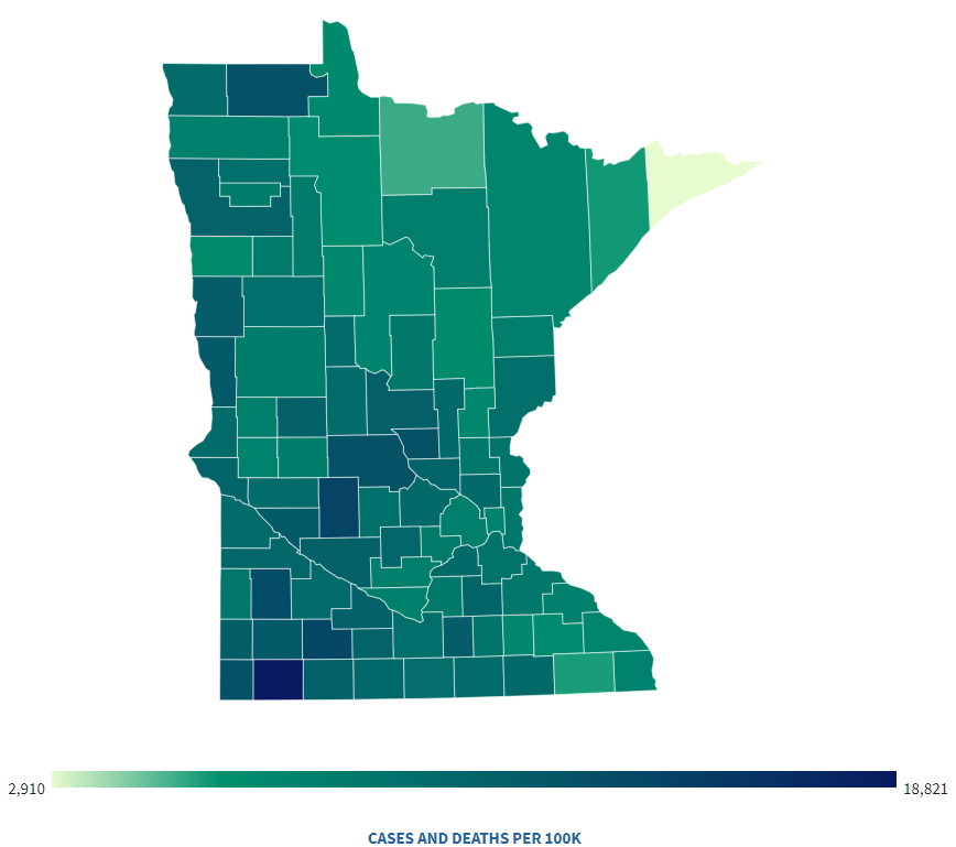
Figure 1: Infection map of Minnesota [31].

Through this formulation of $B$ and $W$, the weights in $W$ are proportional to the volume of travel between counties, and larger values of an entry $w_{ij}$ indicate a higher volume of travel between counties $i$ and $j$. We classify the weights into three categories, which are low, medium, and high travel flows, which correspond to the weight ranges $(0,0.01]$, $(0.01,0.1]$, and $(0.1,3]$, respectively. We set the adjacency parameter to $k=0.001$. This choice of $k$ is because over half of the entries in the weight matrix $W$ are much smaller than $k$, indicating that this choice of $k$ certainly fulfills our objective of protecting individuals. In fact, in more than half of the entries of $W$, it simultaneously protects all individuals whose travel is encoded in that entry. In our simulations, we generated $100$ private graphs for each $\epsilon\in[5,20]$ using Mechanism 1 on $G$.

We compute and plot the absolute differences $|\tilde{R}_{0}-R_{0}|$ and $\left|\frac{1}{\tilde{R}_{0}}-\frac{1}{R_{0}}\right|$ for each $\epsilon\in[5,20]$, which are shown in Figures 2 and 3, respectively. Recall from Remark 2 that higher values of the privacy parameter $\epsilon$ imply weaker privacy, and the simulation results confirm that weaker privacy guarantees result in smaller errors. For all values of $\epsilon\in[5,20]$, the empirical average of $|\tilde{R}_{0}-R_{0}|$ is small (between $0.27$ and $0.45$, incurring errors from $7.6\%$ to $12.7\%$ on average) compared to the true value $R_{0}=3.54$. Similarly, the empirical average of $\left|\frac{1}{\tilde{R}_{0}}-\frac{1}{R_{0}}\right|$ is from $0.019$ to $0.031$, incurring errors from $7.0\%$ to $11.2\%$. Additionally, both the values of $|\tilde{R}_{0}-R_{0}|$ and $\left|\frac{1}{\tilde{R}_{0}}-\frac{1}{R_{0}}\right|$ are concentrated around their empirical averages. These simulation results demonstrate that $\tilde{R}_{0}$ maintains enough accuracy under privacy to enable useful analyses alongside protecting information.

Figure 2: The value of $|\tilde{R}_{0}-R_{0}|$ as a function of the privacy parameter $\epsilon$ given $R_{0}=3.54$. Smaller values of $\epsilon$ correspond to stronger privacy.

Figure 3: The value of $\left|\frac{1}{\tilde{R}_{0}}-\frac{1}{R_{0}}\right|$ as a function of the privacy parameter $\epsilon$ given $\frac{1}{R_{0}}=0.283$. Smaller values of $\epsilon$ correspond to stronger privacy.

VI Conclusions

This paper presents an input perturbation mechanism that provides differential privacy to graph weights when computing the basic reproduction number of an epidemic spreading network. The proposed mechanism uses bounded noise and the corresponding privacy-accuracy tradeoffs are quantified. We also develop a concentration bound to evaluate privacy-accuracy tradeoffs in terms of the remaining susceptible population within a community when the proposed mechanism is applied to a networked SIS or SIR model. Future works include applications of the proposed privacy mechanism in the control of epidemic spreading.

We first state results that will be used later in proofs.

Definition 5 (Sub-Gaussian random variable[33]).

A random variable $X\in\mathbb{R}$ is sub-Gaussian with variance proxy $\sigma_{SG}$, written as $X\sim\text{subG}(\sigma_{SG}^{2})$, if $\mathbb{E}[X]=0$ and $\mathbb{E}[\exp(\eta X)]\leq\exp\left(\frac{\eta^{2}\sigma_{SG}^{2}}{2}\right)$, where $\mathbb{E}[\exp(\eta X)]$ is the moment generating function of random variable $X$. $\lozenge$

A truncated Gaussian random variable can be expressed as a sub-Gaussian random variable.

Lemma 1.

If $Y\sim\text{TrunG}(\mu,\sigma,l,u)$, then we have that ${Y-\mathbb{E}[Y]\sim\text{subG}(\sigma^{2})}$.

Proof of Lemma 1: The proof of Lemma 1 will use the following lemma.

Lemma 2.

[30, Chapter 3] If $Y\sim\text{TrunG}(\mu,\sigma,l,u)$, then

$$\mathbb{E}[Y]=\mu+\sigma\cdot\frac{\varphi\left(\alpha\right)-\varphi\left(\beta\right)}{\Phi\left(\beta\right)-\Phi\left(\alpha\right)},$$ (18)

$$\text{Var}[Y]=\sigma^{2}\left[1-\frac{\beta\varphi(\beta)-\alpha\varphi(\alpha)}{\Phi\left(\beta\right)-\Phi\left(\alpha\right)}-\left(\frac{\varphi\left(\alpha\right)-\varphi\left(\beta\right)}{\Phi\left(\beta\right)-\Phi\left(\alpha\right)}\right)^{2}\right],$$ (19)

$$\mathbb{E}[\exp(\eta X)]=\exp\left(\mu\eta+\frac{\sigma^{2}\eta^{2}}{2}\right)$$ (20)

$$\qquad\qquad\qquad\quad\qquad\cdot\left[\frac{\Phi\left(\beta-\sigma\eta\right)-\Phi\left(\alpha-\sigma\eta\right)}{\Phi\left(\beta\right)-\Phi\left(\alpha\right)}\right],$$ (21)

where $\alpha=\frac{l-\mu}{\sigma}$ and $\beta=\frac{u-\mu}{\sigma}$. $\blacksquare$

The proof then proceeds by extending the moment generating function of $Y$. By (21) we have

$$\mathbb{E}[\exp(\eta Y)]=\exp\left(\mu\eta+\frac{\sigma^{2}\eta^{2}}{2}+f(\eta)\right),$$ (22)

where $f(\eta)=\log\left(\frac{\Phi\left(\beta-\sigma\eta\right)-\Phi\left(\alpha-\sigma\eta\right)}{\Phi\left(\beta\right)-\Phi\left(\alpha\right)}\right)$. We now take the Taylor expansion of $f$ about $\eta=0$ to find

$$f(\eta)=f(0)+\left(\frac{\partial f(\eta)}{\partial\eta}\Bigr{|}_{\eta=0}\right)\eta+\frac{1}{2}\left(\frac{\partial^{2}f(\eta)}{\partial\eta^{2}}\Bigr{|}_{\eta=\delta}\right)\delta^{2},$$ (23)

where $\delta\in(0,\eta)$. We note that $f(0)=0$ and the first derivative evaluated at $\eta=0$ is

$$\frac{\partial f(\eta)}{\partial\eta}\Bigr{|}_{\eta=0} =\sigma\cdot\frac{\varphi(\alpha)-\varphi(\beta)}{\Phi(\beta)-\Phi(\alpha)}.$$ (24)

For all $\eta>0$, we have $\frac{\partial^{2}f(\eta)}{\partial\eta^{2}}\leq 0.$ Therefore,

$$f(\eta)\leq\sigma\eta\cdot\frac{\varphi(\alpha)-\varphi(\beta)}{\Phi(\beta)-\Phi(\alpha)}.$$ (25)

We then conclude by extending the moment generating function of $Y-E[Y]$ and plugging in (18) and (25) to find $\mathbb{E}[\exp(\eta(Y-\mathbb{E}[Y]))]=\exp(-\eta\mathbb{E}[Y])\mathbb{E}[\exp(\eta Y)]\leq\exp\left(\frac{\sigma^{2}\eta^{2}}{2}\right)$. $\blacksquare$

-A Proof of Theorem 1

Networked $SIS$ and $SIR$ models are special cases of the coupled system in [25, Eq. (2)-(4)], as described in [25, Fig. 1]. We leverage [25, Thm. 5] for the coupled system in [25, Eq. (2)-(4)] to study the networked $SIS$ and $SIR$ models in (6)-(8). In order to leverage [25, Thm. 5], we investigate if the system (6) -(8) satisfies  [25, Assump. 3 and 4], and the preconditions of the dynamics in [25, Eq. (2)-(4)].

We discuss networked $SIR$ models first. Networked compartmental models such as $SIR$ models are groups of polynomial ODEs over the compact set $[0,1]^{n}$. Hence, (4) are locally Lipschitz in states $s(t)$, $x(t)$, $r(t)$, which satisfies the condition that the system dynamics in  [25, Eq. (2)] must be locally Lipschitz in their states. Further, $I>0$ and $B>0$ in (8) guarantee that the nonlinear dynamics of $s(t)$ in (6) satisfy the definition of [25, Eq. (2)], where $M_{1}>0$ and $M_{2}>0$ in [25, Eq. (2)]. For networked $SIR$ models, the states of each community obey $s_{i}(t),x_{i}(t)\in[0,1]$ for all $i\in[n]$. Therefore, the LTI system with external input $u(t)$ that captures the infected states $x(t)$ in (8) is internally positive. In addition, $-\Gamma$ is a Hurwitz and Metzler matrix, since $-\Gamma$ is a negative definite diagonal matrix, where the $i^{th}$ diagonal entry is the recovery rate $\gamma_{i}$ of community $i$. By comparing [25, Eq. (3)] and (8), $I>0$ is a nonzero, nonnegative matrix. Therefore, the preconditions in [25, Eq. (2)], namely that $B>0$ and $C>0$, hold here.

Next, we check if (6)-(8) satisfy [25, Assump. 3 and 4]. The  [25, Assump. 3] considers $(x^{*},u^{*})$ such that $\dot{x}=0$ in (8), and such that for sufficiently small $\nu>0$, it holds that $u\neq u^{*}$ and $\|u-u^{*}\|<\nu$ imply $\dot{x}\neq 0$ at $x^{*}$ and $u$.

Consider (8). When $\dot{x}=0$, we have that $-\Gamma x^{*}+Iu^{*}=0$. For any $u$ such that $\|u-u^{*}\|<\nu$, where $\nu>0$ can be sufficiently small, we have that $-\Gamma x^{*}-Iu=0-\Gamma x^{*}-Iu=I(u^{*}-u)$. Note that we use the fact that (8) is a linear system. Since $I\neq 0$ and $\|u-u^{*}\|<\nu$, we have $\dot{x}=-\Gamma x^{*}+Iu\neq 0$. Thus, [25, Assump. 3] holds for (8).

As for [25, Assump. 4], we need to investigate the set of the initial conditions of interest $\mathcal{I}$. If $(s(0),x(0))\in\mathcal{I}$, $\lim_{t\rightarrow\infty}s(t)=s^{*}$ exists. Further, $\mathcal{I}$ must satisfy the condition that if $(s(0),x(0))\in\mathcal{I}$, we can always find a $\tau>0$ such that for any $x>0$, $(s^{*},\tau x)\in\mathcal{I}$.

Without considering the dynamics of $r(t)$, for networked $SIR$ models, $\lim_{t\rightarrow\infty}s(t)=s^{*}$ exists if $(s(0),x(0))\in[0,1]^{2n}$ [2]. Therefore, we assume $\mathcal{I}=[0,1]^{2n}$. Then we show that if $\mathcal{I}=[0,1]^{2n}$ satisfies [25, Assump. 4]. We consider two sets of initial conditions $\mathcal{I}_{1},\mathcal{I}_{2}\subset[0,1]^{2n}=\mathcal{I}$, where $\mathcal{I}_{1}\cap\mathcal{I}_{2}=\emptyset$ and $\mathcal{I}_{1}\cup\mathcal{I}_{2}=\mathcal{I}$. We define $\mathcal{I}_{1}=\{(s(0)=1,x(0)=0)\}$ that describes a trivial initial condition where no epidemic occurs, i.e., $\lim_{t\rightarrow\infty}s(t)=s^{*}=1$ and $x^{*}=0$. Under this condition, we cannot find a $\tau>0$ such that for any $x>0$, $(1,\tau x)\in\mathcal{I}_{1}$. Hence, although $\mathcal{I}_{1}\subset\mathcal{I}$, it does not satisfy  [25, Assump. 4]. Consider the set $\mathcal{I}_{2}=[0,1]^{2n}\backslash\mathcal{I}_{1}$. The set $\mathcal{I}_{2}$ describes the initial conditions where at least one community has nonzero infections. For networked $SIR$ models, an initial condition in $\mathcal{I}_{2}$ guarantees $s^{*}<1$ [4, 2]. For any $x>0$, we can always find a $\tau>0$ such that $s^{*}+\tau x<1$, since $s^{*}<1$. Hence, we can find a valid initial condition $(s^{*},\tau x)\in\mathcal{I}_{2}$. We prove that the non-trivial initial conditions in $\mathcal{I}_{2}$ for networked $SIR$ models always satisfy [25, Assump. 4]. Note that when we study networked $SIR$ models, we always consider initial conditions from $\mathcal{I}_{2}$.

Recall that we represent networked $SIR$ models as the coupled systems in (6)-(8). After proving that the networked $SIR$ dynamics captured by (6)-(8) meet [25, Assump. 3 and 4] and the predictions, we can implement  [25, Them. 1] to study disease-free equilibria of the networked $SIR$ models. Since the transmission network is undirected and connected, we can treat the underlying graph as being directed and strongly connected by replacing each undirected edge with two directed edges in the obvious way. Further, the transmission matrix $B$ is a symmetric irreducible matrix. The healing matrix $\Gamma$ is a positive definite diagonal matrix, resulting in $W=B\Gamma^{-1}$ being a Metzler and irreducible matrix. Through [25, Them. 1], at a disease-free equilibrium of the networked $SIR$ model, there must exist a community within the network whose susceptible proportion is given by

$$s^{*}_{i} \leq\frac{1}{\rho(-M_{2}CA^{-1}FM_{1})}=\frac{1}{\rho(-\Gamma^{-1}B)}=\frac{1}{R_{0}}.\vspace{-4ex}$$ (26)

This completes the proof for networked $SIR$ models.

For networked $SIS$ models, we show a straightforward conclusion. We know that $s^{*}=1$ and $x^{*}=0$ is the unique disease-free equilibrium for networked $SIS$ models [2, 4]. Further, networked $SIS$ models will reach the disease-free equilibrium if and only if $R_{0}\leq 1$ [2]. Hence, we have that for networked $SIS$ models at their disease-free equilibrium, $s^{*}_{i}=1\leq\frac{1}{R_{0}}$ for all $i\in[n]$. $\blacksquare$

-B Proof of Theorem 2

Let $\tilde{W}=W+P$, where the matrix $P$ encodes the differences between $\tilde{W}$ and $W$. Then we have the equalities $\tilde{R}_{0}-R_{0}=\rho(\tilde{W})-\rho(W)=\rho(W+P)-\rho(W)$. Since both $W$ and $P$ are symmetric, we apply [34, Theorem 8.4.11] to split $\rho(W+P)$ and then apply Weyl’s inequality [34, Fact 9.12.4] to find

$$|\rho(W+P)-\rho(W)|\leq||P||_{2}\leq||P||_{F},$$ (27)

where $||\cdot||_{2}$ is the $L_{2}$-norm of a matrix. Now we take the expectation on both sides of (27) and apply Jensen’s inequality to find

$$\mathbb{E}[|\tilde{R}_{0} -R_{0}|]\leq\mathbb{E}[||P||_{F}]$$ (28)

$$=\mathbb{E}\left[\sqrt{\sum_{i=1}^{n}\sum_{j=1}^{n}(p_{ij})^{2}}\right]\leq\sqrt{\mathbb{E}\left[\sum_{i=1}^{n}\sum_{j=1}^{n}(p_{ij})^{2}\right]}$$ (29)

$$=\sqrt{\sum_{i=1}^{n}\sum_{j=i+1}^{n}2\mathbb{E}\left[(p_{ij})^{2}\right]+\sum_{i=1}^{n}\mathbb{E}\left[(p_{ii})^{2}\right]},$$ (30)

where $p_{ij}$ is the $i^{th},j^{th}$ entry of $P$. Equation (30) holds because each $p_{ij}$ above the main diagonal is generated independently and the matrix $P$ is symmetric. We note that $p_{ij}\sim\text{TrunG}(0,\sigma,\underline{w}_{ij}-w_{ij},\bar{w}_{ij}-w_{ij})$. We apply the equality $\mathbb{E}[X^{2}]=(\mathbb{E}[X])^{2}+\text{Var}[X]$ for any random variable $X$ and $\mathbb{E}[p_{ij}]=\text{Var}[p_{ij}]=0$ if $p_{ij}=0$ to have

$$\vspace{-4ex}\quad(\mathbb{E}\left[p_{ij}\right])^{2}+\text{Var}[p_{ij}]\\ =\sigma^{2}\left(1-\frac{\beta_{ij}\varphi(\beta_{ij})-\alpha_{ij}\varphi(\alpha_{ij})}{\Phi(\beta_{ij})-\Phi(\alpha_{ij})}\right)\cdot\mathbf{1}_{\mathbb{R}_{>0}}(w_{ij}),$$ (31)

where $\mathbb{E}[p_{ij}]$ and $\text{Var}[p_{ij}]$ can be found by Lemma 2. Additionally, by (27) and $\text{Var}[X]\leq\mathbb{E}[X^{2}]$ for any $X$, we have

$$\text{Var}[|\tilde{R}_{0}-R_{0}|] \leq\mathbb{E}[||P||_{F}^{2}]\leq\mathbb{E}\left[\sum_{i=1}^{n}\sum_{j=1}^{n}(p_{ij})^{2}\right].$$ (32)

We conclude by applying (30) and (31). $\blacksquare$

-C Proof of Theorem 3

We introduce the following lemma for Theorem 3.

Lemma 3.

[35, Corollary 4.4.8] Let $H$ be an $n\times n$ random symmetric matrix whose entries $H_{ij}$ on and above the main diagonal are independent, mean zero, sub-Gaussian random variables with proxy $\sigma^{2}$. Then, for any $v>0$ we have $\mathbb{P}\big{[}||H||_{2}\geq t\big{]}\leq 4\exp\left(-\frac{v^{2}}{2\sigma^{2}}\right)$, where $t=\sqrt{2\sigma^{2}(4.4n+v^{2})}$. $\blacksquare$

For a private undirected graph $\tilde{G}=(V,E,\tilde{W})$, we write $\tilde{W}=W+M+A$, where $M=[m_{ij}]^{n\times n}$ is a deterministic symmetric matrix with $m_{ij}=\mathbb{E}[\tilde{w}_{ij}-w_{ij}]$. The matrix $A=[a_{ij}]^{n\times n}$ captures all the random parts with $a_{ij}\sim\text{TrunG}(-m_{ij},\sigma,\underline{w}_{ij}-w_{ij}-m_{ij},\bar{w}_{ij}-w_{ij}-m_{ij})$. Note that $\mathbb{E}[a_{ij}]=0$ for every $i,j\in[n]$. Applying Weyl’s inequality [34, Fact 9.12.4] to obtain the inequality $|\rho(\tilde{W})-\rho(W)|\leq||\tilde{W}-W||_{2}\leq||M||_{F}+||A||_{2}$. Based on (18),

$$||M||_{F} =\sqrt{\sum_{i=1}^{n}\sum_{j=1}^{n}m_{ij}^{2}}=\sqrt{\sum_{i=1}^{n}\sum_{j=1}^{n}(\mathbb{E}[\tilde{w}_{ij}-w_{ij}])^{2}},$$ (33)

where $(\mathbb{E}[\tilde{w}_{ij}-w_{ij}])^{2}$ can be found using (18). Since the matrix $A$ is symmetric, by Lemma 3 we have

$$\mathbb{P}\Big{[}|\rho(\tilde{W})-\rho(W)|>t+||M||_{F}\Big{]}\\ \quad\leq\mathbb{P}\Big{[}||A||_{2}+||M||_{F}>t+||M||_{F}\Big{]}\leq 4\exp\left(-\frac{v^{2}}{2\sigma^{2}}\right).$$ (34)

We conclude the proof by rearranging the terms above. $\blacksquare$

References

- [1] F. Brauer, “Compartmental models in epidemiology,” Math. Epi., pp. 19–79, 2008.
- [2] P. E. Paré, C. L. Beck, and T. Başar, “Modeling, estimation, and analysis of epidemics over networks: An overview,” Annual Reviews in Control, vol. 50, pp. 345–360, 2020.
- [3] B. She, H. C. Leung, S. Sundaram, and P. E. Paré, “Peak infection time for a networked SIR epidemic with opinion dynamics,” in In Proc. 60th IEEE Conf. on Dec. and Contr. IEEE, 2021, pp. 2104–2109.
- [4] W. Mei, S. Mohagheghi, S. Zampieri, and F. Bullo, “On the dynamics of deterministic epidemic propagation over networks,” Ann. Rev. in Cont., vol. 44, pp. 116–128, 2017.
- [5] D. Brockmann and D. Helbing, “The hidden geometry of complex, network-driven contagion phenomena,” Science, vol. 342, no. 6164, pp. 1337–1342, 2013.
- [6] Y. Bengio, R. Janda, Y. W. Yu, D. Ippolito, M. Jarvie, D. Pilat, B. Struck, S. Krastev, and A. Sharma, “The need for privacy with public digital contact tracing during the COVID-19 pandemic,” The Lancet Digital Health, vol. 2, no. 7, pp. e342–e344, 2020.
- [7] P. L. Delamater, E. J. Street, T. F. Leslie, Y. T. Yang, and K. H. Jacobsen, “Complexity of the basic reproduction number (),” Emerging Infectious Diseases, vol. 25, no. 1, p. 1, 2019.
- [8] J. K. Aronson, J. Brassey, and K. R. Mahtani, “When will it be over?”: An introduction to viral reproduction numbers, and ,” The Centre for Evidence-Based Medicine, vol. 14, 2020.
- [9] J. Imola, T. Murakami, and K. Chaudhuri, “Locally differentially private analysis of graph statistics,” in Proc. 30th USENIX security symposium (USENIX Security 21), 2021, pp. 983–1000.
- [10] V. Karwa, S. Raskhodnikova, A. Smith, and G. Yaroslavtsev, “Private analysis of graph structure,” ACM Trans. Database Syst., vol. 39, no. 3, oct 2014.
- [11] W.-Y. Day, N. Li, and M. Lyu, “Publishing graph degree distribution with node differential privacy,” in Proc. 2016 Int. Conf. on Mana of Data, ser. SIGMOD ’16. New York, NY, USA: Association for Computing Machinery, 2016, p. 123–138.
- [12] S. Zhang, W. Ni, and N. Fu, “Differentially private graph publishing with degree distribution preservation,” Computers & Security, vol. 106, p. 102285, 2021.
- [13] B. Chen, C. Hawkins, K. Yazdani, and M. Hale, “Edge differential privacy for algebraic connectivity of graphs,” in Proc. 60th IEEE Conf. on Dec. and Cont. (CDC). IEEE, 2021, pp. 2764–2769.
- [14] “Why the Census Bureau chose differential privacy,” U.S. Census Bureau, 2023.
- [15] A. Sealfon, “Shortest paths and distances with differential privacy,” ser. PODS ’16. New York, NY, USA: Association for Computing Machinery, 2016, p. 29–41.
- [16] R. Pinot, A. Morvan, F. Yger, C. Gouy-Pailler, and J. Atif, “Graph-based Clustering under Differential Privacy,” in Proc. Conf. on Uncer. in Art. Int. (UAI 2018), Monterey, California, United States, Aug. 2018, pp. 329–338.
- [17] C. Dwork, A. Roth et al., “The algorithmic foundations of differential privacy,” Foundations and Trends® in Theoretical Computer Science, vol. 9, no. 3–4, pp. 211–407, 2014.
- [18] B. Chen and M. Hale, “The bounded Gaussian mechanism for differential privacy,” arXiv preprint arXiv:2211.17230, 2022.
- [19] C. Hawkins, B. Chen, K. Yazdani, and M. Hale, “Node and edge differential privacy for graph Laplacian spectra: Mechanisms and scaling laws,” arXiv preprint arXiv:2211.15366, 2022.
- [20] M. Hay, C. Li, G. Miklau, and D. Jensen, “Accurate estimation of the degree distribution of private networks,” in Proc. 2009 Ninth IEEE Int. Conf. on Data Mining, 2009, pp. 169–178.
- [21] J. Blocki, A. Blum, A. Datta, and O. Sheffet, “Differentially private data analysis of social networks via restricted sensitivity,” arXiv preprint arXiv:1208.4586, 2013.
- [22] S. P. Kasiviswanathan, K. Nissim, S. Raskhodnikova, and A. Smith, “Analyzing graphs with node differential privacy,” in Theory of Cryptography, A. Sahai, Ed. Berlin, Heidelberg: Springer Berlin Heidelberg, 2013, pp. 457–476.
- [23] Y. Wang, X. Wu, and L. Wu, “Differential privacy preserving spectral graph analysis,” in Proc. Advan.s in Kno. Disc. and Data Min. Berlin, Heidelberg: Springer Berlin Heidelberg, 2013, pp. 329–340.
- [24] T. Chanyaswad, A. Dytso, H. V. Poor, and P. Mittal, “Proc. MVG mechan.: Diff. priv. under matrix-valued query,” in Proceedings of the 2018 ACM SIGSAC Conf. on Comp. and Commu. Secu., ser. CCS ’18. New York, NY, USA: Assoc. for Comp. Mach., 2018, p. 230–246.
- [25] S. Zhen Khong and L. Su, “Steady-state analysis of networked epidemic models,” arXiv e-prints, pp. arXiv–2305, 2023.
- [26] M. Jagielski, J. Ullman, and A. Oprea, “Auditing differentially private machine learning: How private is private SGD?” arXiv preprint arXiv:2006.07709, 2020.
- [27] M. Nasr, S. Song, A. Thakurta, N. Papernot, and N. Carlini, “Adversary instantiation: Lower bounds for differentially private machine learning,” arXiv preprint arXiv:2101.04535, 2021.
- [28] C. Song and V. Shmatikov, “Auditing data provenance in text-generation models,” arXiv preprint arXiv:1811.00513, 2019.
- [29] B. Balle, G. Cherubin, and J. Hayes, “Reconstructing training data with informed adversaries,” arXiv preprint arXiv:2201.04845, 2022.
- [30] J. Burkardt, “The truncated normal distribution,” Department of Scientific Computing Website, Florida State University, vol. 1, p. 35, 2014.
- [31] “Minnesota coronavirus cases and deaths,” 2023. [Online]. Available: https://doi.org/10.1145/237814.237880
- [32] B. A. Butler, R. Stern, and P. E. Paré, “Analysis and applications of population flows in a networked SEIRS epidemic process,” ArXiv, 2023, arXiv:2309.11588 [math.OC].
- [33] V. V. Buldygin and Y. V. Kozachenko, “Sub-gaussian random variables,” vol. 32, no. 6, pp. 483–489.
- [34] D. Bernstein, Matrix Mathematics: Theory, Facts, and Formulas (Second Edition), ser. Princeton reference. Princeton University Press, 2009.
- [35] R. Vershynin, High-Dimensional Probability: An Introduction with Applications in Data Science, ser. Cambridge Series in Statistical and Probabilistic Mathematics. Cambridge University Press, 2018.