Information Flow in Self-Supervised Learning

Abstract

In this paper, we provide a comprehensive toolbox for understanding and enhancing self-supervised learning (SSL) methods through the lens of matrix information theory. Specifically, by leveraging the principles of matrix mutual information and joint entropy, we offer a unified analysis for both contrastive and feature decorrelation based methods. Furthermore, we propose the matrix variational masked auto-encoder (M-MAE) method, grounded in matrix information theory, as an enhancement to masked image modeling. The empirical evaluations underscore the effectiveness of M-MAE compared with the state-of-the-art methods, including a $3.9\%$ improvement in linear probing ViT-Base, and a $1\%$ improvement in fine-tuning ViT-Large, both on ImageNet.

1 Introduction

Self-supervised learning (SSL) has demonstrated remarkable advancements across various tasks, including image classification and segmentation, often surpassing the performance of supervised learning approaches  [10, 9, 32, 61, 5]. Broadly, SSL methods can be categorized into three types: contrastive learning, feature decorrelation based learning, and masked image modeling.

One prominent approach in contrastive self-supervised learning is SimCLR [10], which employs the InfoNCE loss [35] to facilitate the learning process. Interestingly, Oord et al. [35] show that InfoNCE loss can serve as a surrogate loss for the mutual information between two augmented views. Unlike contrastive learning which needs to include large amounts of negative samples to “contrast”, another line of work usually operates without explicitly contrasting with negative samples which we call feature decorrelation based learning. Recently, there has been a growing interest in developing feature decorrelation based SSL methods, e.g., BYOL [19], SimSiam [11], Barlow Twins [61], VICReg [5], etc. These methods have garnered attention from researchers seeking to explore alternative avenues for SSL beyond contrastive approaches.

On a different note, the masked autoencoder (MAE) [23] introduces a different way to tackle self-supervised learning. Unlike contrastive and feature decorrelation based methods that learn useful representations by exploiting the invariance between augmented views, MAE employs a masking strategy to have the model deduce the masked patches from visible patches. Therefore, the representation of MAE carries valuable information for downstream tasks.

At first glance, these three types of self-supervised learning methods may seem distinct, but researchers have made progress in understanding their connections. Garrido et al. [16] establish a duality between contrastive and feature decorrelation based methods, shedding light on their fundamental connections and complementarity. Additionally, Balestriero & LeCun [4] unveil the links between popular feature decorrelation based SSL methods and dimension reduction methods commonly employed in traditional unsupervised learning. These findings contribute to our understanding of the theoretical underpinnings and potential applications of feature decorrelation based SSL techniques. However, compared to connections between contrastive and feature decorrelation based methods, the relationship between MAE and contrastive or feature decorrelation based methods remains largely unknown. To the best of our knowledge, [62] is the only paper that relates MAE to the alignment term in contrastive learning.

Though progress has been made in understanding the existing self-supervised learning methods, the tools used in the literature are diverse. As contrastive and feature decorrelation based learning usually use two augmented views of the same image, one prominent approach is analyzing the mutual information between two views [35, 41, 40]. A unified toolbox to understand and improve self-supervised methods is needed. Recently, [2, 42] have considered generalizing the traditional information-theoretic quantities to the matrix regime. Interestingly, we find these quantities can be powerful tools in understanding and improving existing self-supervised methods regardless of whether they are contrastive, feature decorrelation-based, or masking-based [23].

Taking the matrix information theoretic perspective, we analyze some prominent contrastive and feature decorrelation based losses and prove that both Barlow Twins and spectral contrastive learning [21] are maximizing mutual information and joint entropy. These claims are crucial for analyzing contrastive and feature decorrelation based methods, offering a cohesive and elegant understanding. More interestingly, the same analytical framework extends to MAE as well, wherein the concepts of mutual information and joint entropy gracefully degenerate to entropy. Propelled by this observation, we augment the MAE loss with matrix entropy, giving rise to our new method, Matrix variational Masked Auto-Encoder (M-MAE). Empirically, M-MAE stands out with commendable performance. Specifically, it has achieved a $3.9\%$ improvement in linear probing ViT-Base, and a $1\%$ improvement in fine-tuning ViT-Large, both on ImageNet. This empirical result not only underscores the efficacy of M-MAE but also accentuates the potential of matrix information theory in ushering advancements in self-supervised learning paradigms.

In summary, our contributions can be listed as follows:

• We use the matrix information-theoretic tools to understand existing contrastive and feature decorrelation based self-supervised methods.

• We introduce a novel method, M-MAE, which is rooted in matrix information theory, enhancing the capabilities of standard masked image modeling.

• Our proposed M-MAE has demonstrated remarkable empirical performance, showcasing a notable improvement in self-supervised learning benchmarks.

2 Background

2.1 Matrix Information-theoretic Quantities

In this section, we shall briefly summarize the matrix information-theoretic quantities that we shall use in this paper. We shall first provide the definition of (matrix) entropy as follows:

Definition 1 (Matrix-based $\alpha$-order (Rényi) entropy [42]).

Suppose matrix $\mathbf{K}_{1}\in\mathbb{R}^{n\times n}$ which $\mathbf{K}_{1}(i,i)=1$ for every $i=1,\cdots,n$. $\alpha$ is a positive real number. The $\alpha$-order (Rényi) entropy for matrix $\mathbf{K}_{1}$ is defined as follows:

$$\operatorname{H}_{\alpha}\left(\mathbf{K}_{1}\right)=\frac{1}{1-\alpha}\log\left[\operatorname{tr}\left(\left(\frac{1}{n}\mathbf{K}_{1}\right)^{\alpha}\right)\right],$$

where $\mathbf{K}^{\alpha}_{1}$ is the matrix power.

The case of $\alpha=1$ recovers the von Neumann (matrix) entropy, i.e.

$$\operatorname{H}_{1}\left(\mathbf{K}_{1}\right)=-\operatorname{tr}\left(\frac{1}{n}\mathbf{K}_{1}\log\frac{1}{n}\mathbf{K}_{1}\right).$$

Using the definition of matrix entropy, we can define matrix mutual information and joint entropy as follows.

Definition 2 (Matrix-based mutual information).

Suppose matrix $\mathbf{K}_{1},\mathbf{K}_{2}\in\mathbb{R}^{n\times n}$ which $\mathbf{K}_{1}(i,i)=\mathbf{K}_{2}(i,i)=1$ for every $i=1,\cdots,n$. $\alpha$ is a positive real number. The $\alpha$-order (Rényi) mutual information for matrix $\mathbf{K}_{1}$ and $\mathbf{K}_{2}$ is defined as follows:

$$\operatorname{I}_{\alpha}(\mathbf{K}_{1};\mathbf{K}_{2})=\operatorname{H}_{\alpha}(\mathbf{K}_{1})+\operatorname{H}_{\alpha}(\mathbf{K}_{2})-\operatorname{H}_{\alpha}(\mathbf{K}_{1}\odot\mathbf{K}_{2}).$$

Definition 3 (Matrix-based joint entropy).

Suppose matrix $\mathbf{K}_{1},\mathbf{K}_{2}\in\mathbb{R}^{n\times n}$ which $\mathbf{K}_{1}(i,i)=\mathbf{K}_{2}(i,i)=1$ for every $i=1,\cdots,n$. $\alpha$ is a positive real number. The $\alpha$-order (Rényi) joint-entropy for matrix $\mathbf{K}_{1}$ and $\mathbf{K}_{2}$ is defined as follows:

$$\operatorname{H}_{\alpha}(\mathbf{K}_{1},\mathbf{K}_{2})=\mathbf{H}_{\alpha}(\mathbf{K}_{1}\odot\mathbf{K}_{2}),$$

where $\odot$ is the (matrix) Hadamard product.

Another important quantity is the matrix KL divergence defined as follows.

Definition 4 (Matrix KL divergence [2]).

Suppose matrix $\mathbf{K}_{1},\mathbf{K}_{2}\in\mathbb{R}^{n\times n}$ which $\mathbf{K}_{1}(i,i)=\mathbf{K}_{2}(i,i)=1$ for every $i=1,\cdots,n$. The Kullback-Leibler (KL) divergence between these two matrices $\mathbf{K}_{1}$ and $\mathbf{K}_{2}$ is defined as

$$\operatorname{KL}\left(\mathbf{K}_{1}\mid\mid\mathbf{K}_{2}\right)=\operatorname{tr}\left[\mathbf{K}_{1}\left(\log\mathbf{K}_{1}-\log\mathbf{K}_{2}\right)\right].$$

2.2 Canonical Self-Supervised Learning Losses

We shall recap some canonical losses used in self-supervised learning. As we roughly characterize self-supervised learning into contrastive learning, feature decorrelation based learning, and masked image modeling. We shall introduce the canonical losses used in these areas sequentially.

In contrastive and feature decorrelation based learning, people usually adopt the Siamese architecture, namely using two parameterized networks: the online network ${f}_{\theta}$ and the target network ${f}_{\phi}$. To create different perspectives of a batch of $B$ data points $\{\mathbf{x}_{i}\}^{B}_{i=1}$, we randomly select an augmentation $\mathcal{T}$ from a predefined set $\tau$ and use it to transform each data point, resulting in new representations $\mathbf{z}^{(1)}_{i}={f}_{\theta}(\mathcal{T}(\mathbf{x}_{i}))\in\mathbb{R}^{d}$ and $\mathbf{z}^{(2)}_{i}={f}_{\phi}(\mathbf{x}_{i})\in\mathbb{R}^{d}$ generated by the online and target networks, respectively. We then combine these representations into matrices $\mathbf{Z}_{1}=[\mathbf{z}^{(1)}_{1},\ldots,\mathbf{z}^{(1)}_{B}]$ and $\mathbf{Z}_{2}=[\mathbf{z}^{(2)}_{1},\ldots,\mathbf{z}^{(2)}_{B}]$. In masked image modeling, people usually adopt only one branch and do not use Siamese architecture.

The idea of contrastive learning is to make the representation of similar objects align and dissimilar objects apart. One of the widely adopted losses in contrastive learning is InfoNCE loss [10], which is defined as follows:

$$\mathcal{L}_{\text{InfoNCE}}=-\frac{1}{2}(\sum^{B}_{i=1}\log\frac{\exp{((\mathbf{z}^{(1)}_{i})^{\top}\mathbf{z}^{(2)}_{i})}}{\sum^{B}_{j=1}\exp{((\mathbf{z}^{(1)}_{i})^{\top}\mathbf{z}^{(2)}_{j}})}+\sum^{B}_{i=1}\log\frac{\exp{((\mathbf{z}^{(2)}_{i})^{\top}\mathbf{z}^{(1)}_{i})}}{\sum^{B}_{j=1}\exp{((\mathbf{z}^{(2)}_{i})^{\top}\mathbf{z}^{(1)}_{j}})}).$$ (1)

As the InfoNCE loss may be difficult to analyze theoretically, HaoChen et al. [21] then propose spectral contrastive loss as a good surrogate for InfoNCE. The loss is defined as follows:

$$\sum^{B}_{i=1}\mid\mid\mathbf{z}^{(1)}_{i}-\mathbf{z}^{(2)}_{i}\mid\mid^{2}_{2}+\lambda\sum_{i\neq j}((\mathbf{z}^{(1)}_{i})^{\top}\mathbf{z}^{(2)}_{j})^{2},$$ (2)

where $\lambda$ is a hyperparameter.

The idea of feature decorrelation based learning is to learn useful representation by decorrelating features and do not explicit distinguishes negative samples. Some notable losses involve VICReg [5], Barlow Twins [61]. The Barlow Twins loss is given as follows:

$$\sum^{B}_{i=1}\left(1-\mathcal{C}_{ii}\right)^{2}+\lambda\sum^{B}_{i=1}\sum_{j\neq i}\mathcal{C}_{ij}{}^{2},$$ (3)

where $\lambda$ is a hyperparameter and $\mathcal{C}_{ij}$ is the cross-correlation coefficient.

The idea of masked image modeling is to learn useful representations by generating the representation from partially visible patches and predicting the rest of the image from the representation, thus useful information in the image remains in the representation. We shall briefly introduce MAE [23] as an example. Given a batch of images $\{\mathbf{x}_{i}\}^{B}_{i=1}$, we shall first partition each of the images into $n$ disjoint patches $\mathbf{x}_{i}=\mathbf{x}_{i}(j)$ ($1\leq j\leq n$). Then $B$ random mask vectors $\mathbf{m}_{i}\in\{0,1\}^{n}$ will be generated, and denote the two images generated by these masks as

$$\mathbf{x}^{(1)}_{i}=\mathbf{x}_{i}\odot\mathbf{m}_{i}\quad\text{and}\quad\mathbf{x}^{(2)}_{i}=\mathbf{x}_{i}\odot(1-\mathbf{m}_{i}).$$ (4)

The model consists of two modules: an encoder $f$ and a decoder $g$. The encoder transform each view $\mathbf{x}^{(1)}_{i}$ into a representation $\mathbf{z}_{i}=f(\mathbf{x}^{(1)}_{i})$. The loss function is $\sum^{B}_{i=1}\mid\mid g(\mathbf{z}_{i})-\mathbf{x}^{(2)}\mid\mid_{2}^{2}$. We also denote the representations in a batch as $\mathbf{Z}=[\mathbf{z}_{1},\cdots,\mathbf{z}_{B}]$.

The goal of this paper is to use matrix information maximization viewpoint to understand the seemingly different losses in contrastive and Feature Decorrelation based methods. We would like also to use matrix information-theoretic tools to improve MAE. We only analyze $3$ popular losses: spectral contrastive, Barlow Twins and MAE.

3 Applying Matrix Information Theory to Contrastive and Feature Decorrelation Based Methods

As we have discussed in the preliminary session, in contrastive and feature decorrelation based methods, a common practice is to use two branches (Siamese architecture) namely an online network and a target network to learn useful representations. However, the relationship of the two branches during the training process is mysterious. In this section, we shall use matrix information quantities to unveil the complicated relationship in Siamese architectures.

3.1 Measuring the mutual information

One interesting derivation in [35] is that it can be shown that

$$\mathcal{L}_{\text{InfoNCE}}\geq-\operatorname{I}(\mathbf{Z}^{(1)};\mathbf{Z}^{(2)})+\log B,$$ (5)

where $\mathbf{Z}^{(i)}$ denotes the sampled distribution of the representation.

Though InfoNCE loss is a promising surrogate for estimating the mutual information between the two branches in self-supervised learning. [43] doubt its effectiveness when facing high-dimensional inputs, where the mutual information may be larger than $\log B$, making the bound vacuous. Then a natural question arises: Can we calculate the mutual information exactly? Unfortunately, it is hard to calculate the mutual information reliably and effectively. Thus we may change our strategy by using the matrix mutual information instead.

As the matrix mutual information has an exact and easy-to-calculate expression, one question remains: How to choose the matrices used in the (matrix) mutual information? We find the (batch normalized) sample covariance matrix serves as a good candidate. The reason is that by using batch normalization, the empirical covariance matrix naturally satisfies the requirements that: All the diagonals equal to $1$, the matrix is positive semi-definite and it is easy to estimate from data samples.

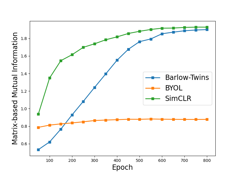
Figure 1: Visualization of matrix-based mutual information on CIFAR10 for Barlow-Twins, BYOL and SimCLR.

One vital problem with the bound Eqn. (5) is that it only provides an inequality, and thus doesn’t directly show the exact equivalence of contrastive learning and mutual information maximization. In the following, we will show that two pivotal self-supervised learning methods are exactly maximizing the mutual information.

We shall first present a proposition that bounds the (matrix) mutual information.

Proposition 1.

Suppose $\mathbf{K}_{1}$ and $\mathbf{K}_{2}$ are $d\times d$ positive semi-definite matrices with the constraint that each of its diagonals is $1$. Then $\operatorname{I}_{\alpha}(\mathbf{K}_{1};\mathbf{K}_{2})\leq\log d$.

One thing interesting in matrix information theory that distinguishes it from traditional information theory is that it can not only deal with samples from batches but also can exploit the relationship among batches, which we will informally call batch-dimension duality. Specifically, the sample covariance matrix can be expressed as $\mathbf{Z}\mathbf{Z}^{\top}\in\mathbb{R}^{d\times d}$ and the batch-sample Gram matrix can be expressed as $\mathbf{Z}^{\top}\mathbf{Z}\in\mathbb{R}^{B\times B}$. The closeness of these two matrices makes us call $B$ and $d$ has duality.

Notably, spectral contrastive loss [21] is a good surrogate loss for InfoNCE loss and calculates the loss involving the batch Gram matrix. Another famous loss used in feature decorrelation based methods is the Barlow Twins [61], which involves the batch-normalized sample covariance matrix. As we have discussed earlier, these two losses can be seen as a natural duality pair. In the following, we shall prove that these two losses exactly maximize the (matrix) mutual information by showing that these losses meet the bound in proposition 1.

Theorem 1.

Barlow twins and spectral contrastive learning seek the maximal mutual information.

Proof.

Please refer to Appendix A. ∎

We shall then plot the mutual information of covariance matrices between branches in Figure 1 by taking $\alpha=1$. We can find out that the mutual information increases during training, which is expected by Theorem 1. More interestingly, the mutual information of SimCLR and Barlow Twins meet at the end of training, strongly emphasizing the duality of these algorithms.

3.2 Measuring the (joint) entropy

After discussing the application of matrix mutual information in self-supervised learning. We wonder how the entropy evolves during the process.

Denote $\mathbf{K}_{1}=\mathbf{Z}_{1}\mathbf{Z}_{1}^{\top}$ and $\mathbf{K}_{2}=\mathbf{Z}_{2}\mathbf{Z}_{2}^{\top}$ for the online network and target network respectively. We can show that the matrix joint entropy can indeed reflect the dimensions of representations in Siamese architectures.

Proposition 2.

The joint entropy lower bounds the representation rank in two branches by having the inequality as follows:

$$\operatorname{H}_{1}(\mathbf{K}_{1},\mathbf{K}_{2})\leq\log(\operatorname{rank}(\mathbf{K}_{1}\odot\mathbf{K}_{2}))\leq\log\operatorname{rank}(\mathbf{K}_{1})+\log\operatorname{rank}(\mathbf{K}_{2}).$$ (6)

$$\max\{\operatorname{H}_{\alpha}(\mathbf{K}_{1}),\operatorname{H}_{\alpha}(\mathbf{K}_{2})\}\leq\operatorname{H}_{\alpha}(\mathbf{K}_{1},\mathbf{K}_{2})\leq\operatorname{H}_{\alpha}(\mathbf{K}_{1})+\operatorname{H}_{\alpha}(\mathbf{K}_{2}).$$ (7)

This proposition shows that the bigger the joint entropy between the two branches is, the less likely that the representation collapse. We shall also introduce another surrogate for entropy estimation which is closely related to matrix entropy:

Definition 5.

Suppose $B$ samples $\mathbf{Z}=[\mathbf{z}_{1},\mathbf{z}_{2},\cdots,\mathbf{z}_{B}]\in\mathbb{R}^{d\times B}$ are i.i.d. samples from a distribution $p(z)$. Then the total coding rate (TCR) [60] of $p(z)$ is defined as follows:

$$\text{TCR}_{\mu}(\mathbf{Z})=\log\operatorname{det}(\mu\mathbf{I}_{d}+\mathbf{Z}\mathbf{Z}^{\top}),$$ (8)

where $\mu$ is a non-negative hyperparameter.

For notation simplicity, we shall also write $\text{TCR}_{\mu}(\mathbf{Z})$ as $\text{TCR}_{\mu}(\mathbf{Z}\mathbf{Z}^{\top})$. We shall then show the close relationship between TCR and matrix entropy in the following theorem through the lens of matrix KL divergence. The key is utilizing the asymmetries of the matrix KL divergence.

Proposition 3.

Suppose $\mathbf{K}$ is a $d\times d$ matrix with the constraint that each of its diagonals is $1$. Then the following equalities holds:

$$\operatorname{H}_{1}(\mathbf{K})=\log d-\frac{1}{d}\operatorname{KL}(\mathbf{K},\mathbf{I}_{d}),\operatorname{and}\operatorname{TCR}_{\mu}(\mathbf{K})=d\log(1+\mu)-\operatorname{KL}(\mathbf{I}_{d},\frac{1}{1+\mu}(\mu\mathbf{I}_{d}+\mathbf{K})).$$ (9)

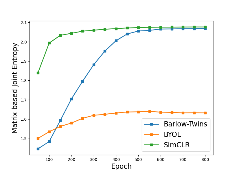
Figure 2: Visualization of matrix-based joint entropy on CIFAR10 for Barlow-Twins, BYOL and SimCLR.

As TCR can be treated as a good surrogate for entropy, we can obtain the following bound.

Proposition 4.

The (joint) total coding rate upperbounds the rate in two branches by having the inequality as follows:

$$\operatorname{TCR}_{\mu^{2}+2\mu}(\mathbf{K}_{1}\odot\mathbf{K}_{2})\geq\operatorname{TCR}_{\mu}(\mathbf{K}_{1})+\operatorname{TCR}_{\mu}(\mathbf{K}_{2}).$$ (10)

Combining Propositions 2, 3 and 4, it is clear that the bigger the entropy is for each branch the bigger the joint entropy. Thus by combining the conclusion from the above two theorems, it is evident that the joint entropy strongly reflects the extent of collapse during training.

What about the joint entropy when $\alpha=1$ behaves empirically? We shall then plot the joint entropy of covariance matrices between branches in Figure 2. We can find out that the joint entropy increases during training. More interestingly, the joint entropy of SimCLR and Barlow Twins meet at the end of training, strongly reflects a duality of these algorithms. Notably, we can also show that spectral contrastive and Barlow Twins maximize exactly the joint entropy between branches during training.

We shall first present a proposition that finds the optimal point of entropy.

Proposition 5.

$$\mathbf{I}_{d}=\operatorname*{arg\,max}\operatorname{H}_{\alpha}(\mathbf{K}),\operatorname{and}\mathbf{I}_{d}=\operatorname*{arg\,max}\operatorname{TCR}_{\mu}(\mathbf{K}),$$ (11)

where the maximization is over $d\times d$ positive semi-definite matrices with the constraint that each of its diagonals is $1$.

Proof.

The proof directly follows from proposition 3 and definition of entropy. ∎

Then we can show that spectral contrastive loss and Barlow twins loss can be seen as maximizing the joint entropy between branches.

Theorem 2.

Barlow twins and spectral contrastive learning seek the maximal (joint) entropy.

Proof.

Please refer to Appendix A. ∎

4 Applying Matrix Information Theory to Masked Image Modeling

As contrastive and feature decorrelation based methods usually surpass MAE by a large margin on linear probing. One may wonder if can we apply this matrix information theory to improve MAE. From a traditional information-theoretic point of view, when the two branches merge into one branch the mutual information $\operatorname{I}(\mathbf{X};\mathbf{X})$ and the joint entropy $\operatorname{H}(\mathbf{X},\mathbf{X})$ both equal to the Shannon entropy $\operatorname{H}(\mathbf{X})$. Thus we would like to use the matrix entropy in MAE training. Moreover, matrix entropy can be shown to be very close to a quantity called effective rank. And [62, 17] show that the effective rank is a critical quantity for better representation. The definition of effective rank is formally stated in Definition 6 and it is easy to show when the matrix is positive semi-definite and has all its diagonal being $1$ the effective rank is the exponential of the matrix entropy.

Definition 6 (Effective Rank [38]).

For a non-all-zero matrix $\mathbf{A}\in\mathbb{C}^{n\times n}$, the effective rank, denoted as $\operatorname{erank}(\mathbf{A})$, is defined as

$$\operatorname{erank}(\mathbf{A})\triangleq\exp{(\operatorname{H}\left(p_{1},p_{2},\ldots,p_{n}\right))},$$ (12)

where $p_{i}=\frac{\sigma_{i}}{\sum_{k=1}^{n}\sigma_{k}}$, $\{\sigma_{i}\mid i=1,\cdots,n\}$ represents the singular values of $\mathbf{A}$, and $\operatorname{H}$ denotes the Shannon entropy.

Thus it is natural to add the matrix entropy to the MAE loss to give a new self-supervised learning method. As the numerical instability of calculating matrix entropy is larger than its proxy TCR, we shall use TCR loss instead. One may wonder if we can link this new loss to other traditional unsupervised learning methods to give a better understanding. We answer this in the affirmative by linking this to the VAE approaches.

Recall the loss for traditional variational auto-encoder which is given as follows.

$$\mathcal{L}_{\text{VAE}}=\mathbb{E}_{\mathbf{x}\sim\tilde{p}(\mathbf{x})}[-\log q(\mathbf{x}\mid\mathbf{z})+\operatorname{KL}(p(\mathbf{z}\mid\mathbf{x})\|q(\mathbf{z}))],\quad\mathbf{z}\sim p(\mathbf{z}\mid\mathbf{x}).$$

The loss contains two terms, the first term $-\log q(\mathbf{x}\mid\mathbf{z})$ is a reconstruction loss that measures the decoding accuracy. The second term is a discriminative term, which measures the divergence of the encoder distribution $p(\mathbf{z}\mid\mathbf{x})$ with the latent distribution $q(\mathbf{z})$.

In the context of masked image modeling, we usually use MSE loss in place of the log-likelihood. For any input image $\mathbf{x}$, the process of randomly generating a masked vector $m$ and obtaining $\mathbf{z}=f(\mathbf{x}\odot\mathbf{m})$ can be seen as modeling the generating process of $\mathbf{z}\mid\mathbf{x}$. The decoding process $\mathbf{x}\mid\mathbf{z}$ can be modeled by concatenating $g(\mathbf{z})$ and $\mathbf{x}\odot\mathbf{m}$ by the (random) position induced by $m$. Thus the reconstruction loss will be $\mid\mid\text{concat}(g(\mathbf{z}),\mathbf{x}\odot\mathbf{m})-\mathbf{x}\mid\mid^{2}_{2}=\mid\mid g(\mathbf{z})-\mathbf{x}\odot(1-\mathbf{m})\mid\mid^{2}_{2}$. For a batch of images $\{\mathbf{x}_{i}\}^{B}_{i=1}$, this exactly recovers the MAE loss.

Recall that we assume each representation $z_{i}$ is $l_{2}$ normalized. If we take the latent distribution of ${Z}$ as the uniform distribution on the unit hyper-sphere $S^{d-1}$, we shall get the following matrix variational masked auto-encoder (M-MAE) loss for self-supervised learning.

$$\mathcal{L}_{\text{M-MAE}}\triangleq\mathcal{L}_{\operatorname{MAE}}-\lambda\cdot\operatorname{TCR}_{\mu}(\mathbf{Z}),$$ (13)

where $\lambda$ is a loss-balancing hyperparameter.

Very interestingly, we can show that U-MAE is a second-order approximation of our proposed M-MAE. The key point is noticing that representations are $l_{2}$ normalized and using Taylor expansion as follows:

$$\mathcal{L}_{\text{M-MAE}} =\mathcal{L}_{\operatorname{MAE}}-\lambda\log\operatorname{det}(\mathbf{I}_{d}+\frac{1}{\mu}\mathbf{Z}\mathbf{Z}^{\top})+\text{Const.}$$

$$=\mathcal{L}_{\operatorname{MAE}}-\lambda\log\operatorname{det}(\mathbf{I}_{B}+\frac{1}{\mu}\mathbf{Z}^{\top}\mathbf{Z})+\text{Const.}$$

$$=\mathcal{L}_{\operatorname{MAE}}-\lambda\operatorname{tr}\log(\mathbf{I}_{B}+\frac{1}{\mu}\mathbf{Z}^{\top}\mathbf{Z})+\text{Const.}$$

$$=\mathcal{L}_{\operatorname{MAE}}-\lambda\operatorname{tr}(\frac{1}{\mu}\mathbf{Z}^{\top}\mathbf{Z}-\frac{1}{2\mu^{2}}(\mathbf{Z}^{\top}\mathbf{Z})^{2}+\cdots)$$

$$=\mathcal{L}_{\operatorname{U-MAE}}+\text{Higher-order-terms}+\text{Const}.$$

5 Experiments

In this section, we rigorously evaluate our Matrix Variational Masked Auto-Encoder (M-MAE) with TCR loss, placing special emphasis on its performance in comparison to the U-MAE model with Square uniformity loss as a baseline. This experiment aims to shed light on the benefits that matrix information-theoretic tools can bring to self-supervised learning algorithms.

5.1 Experimental Setup

Datasets: ImageNet-1K. We utilize the ImageNet-1K dataset [12], which is one of the most comprehensive datasets for image classification. It contains over 1 million images spread across 1000 classes, providing a robust platform for evaluating our method’s generalization capabilities.

Model Architectures. We adopt Vision Transformers (ViT) such as ViT-Base and ViT-Large for our models, following the precedent settings by the U-MAE [62] paper.

Hyperparameters. For a fair comparison, we adopt U-MAE’s original hyperparameters: a mask ratio of 0.75 and a uniformity term coefficient $\lambda$ of 0.01 by default. Both models are pre-trained for 200 epochs on ImageNet-1K with a batch size of 1024, and weight decay is similarly configured as 0.05 to ensure parity in the experimental conditions. For ViT-Base, we set the TCR coefficients $\mu=1$, and for ViT-Large, we set $\mu=3$.

5.2 Evaluation Results

Evaluation Metrics. From Table 1, it’s evident that the M-MAE loss significantly outperforms both MAE and U-MAE in terms of linear evaluation and fine-tuning accuracy. Specifically, for ViT-Base, M-MAE achieves a linear probing accuracy of 62.4%, which is a substantial improvement over MAE’s 55.4% and U-MAE’s 58.5%. Similarly, in the context of ViT-Large, M-MAE achieves an accuracy of 66.0%, again surpassing both MAE and U-MAE. In terms of fine-tuning performance, M-MAE also exhibits superiority, achieving 83.1% and 84.3% accuracy for ViT-Base and ViT-Large respectively. Notably, a 1% increase in accuracy at ViT-Large is very significant. These results empirically validate the theoretical advantages of incorporating matrix information-theoretic tools into self-supervised learning, as encapsulated by the TCR loss term in the M-MAE loss function.

Table 1: Linear evaluation accuracy (%) and fine-tuning accuracy (%) of pretrained models by MAE loss, U-MAE loss, and M-MAE loss with different ViT backbones on ImageNet-1K. The uniformity regularizer TCR loss in the M-MAE loss significantly improves the linear evaluation performance and fine-tuning performance of the MAE loss.

Downstream Task	Method	ViT-Base	ViT-Large
Linear Probing	MAE	55.4	62.2
	U-MAE	58.5	65.8
	M-MAE	62.4	66.0
Fine-tuning	MAE	82.9	83.3
	U-MAE	83.0	83.2
	M-MAE	83.1	84.3

To investigate the robustness of our approach to variations in hyperparameters, we perform an ablation study focusing on the coefficients $\mu$ in the TCR loss. The results for different $\mu$ values are summarized as follows:

Table 2: Linear probing accuracy (%) of M-MAE for ViT-Base with varying $\mu$ coefficients.

$\mu$ Coefficient	0.1	0.5	0.75	1	1.25	1.5	3
Accuracy	58.61	59.38	59.87	62.40	59.54	57.76	50.46

As observed in Table 2, the M-MAE model exhibits a peak performance at $\mu=1$ for ViT-Base. Deviating from this value leads to a gradual degradation in performance, illustrating the importance of careful hyperparameter tuning for maximizing the benefits of the TCR loss.

5.3 Discussion

Our results convincingly demonstrate that M-MAE, grounded in matrix information theory, surpasses the U-MAE baseline in multiple evaluation metrics across various models including ViT-Base and ViT-Large. This aligns with the theoretical contributions discussed in our paper, affirming the utility of matrix information-theoretic tools in enhancing self-supervised learning algorithms.

6 Related Work

Self-supervised learning.

Contrastive and feature decorrelation based methods have emerged as powerful approaches for unsupervised representation learning. These methods offer an alternative paradigm to traditional supervised learning, eliminating the reliance on human-annotated labels. By leveraging diverse views or augmentations of input data, they aim to capture meaningful and informative representations that can generalize across different tasks and domains  [10, 25, 57, 46, 11, 15, 3, 35, 59, 24, 33, 8, 21, 9, 32, 61, 52, 5, 47, 37, 14]. These representations can be used for various of downstream tasks, achieving remarkable performance and even outperforming supervised feature representations. These self-supervised learning methods have the potential to unlock the latent information present in unlabeled data, enabling the development of more robust and versatile models in various domains.

In recent times, Masked Image Modeling (MIM) has gained attention as a visual representation learning approach inspired by the widely adopted Masked Language Modeling (MLM) paradigm in NLP, such as exemplified by BERT [13]. Notably, several MIM methods, including iBOT [65], SimMIM [58], and MAE [23], have demonstrated promising results in this domain. While iBOT and SimMIM share similarities with BERT and have direct connections to contrastive learning, MAE diverges from BERT-like methods. MAE, aptly named, deviates from being solely a token predictor and leans towards the autoencoder paradigm. It distinguishes itself by employing a pixel-level reconstruction loss, excluding the masked tokens from the encoder input, and employing a fully non-linear encoder-decoder architecture. This unique design allows MAE to capture intricate details and spatial information within the input images.

Matrix information theory.

Information theory that provides a framework for understanding the relationship between probability and information. Recently, apart from traditional information theory which usually involves calculating information-theoretic quantities on sample distributions. Recently, there have been attempts to generalize information theory to measure the relationships between matrices [2, 42, 64, 63]. The idea is to apply the traditional information-theoretic quantities on the spectrum of matrices. Compared to (traditional) information theory, matrix information theory can be seen as measuring the "second-order" relationship between distributions [64].

Theoretical understanding of self-supervised learning.

The practical achievements of contrastive learning have ignited a surge of theoretical investigations into the understanding how contrastive loss works [1, 21, 22, 50, 51, 30, 54, 34, 28, 48, 27, 44]. [53] provide an insightful analysis of the optimal solutions of the InfoNCE loss, providing insights into the alignment term and uniformity term that constitute the loss, thus contributing to a deeper understanding of self-supervised learning. [21, 54, 44] explore contrastive self-supervised learning methods from a spectral graph perspective. In addition to these interpretations of contrastive losses, [39, 20] find that inductive bias plays a pivotal and influential role in shaping the downstream performance of self-supervised learning. In their seminal work, [6] present a comprehensive theoretical framework that sheds light on the intricate interplay between the selection of data augmentation techniques, the network architectures, and the choice of training algorithms.

Several theoretical investigations have delved into the realm of feature decorrelation based methods within the domain of self-supervised learning, as evidenced by a collection of notable studies [56, 49, 16, 4, 52, 36, 45, 31]. Balestriero & LeCun [4] have unveiled intriguing connections between variants of SimCLR, Barlow Twins, and VICReg, and classical unsupervised learning techniques. The resilience of methods like SimSiam against collapse has been a subject of investigation, as analyzed by Tian et al. [49]. Pokle et al. [36] have undertaken a comparative exploration of the loss landscape between SimSiam and SimCLR, thereby revealing the presence of suboptimal minima in the latter. In another study,  [52] have established a connection between a variant of the Barlow Twins’ criterion and a variant of the Hilbert-Schmidt Independence Criterion (HSIC). In addition to these findings, the theoretical aspects of data augmentation in sample-contrastive learning have been thoroughly examined by  [28, 55], adding further depth to the understanding of this area of research.

Compared to contrastive and feature decorrelation based methods, the theoretical understanding of masked image modeling is still in an early stage. Cao et al. [7] use the viewpoint of the integral kernel to understand MAE. Zhang et al. [62] use the idea of a masked graph to relate MAE with the alignment loss in contrastive learning. Recently, Kong et al. [29] show MAE effectively detects and identifies a specific group of latent variables using a hierarchical model.

7 Conclusion

In conclusion, this study delves into self-supervised learning (SSL), examining contrastive, non-contrastive learning, and masked image modeling through the lens of matrix information theory. Our exploration reveals that many SSL methods are exactly maximizing matrix information-theoretic quantities on Siamese architectures. We also introduce a novel method, the matrix variational masked auto-encoder (M-MAE), enhancing masked image modeling by adding matrix entropy. This not only deepens our understanding of existing SSL methods but also propels performance in linear probing and fine-tuning tasks to surpass state-of-the-art metrics.

The insights underscore matrix information theory’s potency in analyzing and refining SSL methods, paving the way towards a unified toolbox for advancing SSL, irrespective of the methodological approach. This contribution augments the theoretical and practical landscape of SSL, hoping to spark further research and innovations in SSL. Future endeavors could explore refining SSL methods on Siamese architectures and advancing masked image modeling methods using matrix information theory tools, like new estimators for matrix entropy.

Acknowledgments

This work is supported by the Ministry of Science and Technology of the People’s Republic of China, the 2030 Innovation Megaprojects “Program on New Generation Artificial Intelligence” (Grant No. 2021AAA0150000).

Appendix A Appendix for Proofs

Proof of Proposition 1

Proof.

The proof is straightforward by using the inequalities introduced in [18] as follows. $\operatorname{I}_{\alpha}(\mathbf{K}_{1};\mathbf{K}_{2})=\operatorname{H}_{\alpha}(\mathbf{K}_{1})+\operatorname{H}_{\alpha}(\mathbf{K}_{2})-\operatorname{H}_{\alpha}(\mathbf{K}_{1}\odot\mathbf{K}_{2})\leq\operatorname{H}_{\alpha}(\mathbf{K}_{1})\leq\log d$. ∎

Proof of Theorem 1.

Proof.

Denote the (batch normalized) vectors for each dimension $i$ ($1\leq i\leq d$) of the online and target networks as $\bar{\mathbf{z}}^{(1)}_{i}$ and $\bar{\mathbf{z}}^{(2)}_{i}$. Take $\mathbf{K}_{1}=[\bar{\mathbf{z}}^{(1)}_{1}\cdots\bar{\mathbf{z}}^{(1)}_{d}]^{\top}[\bar{\mathbf{z}}^{(1)}_{1}\cdots\bar{\mathbf{z}}^{(1)}_{d}]$ and $\mathbf{K}_{2}=[\bar{\mathbf{z}}^{(2)}_{1}\cdots\bar{\mathbf{z}}^{(2)}_{d}]^{\top}[\bar{\mathbf{z}}^{(2)}_{1}\cdots\bar{\mathbf{z}}^{(2)}_{d}]$.

As the loss of Barlow Twins encourages $\bar{\mathbf{z}}^{(1)}_{i}\approx\bar{\mathbf{z}}^{(2)}_{i}$ for each $i\in\{1,\cdots,d\}$ and $(\bar{\mathbf{z}}^{(1)}_{i})^{\top}\bar{\mathbf{z}}^{(2)}_{j}\approx 0$ for each $i\neq j$. Then for each $i\neq j$, $(\bar{\mathbf{z}}^{(1)}_{i})^{\top}\bar{\mathbf{z}}^{(1)}_{j}\approx(\bar{\mathbf{z}}^{(1)}_{i})^{\top}\bar{\mathbf{z}}^{(2)}_{j}\approx 0$. Similarly, $(\bar{\mathbf{z}}^{(2)}_{i})^{\top}\bar{\mathbf{z}}^{(2)}_{j}\approx 0$. Thus the Barlow Twins loss encourages $\mathbf{K}_{1}=\mathbf{I}_{d}$ and $\mathbf{K}_{2}=\mathbf{I}_{d}$. Note $\operatorname{I}_{\alpha}(\mathbf{I}_{d};\mathbf{I}_{d})=\log d$ and combining Proposition 1. It is clear that barlow twins maximizes the mutual information.

When performing spectral contrastive learning, the loss is $\sum^{B}_{i=1}\mid\mid\mathbf{z}^{(1)}_{i}-\mathbf{z}^{(2)}_{i}\mid\mid^{2}_{2}+\lambda\sum_{i\neq j}((\mathbf{z}^{(1)}_{i})^{\top}\mathbf{z}^{(2)}_{j})^{2}$. Take $\mathbf{K}_{1}=\mathbf{Z}_{1}$ and $\mathbf{K}_{2}=\mathbf{Z}_{2}$, the results follows similarly. Interestingly, if we view InfoNCE loss as alignment and uniformity [53], it approximately maximizes the mutual information. ∎

Proof of Proposition 2.

Proof.

The first inequality comes from the fact that effective rank lower bounds the rank. The second inequality comes from the rank inequality of Hadamard product. The third and fourth inequalities follow from [18]. ∎

Proof of Proposition 3.

Proof.

The proof is from directly using the definition of matrix KL divergence. ∎

Proof of Proposition 4.

Proof.

The inequality comes from the determinant inequality of Hadamard products and the fact that $(\mathbf{K}_{1}+\mu\mathbf{I})\odot(\mathbf{K}_{1}+\mu\mathbf{I})=\mathbf{K}_{1}\odot\mathbf{K}_{2}+(\mu^{2}+2\mu)\mathbf{I}$. ∎

Proof of Theorem 2.

Proof.

Denote the (batch normalized) vectors for each dimension $i$ ($1\leq i\leq d$) of the online and target networks as $\bar{\mathbf{z}}^{(1)}_{i}$ and $\bar{\mathbf{z}}^{(2)}_{i}$. Take $\mathbf{K}_{1}=[\bar{\mathbf{z}}^{(1)}_{1}\cdots\bar{\mathbf{z}}^{(1)}_{d}]^{\top}[\bar{\mathbf{z}}^{(1)}_{1}\cdots\bar{\mathbf{z}}^{(1)}_{d}]$ and $\mathbf{K}_{2}=[\bar{\mathbf{z}}^{(2)}_{1}\cdots\bar{\mathbf{z}}^{(2)}_{d}]^{\top}[\bar{\mathbf{z}}^{(2)}_{1}\cdots\bar{\mathbf{z}}^{(2)}_{d}]$.

As the loss of Barlow Twins encourages $\bar{\mathbf{z}}^{(1)}_{i}\approx\bar{\mathbf{z}}^{(2)}_{i}$ for each $i\in\{1,\cdots,d\}$ and $(\bar{\mathbf{z}}^{(1)}_{i})^{\top}\bar{\mathbf{z}}^{(2)}_{j}\approx 0$ for each $i\neq j$. Then for each $i\neq j$, $(\bar{\mathbf{z}}^{(1)}_{i})^{\top}\bar{\mathbf{z}}^{(1)}_{j}\approx(\bar{\mathbf{z}}^{(1)}_{i})^{\top}\bar{\mathbf{z}}^{(2)}_{j}\approx 0$. Similarly, $(\bar{\mathbf{z}}^{(2)}_{i})^{\top}\bar{\mathbf{z}}^{(2)}_{j}\approx 0$. Thus the Barlow Twins loss encourages $\mathbf{K}_{1}=\mathbf{I}_{d}$ and $\mathbf{K}_{2}=\mathbf{I}_{d}$. From Proposition 5, It is clear that barlow twins maximizes the joint matrix entropy and joint coding rate. Interestingly, it also maximizes the entropy and coding rate of each branches.

When performing spectral contrastive learning, the loss is $\sum^{B}_{i=1}\mid\mid\mathbf{z}^{(1)}_{i}-\mathbf{z}^{(2)}_{i}\mid\mid^{2}_{2}+\lambda\sum_{i\neq j}((\mathbf{z}^{(1)}_{i})^{\top}\mathbf{z}^{(2)}_{j})^{2}$. Take $\mathbf{K}_{1}=\mathbf{Z}_{1}$ and $\mathbf{K}_{2}=\mathbf{Z}_{2}$, the results follows similarly. ∎

Appendix B Measuring the difference between Siamese branches

As we have discussed the total or shared information in the Siamese architectures, we haven’t used the matrix information-theoretic tools to analyze the differences in the two branches.

From information theory, we know that KL divergence is a special case of $f$-divergence defined as follows:

Definition 7.

For two probability distributions $\mathbf{P}$ and $\mathbf{Q}$, where $\mathbf{P}$ is absolutely continuous with respect to $\mathbf{Q}$. Suppose $\mathbf{P}$ and $\mathbf{Q}$ has density $p(x)$ and $q(x)$ respectively. Then for a convex function $f$ is defined on non-negative numbers which is right-continuous at $0$ and satisfies $f(1)=0$. The $f$-divergence is defined as:

$$D_{f}(\mathbf{P}\mid\mid\mathbf{Q})=\int f\left(\frac{p(x)}{q(x)}\right)q(x)dx.$$ (14)

When $f(x)=x\log x$ will recover the KL divergence. Then a natural question arises: are there other $f$ divergences that can be easily generalized to matrices? Note by taking $f(x)=-(x+1)\log\frac{x+1}{2}+x\log x$, we shall retrieve JS divergence. Recently, [26] generalized JS divergence to the matrix regime.

Definition 8 (Matrix JS divergence [26]).

Suppose matrix $\mathbf{K}_{1},\mathbf{K}_{2}\in\mathbb{R}^{n\times n}$ which $\mathbf{K}_{1}(i,i)=\mathbf{K}_{2}(i,i)=1$ for every $i=1,\cdots,n$. The Jensen-Shannon (JS) divergence between these two matrices $\mathbf{K}_{1}$ and $\mathbf{K}_{2}$ is defined as

$$\operatorname{JS}\left(\mathbf{K}_{1}\mid\mid\mathbf{K}_{2}\right)=\mathbf{H}_{1}\left(\frac{\mathbf{K}_{1}+\mathbf{K}_{2}}{2}\right)-\frac{\mathbf{H}_{1}(\mathbf{K}_{1})+\mathbf{H}_{1}(\mathbf{K}_{2})}{2}.$$

One may think the matrix KL divergence is a good candidate, but this quantity has some severe problems making it not a good choice. One problem is that the matrix KL divergence is not symmetric. Another problem is that the matrix KL divergence is not bounded, and sometimes may even be undefined. Recall these drawbacks are similar to that of KL divergence in traditional information theory. In traditional information theory, JS divergence successfully overcomes these drawbacks, thus we may use the matrix JS divergence to measure the differences between branches. As matrix JS divergence considers the interactions between branches, we shall also include the JS divergence between eigenspace distributions as another difference measure.

Specifically, the online and target batch normalized feature correlation matrices can be calculated by $\mathbf{K}_{1}=\mathbf{Z}_{1}\mathbf{Z}^{\top}_{1}$ and $\mathbf{K}_{2}=\mathbf{Z}_{2}\mathbf{Z}^{\top}_{2}$. Denote $\mathbf{p}_{1}$ and $\mathbf{p}_{2}$ the online and target (normalized) eigen distribution respectively. We plot the matrix JS divergence $\operatorname{JS}(\mathbf{K_{1}},\mathbf{K_{2}})$ between branches in Figure 3(a). It is evident that throughout the whole training, the JS divergence is a small value, indicating a small gap between the branches. More interestingly, the JS divergence increases during training, which means that an effect of "symmetry-breaking" may exist in self-supervised learning. Additionally, we plot the plain JS divergence $\operatorname{JS}(\mathbf{p_{1}},\mathbf{p_{2}})$ between branches in Figure 3(b). It is evident that $\operatorname{JS}(\mathbf{p_{1}},\mathbf{p_{2}})$ is very small, even compared to $\operatorname{JS}(\mathbf{K_{1}},\mathbf{K_{2}})$. Thus we hypothesize that the "symmetry-breaking" phenomenon is mainly due to the interactions between Siamese branches.

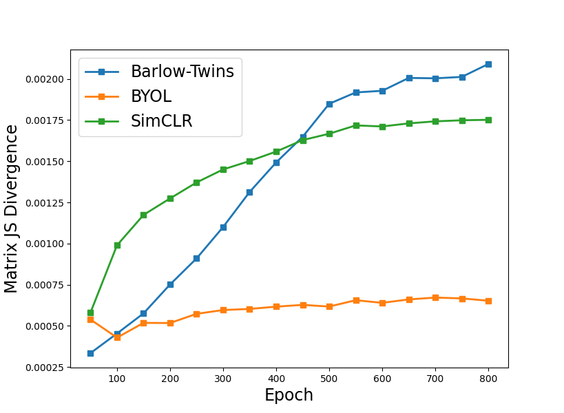
(a) Matrix JS Divergence

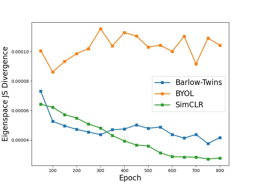
(b) Eigenspace JS Divergence

Figure 3: Visualization of matrix JS divergence and eigenspace JS divergence on CIFAR10 for Barlow-Twins, BYOL and SimCLR.

References

- Arora et al. [2019] Sanjeev Arora, Hrishikesh Khandeparkar, Mikhail Khodak, Orestis Plevrakis, and Nikunj Saunshi. A theoretical analysis of contrastive unsupervised representation learning. In International Conference on Machine Learning, 2019.
- Bach [2022] Francis Bach. Information theory with kernel methods. IEEE Transactions on Information Theory, 2022.
- Bachman et al. [2019] Philip Bachman, R Devon Hjelm, and William Buchwalter. Learning representations by maximizing mutual information across views. arXiv preprint arXiv:1906.00910, 2019.
- Balestriero & LeCun [2022] Randall Balestriero and Yann LeCun. Contrastive and non-contrastive self-supervised learning recover global and local spectral embedding methods. arXiv preprint arXiv:2205.11508, 2022.
- Bardes et al. [2021] Adrien Bardes, Jean Ponce, and Yann LeCun. Vicreg: Variance-invariance-covariance regularization for self-supervised learning. arXiv preprint arXiv:2105.04906, 2021.
- Cabannes et al. [2023] Vivien Cabannes, Bobak T Kiani, Randall Balestriero, Yann LeCun, and Alberto Bietti. The ssl interplay: Augmentations, inductive bias, and generalization. arXiv preprint arXiv:2302.02774, 2023.
- Cao et al. [2022] Shuhao Cao, Peng Xu, and David A Clifton. How to understand masked autoencoders. arXiv preprint arXiv:2202.03670, 2022.
- Caron et al. [2020] Mathilde Caron, Ishan Misra, Julien Mairal, Priya Goyal, Piotr Bojanowski, and Armand Joulin. Unsupervised learning of visual features by contrasting cluster assignments. Advances in Neural Information Processing Systems, 33:9912–9924, 2020.
- Caron et al. [2021] Mathilde Caron, Hugo Touvron, Ishan Misra, Hervé Jégou, Julien Mairal, Piotr Bojanowski, and Armand Joulin. Emerging properties in self-supervised vision transformers. In Proceedings of the IEEE/CVF international conference on computer vision, pp. 9650–9660, 2021.
- Chen et al. [2020] Ting Chen, Simon Kornblith, Mohammad Norouzi, and Geoffrey Hinton. A simple framework for contrastive learning of visual representations. In International Conference on Machine Learning, pp. 1597–1607. PMLR, 2020.
- Chen & He [2021] Xinlei Chen and Kaiming He. Exploring simple siamese representation learning. In Proceedings of the IEEE/CVF conference on Computer Vision and Pattern Recognition, pp. 15750–15758, 2021.
- Deng et al. [2009] Jia Deng, Wei Dong, Richard Socher, Li-Jia Li, Kai Li, and Li Fei-Fei. Imagenet: A large-scale hierarchical image database. In 2009 IEEE conference on computer vision and pattern recognition, pp. 248–255. Ieee, 2009.
- Devlin et al. [2018] Jacob Devlin, Ming-Wei Chang, Kenton Lee, and Kristina Toutanova. Bert: Pre-training of deep bidirectional transformers for language understanding. arXiv preprint arXiv:1810.04805, 2018.
- Dubois et al. [2022] Yann Dubois, Tatsunori Hashimoto, Stefano Ermon, and Percy Liang. Improving self-supervised learning by characterizing idealized representations. arXiv preprint arXiv:2209.06235, 2022.
- Gao et al. [2021] Tianyu Gao, Xingcheng Yao, and Danqi Chen. Simcse: Simple contrastive learning of sentence embeddings. arXiv preprint arXiv:2104.08821, 2021.
- Garrido et al. [2022] Quentin Garrido, Yubei Chen, Adrien Bardes, Laurent Najman, and Yann Lecun. On the duality between contrastive and non-contrastive self-supervised learning. arXiv preprint arXiv:2206.02574, 2022.
- Garrido et al. [2023] Quentin Garrido, Randall Balestriero, Laurent Najman, and Yann Lecun. Rankme: Assessing the downstream performance of pretrained self-supervised representations by their rank. In International Conference on Machine Learning, pp. 10929–10974. PMLR, 2023.
- Giraldo et al. [2014] Luis Gonzalo Sanchez Giraldo, Murali Rao, and Jose C Principe. Measures of entropy from data using infinitely divisible kernels. IEEE Transactions on Information Theory, 61(1):535–548, 2014.
- Grill et al. [2020] Jean-Bastien Grill, Florian Strub, Florent Altché, Corentin Tallec, Pierre Richemond, Elena Buchatskaya, Carl Doersch, Bernardo Avila Pires, Zhaohan Guo, Mohammad Gheshlaghi Azar, et al. Bootstrap your own latent-a new approach to self-supervised learning. Advances in Neural Iformation Processing Systems, 33:21271–21284, 2020.
- HaoChen & Ma [2022] Jeff Z HaoChen and Tengyu Ma. A theoretical study of inductive biases in contrastive learning. arXiv preprint arXiv:2211.14699, 2022.
- HaoChen et al. [2021] Jeff Z HaoChen, Colin Wei, Adrien Gaidon, and Tengyu Ma. Provable guarantees for self-supervised deep learning with spectral contrastive loss. Advances in Neural Information Processing Systems, 34:5000–5011, 2021.
- HaoChen et al. [2022] Jeff Z. HaoChen, Colin Wei, Ananya Kumar, and Tengyu Ma. Beyond separability: Analyzing the linear transferability of contrastive representations to related subpopulations. Advances in Neural Information Processing Systems, 2022.
- He et al. [2022] Kaiming He, Xinlei Chen, Saining Xie, Yanghao Li, Piotr Dollár, and Ross Girshick. Masked autoencoders are scalable vision learners. In Proceedings of the IEEE/CVF conference on computer vision and pattern recognition, pp. 16000–16009, 2022.
- Henaff [2020] Olivier Henaff. Data-efficient image recognition with contrastive predictive coding. In International Conference on Machine Learning, pp. 4182–4192. PMLR, 2020.
- Hjelm et al. [2018] R Devon Hjelm, Alex Fedorov, Samuel Lavoie-Marchildon, Karan Grewal, Phil Bachman, Adam Trischler, and Yoshua Bengio. Learning deep representations by mutual information estimation and maximization. In International Conference on Learning Representations, 2018.
- Hoyos-Osorio & Sanchez-Giraldo [2023] Jhoan K Hoyos-Osorio and Luis G Sanchez-Giraldo. The representation jensen-shannon divergence. arXiv preprint arXiv:2305.16446, 2023.
- Hu et al. [2022] Tianyang Hu, Zhili Liu, Fengwei Zhou, Wenjia Wang, and Weiran Huang. Your contrastive learning is secretly doing stochastic neighbor embedding. arXiv preprint arXiv:2205.14814, 2022.
- Huang et al. [2021] Weiran Huang, Mingyang Yi, and Xuyang Zhao. Towards the generalization of contrastive self-supervised learning. arXiv preprint arXiv:2111.00743, 2021.
- Kong et al. [2023] Lingjing Kong, Martin Q Ma, Guangyi Chen, Eric P Xing, Yuejie Chi, Louis-Philippe Morency, and Kun Zhang. Understanding masked autoencoders via hierarchical latent variable models. In Proceedings of the IEEE/CVF Conference on Computer Vision and Pattern Recognition, pp. 7918–7928, 2023.
- Lee et al. [2020] Jason D Lee, Qi Lei, Nikunj Saunshi, and Jiacheng Zhuo. Predicting what you already know helps: Provable self-supervised learning. arXiv preprint arXiv:2008.01064, 2020.
- Lee et al. [2021] Jason D Lee, Qi Lei, Nikunj Saunshi, and Jiacheng Zhuo. Predicting what you already know helps: Provable self-supervised learning. Advances in Neural Information Processing Systems, 34:309–323, 2021.
- Li et al. [2021] Yazhe Li, Roman Pogodin, Danica J Sutherland, and Arthur Gretton. Self-supervised learning with kernel dependence maximization. Advances in Neural Information Processing Systems, 34:15543–15556, 2021.
- Misra & Maaten [2020] Ishan Misra and Laurens van der Maaten. Self-supervised learning of pretext-invariant representations. In Proceedings of the IEEE/CVF Conference on Computer Vision and Pattern Recognition, pp. 6707–6717, 2020.
- Nozawa & Sato [2021] Kento Nozawa and Issei Sato. Understanding negative samples in instance discriminative self-supervised representation learning. Advances in Neural Information Processing Systems, 34:5784–5797, 2021.
- Oord et al. [2018] Aaron van den Oord, Yazhe Li, and Oriol Vinyals. Representation learning with contrastive predictive coding. arXiv preprint arXiv:1807.03748, 2018.
- Pokle et al. [2022] Ashwini Pokle, Jinjin Tian, Yuchen Li, and Andrej Risteski. Contrasting the landscape of contrastive and non-contrastive learning. arXiv preprint arXiv:2203.15702, 2022.
- Robinson et al. [2021] Joshua David Robinson, Ching-Yao Chuang, Suvrit Sra, and Stefanie Jegelka. Contrastive learning with hard negative samples. In ICLR, 2021.
- Roy & Vetterli [2007] Olivier Roy and Martin Vetterli. The effective rank: A measure of effective dimensionality. In 2007 15th European signal processing conference, pp. 606–610. IEEE, 2007.
- Saunshi et al. [2022] Nikunj Saunshi, Jordan Ash, Surbhi Goel, Dipendra Misra, Cyril Zhang, Sanjeev Arora, Sham Kakade, and Akshay Krishnamurthy. Understanding contrastive learning requires incorporating inductive biases. In International Conference on Machine Learning, pp. 19250–19286. PMLR, 2022.
- Shwartz-Ziv & LeCun [2023] Ravid Shwartz-Ziv and Yann LeCun. To compress or not to compress–self-supervised learning and information theory: A review. arXiv preprint arXiv:2304.09355, 2023.
- Shwartz-Ziv et al. [2023] Ravid Shwartz-Ziv, Randall Balestriero, Kenji Kawaguchi, Tim GJ Rudner, and Yann LeCun. An information-theoretic perspective on variance-invariance-covariance regularization. arXiv preprint arXiv:2303.00633, 2023.
- Skean et al. [2023] Oscar Skean, Jhoan Keider Hoyos Osorio, Austin J Brockmeier, and Luis Gonzalo Sanchez Giraldo. Dime: Maximizing mutual information by a difference of matrix-based entropies. arXiv preprint arXiv:2301.08164, 2023.
- Sordoni et al. [2021] Alessandro Sordoni, Nouha Dziri, Hannes Schulz, Geoff Gordon, Philip Bachman, and Remi Tachet Des Combes. Decomposed mutual information estimation for contrastive representation learning. In International Conference on Machine Learning, pp. 9859–9869. PMLR, 2021.
- Tan et al. [2023] Zhiquan Tan, Yifan Zhang, Jingqin Yang, and Yang Yuan. Contrastive learning is spectral clustering on similarity graph. arXiv preprint arXiv:2303.15103, 2023.
- Tao et al. [2022] Chenxin Tao, Honghui Wang, Xizhou Zhu, Jiahua Dong, Shiji Song, Gao Huang, and Jifeng Dai. Exploring the equivalence of siamese self-supervised learning via a unified gradient framework. In Proceedings of the IEEE/CVF Conference on Computer Vision and Pattern Recognition, pp. 14431–14440, 2022.
- Tian et al. [2019] Yonglong Tian, Dilip Krishnan, and Phillip Isola. Contrastive multiview coding. arXiv preprint arXiv:1906.05849, 2019.
- Tian et al. [2020] Yonglong Tian, Chen Sun, Ben Poole, Dilip Krishnan, Cordelia Schmid, and Phillip Isola. What makes for good views for contrastive learning. arXiv preprint arXiv:2005.10243, 2020.
- Tian [2022] Yuandong Tian. Deep contrastive learning is provably (almost) principal component analysis. arXiv preprint arXiv:2201.12680, 2022.
- Tian et al. [2021] Yuandong Tian, Xinlei Chen, and Surya Ganguli. Understanding self-supervised learning dynamics without contrastive pairs. In International Conference on Machine Learning, pp. 10268–10278. PMLR, 2021.
- Tosh et al. [2020] Christopher Tosh, Akshay Krishnamurthy, and Daniel Hsu. Contrastive estimation reveals topic posterior information to linear models. arXiv:2003.02234, 2020.
- Tosh et al. [2021] Christopher Tosh, Akshay Krishnamurthy, and Daniel Hsu. Contrastive learning, multi-view redundancy, and linear models. In Algorithmic Learning Theory, pp. 1179–1206. PMLR, 2021.
- Tsai et al. [2021] Yao-Hung Hubert Tsai, Shaojie Bai, Louis-Philippe Morency, and Ruslan Salakhutdinov. A note on connecting barlow twins with negative-sample-free contrastive learning. arXiv preprint arXiv:2104.13712, 2021.
- Wang & Isola [2020] Tongzhou Wang and Phillip Isola. Understanding contrastive representation learning through alignment and uniformity on the hypersphere. In International Conference on Machine Learning, pp. 9929–9939. PMLR, 2020.
- Wang et al. [2022] Yifei Wang, Qi Zhang, Yisen Wang, Jiansheng Yang, and Zhouchen Lin. Chaos is a ladder: A new theoretical understanding of contrastive learning via augmentation overlap. arXiv preprint arXiv:2203.13457, 2022.
- Wen & Li [2021] Zixin Wen and Yuanzhi Li. Toward understanding the feature learning process of self-supervised contrastive learning. In International Conference on Machine Learning, pp. 11112–11122. PMLR, 2021.
- Wen & Li [2022] Zixin Wen and Yuanzhi Li. The mechanism of prediction head in non-contrastive self-supervised learning. arXiv preprint arXiv:2205.06226, 2022.
- Wu et al. [2018] Zhirong Wu, Yuanjun Xiong, Stella X Yu, and Dahua Lin. Unsupervised feature learning via non-parametric instance discrimination. In Proceedings of the IEEE Conference on Computer Vision and Pattern Recognition, pp. 3733–3742, 2018.
- Xie et al. [2022] Zhenda Xie, Zheng Zhang, Yue Cao, Yutong Lin, Jianmin Bao, Zhuliang Yao, Qi Dai, and Han Hu. Simmim: A simple framework for masked image modeling. In Proceedings of the IEEE/CVF Conference on Computer Vision and Pattern Recognition, pp. 9653–9663, 2022.
- Ye et al. [2019] Mang Ye, Xu Zhang, Pong C Yuen, and Shih-Fu Chang. Unsupervised embedding learning via invariant and spreading instance feature. In Proceedings of the IEEE/CVF Conference on Computer Vision and Pattern Recognition, pp. 6210–6219, 2019.
- Yu et al. [2020] Yaodong Yu, Kwan Ho Ryan Chan, Chong You, Chaobing Song, and Yi Ma. Learning diverse and discriminative representations via the principle of maximal coding rate reduction. Advances in Neural Information Processing Systems, 33:9422–9434, 2020.
- Zbontar et al. [2021] Jure Zbontar, Li Jing, Ishan Misra, Yann LeCun, and Stéphane Deny. Barlow twins: Self-supervised learning via redundancy reduction. In International Conference on Machine Learning, pp. 12310–12320. PMLR, 2021.
- Zhang et al. [2022] Qi Zhang, Yifei Wang, and Yisen Wang. How mask matters: Towards theoretical understandings of masked autoencoders. Advances in Neural Information Processing Systems, 35:27127–27139, 2022.
- Zhang et al. [2023a] Yifan Zhang, Zhiquan Tan, Jingqin Yang, Weiran Huang, and Yang Yuan. Matrix information theory for self-supervised learning. arXiv preprint arXiv:2305.17326, 2023a.
- Zhang et al. [2023b] Yifan Zhang, Jingqin Yang, Zhiquan Tan, and Yang Yuan. Relationmatch: Matching in-batch relationships for semi-supervised learning. arXiv preprint arXiv:2305.10397, 2023b.
- Zhou et al. [2021] Jinghao Zhou, Chen Wei, Huiyu Wang, Wei Shen, Cihang Xie, Alan Yuille, and Tao Kong. ibot: Image bert pre-training with online tokenizer. arXiv preprint arXiv:2111.07832, 2021.