Continual Action Assessment via Task-Consistent Score-Discriminative Feature Distribution Modeling

Abstract

Action Quality Assessment (AQA) is a task that tries to answer how well an action is carried out. While remarkable progress has been achieved, existing works on AQA assume that all the training data are visible for training in one time, but do not enable continual learning on assessing new technical actions. In this work, we address such a Continual Learning problem in AQA (Continual-AQA), which urges a unified model to learn AQA tasks sequentially without forgetting. Our idea for modeling Continual-AQA is to sequentially learn a task-consistent score-discriminative feature distribution, in which the latent features express a strong correlation with the score labels regardless of the task or action types. From this perspective, we aim to mitigate the forgetting in Continual-AQA from two aspects. Firstly, to fuse the features of new and previous data into a score-discriminative distribution, a novel Feature-Score Correlation-Aware Rehearsal is proposed to store and reuse data from previous tasks with limited memory size. Secondly, an Action General-Specific Graph is developed to learn and decouple the action-general and action-specific knowledge so that the task-consistent score-discriminative features can be better extracted across various tasks. Extensive experiments are conducted to evaluate the contributions of proposed components. The comparisons with the existing continual learning methods additionally verify the effectiveness and versatility of our approach.

I Introduction

Action Quality Assessment (AQA) aims to assess the quality of action in videos. Rather than classifying the video samples by their action types [1, 2, 3], a common setting of AQA is to predict a subtle action quality score for a video action instance. Recently, AQA has attached more and more attention for its great potential value for sports skills analysis [4, 5, 6, 7], surgical maneuver training [8, 9, 10] and so on[11, 12].

Although remarkable progress has been achieved, a remaining challenge in AQA has yet to be explored. In practical application, the increasing demand drives the model to sequentially expand its applicability on different tasks (e.g., new technical actions or various daily actions). A more practical example is that, considering someday you may hope your AI cooking assistant can guide you on how to complete a French dish, but currently, it may only assess how well you cook Japanese cuisine. However, existing works on AQA assume that all the training data are visible for training at one time, ignoring such increasing demands. The already trained model may not work on the newly come tasks, resulting in misjudging or misguiding.

In this work, we consider a more complex but real scenario, Continual Learning (CL) in AQA, namely Continual-AQA. Like the other deep neural networks, AQA models also suffer from Catastrophic Forgetting[13, 14, 15]. As shown in Figure 1, when directly fine-tuning an already trained model from one AQA task to another, the performance significantly drops no matter adapting the model to a dissimilar task (e.g., Sync.3m and Skiing are quite not similar) or even a similar one (e.g., both Sync.3m and Single.10m are diving-like actions).

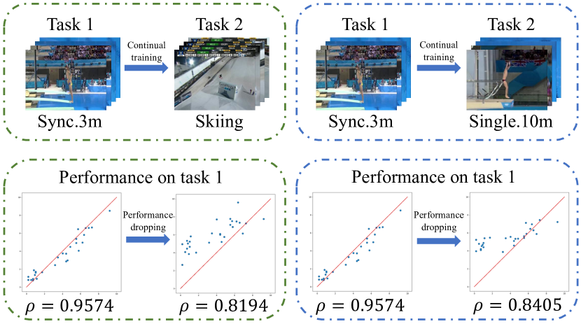
Figure 1: Catastrophic forgetting in Continual-AQA. We sequentially train an AQA model on two tasks and show the performance on the first task in scatter plot and Spearman’s rank correlation coefficient ($\rho$). A higher $\rho$ (i.e., more points close to the red lines) indicates better performance.

To mitigate the forgetting, we start by analyzing the different learning targets between Conventional CL and Continual-AQA. As shown in Figure 2, we claim that to solve Continual-AQA, the key is to sequentially construct a task-consistent score-discriminative feature distribution across all seen tasks rather than learning disjoint feature clusters and decision boundaries for different classes or tasks in conventional CL [16, 17, 18]. A further explanation of this claim is that if an AQA model can map video actions of seen tasks to the feature space, in which the latent features express a strong correlation with the score labels regardless of the task or action types, it would be able to handle various tasks without forgetting. Moreover, considering different AQA tasks have general and specific assessing criteria (e.g., body balance and motion fluency are general criteria; landing distance and splash are specific criteria for Snowboarding and Diving, respectively), it is challenging to extract task-consistent score-discriminative features without explicitly modeling such general and specific knowledge. Therefore, to achieve Continual-AQA with less forgetting, we raise the two following problems: 1) How to fuse rather than isolate the previously learned feature distribution with the newly learned one? 2) How to explicitly model general and specific knowledge across tasks so that consistent score-discriminative features can be better extracted?

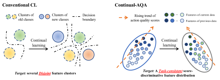
Figure 2: Different learning targets of Conventional Continual Learning and Continual-AQA. The learning target of conventional Continual Learning (left) is to construct new decision boundaries so that intra-class features can be clustered and inter-class features can be separated. Differently, the learning target of Continual-AQA (right) is to learn a task-consistent score-discriminative feature distribution where the features strongly correlate with the score labels regardless of the task or action types.

To address the problems above, we propose a novel Feature-Score Correlation-Aware Rehearsal (FSCAR) to store and reuse data from previous tasks with limited memory size. First, to sample representative exemplars, an intuitive but effective Grouping Sampling strategy is adopted to sample exemplars that cover different score levels. Additionally, to address the problem that the model would prefer to learn data from the current task due to the imbalance of previous and current data [18, 19, 20], a Feature-Score co-Augmentation is proposed to augment the latent features and the scores of previous data. We introduce the concept of “augmentation helpers”, which provide information on the feature distribution of previous data so that the augmentation can be guided and the augmented feature distribution can correctly reflect the correlation between features and action quality scores. Moreover, an alignment loss based on difference modeling [21] is adopted to align the features across tasks and construct a task-consistent score-discriminative feature distribution.

Furthermore, we separately model the action-general and action-specific knowledge to better extract consistent score-discriminative features across different tasks). Specifically, we build an Action General-Specific Graph (AGSG) over the original joint relation graph proposed in [4]. AGSG decouples the original joint relation graph into two parts (i.e., Action General Graph and Action Specific Graph) to model action-general and action-specific knowledge, respectively. We observe that such a design can further mitigate forgetting.

In summary, the contributions of our works are as follows: 1) To our best knowledge, this is the first work to study Continual-AQA. 2) We propose a novel Feature-Score Correlation-Aware Rehearsal (FSCAR) to store and reuse data from previous tasks. Compared with existing rehearsal-based methods, FSCAR is more suitable for Continual-AQA with its feature-score correlation awareness. 3) We propose to learn and decouple action-general and action-specific knowledge with an Action General-Specific Graph module for learning different AQA tasks sequentially with less forgetting.

Extensive experiments are conducted, and the results show that: 1) Compared with directly fine-tuning the model sequentially, our approach explicitly mitigates the forgetting in Continual-AQA. 2) Our approach outperforms other possible variants, the existing general CL approaches [22, 16, 23, 24] and successful AQA methods [25, 21] trained with naive CL solutions. 3) Our approach has versatility in various Continual-AQA scenarios.

II Related Works

Action Quality Assessment (AQA) aims to evaluate and quantify the overall performance or proficiency of human actions based on video or motion data analysis. Most works in AQA mainly focus on problem formulations [11, 25, 21, 6, 26], designing effective feature extractors [7, 12, 4, 27, 28, 29, 30], data insufficiency [31, 32], and so on. However, most existing methods only consider training the model at one time, ignoring the problem of training a model continually. In this paper, considering the characteristics of Continual-AQA, we attempt to find a feasible solution for this problem.

The closest to our work is [4] because our AGSG is built on the proposed JRG module. However, the original JRG is not designed for Continual Learning, and AGSG differs from it in graph calculation and model training. Additionally, a concurrent work [33] considers the transferable knowledge across various tasks and tries to model such knowledge explicitly, but it assumes that data from different tasks are all available during training, which contradicts the invisibility of previous data in Continual-AQA.

Continual Learning (CL) is a rising research direction to study how to train deep neural networks sequentially. The main problem in CL is that the model will forget the previously learned knowledge when learning new knowledge, namely catastrophic forgetting.

To address catastrophic forgetting, Rehearsal-based methods propose to save and reuse several samples of older tasks. In the past few years, many methods [16, 18, 19, 20, 24] focused on selecting representative exemplars and balancing new and limited old data. However, compared with convention classification-based CL, Continual-AQA has a totally different learning target, which makes the existing methods [16, 18, 19, 20] unsuitable for Continual-AQA with their classification-based designs. In this work, a novel rehearsal-based method is proposed considering the distinct learning target explained in Figure 2. Recently, inspired by Complementary Learning, some works [34, 17] propose to model task-invariant and task-specific knowledge to address catastrophic forgetting. However, existing works either heavily rely on pre-training [34] or attempts to construct a disjoint representation for the private knowledge of each task [17]. In this work, we address Continual-AQA without any pre-training on other AQA tasks. Additionally, we design an Action General-Specific Graph module to extract general and specific knowledge to map the input video actions from different tasks to the features in a task-consistent action quality latent space.

III Problem Formulation

We first review the general setting of AQA: given a video instance that contains one action (e.g., diving or skiing) to be assessed, the model is expected to predict the action quality score of the action. Following existing works [35, 4, 7, 36], we formulate AQA as a regression-based task.

Now considering a sequence of AQA tasks $D=\{D^{1},...,D^{T}\}$, the $t$-th task $D^{t}$ contains $N^{t}$ video instances $v^{t}$ and their action quality scores. Tasks with various action types (e.g., Diving and Snowboard) will arrive sequentially, and the model will be trained each time a new task arrives. When training the model on a new task $D^{t}$, data from previous tasks will not be available, or just a tiny amount (less than a predefined small number $M$) of them can be stored and reused. The goal of Continual-AQA is to train a unified model $F_{\theta}:V\to S$ parameterized by $\theta$, so that it can predict the action quality score $\hat{s}=F_{\theta}(v)\in S$ correctly when given an unseen test video action $v$ from any task has been seen before. In this work, we separate the model into a feature extractor $E$ and a lightweight score regressor $R_{s}$, which means $\hat{s}=F_{\theta}(v)=R_{s}(E(v))$.

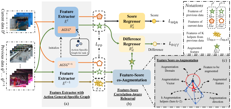
Figure 3: A pipeline of our method for Continual-AQA. Our framework contains two main components: Feature-Score Correlation-Aware Rehearsal(FSCAR) in sub-image (b) and Feature Extractor with Action General-Specific Graph(AGSG) in sub-image (a). Notably, when a new task comes, the model is initialized by the previously learned weights, and a new Action-Specific Graph will be defined for the new task before training. An intuitive example of Feature-Score co-Augmentation is shown in sub-image (c), where a feature with a darker color has a higher quality score. Arrows in different colors indicate different data streams. $\{1,...,t\}$ is the index of tasks and here we denote task $t$ is the current task and task $t\text{-}1$ is the nearest previous task. $D^{t}$ denotes all the training data in current task, and $\psi=\{\psi^{1},...,\psi^{t-1}\}$ denotes the stored exemplars of previous tasks. Best viewed in color.

IV Methodology

IV-A Overview of Our Method

As illustrated in Section I, Continual-AQA has a different learning target from conventional Classification-based Continual Learning, that is, learning a task-consistent score-discriminative feature distribution across all seen tasks. Motivated by this, two main questions have been raised: 1) How to fuse rather than isolate the previously learned feature distribution with the newly learned one? 2) How to model the general and specific knowledge so that score-discriminative features can be better extracted across tasks? To address the two questions, we develop our method from the following two aspects.

For the first question, we propose a novel rehearsal-based method, namely Feature-Score Correlation-Aware Rehearsal (FSCAR), which includes: 1) a Grouping Sampling strategy to sample representative exemplars; 2) a Feature-Score co-Augmentation to augment the previous data so that the imbalance problem can be addressed; 3) a different modeling-based feature alignment loss function $\mathcal{L}_{Diff}$ to align the feature of previous and current data into a task-consistent feature distribution.

For the second question, we propose Action General-Specific Graph (AGSG), which can be shown as the lower part of Figure 4, to strengthen the ability to extract task-consistent features of the feature extractor during continual training. AGSG contains an Action-General Graph and an Action-Specific Graph to learn action-general and action-specific knowledge, respectively. Moreover, a distillation-based loss function $\mathcal{L}_{FD}$ is proposed for AGSG to maintain and decouple the already learned knowledge during continual training.

Figure 3 illustrates the overall framework of our method. In the following part of this section, we will introduce FSCAR and AGSG in Section IV-B and Section IV-C, respectively. After that, the details about continual training strategies will be introduced in Section IV-D.

IV-B Feature-Score Correlation-Aware Rehearsal

In Continual-AQA, an ideal way to reuse insufficient previous data is to give an adequate description of the already learned feature distribution and fuse the feature of the old and new data into a task-consistent score-discriminative distribution so that the regressor can perform an accurate prediction on the scores regardless of the action types. To this end, we propose a Feature-Score Correlation-Aware Rehearsal, which mainly solves two problems: ”what to replay” and “how to replay” for Continual-AQA.

After training on task ${t\text{-}1}$, we adopt a Grouping Sampling (GS) strategy to sample representative exemplars of task $t\text{-}1$. Suppose we need to sample $m$ exemplars to store in the memory of size M and reuse them in the future training stages. GS first uniformly separates data into $m$ groups based on the score ranking. After that, one exemplar will be sampled from each group. The sampled exemplars of task $t\text{-}1$ are denoted as $\psi_{t-1}$. Although such a sampling strategy is intuitive, experiments in Section V-D show that it can already roughly describe the relationship between video action instances and quality scores and cover exemplars with different-level scores for previous data.

To reuse the stored data and solve the imbalance problem [18, 19, 20], when training on task $t$ ($t>1$), the stored exemplars of previous tasks $\{\psi^{1},...,\psi^{t-1}\}$ are fed into feature extractor $E^{t}$ and $E^{t-1}$. Suppose $f_{pre,j}^{t}$ and $f_{pre,j}^{t-1}$ denote the features of a previous instance extracted by $E^{t}$ and $E^{t-1}$. Then, a Feature-Score co-Augmentation(FS-Aug) is applied on $f_{pre,j}^{t-1}$ and its corresponding action quality score $s_{pre,j}$ to obtain the augmented feature $\tilde{f}^{t-1}_{pre,j}$ and score $\tilde{s}_{pre,j}$. Explicitly, given a feature to be augmented and its corresponding action quality score, FS-Aug first randomly selects K feature-score pairs from previous data as the augmentation helpers, which can be denoted as $H_{feat}=\{f_{hlp,1}^{t-1},...,f_{hlp,K}^{t-1}\}$ and $H_{score}=\{s_{hlp,1},...,s_{hlp,K}\}$. Then, the feature perturbation $\Delta f$ and the score perturbation $\Delta s$ are computed as:

$$\Delta f_{j}=\frac{1}{K}\sum_{k=1}^{K}f^{t-1}_{hlp,k}-f_{pre,j}^{t-1},$$ (1)

$$\Delta s_{j}=\frac{1}{K}\sum_{k=1}^{K}s_{hlp,k}-s_{pre,j}.$$ (2)

Given the perturbations, the augmented feature and score can be computed as:

$$\tilde{f}^{t-1}_{pre,j}=f_{pre,j}^{t-1}+\varepsilon\Delta f_{j},$$ (3)

$$\tilde{s}_{pre,j}=s_{pre,j}+\varepsilon\Delta s_{j},$$ (4)

where $\varepsilon$ is sampled from a Gaussian distribution $N(0,\sigma)$ and $\sigma$ is a hyper-parameter.

Finally, an auxiliary loss is adopted to align the features of previous and current data into a consistent distribution. Specifically, inspired by the idea of score difference modeling proposed in CoRe [21], an auxiliary difference regressor $R^{t}_{d}$ is utilized to predict the score difference between $\tilde{f}^{t-1}_{pre}$ and $f_{pre}^{t}$, and the difference loss is computed as:

$$d=\tilde{s}_{pre}-s_{pre},$$ (5)

$$L_{Diff}=(R^{t}_{d}(\tilde{f}^{t-1}_{pre,j}\copyright f_{pre,j}^{t})-d)^{2},$$ (6)

where $\copyright$ denotes the concatenation operation.

- Discussions. It has been emphasized in previous works [18, 19, 20] that the imbalance of previous and current data will cause forgetting. Hence, inspired by PASS [18], besides training $R^{t}_{s}$ with current data and stored previous data, we propose FS-Aug to augment previous data to address the imbalance issue. We have to claim that augmenting the corresponding scores together with the features is necessary because of the strong correlation between features and scores, which means a subtle perturbation in features would cause a perturbation in scores. Noting that PASS [18] augments feature by adding random Gaussian noise, it is impossible for PASS to perceive such a strong correlation. Differently, in our FS-Aug, augmentation helpers are introduced to provide information on the subtle correlation between latent features and scores so that the augmentation can be guided. Moreover, we adopt a difference modeling-based loss to maintain the score-discriminability of $\tilde{f}^{t-1}_{pre,j}$ and $f_{pre,j}^{t}$ given any $i$ so that the forgetting can be constrained. Ablation studies in Sec. V-D show that our approach outperforms the augmentation method proposed in PASS [18] and other possible strategies.

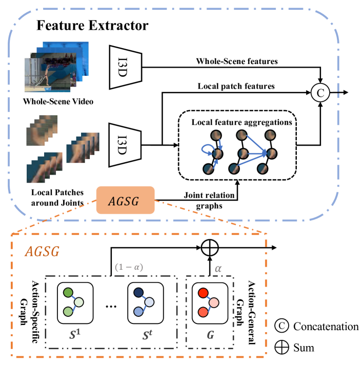
Figure 4: Feature extractor with the proposed Action General-Specific Graph (AGSG). Different from the original JRG[4], in this work, we decouple the original joint relation graph into an Action-General Graph and an Action-Specific Graph to learn action-general and action-specific knowledge, respectively (the lower part).

IV-C Action General-Specific Graph

Considering the shared and specific criteria across various AQA tasks, we build our general-specific knowledge Modeling module, namely Action General-Specific Graph (AGSG), on JRG [4] to learn and decouple action-general and action-specific knowledge so that task-consistent features can be better extracted. The pipeline of AGSG can be shown in Figure 4.

Following [4], we define a joint relation graph as a learnable weight matrix $A\in\mathbb{R}^{J\times J}$, where $J$ denotes the number of joints. An element $A[i,j]$ denotes the importance of the relationship between the $i$-th and $j$-th joint for assessing one type of action. In our work, AGSG contains a set of Action-Specific Graphs (ASG) and an Action-General Graph (AGG). An ASG is defined and learned for a single task, and the AGG is shared across different tasks during continual training. Given a task $t$, the AGSG can be computed as:

$$A^{t}=\alpha*G+(1-\alpha)*S^{t},$$ (7)

where $\alpha\in[0,1]$ is a hyperparameter, $G$ denotes the AGG and $S^{t}$ denotes the ASG.

As to the optimization of AGSG, there are two aspects to be considered. First, it is expected that the newly learned feature extractor can output similar features as the previously learned one to maintain the learned knowledge. Second, the action-general and action-specific knowledge are expected to be decoupled during continual training. To address these, we do not freeze AGG and ASG during the continual training stages and conduct a distillation-based loss function $\mathcal{L}_{FD}$ on the output features obtained from $E^{t}$ and $E^{t-1}$. Specifically, given a video instance of $v^{\epsilon}_{i}$ from a seen but agnostic task $\epsilon$, we use the features extracted by $E^{t-1}$ as the distillation target and $\mathcal{L}_{FD}$ can be written as:

$$\mathcal{L}_{FD}=\sum^{t-1}_{g=1}||E^{t}_{g}(v^{*}_{i})-E^{t-1}_{g}(v^{*}_{i})||^{2}.$$ (8)

Here we introduce the subscript $g\in\{1,...,t-1\}$ for $E^{t}$ and $E^{t-1}$ to denote that $A^{g}$ is utilized to extract features. Although those features extracted when using AGSGs except $A^{\epsilon}$ are meaningless for the inference stage, inspired by LwF [37], we believe they are valuable as pseudo labels for distillation.

Noting that it is essential to keep the model initialized in an identical way for fair comparisons, and a better initialization can help a model learn better. Hence, at the base step ($t\text{=}1$), we initialize the ASG to keep the initial $A^{1}$ the same as those in the model without ASG. At continual training steps, we initialize $S^{t}$ by the previously learnt ASG at task $t\text{-}1$. Experiments in Sec. V-E show that such initialization can gain performance improvement.

- Discussions. We develop a stronger feature extractor rather than directly adopting the original JRG [4] for the following two reasons. First, the importance of the relationship between joint pairs may differ among actions, for which using a single graph to model joint relationships across different actions is not feasible for Continual-AQA. Second, considering the general and specific judging criteria across different tasks, action-general and action-specific knowledge should be explicitly modeled. Hence, AGSG is proposed to model such dual knowledge during continual training. We believe modeling and decoupling the general and specific knowledge across various tasks would further mitigate forgetting because the general knowledge can be shared, and the specific knowledge can be isolated so that task-consistent features can be better extracted. Notably, the AGSG module has two-fold novelties: 1) Compared with the existing works on AQA, AGSG is the first module explicitly models general and specific knowledge. 2) Compared with the original JRG, AGSG is a CL-based module that differs from JRG in graph calculation and model training.

IV-D Continual Training Strategy

As introduced in IV-B, FS-Aug directly augments $f_{pre,j}^{t-1}$ and $s_{pre,j}$. Therefore, instead of mixing the previous data and current data together, given a mini-batch size $b$ for current data, we additionally sample a mini-batch from previous data to compute $f_{pre,j}^{t}$ and $f_{pre,j}^{t-1}$. Moreover, during training, given an instance $v^{\epsilon}_{i}$ from task $\epsilon$, $f^{t}$ and $f^{t-1}$ introduced in Section IV-B are extracted using the AGSG $A^{\epsilon}$.

To sum up, the complete loss function during training can be written as:

$$\mathcal{L}=\mathcal{L}_{AQA}+\lambda_{FD}\mathcal{L}_{FD}+\lambda_{Diff}\mathcal{L}_{Diff},$$ (9)

where $\lambda_{FD}$ and $\lambda_{Diff}$ are hyper-parameters. Following previous works [4, 26], AQA loss is defined as the MSE loss across the predicted and ground-truth scores. Note that when training the model on the first task, the later two losses are not computed to optimize the model. For more training details, please refer to Algorithm 1.

V Experiments

In this section, we first introduce the datasets and evaluation metrics for Continual-AQA, then describe our implementation details. After that, we perform ablation studies to analyze our model in detail. Finally, comparisons are conducted between the proposed method and other baselines.

V-A Datasets and Evaluation Metrics

- Continual-AQA Datasets. We conduct experiments to evaluate our model on three public action quality assessment datasets: the AQA-7 dataset [38], the MTL-AQA dataset [26], and the BEST dataset [12]. The introductions of the datasets are as follows:

AQA-7 [38]: The AQA-7 dataset contains 1,189 videos from seven summer- and winder-Olympic Games: single diving-10m platform (Diving), gymnastic vault (Gym vault), synchronous diving-3m springboard (Sync.3m), synchronous diving-10m platform, big air skiing (Skiing), big air snowboarding (Snowboard) and Trampoline. Following the previous works [21, 4, 25], only the videos from the former six games are used in our work.

MTL-AQA [26]: The MTL-AQA dataset contains 1,412 video actions from 16 different world diving events. As for the annotations, the MTL-AQA contains various annotations, including difficulty, action type, scores from each judge, final scores, and video captions. Only the final scores are used in our work.

BEST [12]: The BEST is a long video dataset with annotations about the relative rankings of video pairs. Detailly, the BEST dataset contains 16,782 video pairs from five various daily actions (i.e., applying eyeliner, braiding hair, folding origami, scrambling eggs and tying a tie).

- Common AQA Metrics. In previous works [35, 21, 6, 12, 11], Pairwise Accuracy and Spearman’s rank correlation coefficient (SRCC) are utilized to evaluate the performance of the model on an AQA task. The Pairwise Accuracy represents the percentage of correctly ranked pairs. The SRCC can evaluate the correlation between the scores series predicted by the model and the ground-truth scores series, which is defined as follows:

$$\rho=\frac{\sum^{N}_{i=1}(x_{i}-\bar{x})(y_{i}-\bar{y})}{\sqrt{\sum^{N}_{i=1}(x_{i}-\bar{x})^{2}\sum^{N}_{i=1}(y_{i}-\bar{y})^{2}}},$$ (10)

where $x$ and ${y}$ are the rankings of the two series.

Following previous works [35, 26, 12], we use SRCC when the experiments are conducted on the AQA-7 and the MTL-AQA datasets and pairwise accuracy when experiments are conducted on the BEST dataset.

- Continual-AQA Metrics. In this work, we utilize Average Performance ($\mathcal{AP}$), Negative Backward Transfer ($\mathcal{NBT}$), and Maximum Forgetting ($\mathcal{MF}$) to evaluate the Continual-AQA models. After training $T$ tasks, an upper triangular performance matrix $P$ can be obtained, and the three metrics can be computed as:

$$\mathcal{AP}=Average(P_{T,1},...,P_{T,T}),$$ (11)

$$\mathcal{NBT}=\frac{1}{T-1}\sum^{T-1}_{t=1}max(0,P_{t,t}-P_{T,t}),$$ (12)

$$\mathcal{MF}=\frac{1}{T-1}\sum^{T-1}_{t=1}\max_{i,j\in\{1,...,T\}}(P_{i,t}-P_{j,t}),\forall j\neq t,$$ (13)

where $P_{i,j}$ denotes the performance on task $j$ after training on task $i$.

$\mathcal{AP}$ evaluates the average performance on all seen tasks, and a higher value indicates better performance. $\mathcal{NBT}$ and $\mathcal{MF}$ evaluate the forgetting during training, and a lower value indicates better performance.

V-B Implementation Details

- Data Preprocessing. For the AQA-7 dataset, we separate it into six non-overlapping subsets according to the type of actions to conduct experiments in a multi-stage training manner. We follow [35] to extract I3D [1] features from raw videos and optical flows in advance.

For the MTL-AQA dataset, we separate it into two subsets (i.e., 3m-springboard and 10m-platform) based on the type of action, which means the number of tasks is 2. Note that under this setting, in the experiments, the values of $\mathcal{NBT}$ are always equal to the values of $\mathcal{MF}$. Hence, in the main paper, only the results on $\mathcal{AP}$ and $\mathcal{NBT}$ are reported in Table 8. We follow [31] to extract I3D [1] features from raw videos and optical flows in advance.

For the BEST dataset, we separate it into five non-overlapping subsets according to the type of actions and directly use the features extracted by the original work [12].

- Model Details. For experiments on the AQA-7 dataset, We follow [4] to build our model except for the graph calculation. We separate the original model into two parts: a feature extractor and a score regressor. The difference regressor in our model has a similar architecture as the score regressor except for the input dimension.

For experiments on the MTL-AQA dataset, We adopt an I3D-LSTM as the feature extractor. The I3D backbone is initialized by the pre-trained weights on the Kinetic-400 dataset [1] and frozen during training. Two layers of LSTMs are adopted to aggregate temporal features and trained from scratch. We adopt this setting for the following two reasons. First, human joint annotations are not provided in the MTL-AQA dataset, and it is impossible to build the JRG-based feature extractor directly. Second, we attempt to study whether our FSCAR can be plugged into other feature extractors and works well.

For experiments on the BEST dataset, We build our model based on the model proposed for the BEST dataset in [35]. In our work, we replace the original NAS-based [39] architecture with a JRG-like module to model the local temporal information.

- Training Settings. In our work, Adam [40] is used to optimize our model. We set the learning rate as 0.01 for AGG and ASG and 0.001 for the other parameters in our model with a $10^{-5}$ weight decay. For our Grouping Sampling, we sample the first exemplar for the former $m\text{-}1$ groups and the last exemplar for the $m$-th group to cover the highest and lowest scores. We set the total memory size $M$ to 30 unless specified otherwise. Following iCaRL [16], we gradually remove exemplars in memory to store new exemplars. To mitigate the influence of specific task orders, for experiments on the AQA-7 and the BEST dataset, we use four random seeds to generate four task sequences. For the MTL-AQA dataset, we conduct experiments on two possible task sequences. The reported results are average performance on different task sequences.

- Existing CL Baselines. In Section V-F, we compare the proposed method with four existing CL methods, including EWC [22], iCaRL [16], PODNet [24] and AFC [23]. The introduction and processing details of the baseline models are as follows:

EWC [22]: Following the original EWC, we conduct a regularization term to constrain the change of the parameters learned from previous tasks.

iCaRL [16]: In this work, we only adopt the Herding strategy to construct the exemplar set without utilizing the NME classifier as the head of the network because it does not work on AQA tasks.

PODNet [24]: In this work, we only adopt the POD loss in the original PODNet to balance previous and current knowledge without utilizing the Local-similarity Classifier as the head of the network because it does not work on AQA tasks.

AFC [23]: Following the original AFC, we compute an “importance” term to adjust the distillation term. In the comparison results on the AQA-7 and BEST datasets, the “importance” term is conducted on the POD loss in the PODNet. In the comparison results on the MTL-AQA dataset, the “importance” term is conducted on the feature distillation loss due to the limitation of selection of feature extractor.

We also report results of two other baselines: Finetune (i.e., directly fine-tuning model on each task) and Upper Bound (i.e., jointly training model all all tasks at once).

- Existing AQA Baselines. In Section V-F, we also compare the proposed method with two more existing AQA methods(i.e., USDL [25] and CoRe-GART [21]). The introduction and processing details of the baseline models are as follows:

USDL [25]: USDL tries to address AQA by reformulating it as a Distribution Prediction problem. In this work, we implement two variants: 1) original USDL, which follows the official implementation of USDL to train the model. 2) USDL*, whose I3D backbone is frozen, and only the distribution predictor is trained across tasks.

CoRe-GART [21]: CoRe-GART proposes to address AQA by reformulating it as a Contrastive Regression Problem, that is, regressing the relative scores between query videos and exemplar videos. In this work, we implement CoRe-GART by following the official implementation of it.

V-C Quantitative Results on each Component

Above all, we conduct ablation studies to evaluate the contribution of each proposed component. The proposed approach is built on a naive model which is optimized on the AQA loss $\mathcal{L}_{AQA}$ and a naive version of feature distillation loss, where

$$\mathcal{L}_{FD(Naive)}=||f^{t}-f^{t-1}||^{2}.$$ (14)

When AGSG is used, the $\mathcal{L}_{FD}$ is reformulated as is introduced in Equation 8. As shown in Table I, II, and III, when gradually adopting the proposed components, the performance gets stably improved. Compared with the naive model, our approach significantly improves the average performance and mitigates forgetting of the model on all seen tasks. In addition, comparing the performance on three datasets, we notice that the model achieves lower $\mathcal{AP}$, higher $\mathcal{NBT}$ and $\mathcal{MF}$ on the AQA-7 dataset. This is because the large domain gap of tasks in the AQA-7 dataset (e.g., Sync.3m and Skiing) causes higher forgetting, and some challenging tasks (e.g., Snowboard) cause lower average performance. While on the MTL-AQA dataset, the domain gap between two diving-like actions is small, naturally making the model suffer from less forgetting. As for the BEST dataset, we note that we use different metrics (i.e., pairwise accuracy rather than SRCC) to calculate the $\mathcal{AP}$, $\mathcal{NBT}$ and $\mathcal{MF}$ and there is no extremely challenging task in the dataset, which make the performance looks better.

TABLE I: Ablation studies of the proposed components on the AQA-7 dataset.

$\mathcal{L}_{FD}$	GS	$\mathcal{L}_{Diff}$	AGSG	$\mathcal{AP}(\uparrow)$	$\mathcal{NBT}(\downarrow)$	$\mathcal{MF}(\downarrow)$
✓				0.5501	0.2403	0.3169
✓	✓			0.6265	0.1770	0.2209
✓	✓	✓		0.6404	0.1571	0.1930
✓	✓	✓	✓	0.6492	0.1085	0.1399

TABLE II: Ablation studies of the proposed components on the BEST dataset.

$\mathcal{L}_{FD}$	GS	$\mathcal{L}_{Diff}$	AGSG	$\mathcal{AP}(\uparrow)$	$\mathcal{NBT}(\downarrow)$	$\mathcal{MF}(\downarrow)$
✓				0.6466	0.2115	0.2428
✓	✓			0.7668	0.0608	0.0870
✓	✓	✓		0.7857	0.0372	0.0456
✓	✓	✓	✓	0.7883	0.0288	0.0366

TABLE III: Ablation studies of the proposed components on the MTL-AQA dataset.

$\mathcal{L}_{FD}$	GS	$\mathcal{L}_{Diff}$	$\mathcal{AP}(\uparrow)$	$\mathcal{NBT}(\downarrow)$
✓			0.7420	0.0997
✓	✓		0.7518	0.0801
✓	✓	✓	0.7895	0.0574

V-D Analysis on Feature-Score Correlation-Aware Rehearsal

As mentioned before, the Feature-Score Correlation-Aware Rehearsal mainly contains three parts: Grouping Sampling, Feature-Score co-Augmentation, and an auxiliary difference loss. To verify the effectiveness of these parts, we conduct experiments from the following aspects.

TABLE IV: Comparisons with different sampling strategies on the AQA-7 dataset. In this experiment, all the methods are built on our naive model (Row 1 in Table I). RS indicates the random sampling strategy and M indicates the total memory size.

Methods	M	$\mathcal{AP}(\uparrow)$	$\mathcal{NBT}(\downarrow)$	$\mathcal{MF}(\downarrow)$
Herding [16]	30	0.5811	0.2215	0.3289
RS		0.6018	0.1810	0.2334
Our GS		0.6265	0.1770	0.2209
Herding [16]	60	0.5915	0.2068	0.2601
RS		0.6298	0.1584	0.2073
Our GS		0.6417	0.1454	0.1906

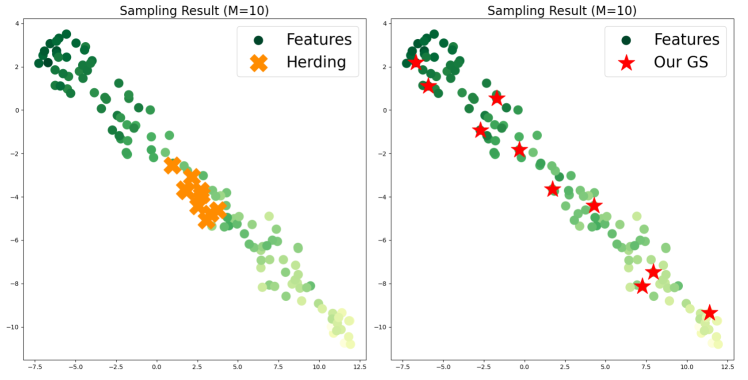
Figure 5: T-SNE Visualizations of the features sampled by Herding (left) and our GS (right) after training on the first task. Points in greens denotes the features. Darker color indicates higher score. Points in orange and red denote the feature sampled by Herding and our GS, respectively. The exemplars sampled by our GS can cover all score levels and roughly describe the learned feature distribution rather than gathering in a compact region. Best viewed in color.

TABLE V: Ablation studies about the proposed rehearsal-based paradigm on the AQA-7 dataset. We design three other possible substitutes for comparisons. A variant named “xx-Aug-yy” indicates we adopt “xx” (No Augmentation / F-Aug / FS-Aug) to augment features and utilize “yy” (A-Rgs / A-Diff / A-Dist) to constrain the forgetting.

Variants	F-Aug	FS-Aug	A-Rgs	A-Diff	A-Dist	$\mathcal{AP}(\uparrow)$	$\mathcal{NBT}(\downarrow)$	$\mathcal{MF}(\downarrow)$
No-Aug-Dist					✓	0.6261	0.1292	0.1606
F-Aug-Rgs	✓		✓			0.6127	0.1223	0.1532
FS-Aug-Rgs		✓	✓			0.6284	0.1197	0.1447
Ours		✓		✓		0.6492	0.1085	0.1399

- Effectiveness of Grouping Sampling. In our work, the proposed rehearsal-based method is based on the Grouping Sampling strategy. Note that lots of methods [24, 19, 41] directly adopt the Herding strategy [16] to sample representative exemplars. We conduct a comparison among Herding, Random Sampling (RS) and our Grouping Sampling (GS) under two different memory sizes, i.e., 30 and 60. As shown in Table IV, Herding gets the worst results, even worse than Random Sampling, and our GS strategy outperforms other methods regardless of the memory size. The results suggest that Herding cannot select the most representative exemplars under Continual-AQA settings. The visualization results shown in Figure 5 also support this view. The features sampled by Herding are gathered in a compact region in the latent space. The exemplars’ corresponding scores are pretty close, which cannot honestly describe the previously learned feature distribution. On the contrary, our GS, which selects representative exemplars to roughly describe the previously learned feature distribution, can serve as a general sampling strategy for Continual-AQA.

- Impact of Feature-Score co-Augmentation and Difference Loss. The Feature-Score co-Augmentation (FS-Aug) is proposed to augment features and their corresponding scores. Based on FS-Aug, an auxiliary difference loss (A-Diff) is utilized to constrain the shift of already learned feature distribution. Hence, it is worth studying if it is necessary to couple FS-Aug and A-Diff. To the end, we consider three other possible methods here:

• Feature Augmentation only (F-Aug). As a substitute for FS-Aug, following PASS [18], we augment $f^{t-1}_{pre}$ by adding random Gaussian noises without augmenting their corresponding scores.

• Auxiliary Distillation Loss (A-Dist). As a substitute for A-Diff, we directly conduct an extra feature distillation loss on $f^{t}_{pre}$ and $f^{t-1}_{pre}$.

• Auxiliary Score Regression Loss (A-Rgs). As a substitute for A-Diff, we perform an extra regression to the scores of the augmented features and adopt an auxiliary regression loss to optimize the model.

After that, we combine these methods to build and examine three other variants. As shown in Table V, our approach outperforms other possible strategies on all three metrics. The comparison between “No-Aug-Dist” and our method indicates that an auxiliary distillation loss is ineffective for mitigating forgetting. Moreover, compared with “F-Aug-Rgs”, “FS-Aug-Rgs” performs all the way better, which proves that augmenting corresponding scores together with features is necessary for Continual-AQA.

Moreover, we study the impact of the number of helpers. As shown in Figure 6, the performance improves when the number of helpers grows from 3 to 7. However, the performance is relatively poor when further increasing the number of helpers from 7 to 9. It suggests that when we set an extremely low value to the number of helpers, the augmentation direction obtained by the helpers may not be reliable enough. When an extremely high value is set to be the number of helpers, the impact of each helper tends to be offset due to the opposite direction of the perturbations.

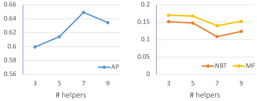
Figure 6: The impact of the number of helpers to the Average Performance(AP) and to the Negative Backward Transfer and Maximum Forgetting(NBT and MF) on the AQA-7 dataset. The X-axis indicates the number of helpers(# helpers) and the Y-axis indicates the value of the metrics.

TABLE VI: Ablation studies of the initialization for Action-specific Graph and the reformulated feature distillation loss on the AQA-7 dataset.

Variants	$\mathcal{AP}(\uparrow)$	$\mathcal{NBT}(\downarrow)$	$\mathcal{MF}(\downarrow)$
Zero-init	0.6360	0.1565	0.1803
Random-init	0.6401	0.1511	0.2068
w/ $\mathcal{L}_{FD(Naive)}$	0.6417	0.1360	0.1671
Ours	0.6492	0.1085	0.1399

V-E Analysis on Action General-Specific Graph

In our work, an Action General-Specific Graph module is developed to learn and decouple the action-general and action-specific knowledge during continual training. As introduced in Section IV-C, we utilize specific initialization for Action-Specific Graph. Moreover, we design a specific feature distillation loss to save and decouple action-general and action-specific knowledge. To demonstrate the effectiveness of such designs, on the one hand, we replace the proposed initialization with two intuitive strategies (i.e., zero initialization and random initialization). On the other hand, we replace the proposed feature distillation loss with the naive feature distillation loss in Equation 14. As shown in Table VI, when ablating any of them, the performance declines significantly, which verifies the contributions of such designs to the performance.

V-F Comparison with the Existing Methods on the AQA-7 dataset

TABLE VII: Comparisons of our approach with existing AQA methods on the AQA-7 dataset. “w/ Our GS” denotes our Grouping Sampling is adopted to sample the exemplars. “w/ PODLoss” denotes the model is trianed together with the POD Loss [24]. USDL* indicates that we frozen the I3D backbone when training USDL model.

Methods	$\mathcal{AP}(\uparrow)$	$\mathcal{NBT}(\downarrow)$	$\mathcal{MF}(\downarrow)$
AQA model + Finetuning
USDL*[25]	0.2868	0.4612	0.5573
USDL[25]	0.3344	0.5124	0.7373
CoRe-GART[21]	0.3015	0.5570	0.6336
JRG[4]	0.5523	0.2515	0.3420
AQA model + Continual Learning
USDL*[25] w/ Our GS	0.4463	0.2844	0.3621
USDL[25] w/ Our GS	0.5852	0.2364	0.3891
CoRe-GART[21] w/ Our GS	0.4716	0.3508	0.5391
CoRe-GART[21] w/ PODLoss[24] w/ Our GS	0.4956	0.3410	0.5108
Ours	0.6492	0.1085	0.1399

TABLE VIII: Comparisons of our approach with existing CL methods on the AQA-7 dataset. “w/ Our GS” denotes our Grouping Sampling is adopted to sample the exemplars.

Methods	$\mathcal{AP}(\uparrow)$	$\mathcal{NBT}(\downarrow)$	$\mathcal{MF}(\downarrow)$
Finetune	0.5523	0.2515	0.3420
Upper Bound	0.7344	-	-
Train without Memory
EWC [22]	0.5616	0.2734	0.4018
Train with Herding
iCaRL [16]	0.5811	0.2215	0.3289
PODNet [24]	0.5914	0.1989	0.2530
AFC [23]	0.5787	0.1925	0.2647
Train with Our GS
PODNet [24] w/ Our GS	0.6393	0.1371	0.1987
AFC [23] w/ Our GS	0.6489	0.1275	0.1806
Ours	0.6492	0.1085	0.1399

TABLE IX: Comparison results with various total memory sizes (M) on the AQA-7 dataset. “w/ Our GS” indicates our Grouping Sampling is adopted to sample the exemplars.

Methods	M	$\mathcal{AP}(\uparrow)$	$\mathcal{NBT}(\downarrow)$	$\mathcal{MF}(\downarrow)$
Finetune	-	0.5523	0.2515	0.3420
Upper Bound	-	0.7344	-	-
iCaRL [16]	15	0.5602	0.2323	0.3326
PODNet [24]	15	0.5789	0.1796	0.2699
PODNet [24] w/ Our GS	15	0.6013	0.1743	0.2223
Ours	15	0.6167	0.1272	0.1662
iCaRL [16]	30	0.5811	0.2215	0.3289
PODNet [24]	30	0.5914	0.1989	0.2530
PODNet [24] w/ Our GS	30	0.6393	0.1371	0.1987
Ours	30	0.6492	0.1085	0.1399
iCaRL [16]	60	0.5915	0.2068	0.2601
PODNet [24]	60	0.6012	0.1603	0.2259
PODNet [24] w/ Our GS	60	0.6621	0.1161	0.1635
Ours	60	0.6712	0.0944	0.1367

We compare the proposed method with the existing methods on the AQA-7 dataset in the following three aspects:

- Comparison with existing AQA methods. We build Cl baselines based on successful AQA models (i.e., USDL[25], CoRe-GART[21]) and compare them with our approach. The comparison results are shown in Table VII, and we have the following observations. First, when directly fine-tuning models across tasks, each method performs poorly with high forgetting. Second, we train USDL and CoRe-GART to build stronger baselines with the POD loss [24] and our GS. However, although POD loss and GS significantly improve the performance of USDL and CoRe-GART, our approach outperforms these two methods.

It is worthwhile noting that the enormous contrast in performance of USDL and CoRe-GART on conventional AQA tasks [25, 21] and Continual-AQA may lie in the great task-specific knowledge learning ability with the special problem formulations (e.g., Uncertain Distribution Prediction and Contrastive Regression). The more effective to learn specific task, the more easy to forget the already learned knowledge.

- Comparison with existing CL methods. We compare the proposed method with four existing CL methods (i.e, EWC[22], icarl[16], podnet[24], and AFC[23]). As shown in Table VIII, our method bridges the gap between “Finetune” and “Upper Bound” on $\mathcal{AP}$ and significantly alleviates forgetting. Additionally, our method outperforms other methods among the three metrics. It has been discussed in Section V-D that Herding may not be an appropriate sampling strategy for Continual-AQA. Hence, we further adopt our Grouping Sampling on PODNet and AFC for better comparison. As shown in Table VIII, when our Grouping Sampling is adopted, existing CL methods can perform better but still underperform our approach, further showing our approach’s effectiveness.

- Robustness study on memory size. We further evaluate the robustness of our approach by adjusting the total memory size (M). As shown in Table IX, our approach outperforms PODNet [24] regardless of the memory size, even if our GS is adopted.

Moreover, although increasing the memory size can stably improve the performance, there is still an explicit gap between our approach and the joint training upper bound, even if the memory size is set as 60. Such results indicate that there is still room for further research on Continual-AQA.

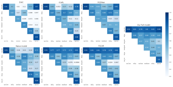
Figure 7: Visualizations of the performance matrix $P$ learned by EWC [22], iCaRL [16], PODNet [24], our naive model, our GS, our FSCAR and our full model on AQA-7 dataset. The i-row-j-column element of $P$ denotes the Spearman’s rank correlation coefficient on the $i$-th task after learning the $j$-th task. Darker color indicates better performance. The task sequence is: Sync.10m, Skiing, Gym vault, Snowboard, Diving, Sync.3m.

TABLE X: Comparisons of our approach with existing Continual Learning methods on the BEST dataset. “w/ Our GS” indicates our Grouping Sampling is adopted to sample the exemplars.

Methods	$\mathcal{AP}(\uparrow)$	$\mathcal{NBT}(\downarrow)$	$\mathcal{MF}(\downarrow)$
Finetune	0.6614	0.1976	0.2381
Upper Bound	0.8163	-	-
Train without memory
EWC [22]	0.6752	0.1856	0.2137
Train with Herding
iCaRL [16]	0.7255	0.1161	0.1378
PODNet [24]	0.7449	0.0649	0.0699
AFC [23]	0.7566	0.0535	0.0765
Train with Our GS
PODNet [24] w/ Our GS	0.7600	0.0495	0.0708
AFC [23] w/ Our GS	0.7643	0.0426	0.0542
Ours	0.7883	0.0288	0.0366

TABLE XI: Comparisons of our approach with existing Continual Learning methods on the MTL-AQA dataset. “w/ Our GS” indicates our Grouping Sampling is adopted to sample the exemplars.

Methods	$\mathcal{AP}(\uparrow)$	$\mathcal{NBT}(\downarrow)$
Finetune	0.7045	0.1697
Upper Bound	0.8260	-
Train without memory
EWC [22]	0.7198	0.1607
Train with Herding
iCaRL [16]	0.7465	0.1165
AFC [23]	0.7487	0.0979
Train with Our GS
AFC [23] w/ Our GS	0.7690	0.0624
Ours	0.7895	0.0574

V-G Comparison results on the BEST and MTL-AQA datasets

To study the versatility of our method, we conduct comparisons on two other popular AQA datasets (i.e., BEST [12] and MTL-AQA [26]) As shown in Table X and Table XI, we have the same observation as experiments on the AQA-7 dataset: our method outperforms other CL baselines on all metrics. Such results demonstrate that our method can adapt to the pairwise ranking scenario and works well in the scenario where continually learned tasks are pretty similar to the already learned ones.

V-H Intuitive Visualizations

To further show the effectiveness of our model more intuitively, we visualize the performance matrix $P$, which has been introduced in Section V-A. As shown in Figure 7, EWC [22] suffers from serious forgetting. iCaRL [16] mitigates the forgetting on the $2$-nd and $4$-th task, but preforms poorly on other tasks. PODNet [24] outperforms iCaRL [16] but still forgets a lot on the $2$-nd task. Our approach achieves the best performance with the least forgetting. Moreover, the model achieves better performance when gradually adding the proposed components.

VI Conclusions and Discussions

We conduct a work on continual learning in AQA, which has never been explored before. We claim that the key to addressing Continual-AQA is sequentially learning a task-consistent score-discriminative feature distribution across all seen tasks. To address this, we try to mitigate forgetting in Continual-AQA in two aspects. First, we propose a Feature-Score Correlation-Aware Rehearsal, which stores and reuses data from previous tasks with limited memory size, considering the relationship between latent features and action quality scores. Besides, to address the second question, an Action General-Specific Graph module is proposed to learn and decouple action-general and action-specific knowledge so that forgetting can be further mitigated.

The extensive experiments verified the effectiveness and versatility of the proposed approach. Although significant improvement has been achieved by our approach, Continual-AQA is still desirable to explore for the following reasons. First, the performance gap between our approach and the joint training upper bound is still explicit even when using a nontrivial memory size. Second, in this work, we just develop our solution based on the Directly Regression formulation of AQA (i.e., using a regressor to regress the action quality score directly). However, successful AQA models based on other formulations(e.g., Contrastive Regression [21], and Distribution Prediction [25]) are much easier to forget previously learned knowledge.

We believe the introduction of Continual-AQA and our exploration can provide a new perspective and solution for the practical application of AQA.

Algorithm 1 Training our model on a current task $t$ ($t>1$)

1:Previous feature extractor $E^{t-1}$; Previous score regressor $R^{t-1}_{s}$; Difference regressor $R^{t-1}_{d}$; Action-Specific Graph $S^{t}$ for task $t$; Current data $D^{t}$; Saved previous data $\psi=\{\psi^{1},...,\psi^{t-1}\}$; Hyper-parameters $\lambda_{FD},\lambda_{Diff},M$.

2:$E^{t},R^{t}_{s},R^{t}_{d},\psi$

3:$\text{Initialization: }E^{t},R^{t}_{s},R^{t}_{d}\leftarrow E^{t-1},R^{t-1}_{s},R^{t-1}_{d}$

4:$E^{t}\leftarrow E^{t}\cup S^{t}$

5:while until required iterations do

6:     $D^{t}_{tr}\leftarrow\textnormal{Sample a mini-batch from }D_{t}$

7:     $\mathcal{L}_{Diff},\mathcal{L}_{FD},\mathcal{L}_{AQA},N_{tr}\leftarrow 0$

8:     for $(v^{t}_{cur,i},s_{cur,i})\text{ in }D^{t}_{tr}$ do

9:         $(v^{\tau}_{pre,j},s_{pre,j})\leftarrow\text{RandomSample}(\psi)$ $\triangleright$ Randomly sample previous data. $\tau$ indicates the task id

10:         $\{(v^{\epsilon_{k}}_{hlp,k},s_{hlp,k})\}^{K}_{k=1}\leftarrow\text{RandomSample}(\psi)$ $\triangleright$ Randomly sample K augmentation helpers

11:         $\{f^{t,n}_{cur,i}\}^{t}_{n=1}\leftarrow\{E^{t}_{n}(v^{t}_{cur,i})\}^{t}_{n=1}$ $\triangleright$ Fed the current data into $E^{t}$

12:         $\{f^{t-1,n}_{cur,i}\}^{t-1}_{n=1}\leftarrow\{E^{t-1}_{n}(v^{t}_{cur,i})\}^{t-1}_{n=1}$ $\triangleright$ Fed the current data into $E^{t-1}$

13:         $\{f^{t,n}_{pre,j}\}^{t-1}_{n=1}\leftarrow\{E^{t}_{n}(v^{\tau}_{pre,j})\}^{t-1}_{n=1}$ $\triangleright$ Fed the previous data into $E^{t}$

14:         $\{f^{t-1,n}_{pre,j}\}^{t-1}_{n=1}\leftarrow\{E_{n}^{t-1}(v^{\tau}_{pre,j})\}^{t-1}_{n=1}$ $\triangleright$ Fed the previous data into $E^{t-1}$

15:         $\{f^{t-1,{\epsilon_{k}}}_{hlp,k}\}^{K}_{k=1}\leftarrow\{E^{t-1}_{\epsilon_{k}}(v^{\epsilon_{k}}_{hlp,k})\}^{K}_{k=1}$ $\triangleright$ Fed the augmentation helpers into $E^{t-1}$

16:         $(\tilde{f}^{t-1}_{pre,j},\tilde{s}_{pre,j})\leftarrow\text{FS-Aug}((f^{t-1}_{pre,j},s_{pre,j}),\{(f^{t-1}_{hlp,k},s_{hlp,k})\}^{K}_{k=1})$ $\triangleright$ Feature-Score co-Augmentation

17:         $\hat{s}_{pre,j},\hat{s}_{cur,i}\leftarrow R^{t}_{s}(f^{t,\tau}_{pre,j}),R^{t}_{s}(f^{t,t}_{cur,i})$ $\triangleright$ Computer predicted scores

18:         $d\leftarrow\tilde{s}_{pre,j}-s_{pre,j}$ $\triangleright$ Computer GT score difference via Eq. 5

19:         $\mathcal{L}_{Diff}\leftarrow\mathcal{L}_{Diff}+(R^{t}_{d}(\tilde{f}^{t-1}_{pre,j}\copyright f_{pre,j}^{t})-d)^{2}$ $\triangleright$ Compute $\mathcal{L}_{Diff}$ via Eq. 6

20:         $\mathcal{L}_{FD}\leftarrow\mathcal{L}_{FD}+\sum^{t-1}_{n=1}[||f^{t,n}_{cur,i}-f^{t-1,n}_{cur,i}||^{2}+||f^{t,n}_{pre,j}-f^{t-1,n}_{pre,j}||^{2}]/2$ $\triangleright$ Compute $\mathcal{L}_{FD}$ via Eq. 8

21:         $\mathcal{L}_{AQA}\leftarrow\mathcal{L}_{AQA}+((\hat{s}_{pre,j}-s_{pre,j})^{2}+(\hat{s}_{cur,i}-s_{cur,i})^{2})/{2}$ $\triangleright$ Compute $\mathcal{L}_{AQA}$ via MSE loss

22:         $N_{tr}\leftarrow N_{tr}+1$

23:     end for

24:     $\mathcal{L}_{Diff},\mathcal{L}_{FD},\mathcal{L}_{AQA}\leftarrow{\mathcal{L}_{Diff}}/{N_{tr}},{\mathcal{L}_{FD}}/{N_{tr}},{\mathcal{L}_{AQA}}/{N_{tr}}$

25:     $\mathcal{L}\leftarrow\mathcal{L}_{AQA}+\lambda_{FD}\mathcal{L}_{FD}+\lambda_{Diff}\mathcal{L}_{Diff}$

26:     $\text{Update }E^{t},R^{t}_{s},R^{t}_{d}\text{ by back-propagation}$

27:end while

28:$\psi\leftarrow\text{GS-Reconstruction}(\psi,M,D^{t})$ $\triangleright$ Reconstruct $\psi$ via GS

References

- [1] J. Carreira and A. Zisserman, “Quo vadis, action recognition? a new model and the kinetics dataset,” in Proceedings of the IEEE Conference on Computer Vision and Pattern Recognition, 2017, pp. 6299–6308.
- [2] C. Feichtenhofer, H. Fan, J. Malik, and K. He, “Slowfast networks for video recognition,” in Proceedings of the IEEE/CVF International Conference on Computer Vision, 2019, pp. 6202–6211.
- [3] G. Bertasius, H. Wang, and L. Torresani, “Is space-time attention all you need for video understanding?” in International Conference on Machine Learning, vol. 2, no. 3, 2021, p. 4.
- [4] J.-H. Pan, J. Gao, and W.-S. Zheng, “Action assessment by joint relation graphs,” in Proceedings of the IEEE/CVF International Conference on Computer Vision, 2019, pp. 6331–6340.
- [5] J. Xu, Y. Rao, X. Yu, G. Chen, J. Zhou, and J. Lu, “Finediving: A fine-grained dataset for procedure-aware action quality assessment,” in Proceedings of the IEEE/CVF Conference on Computer Vision and Pattern Recognition, 2022, pp. 2949–2958.
- [6] A. Xu, L.-A. Zeng, and W.-S. Zheng, “Likert scoring with grade decoupling for long-term action assessment,” in Proceedings of the IEEE/CVF Conference on Computer Vision and Pattern Recognition, 2022, pp. 3232–3241.
- [7] L.-A. Zeng, F.-T. Hong, W.-S. Zheng, Q.-Z. Yu, W. Zeng, Y.-W. Wang, and J.-H. Lai, “Hybrid dynamic-static context-aware attention network for action assessment in long videos,” in Proceedings of the 28th ACM International Conference on Multimedia, 2020, pp. 2526–2534.
- [8] Z. Li, L. Gu, W. Wang, R. Nakamura, and Y. Sato, “Surgical skill assessment via video semantic aggregation,” in International Conference on Medical Image Computing and Computer-Assisted Intervention. Springer, 2022, pp. 410–420.
- [9] D. Liu, Q. Li, T. Jiang, Y. Wang, R. Miao, F. Shan, and Z. Li, “Towards unified surgical skill assessment,” in Proceedings of the IEEE/CVF Conference on Computer Vision and Pattern Recognition, 2021, pp. 9522–9531.
- [10] A. Malpani, S. S. Vedula, C. C. G. Chen, and G. D. Hager, “Pairwise comparison-based objective score for automated skill assessment of segments in a surgical task,” in International Conference on Information Processing in Computer-Assisted Interventions. Springer, 2014, pp. 138–147.
- [11] H. Doughty, D. Damen, and W. Mayol-Cuevas, “Who’s better? who’s best? pairwise deep ranking for skill determination,” in Proceedings of the IEEE Conference on Computer Vision and Pattern Recognition, 2018, pp. 6057–6066.
- [12] H. Doughty, W. Mayol-Cuevas, and D. Damen, “The pros and cons: Rank-aware temporal attention for skill determination in long videos,” in Proceedings of the IEEE/CVF Conference on Computer Vision and Pattern Recognition, 2019, pp. 7862–7871.
- [13] R. M. French, “Catastrophic forgetting in connectionist networks,” Trends in cognitive sciences, vol. 3, no. 4, pp. 128–135, 1999.
- [14] M. McCloskey and N. J. Cohen, “Catastrophic interference in connectionist networks: The sequential learning problem,” in Psychology of Learning and Motivation. Elsevier, 1989, vol. 24, pp. 109–165.
- [15] I. J. Goodfellow, M. Mirza, D. Xiao, A. Courville, and Y. Bengio, “An empirical investigation of catastrophic forgetting in gradient-based neural networks,” arXiv preprint arXiv:1312.6211, 2013.
- [16] S.-A. Rebuffi, A. Kolesnikov, G. Sperl, and C. H. Lampert, “icarl: Incremental classifier and representation learning,” in Proceedings of the IEEE Conference on Computer Vision and Pattern Recognition, 2017, pp. 2001–2010.
- [17] S. Ebrahimi, F. Meier, R. Calandra, T. Darrell, and M. Rohrbach, “Adversarial continual learning,” in European Conference on Computer Vision. Springer, 2020, pp. 386–402.
- [18] F. Zhu, X.-Y. Zhang, C. Wang, F. Yin, and C.-L. Liu, “Prototype augmentation and self-supervision for incremental learning,” in Proceedings of the IEEE/CVF Conference on Computer Vision and Pattern Recognition, 2021, pp. 5871–5880.
- [19] Y. Wu, Y. Chen, L. Wang, Y. Ye, Z. Liu, Y. Guo, and Y. Fu, “Large scale incremental learning,” in Proceedings of the IEEE/CVF Conference on Computer Vision and Pattern Recognition, 2019, pp. 374–382.
- [20] S. Hou, X. Pan, C. C. Loy, Z. Wang, and D. Lin, “Learning a unified classifier incrementally via rebalancing,” in Proceedings of the IEEE/CVF Conference on Computer Vision and Pattern Recognition, 2019, pp. 831–839.
- [21] X. Yu, Y. Rao, W. Zhao, J. Lu, and J. Zhou, “Group-aware contrastive regression for action quality assessment,” in Proceedings of the IEEE/CVF International Conference on Computer Vision, 2021, pp. 7919–7928.
- [22] J. Kirkpatrick, R. Pascanu, N. Rabinowitz, J. Veness, G. Desjardins, A. A. Rusu, K. Milan, J. Quan, T. Ramalho, A. Grabska-Barwinska et al., “Overcoming catastrophic forgetting in neural networks,” Proceedings of the National Academy of Sciences, vol. 114, no. 13, pp. 3521–3526, 2017.
- [23] M. Kang, J. Park, and B. Han, “Class-incremental learning by knowledge distillation with adaptive feature consolidation,” in Proceedings of the IEEE/CVF Conference on Computer Vision and Pattern Recognition, 2022, pp. 16 071–16 080.
- [24] A. Douillard, M. Cord, C. Ollion, T. Robert, and E. Valle, “Podnet: Pooled outputs distillation for small-tasks incremental learning,” in European Conference on Computer Vision. Springer, 2020, pp. 86–102.
- [25] Y. Tang, Z. Ni, J. Zhou, D. Zhang, J. Lu, Y. Wu, and J. Zhou, “Uncertainty-aware score distribution learning for action quality assessment,” in Proceedings of the IEEE/CVF Conference on Computer Vision and Pattern Recognition, 2020, pp. 9839–9848.
- [26] P. Parmar and B. T. Morris, “What and how well you performed? a multitask learning approach to action quality assessment,” in Proceedings of the IEEE/CVF Conference on Computer Vision and Pattern Recognition, 2019, pp. 304–313.
- [27] Y. Bai, D. Zhou, S. Zhang, J. Wang, E. Ding, Y. Guan, Y. Long, and J. Wang, “Action quality assessment with temporal parsing transformer,” in European Conference on Computer Vision. Springer, 2022, pp. 422–438.
- [28] S. Wang, D. Yang, P. Zhai, C. Chen, and L. Zhang, “Tsa-net: Tube self-attention network for action quality assessment,” in Proceedings of the 29th ACM International Conference on Multimedia, 2021, pp. 4902–4910.
- [29] K. Zhou, Y. Ma, H. P. H. Shum, and X. Liang, “Hierarchical graph convolutional networks for action quality assessment,” IEEE Transactions on Circuits and Systems for Video Technology, 2023.
- [30] C. Xu, Y. Fu, B. Zhang, Z. Chen, Y.-G. Jiang, and X. Xue, “Learning to score figure skating sport videos,” IEEE Transactions on Circuits and Systems for Video Technology, vol. 30, no. 12, pp. 4578–4590, 2020.
- [31] S.-J. Zhang, J.-H. Pan, J. Gao, and W.-S. Zheng, “Semi-supervised action quality assessment with self-supervised segment feature recovery,” IEEE Transactions on Circuits and Systems for Video Technology, 2022.
- [32] P. Parmar, A. Gharat, and H. Rhodin, “Domain knowledge-informed self-supervised representations for workout form assessment,” in Computer Vision–ECCV 2022: 17th European Conference, Tel Aviv, Israel, October 23–27, 2022, Proceedings, Part XXXVIII. Springer, 2022, pp. 105–123.
- [33] S.-J. Zhang, J.-H. Pan, J. Gao, and W.-S. Zheng, “Adaptive stage-aware assessment skill transfer for skill determination,” IEEE Transactions on Multimedia, pp. 1–12, 2023.
- [34] Z. Wang, Z. Zhang, S. Ebrahimi, R. Sun, H. Zhang, C.-Y. Lee, X. Ren, G. Su, V. Perot, J. Dy et al., “Dualprompt: Complementary prompting for rehearsal-free continual learning,” arXiv preprint arXiv:2204.04799, 2022.
- [35] J.-H. Pan, J. Gao, and W.-S. Zheng, “Adaptive action assessment,” IEEE Transactions on Pattern Analysis and Machine Intelligence, 2021.
- [36] C. Xu, Y. Fu, B. Zhang, Z. Chen, Y.-G. Jiang, and X. Xue, “Learning to score figure skating sport videos,” IEEE Transactions on Circuits and Systems for Video Technology, vol. 30, no. 12, pp. 4578–4590, 2019.
- [37] Z. Li and D. Hoiem, “Learning without forgetting,” IEEE Transactions on Pattern Analysis and Machine Intelligence, vol. 40, no. 12, pp. 2935–2947, 2017.
- [38] P. Parmar and B. Morris, “Action quality assessment across multiple actions,” in 2019 IEEE Winter Conference on Applications of Computer Vision. IEEE, 2019, pp. 1468–1476.
- [39] H. Liu, K. Simonyan, and Y. Yang, “Darts: Differentiable architecture search,” arXiv preprint arXiv:1806.09055, 2018.
- [40] D. P. Kingma and J. Ba, “Adam: A method for stochastic optimization,” arXiv preprint arXiv:1412.6980, 2014.
- [41] J. Park, M. Kang, and B. Han, “Class-incremental learning for action recognition in videos,” in Proceedings of the IEEE/CVF International Conference on Computer Vision, 2021, pp. 13 698–13 707.