Obtaining Pseudo-inverse Solutions With MINRES

Abstract

The celebrated minimum residual method (MINRES), proposed in the seminal paper of Paige and Saunders [49], has seen great success and wide-spread use in solving linear least-squared problems involving Hermitian matrices, with further extensions to complex symmetric settings. Unless the system is consistent whereby the right-hand side vector lies in the range of the matrix, MINRES is not guaranteed to obtain the pseudo-inverse solution. Variants of MINRES, such as MINRES-QLP [17], which can achieve such minimum norm solutions, are known to be both computationally expensive and challenging to implement. We propose a novel and remarkably simple lifting strategy that seamlessly integrates with the final MINRES iteration, enabling us to obtain the minimum norm solution with negligible additional computational costs. We study our lifting strategy in a diverse range of settings encompassing Hermitian and complex symmetric systems as well as those with semi-definite preconditioners. We also provide numerical experiments to support our analysis and showcase the effects of our lifting strategy.

1 Introduction

We consider the linear least-squares problem,

$$\min_{\mathbf{x}\in\mathbb{C}^{d}}\|\mathbf{b}-\mathbf{A}\mathbf{x}\|^{2},$$ (1)

involving a complex-valued matrix $\mathbf{A}\in\mathbb{C}^{d\times d}$ that is either Hermitian or complex symmetric, and a right-hand side complex vector $\mathbf{b}\in\mathbb{C}^{d}$. Our primary focus is on cases where the system is inconsistent, i.e., $\mathbf{b}\notin\textnormal{Range}(\mathbf{A})$, which arise in a vast variety of situations such as in optimization of non-convex problems [51, 41], numerical solution of partial differential equations [37], and low-rank matrix computations [27]. In fact, even if the system is theoretically consistent, due to errors from measurements, discretizations, truncations, or round-off, the matrix $\mathbf{A}$ can become numerically singular, resulting in a numerically incompatible system [16]. In these situations, problem 1 admits infinitely many solutions. Among all of these solutions, the one with the smallest Euclidean norm is commonly referred to as the pseudo-inverse solution, also known as the minimum-norm solution, and is given by $\mathbf{A}^{\dagger}\mathbf{b}$ where $\mathbf{A}^{\dagger}$ is the Moore-Penrose pseudo-inverse of $\mathbf{A}$. This particular solution, among all other alternatives, holds a special place and offers numerous practical and theoretical advantages in various applications including, e.g., linear matrix equations [25], optimization [51, 40], and machine learning [23, 21].

When $d$ is small, one can obtain $\mathbf{A}^{\dagger}\mathbf{b}$ by explicitly computing $\mathbf{A}^{\dagger}$ via direct methods, e.g., [20, 38, 12, 11, 39]. Among them, the most well-known direct method to obtain $\mathbf{A}^{\dagger}$ is via the singular value decomposition [39]. However, rather than explicitly computing $\mathbf{A}^{\dagger}$ for large-scale problems when $d\gg 1$, it is more appropriate, if not indispensable, to obtain the pseudo-inverse solution $\mathbf{A}^{\dagger}\mathbf{b}$ by an iterative scheme. LSQR [50] and LSMR [26] are iterative Krylov sub-space methods that can recover the pseudo-inverse solution $\mathbf{A}^{\dagger}\mathbf{b}$ for any $\mathbf{A}\in\mathbb{C}^{m\times d}$. However, they are mathematically equivalent to the conjugate gradient method (CG) [33] and the minimum residual method (MINRES) [49], respectively, applied to the normal equation of 1. Consequently, each iteration of LSQR and LSMR necessitates two matrix-vector product evaluations, which can be computationally challenging when $d\gg 1$. While CG iterations are not well-defined unless $\mathbf{A}\succeq\mathbf{0}$ and $\mathbf{b}\in\textnormal{Range}(\mathbf{A})$, MINRES can effectively solve 1 even for indefinite systems. Nonetheless, MINRES is not guaranteed to obtain $\mathbf{A}^{\dagger}\mathbf{b}$ unless $\mathbf{b}\in\textnormal{Range}(\mathbf{A})$ [17, Theorem 3.1]. To address this limitation, a variant of MINRES, called MINRES-QLP was introduced in [17, 18]. MINRES-QLP ensures convergence to the pseudo-inverse solution in all cases. Compared with MINRES, the rank-revealing QLP decomposition of the tridiagonal matrix from the Lanczos process in MINRES-QLP necessitates additional computations per iteration [17]. Moreover, owing to its increased complexity, the implementation of MINRES-QLP can pose greater challenges than that of MINRES.

In this paper, we introduce a novel and remarkably simple strategy that seamlessly incorporates into the final MINRES iteration, allowing us to obtain the minimum norm solution with negligible additional computational overhead and minimal alterations to the original MINRES algorithm. We consider our lifting strategy in a variety of settings including Hermitian and complex symmetric systems as well as systems with semi-definite preconditioners.

The rest of the paper is organized as follows. We end this section by introducing our notation and definitions. The theoretical analyses underpinning our lifting strategy in a variety of settings are given in Sections 2 and 3. In particular, Sections 2.1 and 2.2 consider Hermitian and complex symmetric systems, respectively, while Sections 3.1 and 3.2 study our lifting strategy in the presence of positive semi-definite preconditioners in each matrix class. Numerical results are given in Section 4. Conclusion and further thoughts are gathered in Section 5.

Notation and Definition

Throughout the paper, vectors and matrices are denoted by bold lower- and upper-case letters, respectively. Regular lower-case letters are reserved for scalars. The space of complex-symmetric and Hermitian $d\times d$ matrices are denoted by $\mathbb{S}^{d\times d}$ and $\mathbb{H}^{d\times d}$, respectively. The inner-product of complex vectors $\mathbf{x}$ and $\mathbf{y}$ is defined as $\langle\mathbf{x},\mathbf{y}\rangle=\mathbf{x}^{*}\mathbf{y}$, where $\mathbf{x}^{*}$ represents the conjugate transpose of $\mathbf{x}$. The Euclidean norm of a vector $\mathbf{x}\in\mathbb{C}^{d}$ is given by $\|\mathbf{x}\|$. The conjugate of a vector or a matrix is denoted by $\bar{\mathbf{b}}=\textnormal{Conj}(\mathbf{b})$ or $\bar{\mathbf{A}}=\textnormal{Conj}(\mathbf{A})$. The zero vector and the zero matrix are denoted by $\mathbf{0}$ while the identity matrix of dimension $t\times t$ is given by $\mathbf{I}_{t}$. We use $\mathbf{e}_{j}$ to denote the $j\textsuperscript{th}$ column of the identity matrix. We use $\mathbf{M}\succeq\,(\succ)\,\mathbf{0}$, to indicate that $\mathbf{M}$ is positive semi-definite (PSD) (positive definite (PD)). For a PSD matrix $\mathbf{M}$, we write $\|\mathbf{x}\|_{\mathbf{M}}=\sqrt{\langle\mathbf{x},\mathbf{M}\mathbf{x}\rangle}$ (this is an abuse of notation since unless $\mathbf{M}\succ\mathbf{0}$, this does not imply a norm). For any $t\geq 1$, the set $\mathcal{K}_{t}(\mathbf{A},\mathbf{b})=\textnormal{Span}\left\{\mathbf{b},\mathbf{A}\mathbf{b},\ldots,\mathbf{A}^{t-1}\mathbf{b}\right\}$ denotes the Krylov sub-space of degree $t$ generated using $\mathbf{A}$ and $\mathbf{b}$. The residual vector at $t\textsuperscript{th}$ iteration is denoted by $\mathbf{r}_{t}=\mathbf{b}-\mathbf{A}\mathbf{x}_{t}$.

Recall the definition of the Moore-Penrose pseudo-inverse of $\mathbf{A}$. For given $\mathbf{A}\in\mathbb{C}^{d\times m}$, the (Moore-Penrose) pseudo-inverse is the matrix $\mathbf{B}\in\mathbb{C}^{m\times d}$ satisfying the Moore-Penrose conditions, namely

$$\mathbf{A}\mathbf{B}\mathbf{A} =\mathbf{A},$$ (2a)

$$\mathbf{B}\mathbf{A}\mathbf{B} =\mathbf{B},$$ (2b)

$$(\mathbf{A}\mathbf{B})^{*} =\mathbf{A}\mathbf{B},$$ (2c)

$$(\mathbf{B}\mathbf{A})^{*} =\mathbf{B}\mathbf{A}.$$ (2d)

The matrix $\mathbf{B}$ is unique and is denoted by $\mathbf{A}^{\dagger}$. The point $\mathbf{x}^{+}\triangleq\mathbf{A}^{\dagger}\mathbf{b}$ is said to be the (Moore-Penrose) pseudo-inverse solution of 1.

The interplay between $\mathbf{A}$ and $\mathbf{b}$ is a critical factor in the convergence of MINRES and many other iterative solvers. This interplay is encapsulated in the notion of the grade of $\mathbf{b}$ with respect to $\mathbf{A}$.

The grade of $\mathbf{b}\in\mathbb{C}^{d}$ with respect to $\mathbf{A}\in\mathbb{C}^{d\times d}$ is the positive integer $g(\mathbf{A},\mathbf{b})$ such that $\text{dim}(\mathcal{K}_{t}(\mathbf{A},\mathbf{b}))=\min\{t,g(\mathbf{A},\mathbf{b})\}$. In the special case where $\mathbf{A}$ is complex-symmetric, i.e., $\mathbf{A}^{\intercal}=\mathbf{A}$, we define the grade $g(\mathbf{A},\mathbf{b})$ with respect to a modified Krylov subspace, the so-called Saunders subspaces, cf. [16, 55] and (6), i.e., $\text{dim}(\mathcal{S}_{t}(\mathbf{A},\mathbf{b}))=\min\{t,g(\mathbf{A},\mathbf{b})\}$. Recall that $g(\mathbf{A},\mathbf{b})$, in fact, determines the iteration at which a Kryolov subspace algorithm terminates with a solution (in exact arithmetic). For simplicity, for given pairs $(\mathbf{A},\mathbf{b})$ and $(\tilde{\mathbf{A}},\tilde{\mathbf{b}})$, we set $g=g(\mathbf{A},\mathbf{b})$ and $\tilde{g}=g(\tilde{\mathbf{A}},\tilde{\mathbf{b}})$.

2 Pseudo-inverse Solutions in MINRES

The most common method to compute the pseudo-inverse of a matrix is via singular value decomposition (SVD). The computational cost of the SVD is $\mathcal{O}(d^{3})$, which essentially makes such an approach intractable in high-dimensions. In our context, we do not seek to directly compute $\mathbf{A}^{\dagger}$ as our interest lies only in obtaining the pseudo-inverse solution, i.e., $\mathbf{x}^{+}=\mathbf{A}^{\dagger}\mathbf{b}$. As alluded to earlier in Section 1, existing iterative methods that can ensure the pseudo-inverse solution of 1 in the incompatible setting demand significantly higher computational effort per iteration compared to plain MINRES.

The MINRES method is shown in Algorithm 1. Recall that for a Hermitian matrix $\mathbf{A}\in\mathbb{H}^{d\times d}$ and a right-hand side vector $\mathbf{b}\in\mathbb{C}^{d}$, the $t\textsuperscript{th}$ iteration of MINRES for solving 1 can be written as

$$\min_{\mathbf{x}\in\mathcal{K}_{t}(\mathbf{A},\mathbf{b})}\|\mathbf{b}-\mathbf{A}\mathbf{x}\|^{2},$$ (3)

where $t\leq g$ and the grade $g$ is defined as in Section 1; see [49, 42] for more details. When $\mathbf{b}\in\textnormal{Range}(\mathbf{A})$, it can be easily shown that MINRES returns the pseudo-inverse solution of 1, [17]. However, when $\mathbf{b}\notin\textnormal{Range}(\mathbf{A})$, the situation is more complicated. In such settings, as long as $\textnormal{Range}(\mathbf{A})\subseteq\mathcal{K}_{g}(\mathbf{A},\mathbf{b})$, the final iterate of MINRES satisfies the properties 2a, 2b and 2c in Section 1, otherwise one can only guarantee 2b and 2c; see, e.g., [15, Theorem 2.27]. To obtain a solution that satisfies all four properties of the pseudo-inverse, Choi et al., [17], provide an algorithm, called MINRES-QLP. However, not only is MINRES-QLP rather complicated to implement, but it also demands more computations per iteration compared to MINRES.

Our goal in this section is to obtain the pseudo-inverse solution of 1 with minimal additional costs and alterations to the MINRES algorithm. Before doing so, we first restate a simple and well-known result for solutions of the least squares problem 1; the proof of Lemma 2 can be found in, e.g., [11]. The vector $\mathbf{x}$ is a solution of 1 if and only if there exists a vector $\mathbf{y}\in\mathbb{C}^{d}$ such that $\mathbf{x}=\mathbf{A}^{\dagger}\mathbf{b}+(\mathbf{I}_{d}-\mathbf{A}^{\dagger}\mathbf{A})\mathbf{y}$. Furthermore, for any solution $\mathbf{x}$, we have $\mathbf{A}\mathbf{x}=\mathbf{A}\mathbf{A}^{\dagger}\mathbf{b}$ and $\mathbf{r}=\mathbf{b}-\mathbf{A}\mathbf{x}=(\mathbf{I}-\mathbf{A}\mathbf{A}^{\dagger})\mathbf{b}$. By Section 2, the general solution of 1 is given by

$$\mathbf{x}=\mathbf{x}^{+}+\mathbf{z},\quad\text{where }\quad\mathbf{z}\in\textnormal{Null}(\mathbf{A}).$$

In other words, at $t=g$, the final iterate of MINRES is a vector that is implicitly given as a linear combination of two vectors, namely $\mathbf{A}^{\dagger}\mathbf{b}$ and some $\mathbf{z}\in\textnormal{Null}(\mathbf{A})$. Our lifting technique amounts to eliminating the component $\mathbf{z}$ to obtain the pseudo-inverse solution $\mathbf{x}^{+}$.

2.1 Hermitian and skew-Hermitian Systems

We now detail our lifting strategy to obtain the pseudo-inverse solution of 1 from MINRES iterations. We show that not only does our strategy apply to the typical case where $\mathbf{A}$ is Hermitian, but it can also be readily adapted to cases where the underlying matrix is skew-Hermitian [29].

[Lifting for Hermitian Systems] Let $\mathbf{x}_{g}$ be the final iterate of Algorithm 1 for solving 1 with the Hermitian matrix $\mathbf{A}\in\mathbb{H}^{d\times d}$.

1. If $\mathbf{r}_{g}=\bm{0}$, then $\mathbf{x}_{g}=\mathbf{A}^{\dagger}\mathbf{b}$.

2. If $\mathbf{r}_{g}\neq\bm{0}$, define the lifted vector

   $$\hat{\mathbf{x}}^{+}=\mathbf{x}_{g}-\frac{\langle\mathbf{r}_{g},\mathbf{x}_{g}\rangle}{\|\mathbf{r}_{g}\|^{2}}\mathbf{r}_{g}=\left(\mathbf{I}_{d}-\frac{\mathbf{r}_{g}\mathbf{r}_{g}^{*}}{\|\mathbf{r}_{g}\|^{2}}\right)\mathbf{x}_{g},$$ (4)

   where $\mathbf{r}_{g}=\mathbf{b}-\mathbf{A}\mathbf{x}_{g}$. Then, we have $\hat{\mathbf{x}}^{+}=\mathbf{A}^{\dagger}\mathbf{b}$.

Proof.

If $\mathbf{r}_{g}=\bm{0}$, since $\mathbf{b}\in\textnormal{Range}(\mathbf{A})$, we naturally obtain $\mathbf{x}_{g}=\mathbf{x}^{+}$ by [17, Theorem 3.1]. Now, suppose $\mathbf{r}_{g}\neq\mathbf{0}$, which implies $\mathbf{b}\not\in\textnormal{Range}(\mathbf{A})$. Since $\mathbf{x}_{g}\in\mathcal{K}_{g}(\mathbf{A},\mathbf{b})$, we can write $\mathbf{x}_{g}=\sum_{i=1}^{g}a_{i}\mathbf{A}^{i-1}\mathbf{b}$ for some $a_{i}\in\mathbb{C}$, $i=1,\dots,g$. It then follows

$$\mathbf{x}_{g}=\mathbf{x}_{g}-a_{1}(\mathbf{I}-\mathbf{A}\mathbf{A}^{\dagger})\mathbf{b}+a_{1}(\mathbf{I}-\mathbf{A}\mathbf{A}^{\dagger})\mathbf{b}=\mathbf{p}+{\mathbf{q}},$$

where

$$\mathbf{p} \triangleq\mathbf{x}_{g}-a_{1}(\mathbf{I}-\mathbf{A}\mathbf{A}^{\dagger})\mathbf{b}=a_{1}\mathbf{A}\mathbf{A}^{\dagger}\mathbf{b}+{\sum}_{i=2}^{g}a_{i}\mathbf{A}^{i-1}\mathbf{b},$$

$${\mathbf{q}} \triangleq a_{1}(\mathbf{I}-\mathbf{A}\mathbf{A}^{\dagger})\mathbf{b}=a_{1}\mathbf{r}_{g}.$$

Since $\mathbf{A}$ is Hermitian, we have $\mathbf{A}^{2}\mathbf{A}^{\dagger}=\mathbf{A}$ [9, Fact 6.3.17]. So $\mathbf{A}\mathbf{p}=\mathbf{A}\mathbf{x}_{g}$, which implies that the normal equation is satisfied for $\mathbf{p}$. In other words, $\mathbf{p}$ is a solution to 1. We also recall from Section 2 that $\mathbf{x}_{g}=\mathbf{A}^{\dagger}\mathbf{b}+\left(\mathbf{I}_{d}-\mathbf{A}^{\dagger}\mathbf{A}\right)\mathbf{y}$ for some $\mathbf{y}\in\mathbb{C}^{d}$. Now, since $\mathbf{p}\in\textnormal{Range}(\mathbf{A})=\textnormal{Range}(\mathbf{A}^{\dagger})$ and ${\mathbf{q}}\in\textnormal{Null}(\mathbf{A})$, we must have that $\mathbf{p}=\mathbf{A}^{\dagger}\mathbf{b}$. Also, since $\mathbf{p}\perp{\mathbf{q}}$, we can find $a_{1}$ as

$$a_{1}=\frac{\langle\mathbf{r}_{g},\mathbf{x}_{g}\rangle}{\|\mathbf{r}_{g}\|^{2}},$$

which gives the desired result. ∎

In Section 2.1, we relate the lifting strategy at iteration $t$ of MINRES to the orthogonal projection of the iterate ${\mathbf{x}}_{t}$ onto $\mathbf{A}\mathcal{K}_{t}(\mathbf{A},\mathbf{b})$. Consequently, performing lifting at the final iteration amounts to the orthogonal projection of $\mathbf{x}_{g}$ onto $\mathbf{A}\mathcal{K}_{g}(\mathbf{A},\mathbf{b})$, effectively eliminating the contribution of the portion of $\mathbf{b}$ that lies in the null space of $\mathbf{A}$ from the final solution. In MINRES, $\hat{\mathbf{x}}_{t}^{\natural}$ is the orthogonal projection of ${\mathbf{x}}_{t}$ onto $\mathbf{A}\mathcal{K}_{t}(\mathbf{A},\mathbf{b})$, where

$$\hat{\mathbf{x}}_{t}^{\natural}\triangleq{\mathbf{x}}_{t}-\frac{\langle{\mathbf{r}}_{t},{\mathbf{x}}_{t}\rangle}{\|{\mathbf{r}}_{t}\|^{2}}{\mathbf{r}}_{t}=\left(\mathbf{I}_{d}-\frac{{\mathbf{r}}_{t}{\mathbf{r}}_{t}^{*}}{\|{\mathbf{r}}_{t}\|^{2}}\right){\mathbf{x}}_{t}.$$ (5)

Proof.

Note that, for $t\leq g-1$, $\mathbf{A}\mathcal{K}_{t}(\mathbf{A},\mathbf{b})=\textnormal{Span}\{\mathbf{A}\mathbf{b},\mathbf{A}^{2}\mathbf{b},\ldots,\mathbf{A}^{t}\mathbf{b}\}$ is a $t$ dimensional subspace. The oblique projection framework gives ${\mathbf{r}}_{t}\perp\mathbf{A}\mathcal{K}_{t}(\mathbf{A},\mathbf{b})$. Therefore, $\mathcal{K}_{t+1}(\mathbf{A},\mathbf{b})=\textnormal{Span}\{{\mathbf{r}}_{t}\}\oplus\mathbf{A}\mathcal{K}_{t}(\mathbf{A},\mathbf{b})$ and $\mathcal{K}_{t+1}(\mathbf{A},\mathbf{b})$ has dimension $t+1$. From ${\mathbf{x}}_{t}\in\mathcal{K}_{t}(\mathbf{A},\mathbf{b})\subset\mathcal{K}_{t+1}(\mathbf{A},\mathbf{b})$, it follows that

$${\mathbf{x}}_{t}=\mathbf{P}_{{\mathbf{r}}_{t}}{\mathbf{x}}_{t}+\mathbf{P}_{\mathbf{A}\mathcal{K}_{t}}{\mathbf{x}}_{t},$$

where $\mathbf{P}_{{\mathbf{r}}_{t}}$ and $\mathbf{P}_{\mathbf{A}\mathcal{K}_{t}}$ are orthogonal projections onto the span of ${\mathbf{r}}_{t}$ and the sub-space $\mathbf{A}\mathcal{K}_{t}(\mathbf{A},\mathbf{b})$, respectively. Noting that $\mathbf{P}_{{\mathbf{r}}_{t}}={\mathbf{r}}_{t}{\mathbf{r}}_{t}^{*}/\|{\mathbf{r}}_{t}\|^{2}$ gives the desired result. ∎

Recall that if $\mathbf{A}$ is skew-Hermitian, i.e., $\mathbf{A}^{*}=-\mathbf{A}$, then we have $i\mathbf{A}\in\mathbb{H}^{d\times d}$. Thus, by [16], we can apply MINRES with inputs $i\mathbf{A}$ and $i\mathbf{b}$ to solve 3. We immediately obtain the following result. [Lifting for Skew-Hermitian Systems] If $\mathbf{A}\in\mathbb{C}^{d\times d}$ is skew-Hermitian, the result of Section 2.1 continues to hold as long as Algorithm 1 is applied with inputs $i\mathbf{A}$ and $i\mathbf{b}$. Note that, here, $\mathbf{r}_{g}=i\mathbf{b}-i\mathbf{A}\mathbf{x}_{g}$.

Proof.

We can easily verify that $-i\mathbf{A}^{\dagger}$ is the pseudo inverse of $i\mathbf{A}$ by Section 1. Hence, we obtain the desired result as in the proof of Section 2.1 by noticing $[i\mathbf{A}]^{\dagger}(i\mathbf{b})=-i\mathbf{A}^{\dagger}i\mathbf{b}=\mathbf{A}^{\dagger}\mathbf{b}$. ∎

Algorithm 1 The left column presents the MINRES algorithm for the Hermitian case, while the right column outlines the particular modifications needed for complex symmetric settings.

Hermitian Complex-symmetric

2.2 Complex-symmetric Systems

We now consider the case where $\mathbf{A}\in\mathbb{S}^{d\times d}$ is complex-symmetric, i.e., $\mathbf{A}^{\intercal}=\mathbf{A}$ but $\mathbf{A}^{*}\neq\mathbf{A}$. Least-squares systems involving such matrices arise in many applications such as data fitting [43, 2], viscoelasticity [19, 4], quantum dynamics [7, 6], electromagnetics [3], and power systems [36]. Although MINRES was initially designed for handling Hermitian systems, it has since been extended to complex-symmetric settings [16]. Here, we extend our lifting procedure for obtaining the pseudo-inverse solution in such settings.

In order to provide clear explanations for the lifting strategy in this case, we first briefly review the construction of the extension of MINRES that is adapted for complex-symmetric systems. For this, we mostly follow the development in the original work of [16] with a few modifications.

Saunders process

For complex-symmetric system, the usual Lanczos process [49] is replaced with what is referred to as the Saunders process [16, 55]. After $t$ iterations of the Saunders process, and in the absence of round-off errors, the Saunders vectors form an orthogonal matrix $\mathbf{V}_{t+1}=[\mathbf{v}_{1},\mathbf{v}_{2},\dots,\mathbf{v}_{t+1}]\in\mathbb{C}^{d\times(t+1)}$, whose columns span $\mathcal{S}_{t+1}(\mathbf{A},\mathbf{b})$ and satisfy the relation $\mathbf{A}\bar{\mathbf{V}}_{t}=\mathbf{V}_{t+1}\hat{\mathbf{T}}_{t}$. Recall that the Saunders subspace [16, 55] is defined as

$$\mathcal{S}_{t}(\mathbf{A},\mathbf{b})={\mathcal{K}_{t_{1}}}(\mathbf{A}\bar{\mathbf{A}},\mathbf{b})\oplus{\mathcal{K}_{t_{2}}}(\mathbf{A}\bar{\mathbf{A}},\mathbf{A}\bar{\mathbf{b}}),\quad t_{1}+t_{2}=t,\quad 0\leq t_{1}-t_{2}\leq 1,$$ (6)

where $\oplus$ is the direct sum operator. Here, $\hat{\mathbf{T}}_{t}$ is a tridiagonal upper-Hessenberg matrix of the form

$$\hat{\mathbf{T}}_{t} =\begin{bmatrix}\alpha_{1}&\beta_{2}&&&\\ \beta_{2}&\alpha_{2}&\beta_{3}&&\\ &\beta_{3}&\alpha_{3}&\ddots&\\ &&\ddots&\ddots&\beta_{t}\\ &&&\beta_{t}&\alpha_{t}\\ \hdashline&&&&\beta_{t+1}\\ \end{bmatrix}\triangleq\begin{bmatrix}\mathbf{T}_{t}\\ \beta_{t+1}\mathbf{e}^{\intercal}_{t}\end{bmatrix}\in\mathbb{C}^{(t+1)\times t},$$ (7)

where $\mathbf{T}_{t}^{\intercal}=\mathbf{T}_{t}=\mathbf{V}_{t}^{*}\mathbf{A}\bar{\mathbf{V}}_{t}=\mathbf{V}_{t}^{*}\mathbf{U}\mathbf{\Sigma}\mathbf{U}^{\intercal}\bar{\mathbf{V}}_{t}\in\mathbb{C}^{t\times t}$ is complex-symmetric. Subsequently, we get the three-term recursion

$$\mathbf{A}\bar{\mathbf{v}}_{t}=\beta_{t}\mathbf{v}_{t-1}+\alpha_{t}\mathbf{v}_{t}+\beta_{t+1}\mathbf{v}_{t+1},\quad t\geq 1,$$ (8)

where $\alpha_{t}$ can be computed as $\alpha_{t}=\langle\mathbf{v}_{t},\mathbf{A}\bar{\mathbf{v}}_{t}\rangle$, and $\beta_{t+1}>0$ is chosen by enforcing that $\mathbf{v}_{t+1}$ is a unit vector for all $1\leq t\leq g-1$, i.e., $\beta_{t+1}=\|\beta_{t+1}\mathbf{v}_{t+1}\|$. Letting $\mathbf{x}_{t}=\bar{\mathbf{V}}_{t}\mathbf{y}_{t}$ for some $\mathbf{y}_{t}\in\mathbb{C}^{t}$, it follows that the residual $\mathbf{r}_{t}$ can be written as

$$\mathbf{r}_{t}=\mathbf{b}-\mathbf{A}\mathbf{x}_{t}=\mathbf{b}-\mathbf{A}\bar{\mathbf{V}}_{t}\mathbf{y}_{t}=\mathbf{b}-\mathbf{V}_{t+1}\hat{\mathbf{T}}_{t}\mathbf{y}_{t}=\mathbf{V}_{t+1}(\beta_{1}\mathbf{e}_{1}-\hat{\mathbf{T}}_{t}\mathbf{y}_{t}),$$

where $\beta_{1}=\|\mathbf{b}\|$, which yields the sub-problems of complex-symmetric MINRES,

$$\min_{\mathbf{y}_{t}\in\mathbb{C}^{t}}\|\beta_{1}\mathbf{e}_{1}-\hat{\mathbf{T}}_{t}\mathbf{y}_{t}\|^{2}.$$ (9)

QR decomposition

In contrast to [16], to perform the QR decomposition of $\hat{\mathbf{T}}_{t}$, we employ the complex-symmetric Householder reflector [57, Exercise 10.4]. This is a judicious choice to maintain some of the classical properties of MINRES in the Hermitian case such as $\|{\mathbf{r}}_{t}\|=\phi_{t}>0$, as well as the singular value approximations using $\gamma_{t}^{[2]}>0$. Doing this, we obtain $\mathbf{Q}_{t}\in\mathbb{C}^{(t+1)\times(t+1)}$ and $\hat{\mathbf{R}}_{t}\in\mathbb{C}^{(t+1)\times t}$ via

$$\mathbf{Q}_{t}\hat{\mathbf{T}}_{t}=\hat{\mathbf{R}}_{t}\triangleq\begin{bmatrix}\mathbf{R}_{t}\\ \mathbf{0}^{\intercal}\end{bmatrix},\quad\mathbf{R}_{t}=\begin{bmatrix}\gamma_{1}^{[2]}&\delta_{2}^{[2]}&\epsilon_{3}&\\ &\gamma_{2}^{[2]}&\delta_{3}^{[2]}&\ddots\\ &&\ddots&\ddots&\epsilon_{t}\\ &&&\gamma_{t-1}^{[2]}&\delta_{t}^{[2]}\\ &&&&\gamma_{t}^{[2]}\\ \end{bmatrix}$$ . (10a)

$$\mathbf{Q}_{t}\triangleq\prod_{i=1}^{t}\mathbf{Q}_{i,i+1},\quad\mathbf{Q}_{i,i+1}\triangleq\begin{bmatrix}\mathbf{I}_{i-1}&&&\\ &\bar{c}_{i}&s_{i}&\\ &s_{i}&-c_{i}&\\ &&&\mathbf{I}_{t-i}\end{bmatrix}$$ , (10b)

where for $1\leq i\leq t$, $\gamma_{i}^{[2]}\geq 0$, $\delta_{i}^{[2]}\in\mathbb{C}$, $\epsilon_{i}\geq 0$, $c_{i}\in\mathbb{C}$, $0\leq s_{i}\leq 1$, $|c_{i}|^{2}+s_{i}^{2}=1$,

$$c_{i}=\frac{\gamma_{i}}{\gamma_{i}^{[2]}},\quad s_{i}=\frac{\beta_{i+1}}{\gamma_{i}^{[2]}},\quad\gamma_{i}^{[2]}=\bar{c}_{i}\gamma_{i}+s_{i}\beta_{i+1}=\sqrt{|\gamma_{i}|^{2}+\beta_{i+1}^{2}},$$

and $\gamma_{i}$ is defined in Algorithm 1. In fact, the same series of transformations are also simultaneously applied to $\beta_{1}\mathbf{e}_{1}$, i.e.,

$$\mathbf{Q}_{t}\beta_{1}\mathbf{e}_{1} =\beta_{1}\mathbf{Q}_{k,k+1}\dots\mathbf{Q}_{2,3}\begin{bmatrix}\bar{c}_{1}\\ s_{1}\\ \bm{0}_{k-1}\end{bmatrix}$$

$$=\beta_{1}\mathbf{Q}_{k,k+1}\dots\mathbf{Q}_{3,4}\begin{bmatrix}\bar{c}_{1}\\ s_{1}\bar{c}_{2}\\ s_{1}s_{2}\\ \bm{0}_{k-2}\end{bmatrix}=\beta_{1}\begin{bmatrix}\bar{c}_{1}\\ s_{1}\bar{c}_{2}\\ \vdots\\ s_{1}s_{2}\dots s_{t-1}\bar{c}_{t}\\ s_{1}s_{2}\dots s_{t-1}s_{t}\end{bmatrix}\triangleq\begin{bmatrix}\tau_{1}\\ \tau_{2}\\ \vdots\\ \tau_{t}\\ \phi_{t}\end{bmatrix}\triangleq\begin{bmatrix}\mathbf{t}_{t}\\ \phi_{t}\end{bmatrix}.$$

By [54, Theorem 6.2], the Lanczos process applied to a Hermitian matrix gives rise to a real symmetric tridiagonal matrix $\mathbf{T}_{t}=\mathbf{V}_{t}^{*}\mathbf{A}\mathbf{V}_{t}\in\mathbb{S}^{t\times t}$. Therefore, the QR decomposition for the preconditioned MINRES with such Hermitian matrices involve real components, e.g., $c_{t}=\bar{c}_{t}\in\mathbb{R}$. This is in contrast to the complex-symmetric case.

Having introduced these different terms, we can solve 9 by noting that

$$\min_{\mathbf{y}_{t}\in\mathbb{C}^{t}}\|\mathbf{r}_{t}\| =\min_{\mathbf{y}_{t}\in\mathbb{C}^{t}}\|\beta_{1}\mathbf{e}_{1}-\hat{\mathbf{T}}_{t}\mathbf{y}_{t}\|=\min_{\mathbf{y}_{t}\in\mathbb{C}^{t}}\|\mathbf{Q}_{t}^{*}(\mathbf{Q}_{t}\beta_{1}\mathbf{e}_{1}-\mathbf{Q}_{t}\hat{\mathbf{T}}_{t}\mathbf{y}_{t})\|$$

$$=\min_{\mathbf{y}_{t}\in\mathbb{C}^{t}}\|\mathbf{Q}_{t}\beta_{1}\mathbf{e}_{1}-\mathbf{Q}_{t}\hat{\mathbf{T}}_{t}\mathbf{y}_{t}\|=\min_{\mathbf{y}_{t}\in\mathbb{C}^{t}}\left\|{\begin{bmatrix}\mathbf{t}_{t}\\ \phi_{t}\end{bmatrix}-\begin{bmatrix}\mathbf{R}_{t}\\ \mathbf{0}^{\intercal}\end{bmatrix}\mathbf{y}_{t}}\right\|.$$

Note that this implies that $\|\mathbf{r}_{t}\|=\phi_{t}$. We also trivially have $\beta_{1}=\phi_{0}=\|\mathbf{b}\|$.

Updates

Let $t<g$ and define $\mathbf{D}_{t}\in\mathbb{C}^{m\times t}$ from solving the lower triangular system $\mathbf{R}_{t}^{\intercal}\mathbf{D}_{t}^{\intercal}=\mathbf{V}_{t}^{*}$ where $\mathbf{R}_{t}$ is as in 10. Now, letting $\mathbf{V}_{t}=[\mathbf{V}_{t-1},\mathbf{v}_{t}]$, and using the fact that $\mathbf{R}_{t}$ is upper-triangular, we get the recursion $\mathbf{D}_{t}=[\mathbf{D}_{t-1},\mathbf{d}_{t}]$ for some vector $\mathbf{d}_{t}$. As a result, using $\mathbf{R}_{t}\mathbf{y}_{t}=\mathbf{t}_{t}$, one can update the iterate as

$$\mathbf{x}_{t}=\bar{\mathbf{V}}_{t}\mathbf{y}_{t}=\mathbf{D}_{t}\mathbf{R}_{t}\mathbf{y}_{t}=\mathbf{D}_{t}\mathbf{t}_{t}=\begin{bmatrix}\mathbf{D}_{t-1}&\mathbf{d}_{t}\end{bmatrix}\begin{bmatrix}\mathbf{t}_{t-1}\\ \tau_{t}\end{bmatrix}=\mathbf{x}_{t-1}+\tau_{t}\mathbf{d}_{t},$$

where we let $\mathbf{x}_{0}=\mathbf{0}$. Furthermore, applying $\bar{\mathbf{V}}_{t}=\mathbf{D}_{t}\mathbf{R}_{t}$ and the upper-triangular form of $\mathbf{R}_{t}$ in (10), we obtain the following relationship for $\mathbf{v}_{t}$:

$$\bar{\mathbf{v}}_{t}=\epsilon_{t}\mathbf{d}_{t-2}+\delta^{[2]}_{t}\mathbf{d}_{t-1}+\gamma^{[2]}_{t}\mathbf{d}_{t}.$$

All of the above steps constitute the MINRES algorithm, adapted for complex-symmetric systems, which is given in Algorithm 1. We note that although the bulk of Algorithm 1 is given for the Hermitian case, the particular modifications needed for complex symmetric settings are highlighted on the right column of Algorithm 1.

In Algorithm 1 for complex-symmetric matrices, ${\mathbf{r}}_{t}$ can be updated via ${\mathbf{r}}_{t}=s_{t}^{2}{\mathbf{r}}_{t-1}-\phi_{t}\bar{c}_{t}\mathbf{v}_{t+1}$.

Proof.

By [16, Eqn (B.1)] and 10b, it holds that

$${\mathbf{r}}_{t} =\phi_{t}\mathbf{V}_{t+1}\mathbf{Q}_{t}^{*}\mathbf{e}_{t+1}=\phi_{t}\begin{bmatrix}\mathbf{V}_{t}&\mathbf{v}_{t+1}\end{bmatrix}\begin{bmatrix}\mathbf{Q}_{t-1}^{*}&\\ &1\end{bmatrix}\begin{bmatrix}s_{t}\mathbf{e}_{t}\\ -\bar{c}_{t}\end{bmatrix}$$

$$=\phi_{t}s_{t}\mathbf{V}_{t}\mathbf{Q}_{t-1}^{*}\mathbf{e}_{t}-\phi_{t}\bar{c}_{t}\mathbf{v}_{t+1}=s_{t}^{2}\phi_{t-1}\mathbf{V}_{t}\mathbf{Q}_{t-1}^{*}\mathbf{e}_{t}-\phi_{t}\bar{c}_{t}\mathbf{v}_{t+1},$$

as desired. ∎

We now give the procedure to obtain the pseudo-inverse solution of 1 from Algorithm 1 when $\mathbf{A}$ is complex-symmetric. In our analysis, we use the Tagaki singular value decomposition (SVD) of $\mathbf{A}$ which is ensured to be symmetric for such matrices [13]. Specifically, the Tagaki SVD of $\mathbf{A}$ is given by

$$\mathbf{A} =\begin{bmatrix}\mathbf{U}&\mathbf{U}_{\perp}\end{bmatrix}\begin{bmatrix}\mathbf{\Sigma}&\mathbf{0}\\ \mathbf{0}&\mathbf{0}\end{bmatrix}\begin{bmatrix}\mathbf{U}&\mathbf{U}_{\perp}\end{bmatrix}^{\intercal}=\mathbf{U}\mathbf{\Sigma}\mathbf{U}^{\intercal},$$ (11)

where $\mathbf{U}\in\mathbb{C}^{d\times r_{\mathbf{A}}}$ and $\mathbf{U}_{\perp}\in\mathbb{C}^{d\times(d-r_{\mathbf{A}})}$ are orthogonal matrices and $\Sigma\in^{r_{\mathbf{A}}\times r_{\mathbf{A}}}$ is a diagonal matrix containing $r_{\mathbf{A}}\leq d$ positive values. Note that $\textnormal{Range}(\mathbf{U}_{\perp})$ is the orthogonal complement of $\textnormal{Range}(\mathbf{U})$, and hence $[\mathbf{U}\hskip 5.69054pt\mathbf{U}_{\perp}]$ is unitary. From Section 1, we can also see that

$$\mathbf{A}^{\dagger}=\begin{bmatrix}\bar{\mathbf{U}}&\bar{\mathbf{U}}_{\perp}\end{bmatrix}\begin{bmatrix}\mathbf{\Sigma}^{-1}&\mathbf{0}\\ \mathbf{0}&\mathbf{0}\end{bmatrix}\begin{bmatrix}\mathbf{U}&\mathbf{U}_{\perp}\end{bmatrix}^{*}.$$

[Lifting for Complex-symmetric Systems] Let $\mathbf{x}_{g}$ be the final iterate of Algorithm 1 for solving 1 with the complex-symmetric matrix $\mathbf{A}\in\mathbb{C}^{d\times d}$.

1. If $\mathbf{r}_{g}=\bm{0}$, then $\mathbf{x}_{g}=\mathbf{A}^{\dagger}\mathbf{b}$.

2. If $\mathbf{r}_{g}\neq\bm{0}$, let us define the lifted vector

   $$\hat{\mathbf{x}}^{+}=\mathbf{x}_{g}-\frac{\langle\bar{\mathbf{r}}_{g},\mathbf{x}_{g}\rangle}{\|\bar{\mathbf{r}}_{g}\|^{2}}\bar{\mathbf{r}}_{g}=\left(\mathbf{I}_{d}-\frac{\bar{\mathbf{r}}_{g}\mathbf{r}_{g}^{\intercal}}{\|\bar{\mathbf{r}}_{g}\|^{2}}\right)\mathbf{x}_{g},$$ (12)

   where $\mathbf{r}_{g}=\mathbf{b}-\mathbf{A}\mathbf{x}_{g}$. Then, we have $\hat{\mathbf{x}}^{+}=\mathbf{A}^{\dagger}\mathbf{b}$.

Proof.

When $\mathbf{b}\in\textnormal{Range}(\mathbf{A})$, we have $\mathbf{x}^{+}=\hat{\mathbf{x}}^{+}=\mathbf{x}_{g}$ by [16, Theorem 3.1]. So we only need to consider the case $\mathbf{b}\notin\textnormal{Range}(\mathbf{A})$. We can write $\mathbf{x}_{g}\in\textnormal{Span}(\bar{\mathbf{V}}_{t})$ as $\mathbf{x}_{g}=b_{1}\bar{\mathbf{b}}+b_{2}\mathbf{p}_{g}$ where $\mathbf{p}_{g}\in\textnormal{Range}(\bar{\mathbf{A}})$. So, using the matrix $\mathbf{U}$ in 11 and noting that $\bar{\mathbf{U}}^{*}=\mathbf{U}^{\intercal}$, we obtain

$$\mathbf{x}_{g} =b_{1}(\bar{\mathbf{U}}\mathbf{U}^{\intercal}+\bar{\mathbf{U}}_{\perp}\mathbf{U}_{\perp}^{\intercal})\bar{\mathbf{b}}+b_{2}\mathbf{p}_{g}=b_{1}\bar{\mathbf{U}}\mathbf{U}^{\intercal}\bar{\mathbf{b}}+b_{2}\mathbf{p}_{g}+b_{1}\bar{\mathbf{U}}_{\perp}\mathbf{U}_{\perp}^{\intercal}\bar{\mathbf{b}}.$$

Just as in the proof of Section 2.1, we see that $\mathbf{A}\mathbf{p}=\mathbf{A}\mathbf{x}_{g}$ and ${\mathbf{q}}\in\textnormal{Null}(\mathbf{A})=\textnormal{Range}(\bar{\mathbf{U}}_{\perp})$ where

$$\mathbf{p} \triangleq b_{1}\bar{\mathbf{U}}\mathbf{U}^{\intercal}\bar{\mathbf{b}}+b_{2}\mathbf{p}_{g}$$

$${\mathbf{q}} \triangleq b_{1}\bar{\mathbf{U}}_{\perp}\mathbf{U}_{\perp}^{\intercal}\bar{\mathbf{b}}=b_{1}\textnormal{Conj}(\mathbf{U}_{\perp}\mathbf{U}_{\perp}^{*}\mathbf{b})=b_{1}\bar{\mathbf{r}}_{g}.$$

Since $\mathbf{p}$ satisfies the normal equation, i.e., $\mathbf{p}$ is a solution to 1, Section 2 implies $\mathbf{p}=\mathbf{A}^{\dagger}\mathbf{b}$. Furthermore, since $\mathbf{p}\perp{\mathbf{q}}$, we can compute

$$b_{1}=\frac{\langle\bar{\mathbf{r}}_{g},\mathbf{x}_{g}\rangle}{\|\bar{\mathbf{r}}_{g}\|^{2}},$$

which gives the desired result. ∎

Similar to Section 2.1, the lifting step in 12 can be regarded as the orthogonal projection of the final iterate $\mathbf{x}_{g}$ onto $\bar{\mathbf{A}}\mathcal{S}_{g}(\mathbf{A},\mathbf{b})$. To establish this, we first show that any iteration of MINRES in the complex-symmetric setting can be formulated as a special Petrov-Galerkin orthogonality condition with respect to the underlying Saunders subspace. In Algorithm 1 for complex-symmetric matrices, we have

$$\mathbf{A}\bar{\mathbf{r}}_{t} =\phi_{t}(\gamma_{t+1}{\mathbf{v}}_{t+1}+\delta_{t+2}\mathbf{v}_{t+2}),$$

$$\langle\bar{\mathbf{x}}_{i},\mathbf{A}\bar{\mathbf{r}}_{t}\rangle =0,\quad 0\leq i\leq t,$$

$${\mathbf{r}}_{t} \perp\mathbf{A}\mathcal{S}_{t}(\bar{\mathbf{A}},\bar{\mathbf{b}}),$$

where $0\leq t\leq g$ and $\mathbf{v}_{g+1}=\bm{0}$.

Proof.

From [16, Eqn (B.1)], we have

$$\mathbf{A}\bar{\mathbf{r}}_{t}=\phi_{t}\mathbf{A}\bar{\mathbf{V}}_{t+1}\mathbf{Q}_{t}^{\intercal}\mathbf{e}_{t+1}=\phi_{t}\begin{bmatrix}\mathbf{V}_{t}&{\mathbf{v}}_{t+1}\end{bmatrix}\hat{\mathbf{T}}_{t}\mathbf{Q}_{t}^{\intercal}\mathbf{e}_{t+1}=\phi_{t}(\gamma_{t+1}{\mathbf{v}}_{t+1}+\delta_{t+2}\mathbf{v}_{t+2})$$

where the last equality is obtained using a similar reasoning as in [17, Lemma 3.3]. We then obtain $\mathbf{A}\bar{\mathbf{r}}_{t}\perp\textnormal{Span}\{\mathbf{v}_{1},\mathbf{v}_{2},\ldots,\mathbf{v}_{t}\}$, i.e., $\langle\mathbf{A}\bar{\mathbf{r}}_{t},\mathbf{z}\rangle=0$ for any $\mathbf{z}\in\mathcal{S}_{t}(\mathbf{A},\mathbf{b})$ by the orthogonality of columns of $\mathbf{V}_{t+1}$. This implies $\langle{\mathbf{r}}_{t},\mathbf{A}\bar{\mathbf{z}}\rangle=0$ from which the desired result follows. ∎

Using Section 2.2, we get the equivalent of Section 2.1 in the complex symmetric settings. In MINRES, $\hat{\mathbf{x}}_{t}^{\natural}$ is the orthogonal projection of ${\mathbf{x}}_{t}$ onto $\bar{\mathbf{A}}\mathcal{S}_{t}(\mathbf{A},\mathbf{b})$, where

$$\hat{\mathbf{x}}_{t}^{\natural}\triangleq{\mathbf{x}}_{t}-\frac{\langle\bar{\mathbf{r}}_{t},{\mathbf{x}}_{t}\rangle}{\|\bar{\mathbf{r}}_{t}\|^{2}}\bar{\mathbf{r}}_{t}=\left(\mathbf{I}_{d}-\frac{\bar{\mathbf{r}}_{t}{\mathbf{r}}_{t}^{\intercal}}{\|\bar{\mathbf{r}}_{t}\|^{2}}\right){\mathbf{x}}_{t}.$$

3 Pseudo-inverse Solutions in Preconditioned MINRES

To solve systems involving ill-conditioned matrices and, in turn, to speed up iterative procedures, preconditioning is a very effective strategy, which is in fact indispensable for large-scale problems [54, 53, 11, 12]. The primary focus of research efforts on preconditioning has been on solving consistent systems of linear equations [53, 54, 8, 28, 45, 46, 52, 11, 12]. For instance, when solving the linear system $\mathbf{A}\mathbf{x}=\mathbf{b}$, where $\mathbf{A}\succ\mathbf{0}$, one can consider a positive definite matrix $\mathbf{M}\succ\mathbf{0}$ and solve the transformed problem

$$(\mathbf{M}^{1/2}\mathbf{A}\mathbf{M}^{1/2})(\mathbf{M}^{-1/2}\mathbf{x})=\mathbf{M}^{1/2}\mathbf{b}.$$ (13)

The formulation 13 is often referred to as split preconditioning. Alternative formulations also exist, e.g., the celebrated preconditioned CG uses a left-preconditioning $\mathbf{M}^{1/2}\mathbf{A}\mathbf{x}=\mathbf{M}^{1/2}\mathbf{b}$. If the matrix $\mathbf{M}$ is chosen appropriately, the transformed problem can exhibit significantly improved conditioning compared to the original formulation. For such problems, the preconditioning matrix $\mathbf{M}$ is naturally always taken to be non-singular, see, e.g., [28, 45, 46, 54, 53, 11, 12, 8, 16, 18]. In fact, for many iterative procedures, $\mathbf{M}$ is required to be positive definite, as in, e.g., preconditioned CG and MINRES.

In stark contrast, preconditioning for linear least-squared problems, i.e., inconsistent systems where $\mathbf{b}\notin\textnormal{Range}(\mathbf{A})$, has received less attention [11, 48]. In fact, the challenge of obtaining a pseudo-inverse solution to 1 is greatly exacerbated when the underlying matrix is preconditioned. This is in part due to the fact that, unlike the case of consistent linear systems, the particular choice of the preconditioner can have a drastic effect on the type of obtained solutions in inconsistent settings. We illustrate such effect in the following simple example.

For any $a>0$, consider

$$\mathbf{A}=\begin{bmatrix}a&0\\ 0&0\end{bmatrix}\quad\text{and}\quad\mathbf{b}=\begin{bmatrix}1\\ 1\end{bmatrix}\notin\textnormal{Range}(\mathbf{A}).$$

It can easily be verified that

$$\mathbf{x}^{+}=\mathbf{A}^{\dagger}\mathbf{b}=\frac{1}{a}\begin{bmatrix}1\\ 0\end{bmatrix}\quad\text{and}\quad\mathbf{r}^{+}\triangleq\mathbf{b}-\mathbf{A}\mathbf{x}^{+}=\begin{bmatrix}0\\ 1\end{bmatrix}.$$

Now, we consider to solve the corresponding preconditioned problem 13,

$$\min_{\mathbf{y}\in^{d}}\|(\mathbf{M}^{1/2}\mathbf{A}\mathbf{M}^{1/2})\mathbf{y}-\mathbf{M}^{1/2}\mathbf{b}\|^{2},\quad\text{where}\quad\mathbf{M}^{1/2}=\begin{bmatrix}b&1\\ 1&1\end{bmatrix}$$

for some $b>1$. Specifically, we have

$$\mathbf{M}^{1/2}\mathbf{A}\mathbf{M}^{1/2}=a(b^{2}+1)\mathbf{c}\mathbf{c}^{\intercal},\quad\text{where}\quad\mathbf{c}\triangleq\frac{1}{\sqrt{b^{2}+1}}\begin{bmatrix}b\\ 1\end{bmatrix}.$$

The pseudo-inverse solution of the above preconditioned least-squares is

$$\mathbf{y}=[\mathbf{M}^{1/2}\mathbf{A}\mathbf{M}^{1/2}]^{\dagger}\mathbf{M}^{1/2}\mathbf{b}=\frac{1}{a(b^{2}+1)}\mathbf{c}\mathbf{c}^{\intercal}\begin{bmatrix}b+1\\ 2\end{bmatrix}=\frac{b^{2}+b+2}{a(b^{2}+1)^{2}}\begin{bmatrix}b\\ 1\end{bmatrix},$$

which in turn amounts to

$$\mathbf{x}=\mathbf{M}^{1/2}\mathbf{y}=\frac{b^{2}+b+2}{a(b^{2}+1)^{2}}\begin{bmatrix}b^{2}+1\\ b+1\end{bmatrix}\quad\text{with}\quad\mathbf{r}=\mathbf{b}-\mathbf{A}\mathbf{x}=\begin{bmatrix}-\frac{b+1}{b^{2}+1}\\ 1\end{bmatrix}.$$

It then follows that

$$\mathbf{x}-\mathbf{x}^{+}=\frac{b+1}{a(b^{2}+1)^{2}}\begin{bmatrix}b^{2}+1\\ b^{2}+b+2\end{bmatrix}\quad\text{and}\quad\mathbf{r}-\mathbf{r}^{+}=-\frac{b+1}{b^{2}+1}\begin{bmatrix}1\\ 0\end{bmatrix}.$$

In other words, even though the preconditioner is positive definite, the pseudo-inverse solutions and the respective residuals in the original problem and in the preconditioned version do not coincide. In fact, we can only expect to obtain $\mathbf{r}-\mathbf{r}^{+}\rightarrow\mathbf{0}$ and $\mathbf{x}-\mathbf{x}^{+}\rightarrow\mathbf{0}$ as $b\rightarrow\infty$. Hence, the choice of the preconditioner in inconsistent least-squares plays a much more subtle role than in the usual consistent linear system settings.

Though the construction of preconditioners is predominantly done on an ad hoc basis, a wide range of positive (semi)definite preconditioners can be created by introducing a matrix $\SS\in\mathbb{C}^{d\times m}$, where $m\geq 1$, and letting $\mathbf{M}=\SS\SS^{*}$. In this context, the matrix $\SS$ is often referred to as the sub-preconditioner. Naturally, depending on the structure of $\SS$, the matrix $\mathbf{M}$ can be singular. Square, yet singular, sub-preconditioners $\SS\succeq\mathbf{0}$ have been explored in the context of GMRES [24] and MINRES [34]. Here, we consider an arbitrary sub-preconditioner $\SS$ and study our lifting strategy in the presence of the resulting preconditioner $\mathbf{M}=\SS\SS^{*}$.

Before delving any deeper, we state several facts that are used throughout the rest of this section. Let the economy SVD of $\mathbf{M}$ and $\SS$ be given by

$$\mathbf{M} =\mathbf{P}\mathbf{\Sigma}^{2}\mathbf{P}^{*},$$ (14a)

$$\SS =\mathbf{P}\mathbf{\Sigma}\mathbf{K}^{*},$$ (14b)

where $\mathbf{P}\in\mathbb{C}^{d\times r}$ and $\mathbf{K}\in\mathbb{C}^{m\times r}$ are orthogonal matrices, $\mathbf{\Sigma}\in^{r\times r}$ is a diagonal matrix with non-zero diagonals elements, and $r\leq\min\{d,m\}$ is the rank of $\mathbf{M}$. 14 lists several relationships among the factors in 14. The proofs are trivial, and hence are omitted. With 14, we have

$$\mathbf{M}^{\dagger} =\mathbf{P}\mathbf{\Sigma}^{-2}\mathbf{P}^{*},\quad\SS^{\dagger}=\mathbf{K}\mathbf{\Sigma}^{-1}\mathbf{P}^{*},$$ (15a)

$$\mathbf{M} =\SS\SS^{*},\quad\mathbf{M}^{\dagger}=[\SS^{\dagger}]^{*}\SS^{\dagger},$$ (15b)

$$\mathbf{M}\mathbf{M}^{\dagger} =\mathbf{M}^{\dagger}\mathbf{M}=\SS\SS^{\dagger}=[\SS^{\dagger}]^{*}\SS^{*}=\mathbf{P}\mathbf{P}^{*},$$ (15c)

$$\SS^{\dagger}\SS =\SS^{*}[\SS^{\dagger}]^{*}=\mathbf{K}\mathbf{K}^{*},$$ (15d)

3.1 Preconditioned Hermitian Systems

As one might expect, for linear least-squares problems arising from inconsistent systems, one can relax the invertibility or positive definiteness requirement for $\mathbf{M}$. Specific to our work here, when the matrix $\mathbf{A}$ is Hermitian, the preconditioner $\mathbf{M}\in\mathbb{C}^{d\times d}$ will only be required to be PSD. Recently, [34] has considered such PSD preconditioners for MINRES in the context of solving consistent linear systems with singular matrix $\mathbf{A}$. It was shown that, since $\mathbf{A}$ and $\mathbf{M}$ are Hermitian and $\langle\mathbf{A}\mathbf{M}\mathbf{v},\mathbf{w}\rangle_{\mathbf{M}}=\langle\mathbf{v},\mathbf{A}\mathbf{M}\mathbf{w}\rangle_{\mathbf{M}}$ for any $\mathbf{v},\mathbf{w}\in^{d}$, the matrix $\mathbf{A}\mathbf{M}$ is self-adjoint with respect to the $\langle\mathbf{v},\mathbf{w}\rangle_{\mathbf{M}}=\mathbf{v}^{*}\mathbf{M}\mathbf{w}$ inner-product. This, in turn, gives rise to the right-preconditioning of $\mathbf{A}$ as $\mathbf{A}\mathbf{M}$. In such a consistent setting, the iterates of the right-preconditioned MINRES algorithm are generated as

$$\check{\mathbf{x}}_{t} =\operatorname*{arg\,min}_{\check{\mathbf{x}}\in\mathcal{K}_{t}(\mathbf{A}\mathbf{M},\mathbf{b})}\|\mathbf{b}-\mathbf{A}\mathbf{M}\check{\mathbf{x}}\|_{\mathbf{M}}^{2},$$ (16a)

$${\mathbf{x}}_{t} =\mathbf{M}\check{\mathbf{x}}_{t},$$ (16b)

where ${\mathbf{x}}_{0}=\check{\mathbf{x}}_{0}=\bm{0}$ and $\|.\|^{2}_{\mathbf{M}}\triangleq\langle.,.\rangle_{\mathbf{M}}$ defines a semi-norm.

This motivates us to consider the following more general problem

$${\mathbf{x}}_{t}=\operatorname*{arg\,min}_{\mathbf{x}\in\mathbf{M}\mathcal{K}_{t}(\mathbf{A}\mathbf{M},\mathbf{b})}\|\mathbf{b}-\mathbf{A}\mathbf{x}\|_{\mathbf{M}}^{2}.$$ (17)

It can be easily shown that the iterate ${\mathbf{x}}_{t}$ from 16 is a solution to 17. However, the converse is not necessarily true, i.e., for any ${\mathbf{x}}_{t}$ from 17, there might not exist $\check{\mathbf{x}}_{t}\in\mathcal{K}_{t}(\mathbf{A}\mathbf{M},\mathbf{b})$ satisfying 16b. Indeed, for a given ${\mathbf{x}}_{t}$ from 17, to have 16b we must have $\check{\mathbf{x}}_{t}=\mathbf{M}^{\dagger}{\mathbf{x}}_{t}+\left(\mathbf{I}-\mathbf{M}^{\dagger}\mathbf{M}\right)\mathbf{z}$ for some $\mathbf{z}\in^{d}$. In other words, we must have $\check{\mathbf{x}}_{t}\in\mathbf{M}^{\dagger}\mathbf{M}\mathcal{K}_{t}(\mathbf{A}\mathbf{M},\mathbf{b})\oplus\textnormal{Null}(\mathbf{M})$. Dropping the inconsequential term $\textnormal{Null}(\mathbf{M})$, it follows that the solutions of 16 and 17 coincide in the restricted case where $\mathbf{b}\in\textnormal{Range}(\mathbf{A})=\textnormal{Range}(\mathbf{M})$, which is precisely the setting considered in [34]. Here, we consider the more general formulation 17. In fact, since

$$\mathbf{M}\mathcal{K}_{t}(\mathbf{A}\mathbf{M},\mathbf{b}) =\mathbf{M}\textnormal{Span}\left\{\mathbf{b},\mathbf{A}\mathbf{M}\mathbf{b},\ldots,(\mathbf{A}\mathbf{M})^{t-1}\mathbf{b}\right\}$$

$$=\textnormal{Span}\left\{\mathbf{M}\mathbf{b},\mathbf{M}\mathbf{A}\mathbf{M}\mathbf{b},\ldots,(\mathbf{M}\mathbf{A})^{t-1}\mathbf{M}\mathbf{b}\right\}=\mathcal{K}_{t}(\mathbf{M}\mathbf{A},\mathbf{M}\mathbf{b}),$$

the formulation 17 is also equivalent to

$${\mathbf{x}}_{t}=\operatorname*{arg\,min}_{\mathbf{x}\in\mathcal{K}_{t}(\mathbf{M}\mathbf{A},\mathbf{M}\mathbf{b})}\|\mathbf{b}-\mathbf{A}\mathbf{x}\|_{\mathbf{M}}^{2}.$$ (18)

Formulation 18 constitutes the starting point for our theoretical analysis and algorithmic derivations.

Derivation of the Preconditioned MINRES Algorithm

Consider the formulation 18 with $\mathbf{A}\in\mathbb{H}^{m\times m}$ and suppose the preconditioner $\mathbf{M}$ is given as $\mathbf{M}=\SS\SS^{*}$, where $\SS\in\mathbb{C}^{d\times m}$ for some $m\geq 1$ is the sub-preconditioner matrix. We have

$${\mathbf{x}}_{t} =\operatorname*{arg\,min}_{\mathbf{x}\in\mathcal{K}_{t}(\mathbf{M}\mathbf{A},\mathbf{M}\mathbf{b})}\|\mathbf{b}-\mathbf{A}\mathbf{x}\|_{\mathbf{M}}^{2}$$

$$=\operatorname*{arg\,min}_{\mathbf{x}\in\mathcal{K}_{t}(\mathbf{M}\mathbf{A},\mathbf{M}\mathbf{b})}\|\SS^{*}\left(\mathbf{b}-\mathbf{A}\mathbf{x}\right)\|^{2}=\operatorname*{arg\,min}_{\mathbf{x}\in\SS\mathcal{K}_{t}(\SS^{*}\mathbf{A}\SS,\SS^{*}\mathbf{b})}\|\SS^{*}\left(\mathbf{b}-\mathbf{A}\mathbf{x}\right)\|^{2}.$$

This allows us to consider the equivalent problem

$$\tilde{\mathbf{x}}_{t} =\operatorname*{arg\,min}_{\tilde{\mathbf{x}}\in\mathcal{K}_{t}(\tilde{\mathbf{A}},\tilde{\mathbf{b}})}\|\tilde{\mathbf{b}}-\tilde{\mathbf{A}}\tilde{\mathbf{x}}\|^{2},$$ (19a)

$${\mathbf{x}}_{t} =\SS\tilde{\mathbf{x}}_{t},$$ (19b)

where we have defined

$$\tilde{\mathbf{A}}\triangleq\SS^{*}\mathbf{A}\SS\in\mathbb{H}^{m\times m},\quad\text{and}\quad\tilde{\mathbf{b}}\triangleq\SS^{*}\mathbf{b}\in\mathbb{C}^{m}.$$ (20)

The residual of the system in 19a is given by $\tilde{\mathbf{r}}_{t}=\tilde{\mathbf{b}}-\tilde{\mathbf{A}}\tilde{\mathbf{x}}_{t}$, which implies

$$\tilde{\mathbf{r}}_{t}=\SS^{*}{\mathbf{r}}_{t},\quad\text{where}\quad{\mathbf{r}}_{t}=\mathbf{b}-\mathbf{A}{\mathbf{x}}_{t}.$$ (21)

Clearly, the matrix in the least-squares problem 19a is itself Hermitian. As a result, the Lanczos process [49, 42] underlying the MINRES algorithm applied to 19a amounts to

$$\beta_{t+1}\tilde{\mathbf{v}}_{t+1}=\tilde{\mathbf{A}}\tilde{\mathbf{v}}_{t}-\alpha_{t}\tilde{\mathbf{v}}_{t}-\beta_{t}\tilde{\mathbf{v}}_{t-1},\quad 1\leq t\leq\tilde{g}.$$ (22)

Denoting

$$\beta_{t}\tilde{\mathbf{v}}_{t}=\SS^{*}\mathbf{z}_{t},\quad{\mathbf{w}}_{t}=\mathbf{M}\mathbf{z}_{t}=\beta_{t}\SS\tilde{\mathbf{v}}_{t},$$ (23)

and using 23 and 15b, we obtain

$$\SS^{*}\mathbf{z}_{t+1} =\frac{1}{\beta_{t}}\SS^{*}\mathbf{A}\SS\SS^{*}\mathbf{z}_{t}-\frac{\alpha_{t}}{\beta_{t}}\SS^{*}\mathbf{z}_{t}-\frac{\beta_{t}}{\beta_{t-1}}\SS^{*}\mathbf{z}_{t-1}$$

$$=\SS^{*}\left(\frac{1}{\beta_{t}}\mathbf{A}\mathbf{M}\mathbf{z}_{t}-\frac{\alpha_{t}}{\beta_{t}}\mathbf{z}_{t}-\frac{\beta_{t}}{\beta_{t-1}}\mathbf{z}_{t-1}\right).$$

This relation allows us to define the following three-term recurrence relation for $\mathbf{z}_{t}$

$$\mathbf{z}_{t+1}=\frac{1}{\beta_{t}}\mathbf{A}\mathbf{M}\mathbf{z}_{t}-\frac{\alpha_{t}}{\beta_{t}}\mathbf{z}_{t}-\frac{\beta_{t}}{\beta_{t-1}}\mathbf{z}_{t-1}=\frac{1}{\beta_{t}}\mathbf{A}{\mathbf{w}}_{t}-\frac{\alpha_{t}}{\beta_{t}}\mathbf{z}_{t}-\frac{\beta_{t}}{\beta_{t-1}}\mathbf{z}_{t-1},$$ (24)

with $\mathbf{z}_{0}=\mathbf{0}$, $\mathbf{z}_{1}=\mathbf{b}$, and $\beta_{0}=\beta_{1}=\|\tilde{\mathbf{b}}\|$, where $1\leq t\leq\tilde{g}$. Thus, the updates 24 yield the Lanczos process 22.

To present the main result of this section, we first need to establish a few technical lemmas. Section 3.1 expresses the corresponding Krylov subspace $\mathcal{K}_{t}(\tilde{\mathbf{A}},\tilde{\mathbf{b}})$ in terms of the underlying components $\mathbf{A}$, $\mathbf{b}$, $\SS$, and $\mathbf{M}$. For any $1\leq t\leq\tilde{g}$, we have $\mathcal{K}_{t}(\tilde{\mathbf{A}},\tilde{\mathbf{b}})=\SS^{\dagger}\mathcal{K}_{t}(\mathbf{M}\mathbf{A},\mathbf{M}\mathbf{b})$.

Proof.

By 20, 15b and 15d using the identity $\SS^{*}=\SS^{\dagger}\SS\SS^{*}=\SS^{\dagger}\mathbf{M}$, we have

$$\mathcal{K}_{t}(\tilde{\mathbf{A}},\tilde{\mathbf{b}}) =\textnormal{Span}\{\tilde{\mathbf{b}},\tilde{\mathbf{A}}\tilde{\mathbf{b}},\ldots,\tilde{\mathbf{A}}^{t-1}\tilde{\mathbf{b}}\}$$

$$=\textnormal{Span}\{\SS^{*}\mathbf{b},\SS^{*}\mathbf{A}\mathbf{M}\mathbf{b},\ldots,\SS^{*}\mathbf{A}\left[\mathbf{M}\mathbf{A}\right]^{t-2}\mathbf{M}\mathbf{b}\}$$

$$=\SS^{\dagger}\times\textnormal{Span}\{\mathbf{M}\mathbf{b},\mathbf{M}\mathbf{A}\mathbf{M}\mathbf{b},\ldots,\mathbf{M}\mathbf{A}\left[\mathbf{M}\mathbf{A}\right]^{t-2}\mathbf{M}\mathbf{b}\}$$

$$=\SS^{\dagger}\mathcal{K}_{t}(\mathbf{M}\mathbf{A},\mathbf{M}\mathbf{b}).$$

∎

Next, we give some properties of the vectors $\mathbf{z}_{i}$ and $\mathbf{w}_{i}$. For any $1\leq t\leq\tilde{g}$, we have

$$\textnormal{Span}\{\mathbf{w}_{1},\mathbf{w}_{2},\ldots,\mathbf{w}_{t}\} =\mathcal{K}_{t}(\mathbf{M}\mathbf{A},\mathbf{M}\mathbf{b}),$$

$$\mathbf{P}\mathbf{P}^{*}\textnormal{Span}\{\mathbf{z}_{1},\mathbf{z}_{2},\ldots,\mathbf{z}_{t}\} =\mathbf{P}\mathbf{P}^{*}\mathcal{K}_{t}(\mathbf{A}\mathbf{M},\mathbf{b}),$$

where $\mathbf{P}$ is as in 14a. Furthermore, $\mathbf{w}_{\tilde{g}+1}=\mathbf{0}$ and $\mathbf{z}_{\tilde{g}+1}\in\textnormal{Null}(\mathbf{M})$.

Proof.

By 23, 3.1, 15c and 15b, we have

$$\textnormal{Span}\left\{\mathbf{w}_{1},\mathbf{w}_{2},\ldots,\mathbf{w}_{t}\right\} =\SS\times\textnormal{Span}\left\{\tilde{\mathbf{v}}_{1},\tilde{\mathbf{v}}_{2},\ldots,\tilde{\mathbf{v}}_{t}\right\}=\SS\mathcal{K}_{t}(\tilde{\mathbf{A}},\tilde{\mathbf{b}})$$

$$=\SS\SS^{\dagger}\mathcal{K}_{t}(\mathbf{M}\mathbf{A},\mathbf{M}\mathbf{b})=\mathcal{K}_{t}(\mathbf{M}\mathbf{A},\mathbf{M}\mathbf{b}),$$

and

$$\mathbf{P}\mathbf{P}^{*}\textnormal{Span}\left\{\mathbf{z}_{1},\mathbf{z}_{2},\ldots,\mathbf{z}_{t}\right\} =[\SS^{\dagger}]^{*}\SS^{*}\times\textnormal{Span}\left\{\mathbf{z}_{1},\mathbf{z}_{2},\ldots,\mathbf{z}_{t}\right\}$$

$$=[\SS^{\dagger}]^{*}\times\textnormal{Span}\left\{\tilde{\mathbf{v}}_{1},\tilde{\mathbf{v}}_{2},\ldots,\tilde{\mathbf{v}}_{t}\right\}$$

$$=[\SS^{\dagger}]^{*}\SS^{\dagger}\mathcal{K}_{t}(\mathbf{M}\mathbf{A},\mathbf{M}\mathbf{b})=\mathbf{M}^{\dagger}\mathcal{K}_{t}(\mathbf{M}\mathbf{A},\mathbf{M}\mathbf{b})$$

$$=\mathbf{P}\mathbf{P}^{*}\mathcal{K}_{t}(\mathbf{A}\mathbf{M},\mathbf{b}),$$

where the vectors $\tilde{\mathbf{v}}_{i}$ are those appearing in the Lanczos process 22.

At $t=\tilde{g}+1$, from 23 and the fact that $\tilde{\mathbf{v}}_{\tilde{g}+1}=\mathbf{0}$, it follows that $\mathbf{w}_{\tilde{g}+1}=\mathbf{0}$ and $\SS^{*}\mathbf{z}_{\tilde{g}+1}=\mathbf{0}$, i.e., $\mathbf{z}_{\tilde{g}+1}\in\textnormal{Null}(\mathbf{M})$. ∎

We now show how the coefficients $\alpha_{t}$ and $\beta_{t}$ in 24 can be computed, i.e., how to construct $\hat{\mathbf{T}}_{t}$ in 7. Note that, by construction, $\beta_{1}=\|\tilde{\mathbf{b}}\|=\sqrt{\langle\mathbf{z}_{1},\mathbf{w}_{1}\rangle}$. For $1\leq t\leq\tilde{g}$, we can compute $\alpha_{t}$ and $\beta_{t}$ in 24 as

$$\alpha_{t}=\frac{1}{\beta_{t}^{2}}\langle{\mathbf{w}}_{t},\mathbf{A}{\mathbf{w}}_{t}\rangle,\quad\beta_{t+1}=\sqrt{\langle\mathbf{z}_{t+1},\mathbf{w}_{t+1}\rangle}.$$

Proof.

By 22, 23 and 15b and the orthonormality of the Lanczos vectors $\tilde{\mathbf{v}}_{i}$, we obtain

$$\alpha_{t}=\langle\tilde{\mathbf{v}}_{t},\tilde{\mathbf{A}}\tilde{\mathbf{v}}_{t}\rangle=\langle\frac{1}{\beta_{t}}\SS^{*}\mathbf{z}_{t},\left(\SS^{*}\mathbf{A}\SS\right)\frac{1}{\beta_{t}}\SS^{*}\mathbf{z}_{t}\rangle=\frac{1}{\beta_{t}^{2}}\langle{\mathbf{w}}_{t},\mathbf{A}{\mathbf{w}}_{t}\rangle.$$

By 23 and 15b and the facts that $\beta_{t+1}>0$ and $\|\tilde{\mathbf{v}}_{t+1}\|=1$ for any $1\leq t\leq\tilde{g}-1$, we get

$$\beta_{t+1}=\sqrt{\|\beta_{t+1}\tilde{\mathbf{v}}_{t+1}\|^{2}}=\sqrt{\langle\SS^{*}\mathbf{z}_{t+1},\SS^{*}\mathbf{z}_{t+1}\rangle}=\sqrt{\langle\mathbf{z}_{t+1},\mathbf{w}_{t+1}\rangle}.$$

For $t=\tilde{g}$, this relation continues to hold since $\beta_{\tilde{g}+1}=0$ and by Section 3.1, $\mathbf{w}_{\tilde{g}+1}=\mathbf{0}$. ∎

Now, recall the update direction within MINRES is given by the three-term recurrence relation [42, 49]

$$\tilde{\mathbf{d}}_{t}=\frac{1}{\gamma^{[2]}_{t}}\left(\tilde{\mathbf{v}}_{t}-\epsilon_{t}\tilde{\mathbf{d}}_{t-2}-\delta^{[2]}_{t}\tilde{\mathbf{d}}_{t-1}\right),\quad 1\leq t\leq\tilde{g},$$ (25)

where $\tilde{\mathbf{d}}_{0}=\tilde{\mathbf{d}}_{-1}=\mathbf{0}$. It is easy to see $\tilde{\mathbf{d}}_{t}\in\textnormal{Span}\{\tilde{\mathbf{v}}_{1},\tilde{\mathbf{v}}_{2},\ldots,\tilde{\mathbf{v}}_{t}\}$. Let ${\mathbf{d}}_{t}$ be a vector such that ${\mathbf{d}}_{t}=\SS\tilde{\mathbf{d}}_{t}$ and define $\mathbf{d}_{0}=\mathbf{d}_{-1}=\bm{0}$. Multiplying both sides of 25 by $\SS$ gives

$$\mathbf{d}_{t}=\SS\tilde{\mathbf{d}}_{t} =\frac{1}{\gamma^{[2]}_{t}}\left(\SS\tilde{\mathbf{v}}_{t}-\epsilon_{t}\SS\tilde{\mathbf{d}}_{t-2}-\delta^{[2]}_{t}\SS\tilde{\mathbf{d}}_{t-1}\right)$$

$$=\frac{1}{\gamma^{[2]}_{t}}\left(\SS\tilde{\mathbf{v}}_{t}-\epsilon_{t}\mathbf{d}_{t-2}-\delta^{[2]}_{t}\mathbf{d}_{t-1}\right),$$

which, using 23, yields the following three-term recurrence relation

$$\mathbf{d}_{t}=\frac{1}{\gamma^{[2]}_{t}}\left(\frac{1}{\beta_{t}}{\mathbf{w}}_{t}-\epsilon_{t}\mathbf{d}_{t-2}-\delta^{[2]}_{t}\mathbf{d}_{t-1}\right),\quad 1\leq t\leq\tilde{g}.$$ (26)

Clearly, we have “26 $\implies$ 25”. To see this, note that Section 3.1 and the identity $\SS^{\dagger}\SS\SS^{\dagger}=\SS^{\dagger}$ imply that $\SS^{\dagger}{\mathbf{d}}_{t}=\SS^{\dagger}\SS\tilde{\mathbf{d}}_{t}=\tilde{\mathbf{d}}_{t}$ and $\tilde{\mathbf{v}}_{t}=\SS^{\dagger}\SS\tilde{\mathbf{v}}_{t}=\SS^{\dagger}{\mathbf{w}}_{t}/\beta_{t}$. Hence, multiplying both sides of 26 by $\SS^{\dagger}$, we obtain 25. Also, by Section 3.1, this construction implies that ${\mathbf{d}}_{t}\in\textnormal{Span}\{\mathbf{w}_{1},\mathbf{w}_{2},\ldots,\mathbf{w}_{t}\}=\mathcal{K}_{t}(\mathbf{M}\mathbf{A},\mathbf{M}\mathbf{b})$ for $1\leq t\leq\tilde{g}$. Finally, from 19b and 26, it follows that the update is given by

$$\mathbf{x}_{t+1}=\SS\tilde{\mathbf{x}}_{t+1}=\SS(\tilde{\mathbf{x}}_{t}+{\tau}_{t}\tilde{\mathbf{d}}_{t})={\mathbf{x}}_{t}+{\tau}_{t}{\mathbf{d}}_{t}.$$

Initializing with letting $\mathbf{x}_{0}=\bm{0}$, gives ${\mathbf{x}}_{t}\in\mathcal{K}_{t}(\mathbf{M}\mathbf{A},\mathbf{M}\mathbf{b})$.

Furthermore, let us define $\tilde{\mathbf{d}}_{t}=\SS^{*}\check{\mathbf{d}}_{t}$, $\tilde{\mathbf{x}}_{t}=\SS^{*}\check{\mathbf{x}}_{t}$ and construct updates

$$\check{\mathbf{d}}_{t}=\frac{1}{\gamma^{[2]}_{t}}\left(\frac{1}{\beta_{t}}\mathbf{z}_{t}-\epsilon_{t}\check{\mathbf{d}}_{t-2}-\delta^{[2]}_{t}\check{\mathbf{d}}_{t-1}\right),\quad\text{and}\quad\check{\mathbf{x}}_{t}=\check{\mathbf{x}}_{t-1}+{\tau}_{t}\check{\mathbf{d}}_{t},$$ (27)

where $\check{\mathbf{x}}_{0}=\check{\mathbf{d}}_{0}=\check{\mathbf{d}}_{-1}=\bm{0}$. By Section 3.1, we obtain $\check{\mathbf{d}}_{t}\in\textnormal{Span}\{\mathbf{z}_{1},\mathbf{z}_{2},\ldots,\mathbf{z}_{t}\}=\mathcal{K}_{t}(\mathbf{A}\mathbf{M},\mathbf{b})$ and $\check{\mathbf{x}}_{t}\in\mathcal{K}_{t}(\mathbf{A}\mathbf{M},\mathbf{b})$. Multiplying both sides of 27 by $\SS^{*}$ recovers the three-term recurrence relation 25. Clearly, by 19b, ${\mathbf{x}}_{t}=\SS\tilde{\mathbf{x}}_{t}=\SS\SS^{*}\check{\mathbf{x}}_{t}=\mathbf{M}\check{\mathbf{x}}_{t}$ is exactly the solution in 16a.

We also have the following recurrence relation on quantities that are connected to the residual.

For any $1\leq t\leq\tilde{g}$, define $\hat{\mathbf{r}}_{t}$ as

$$\hat{\mathbf{r}}_{t}=\SS\tilde{\mathbf{r}}_{t}\in\mathbb{C}^{d},$$ (28)

where $\tilde{\mathbf{r}}_{t}=\tilde{\mathbf{b}}-\tilde{\mathbf{A}}\tilde{\mathbf{x}}_{t}$. We have

$$\hat{\mathbf{r}}_{t} =s_{t}^{2}\hat{\mathbf{r}}_{t-1}-\frac{\phi_{t}c_{t}}{\beta_{t+1}}\mathbf{w}_{t+1},$$ (29a)

$$\mathbf{P}\mathbf{P}^{*}{\mathbf{r}}_{t} =\mathbf{P}\mathbf{P}^{*}\left(s_{t}^{2}\mathbf{r}_{t-1}-\frac{\phi_{t}c_{t}}{\beta_{t+1}}\mathbf{z}_{t+1}\right),$$ (29b)

where $\mathbf{P}$ and $\mathbf{w}_{t}$ are, respectively, defined in 14a and 23.

Proof.

By 20 and 23 and multiplying both sides of the residual update in Algorithm 1 by $\SS$, we get

$$\hat{\mathbf{r}}_{t}=\SS\tilde{\mathbf{r}}_{t}=s_{t}^{2}\SS\tilde{\mathbf{r}}_{t-1}-\phi_{t}c_{t}\SS\tilde{\mathbf{v}}_{t+1}=s_{t}^{2}\hat{\mathbf{r}}_{t-1}-\frac{\phi_{t}c_{t}}{\beta_{t+1}}\mathbf{w}_{t+1}.$$

Now, by 20, 15c, 15b, 23 and 21 and noting that $[\SS^{\dagger}]^{*}=[\SS^{\dagger}]^{*}\SS^{\dagger}\SS=\mathbf{M}^{\dagger}\SS$, we have

$$\mathbf{P}\mathbf{P}^{*}{\mathbf{r}}_{t} =[\SS^{\dagger}]^{*}\SS^{*}{\mathbf{r}}_{t}=[\SS^{\dagger}]^{*}\tilde{\mathbf{r}}_{t}=\mathbf{M}^{\dagger}\SS\tilde{\mathbf{r}}_{t}$$

$$=\mathbf{M}^{\dagger}\SS(s_{t}^{2}\tilde{\mathbf{r}}_{t-1}-\phi_{t}c_{t}\tilde{\mathbf{v}}_{t+1})=\mathbf{P}\mathbf{P}^{*}(s_{t}^{2}{\mathbf{r}}_{t-1}-\frac{\phi_{t}c_{t}}{\beta_{t+1}}\mathbf{z}_{t+1}).$$

∎

The following result shows that ${\mathbf{x}}_{t}$ and $\hat{\mathbf{r}}_{t}$ belong to a certain Krylov subspace. With 20 and 19b and $\mathbf{x}_{0}=\mathbf{0}$, we have for any $1\leq t\leq\tilde{g}$

$${\mathbf{x}}_{t}\in\mathcal{K}_{t}(\mathbf{M}\mathbf{A},\mathbf{M}\mathbf{b}),$$

and $\textnormal{Span}\{\hat{\mathbf{r}}_{0},\hat{\mathbf{r}}_{1},\ldots,\hat{\mathbf{r}}_{t-1}\}=\mathcal{K}_{t}(\mathbf{M}\mathbf{A},\mathbf{M}\mathbf{b})$.

Proof.

The first result follows from Section 3.1 and our construction of the update direction, as discussed above. The second result is also obtained using 29a and 3.1, and noting that $\hat{\mathbf{r}}_{0}=\mathbf{w}_{1}$. ∎

Inspecting 29b reveals that a new vector $\check{\mathbf{r}}_{t}$ can be defined as

$$\check{\mathbf{r}}_{t}=s_{t}^{2}\check{\mathbf{r}}_{t-1}-\frac{\phi_{t}c_{t}}{\beta_{t+1}}\mathbf{z}_{t+1},\quad 1\leq t\leq\tilde{g},$$ (30)

where $\check{\mathbf{r}}_{-1}\triangleq\mathbf{0}$. This way, we always have $\mathbf{P}\mathbf{P}^{*}\check{\mathbf{r}}_{t}=\mathbf{P}\mathbf{P}^{*}{\mathbf{r}}_{t}$. Hence, we can compute $\mathbf{P}\mathbf{P}^{*}{\mathbf{r}}_{t}$ without performing an extra matrix-vector product $\mathbf{A}{\mathbf{x}}_{t}$. Coupled with 24 and 27 as well as noting that $\mathbf{z}_{0}=\mathbf{0}$ and $\mathbf{z}_{1}=\mathbf{b}$, this gives $\mathbf{z}_{t}\in\mathcal{K}_{t}(\mathbf{A}\mathbf{M},\mathbf{b})$, which in turn implies $\check{\mathbf{d}}_{t},\check{\mathbf{x}}_{t},\check{\mathbf{r}}_{t-1}\in\mathcal{K}_{t}(\mathbf{A}\mathbf{M},\mathbf{b})$. In addition, from Sections 3.1, 3.1 and 26, it follows that ${\mathbf{w}}_{t},{\mathbf{d}}_{t},{\mathbf{x}}_{t},\hat{\mathbf{r}}_{t-1}\in\mathcal{K}_{t}(\mathbf{M}\mathbf{A},\mathbf{M}\mathbf{b})$. All in all, we conclude that all the vectors ${\mathbf{w}}_{t},{\mathbf{d}}_{t},{\mathbf{x}}_{t},\hat{\mathbf{r}}_{t-1}$ and $\mathbf{z}_{t},\check{\mathbf{d}}_{t},\check{\mathbf{x}}_{t},\check{\mathbf{r}}_{t-1}$ are solely dependent on $\mathbf{M}$, and hence are invariant to the particular choices of $\SS$ that satisfies $\mathbf{M}=\SS\SS^{*}$.

All these iterative relations give us the preconditioned MINRES algorithm, constructed from 18 and depicted in Algorithm 2.

Algorithm 2 The left column presents the preconditioned MINRES algorithm for the Hermitian case, while the right column outlines the particular modifications needed for complex symmetric settings.

Hermitian Complex-symmetric

As a sanity check, if we set the ideal preconditioner $\mathbf{M}=\mathbf{A}^{\dagger}$, we obtain $\mathbf{A}^{\dagger}\mathbf{b}={\mathbf{x}}_{t}\in{\mathcal{K}_{t}}(\mathbf{A}^{\dagger}\mathbf{A},\mathbf{A}^{\dagger}\mathbf{b})$ for any $t$, which by Section 3.1 implies that Algorithm 2 terminates at the very first iteration.

We now give the lifting procedure for an iterate of Algorithm 2 applied to Hermitian systems.

[Lifting for Preconditioned Hermitian Systems] Let $\mathbf{x}_{\tilde{g}}$ be the final iterate of Algorithm 2 with the Hermitian matrix $\mathbf{A}\in\mathbb{H}^{d\times d}$.

1. If $\hat{\mathbf{r}}_{\tilde{g}}=\bm{0}$, then we must have $\mathbf{x}_{\tilde{g}}=\SS\tilde{\mathbf{x}}_{\tilde{g}}$, where $\tilde{\mathbf{x}}_{\tilde{g}}={\tilde{\mathbf{A}}}^{\dagger}\tilde{\mathbf{b}}$.

2. If $\hat{\mathbf{r}}_{\tilde{g}}\neq\bm{0}$, define the lifted vector

   $$\hat{\mathbf{x}}^{+}=\mathbf{x}_{\tilde{g}}-\frac{\langle\check{\mathbf{r}}_{\tilde{g}},\mathbf{x}_{\tilde{g}}\rangle}{\langle\hat{\mathbf{r}}_{\tilde{g}},\check{\mathbf{r}}_{\tilde{g}}\rangle}\hat{\mathbf{r}}_{\tilde{g}}=\left(\mathbf{I}_{d}-\frac{\hat{\mathbf{r}}_{\tilde{g}}\check{\mathbf{r}}_{\tilde{g}}^{*}}{\hat{\mathbf{r}}_{\tilde{g}}^{*}\check{\mathbf{r}}_{\tilde{g}}}\right)\mathbf{x}_{\tilde{g}},$$ (31)

   where $\hat{\mathbf{r}}_{\tilde{g}}$ and $\check{\mathbf{r}}_{\tilde{g}}$ are defined in 29a and 30. Then, we have $\hat{\mathbf{x}}^{+}=\SS\tilde{\mathbf{x}}^{+}$ where $\tilde{\mathbf{x}}^{+}={\tilde{\mathbf{A}}}^{\dagger}\tilde{\mathbf{b}}$.

Proof.

Following the proof in Section 2.1, we obtain the desired result for $\hat{\mathbf{r}}_{\tilde{g}}=\bm{0}$ trivially. Now we consider $\hat{\mathbf{r}}_{\tilde{g}}\neq\bm{0}$. By Section 2.1, we have

$$\tilde{\mathbf{x}}_{\tilde{g}}=\tilde{\mathbf{x}}^{+}+\frac{\langle\tilde{\mathbf{r}}_{\tilde{g}},\tilde{\mathbf{x}}_{\tilde{g}}\rangle}{\|\tilde{\mathbf{r}}_{\tilde{g}}\|^{2}}\tilde{\mathbf{r}}_{\tilde{g}}.$$

By 19b, 15c, 21 and 28,

$$\mathbf{x}_{\tilde{g}}=\SS\tilde{\mathbf{x}}_{\tilde{g}}=\SS\tilde{\mathbf{x}}^{+}+\frac{\langle\SS^{*}\mathbf{r}_{\tilde{g}},\tilde{\mathbf{x}}_{\tilde{g}}\rangle}{\langle\tilde{\mathbf{r}}_{\tilde{g}},\SS^{*}\mathbf{r}_{\tilde{g}}\rangle}\SS\tilde{\mathbf{r}}_{\tilde{g}}=\SS\tilde{\mathbf{x}}^{+}+\frac{\langle\check{\mathbf{r}}_{\tilde{g}},\mathbf{x}_{\tilde{g}}\rangle}{\langle\hat{\mathbf{r}}_{\tilde{g}},\check{\mathbf{r}}_{\tilde{g}}\rangle}\hat{\mathbf{r}}_{\tilde{g}}.$$

The desired result follows by noting $\mathbf{x}_{g},\hat{\mathbf{r}}_{g}\in\textnormal{Range}(\SS\SS^{\dagger})=\textnormal{Range}(\mathbf{P}\mathbf{P}^{*})$ and $\mathbf{P}\mathbf{P}^{*}\check{\mathbf{r}}_{t}=\mathbf{P}\mathbf{P}^{*}{\mathbf{r}}_{t}$ from Section 3.1. ∎

Similar to Section 2.1, the general lifting step at every iteration $1\leq t\leq\tilde{g}$ can be formulated as

$$\hat{\mathbf{x}}^{\natural}_{t}={\mathbf{x}}_{t}-\frac{\langle\check{\mathbf{r}}_{t},{\mathbf{x}}_{t}\rangle}{\langle\hat{\mathbf{r}}_{t},\check{\mathbf{r}}_{t}\rangle}\hat{\mathbf{r}}_{t}.$$ (32)

Of course, in general, the lifted solution does not coincide with the pseudo-inverse solution to the original unpreconditioned problem 1. However, it turns out that in the special case where $\textnormal{Range}(\mathbf{M})=\textnormal{Range}(\mathbf{A})$, one can indeed recover $\mathbf{A}^{\dagger}\mathbf{b}$ using our lifting strategy. If $\textnormal{Range}(\mathbf{M})=\textnormal{Range}(\mathbf{A})$, then $\hat{\mathbf{r}}_{\tilde{g}}=\bm{0}$ and $\mathbf{x}_{\tilde{g}}=\mathbf{A}^{\dagger}\mathbf{b}$.

Proof.

From $\textnormal{Range}(\mathbf{M})=\textnormal{Range}(\mathbf{A})$, it follows that $\tilde{\mathbf{b}}\in\textnormal{Range}(\tilde{\mathbf{A}})$ and $\hat{\mathbf{r}}_{\tilde{g}}=\bm{0}$. By applying [9, Fact 6.4.10] twice as well as using 15c and 2, we obtain

$$\mathbf{x}_{\tilde{g}}=\SS{\tilde{\mathbf{A}}}^{\dagger}\tilde{\mathbf{b}}=\SS\left[\SS^{*}\mathbf{A}\SS\right]^{\dagger}\SS^{*}\mathbf{b}=\mathbf{P}\mathbf{P}^{*}\mathbf{A}^{\dagger}\mathbf{P}\mathbf{P}^{*}\mathbf{b}=\mathbf{A}^{\dagger}\mathbf{b}.$$

∎

In the more general case where $\textnormal{Range}(\mathbf{M})\neq\textnormal{Range}(\mathbf{A})$, we might have $\tilde{\mathbf{b}}\not\in\textnormal{Range}(\tilde{\mathbf{A}})$. This significantly complicates the task of establishing conditions for the recovery of $\mathbf{A}^{\dagger}\mathbf{b}$ from the preconditioned problem. More investigations in this direction are left for future work.

In practice, round-off errors result in a loss of orthogonality in the vectors generated by the Lanczos process, which may be safely ignored in many applications. However, if strict orthogonality is required, it can be enforced by a reorthogonalization strategy. Let $\tilde{\mathbf{V}}_{t}=\left[\tilde{\mathbf{v}}_{1},\tilde{\mathbf{v}}_{2},\ldots,\tilde{\mathbf{v}}_{t}\right]$ be the matrix containing the Lanczos vectors as its columns, that is generated as part of solving 19a. Recall that such a reorthogonalization strategy amounts to additionally performing

$$\tilde{\mathbf{v}}_{t}=\tilde{\mathbf{v}}_{t}-\tilde{\mathbf{V}}_{t-1}\tilde{\mathbf{V}}_{t-1}^{*}\tilde{\mathbf{v}}_{t},$$ (33)

at every iteration of Algorithm 1 applied to 19a. This allows us to derive the reorthogonalization strategy for Algorithm 2. Indeed, by 23, 15c, 15b and 33, we have

$$\mathbf{P}\mathbf{P}^{*}\frac{\mathbf{z}_{t}}{\beta_{t}}=[\SS^{\dagger}]^{*}\tilde{\mathbf{v}}_{t} =[\SS^{\dagger}]^{*}\SS^{*}\frac{\mathbf{z}_{t}}{\beta_{t}}-[\SS^{\dagger}]^{*}\begin{bmatrix}\tilde{\mathbf{v}}_{1}&\tilde{\mathbf{v}}_{2}&\ldots&\tilde{\mathbf{v}}_{t-1}\end{bmatrix}\begin{bmatrix}\tilde{\mathbf{v}}_{1}&\tilde{\mathbf{v}}_{2}&\ldots&\tilde{\mathbf{v}}_{t-1}\end{bmatrix}^{*}\SS^{*}\frac{\mathbf{z}_{t}}{\beta_{t}}$$

$$=\mathbf{P}\mathbf{P}^{*}\left(\frac{\mathbf{z}_{t}}{\beta_{t}}-\begin{bmatrix}\frac{\mathbf{z}_{1}}{\beta_{1}}&\frac{\mathbf{z}_{2}}{\beta_{2}}&\ldots&\frac{\mathbf{z}_{t-1}}{\beta_{t-1}}\end{bmatrix}\begin{bmatrix}\frac{\mathbf{w}_{1}}{\beta_{1}}&\frac{\mathbf{w}_{2}}{\beta_{2}}&\ldots&\frac{\mathbf{w}_{t-1}}{\beta_{t-1}}\end{bmatrix}^{*}\frac{\mathbf{z}_{t}}{\beta_{t}}\right),$$

and

$$\frac{{\mathbf{w}}_{t}}{\beta_{t}}=\SS\tilde{\mathbf{v}}_{t} =\frac{{\mathbf{w}}_{t}}{\beta_{t}}-\SS\begin{bmatrix}\tilde{\mathbf{v}}_{1}&\tilde{\mathbf{v}}_{2}&\ldots&\tilde{\mathbf{v}}_{t-1}\end{bmatrix}\begin{bmatrix}\tilde{\mathbf{v}}_{1}&\tilde{\mathbf{v}}_{2}&\ldots&\tilde{\mathbf{v}}_{t-1}\end{bmatrix}^{*}\left(\SS^{*}\frac{\mathbf{z}_{t}}{\beta_{t}}\right)$$

$$=\frac{{\mathbf{w}}_{t}}{\beta_{t}}-\begin{bmatrix}\frac{\mathbf{w}_{1}}{\beta_{1}}&\frac{\mathbf{w}_{2}}{\beta_{2}}&\ldots&\frac{\mathbf{w}_{t-1}}{\beta_{t-1}}\end{bmatrix}\begin{bmatrix}\frac{\mathbf{z}_{1}}{\beta_{1}}&\frac{\mathbf{z}_{2}}{\beta_{2}}&\ldots&\frac{\mathbf{z}_{t-1}}{\beta_{t-1}}\end{bmatrix}^{*}\frac{{\mathbf{w}}_{t}}{\beta_{t}}.$$

These two relations suggest that to guarantee 33, we can perform the following additional operations in Algorithm 2 for Hermitian systems

$$\mathbf{z}_{t}=\mathbf{z}_{t}-\mathbf{Y}_{t-1}\mathbf{z}_{t},\quad{\mathbf{w}}_{t}={\mathbf{w}}_{t}-\mathbf{Y}_{t-1}^{*}{\mathbf{w}}_{t},$$

where $\mathbf{Y}_{0}=\mathbf{0}$ and

$$\mathbf{Y}_{t}\triangleq\begin{bmatrix}\frac{\mathbf{z}_{1}}{\beta_{1}}&\frac{\mathbf{z}_{2}}{\beta_{2}}&\ldots&\frac{\mathbf{z}_{t}}{\beta_{t}}\end{bmatrix}\begin{bmatrix}\frac{\mathbf{w}_{1}}{\beta_{1}}&\frac{\mathbf{w}_{2}}{\beta_{2}}&\ldots&\frac{\mathbf{w}_{t}}{\beta_{t}}\end{bmatrix}^{*}=\mathbf{Y}_{t-1}+\frac{1}{\beta_{t}^{2}}\mathbf{z}_{t}{\mathbf{w}}_{t}^{*}.$$

Indeed, multiplying both sides of the relation on $\mathbf{z}_{t}$ by $\SS^{*}/\beta_{t}$ and using 23, gives 33. Similarly, if we multiply both sides of the relation on ${\mathbf{w}}_{t}$ by $\SS^{\dagger}/\beta_{t}$, and use 23, we get

$$\SS^{\dagger}\SS\tilde{\mathbf{v}}_{t} =\SS^{\dagger}\SS\tilde{\mathbf{v}}_{t}-\SS^{\dagger}\begin{bmatrix}\SS\tilde{\mathbf{v}}_{1}&\SS\tilde{\mathbf{v}}_{2}&\ldots&\SS\tilde{\mathbf{v}}_{t-1}\end{bmatrix}\begin{bmatrix}\tilde{\mathbf{v}}_{1}&\tilde{\mathbf{v}}_{2}&\ldots&\tilde{\mathbf{v}}_{t-1}\end{bmatrix}^{*}\tilde{\mathbf{v}}_{t}.$$

Now, we get 33 by noting that for any $1\leq i\leq\tilde{g}$, we have $\tilde{\mathbf{v}}_{i}\in\textnormal{Range}(\SS^{\dagger})$ by Section 3.1.

By construction, Algorithm 2 is analytically equivalent to Algorithm 3, which involves applying Algorithm 1 for solving 19a to obtain iterates $\tilde{\mathbf{x}}_{t},\;1\leq t\leq\min\{m,\tilde{g}\}$, and then recovering ${\mathbf{x}}_{t}=\SS\tilde{\mathbf{x}}_{t}\in\mathbb{C}^{d}$ by 19b. In this light, when $m\ll d$, the sub-preconditioned algorithm Algorithm 3 can be regarded as a dimensionality reduced version of Algorithm 2, i.e., we essentially first project onto the lower dimensional space $\mathbb{C}^{m}$, use Algorithm 3, and then project back onto the original space $\mathbb{C}^{d}$. This, for example, allows for significantly less storage/computations Algorithm 3 than what is required in Algorithm 2; see experiments Section 4.3 for more discussion.

Algorithm 3 The left column presents the sub-preconditioned MINRES algorithm for the Hermitian case, while the right column outlines the particular modifications needed for complex symmetric settings.

Hermitian Complex-symmetric

3.2 Preconditioned Complex-symmetric Systems

Our construction of the preconditioned MINRES in the complex-symmetric setting is motivated by [16] and will generally follow the standard framework as in [15, 17, 53, 52].

Derivation of the Preconditioned MINRES Algorithm

Motivated by Section 3.1, with complex-symmetric $\mathbf{A}\in\mathbb{S}^{m\times m}$, and $\mathbf{M}$ given as $\mathbf{M}=\SS\SS^{*}$ for some sub-preconditioner matrix $\SS\in\mathbb{C}^{d\times m}$, we again see that

$${\mathbf{x}}_{t} =\operatorname*{arg\,min}_{\mathbf{x}\in\mathcal{S}_{t}(\bar{\mathbf{M}}\mathbf{A},\bar{\mathbf{M}}\mathbf{b})}\|\mathbf{b}-\mathbf{A}\mathbf{x}\|_{\bar{\mathbf{M}}}^{2}=\operatorname*{arg\,min}_{\mathbf{x}\in\mathcal{S}_{t}(\bar{\mathbf{M}}\mathbf{A},\bar{\mathbf{M}}\mathbf{b})}\|\SS^{\intercal}\left(\mathbf{b}-\mathbf{A}\mathbf{x}\right)\|^{2}$$

$$=\operatorname*{arg\,min}_{\mathbf{x}\in\bar{\SS}\mathcal{S}_{t}(\SS^{\intercal}\mathbf{A}\SS,\SS^{\intercal}\mathbf{b})}\|\SS^{\intercal}\left(\mathbf{b}-\mathbf{A}\mathbf{x}\right)\|^{2}.$$

This allows us to consider 19 with

$$\tilde{\mathbf{A}}\triangleq\SS^{\intercal}\mathbf{A}\SS\in\mathbb{S}^{m\times m},\quad\text{and}\quad\tilde{\mathbf{b}}\triangleq\SS^{\intercal}\mathbf{b}\in\mathbb{C}^{m}.$$ (34)

Using 19b, for the residual of the system in 19a, $\tilde{\mathbf{r}}_{t}=\tilde{\mathbf{b}}-\tilde{\mathbf{A}}\tilde{\mathbf{x}}_{t}$, we have

$$\tilde{\mathbf{r}}_{t}=\SS^{\intercal}{\mathbf{r}}_{t}\in\mathbb{C}^{m},\quad\text{where}\quad{\mathbf{r}}_{t}=\mathbf{b}-\mathbf{A}\mathbf{x}.$$ (35)

Similar to Section 3.1, we now construct the preconditioned MINRES algorithm for complex-symmetric systems. For this, note that $\tilde{\mathbf{A}}$, defined in 34, is also itself complex-symmetric. Hence, following Section 2.2, the Saunders process 8 yields

$$\beta_{t+1}\tilde{\mathbf{v}}_{t+1}=\tilde{\mathbf{A}}\textnormal{Conj}(\tilde{\mathbf{v}}_{t})-\alpha_{t}\tilde{\mathbf{v}}_{t}-\beta_{t}\tilde{\mathbf{v}}_{t-1}.$$ (36)

Denoting

$$\beta_{t}\tilde{\mathbf{v}}_{t}=\SS^{\intercal}\mathbf{z}_{t},\quad{\mathbf{w}}_{t}=\mathbf{M}\bar{\mathbf{z}}_{t}=\beta_{t}\SS\textnormal{Conj}(\tilde{\mathbf{v}}_{t}),$$ (37)

and using 37 and 15b, we obtain

$$\SS^{\intercal}\mathbf{z}_{t+1} =\frac{1}{\beta_{t}}\SS^{\intercal}\mathbf{A}\SS\SS^{*}\bar{\mathbf{z}}_{t}-\frac{\alpha_{t}}{\beta_{t}}\SS^{\intercal}\mathbf{z}_{t}-\frac{\beta_{t}}{\beta_{t-1}}\SS^{\intercal}\mathbf{z}_{t-1}$$

$$=\SS^{\intercal}\left(\frac{1}{\beta_{t}}\mathbf{A}\mathbf{M}\bar{\mathbf{z}}_{t}-\frac{\alpha_{t}}{\beta_{t}}\mathbf{z}_{t}-\frac{\beta_{t}}{\beta_{t-1}}\mathbf{z}_{t-1}\right).$$

This relation suggests that to guarantee 36, we can define the following three-term recurrence on $\mathbf{z}_{t}$

$$\mathbf{z}_{t+1}=\frac{1}{\beta_{t}}\mathbf{A}\mathbf{M}\bar{\mathbf{z}}_{t}-\frac{\alpha_{t}}{\beta_{t}}\mathbf{z}_{t}-\frac{\beta_{t}}{\beta_{t-1}}\mathbf{z}_{t-1}=\frac{1}{\beta_{t}}\mathbf{A}{\mathbf{w}}_{t}-\frac{\alpha_{t}}{\beta_{t}}\mathbf{z}_{t}-\frac{\beta_{t}}{\beta_{t-1}}\mathbf{z}_{t-1}.$$ (38)

where $\beta_{0}=\beta_{1}=\|\tilde{\mathbf{b}}\|$.

The main result of this section relies on a few technical lemmas, which we now present. Section 3.2, similar to Section 3.1, gives an alternative characterization of the Krylov sub-space in 19a. For any $1\leq t\leq\tilde{g}$, we have ${\mathcal{S}_{t}}(\tilde{\mathbf{A}},\tilde{\mathbf{b}})=\SS^{\intercal}{\mathcal{S}_{t}}(\mathbf{A}\mathbf{M},\mathbf{b})$.

Proof.

By 34, 15b and 15d and the definition of the Saunders subspace in 6, we have

$${\mathcal{S}_{t}}(\tilde{\mathbf{A}},\tilde{\mathbf{b}}) ={\mathcal{K}_{t_{1}}}(\tilde{\mathbf{A}}\textnormal{Conj}(\tilde{\mathbf{A}}),\tilde{\mathbf{b}})\oplus{\mathcal{K}_{t_{2}}}(\tilde{\mathbf{A}}\textnormal{Conj}(\tilde{\mathbf{A}}),\tilde{\mathbf{A}}\textnormal{Conj}(\tilde{\mathbf{b}})),$$

where $t_{1}+t_{2}=t$, $0\leq t_{1}-t_{2}\leq 1$ and

$${\mathcal{K}_{t_{1}}}(\tilde{\mathbf{A}}\textnormal{Conj}(\tilde{\mathbf{A}}),\tilde{\mathbf{b}}) =\textnormal{Span}\left\{\SS^{\intercal}\mathbf{b},\SS^{\intercal}\mathbf{A}\mathbf{M}\bar{\mathbf{A}}\bar{\mathbf{M}}\mathbf{b},\ldots,\SS^{\intercal}\left[\mathbf{A}\mathbf{M}\bar{\mathbf{A}}\bar{\mathbf{M}}\right]^{t_{1}-1}\mathbf{b}\right\}$$

$$=\SS^{\intercal}{\mathcal{K}_{t_{1}}}(\mathbf{A}\mathbf{M}\bar{\mathbf{A}}\bar{\mathbf{M}},\tilde{\mathbf{b}}).$$

and

$${\mathcal{K}_{t_{2}}}(\tilde{\mathbf{A}}\textnormal{Conj}(\tilde{\mathbf{A}}),\tilde{\mathbf{A}}\textnormal{Conj}(\tilde{\mathbf{b}})) =\textnormal{Span}\left\{\SS^{\intercal}\mathbf{A}\mathbf{M}\bar{\mathbf{b}},\ldots,\SS^{\intercal}\left[\mathbf{A}\mathbf{M}\bar{\mathbf{A}}\bar{\mathbf{M}}\right]^{t_{2}-1}\mathbf{A}\mathbf{M}\bar{\mathbf{b}}\right\}$$

$$=\SS^{\intercal}{\mathcal{K}_{t_{2}}}(\mathbf{A}\mathbf{M}\bar{\mathbf{A}}\bar{\mathbf{M}},\mathbf{A}\mathbf{M}\bar{\mathbf{b}}).$$

The result follows by combining the latter expressions. ∎

Using Section 3.2, we can now gain insight into the properties of the vectors $\mathbf{z}_{i}$ and $\mathbf{w}_{i}$. For any $1\leq t\leq\tilde{g}$, we have

$$\textnormal{Span}\{\mathbf{w}_{1},\mathbf{w}_{2},\ldots,\mathbf{w}_{t}\} =\mathbf{M}{\mathcal{S}_{t}}(\bar{\mathbf{A}}\bar{\mathbf{M}},\bar{\mathbf{b}}),$$

$$\bar{\mathbf{P}}\mathbf{P}^{\intercal}\textnormal{Span}\{\mathbf{z}_{1},\mathbf{z}_{2},\ldots,\mathbf{z}_{t}\} =\bar{\mathbf{P}}\mathbf{P}^{\intercal}{\mathcal{S}_{t}}(\mathbf{A}\mathbf{M},\mathbf{b}),$$

where $\mathbf{P}$ is as in 14a. Furthermore, $\mathbf{w}_{\tilde{g}+1}=\mathbf{0}$ and $\mathbf{z}_{\tilde{g}+1}\in\textnormal{Null}(\mathbf{M})$.

Proof.

Again, recall that for all $1\leq t\leq\tilde{g}$, we have $\beta_{t}>0$. Now, similar to the proof of Section 3.1, by 37, 3.2, 15b and 6, it holds that

$$\textnormal{Span}\{\mathbf{w}_{1},\mathbf{w}_{2},\ldots,\mathbf{w}_{t}\} =\SS\times\textnormal{Span}\{\textnormal{Conj}(\tilde{\mathbf{v}}_{1}),\textnormal{Conj}(\tilde{\mathbf{v}}_{2}),\ldots,\textnormal{Conj}(\tilde{\mathbf{v}}_{t})\}$$

$$=\SS\times\textnormal{Conj}(\textnormal{Span}\{\tilde{\mathbf{v}}_{1},\tilde{\mathbf{v}}_{2},\ldots,\tilde{\mathbf{v}}_{t}\})$$

$$=\SS\textnormal{Conj}({\mathcal{S}_{t}}(\tilde{\mathbf{A}},\tilde{\mathbf{b}}))=\mathbf{M}{\mathcal{S}_{t}}(\bar{\mathbf{A}}\bar{\mathbf{M}},\bar{\mathbf{b}}),$$

and

$$\bar{\mathbf{P}}\mathbf{P}^{\intercal}\textnormal{Span}\{\mathbf{z}_{1},\mathbf{z}_{2},\ldots,\mathbf{z}_{t}\} =\SS^{\ddagger}\SS^{\intercal}\textnormal{Span}\{\mathbf{z}_{1},\mathbf{z}_{2},\ldots,\mathbf{z}_{t}\}$$

$$=\SS^{\ddagger}\times\textnormal{Span}\{\tilde{\mathbf{v}}_{1},\tilde{\mathbf{v}}_{2},\ldots,\tilde{\mathbf{v}}_{t}\}$$

$$=\SS^{\ddagger}{\mathcal{S}_{t}}(\tilde{\mathbf{A}},\tilde{\mathbf{b}})=\bar{\mathbf{P}}\mathbf{P}^{\intercal}{\mathcal{S}_{t}}(\mathbf{A}\mathbf{M},\mathbf{b}),$$

where $\SS^{\ddagger}\triangleq(\SS^{\dagger})^{\intercal}$. Also, at $t=\tilde{g}+1$, by 37 and 14 and the fact $\tilde{\mathbf{v}}_{\tilde{g}+1}=\mathbf{0}$, we obtain $\mathbf{w}_{\tilde{g}+1}=\mathbf{0}$ and $\SS^{\intercal}\mathbf{z}_{\tilde{g}+1}=\mathbf{0}$, i.e., $\mathbf{z}_{\tilde{g}+1}\in\textnormal{Null}(\bar{\mathbf{M}})$. ∎

Section 3.2 shows how we can compute $\alpha_{t}$ and $\beta_{t}$ in 38, i.e., how to construct $\tilde{\mathbf{T}}_{t}$ in 7.

For $1\leq t\leq\tilde{g}$, we can compute $\alpha_{t}$ and $\beta_{t}$ in 38 as

$$\alpha_{t}=\frac{1}{\beta_{t}^{2}}\langle\bar{\mathbf{w}}_{t},\mathbf{A}{\mathbf{w}}_{t}\rangle,\quad\beta_{t+1}=\sqrt{\langle\bar{\mathbf{z}}_{t+1},\mathbf{w}_{t+1}\rangle}.$$

Proof.

By 36, 37, Section 3.2, 15b, and the orthonormality of the Saunders vectors $\tilde{\mathbf{v}}_{i}$, we obtain

$$\alpha_{t}=\langle\tilde{\mathbf{v}}_{t},\tilde{\mathbf{A}}\textnormal{Conj}(\tilde{\mathbf{v}}_{t})\rangle=\langle\frac{1}{\beta_{t}}\SS^{\intercal}\mathbf{z}_{t},\left(\SS^{\intercal}\mathbf{A}\SS\right)\frac{1}{\beta_{t}}\SS^{*}\bar{\mathbf{z}}_{t}\rangle=\frac{1}{\beta_{t}^{2}}\langle\bar{\mathbf{w}}_{t},\mathbf{A}{\mathbf{w}}_{t}\rangle.$$

By 37 and 15b, and the facts that $\beta_{t+1}>0$ and $\|\tilde{\mathbf{v}}_{t+1}\|=1$ for any $1\leq t\leq\tilde{g}-1$, we get

$$\beta_{t+1}=\sqrt{\|\beta_{t+1}\tilde{\mathbf{v}}_{t+1}\|^{2}}=\sqrt{\|\beta_{t+1}\bar{\mathbf{v}}_{t+1}\|^{2}}=\sqrt{\langle\bar{\mathbf{z}}_{t+1},\mathbf{M}\bar{\mathbf{z}}_{t+1}\rangle}=\sqrt{\langle\bar{\mathbf{z}}_{t+1},\mathbf{w}_{t+1}\rangle}.$$

For $t=\tilde{g}$, this relation continues to hold since $\beta_{\tilde{g}+1}=0$ and by Section 3.2, $\mathbf{w}_{\tilde{g}+1}=\mathbf{0}$. ∎

Since $\mathbf{M}\succeq\mathbf{0}$ and $\langle\bar{\mathbf{z}}_{t},{\mathbf{w}}_{t}\rangle=\langle\bar{\mathbf{z}}_{t},\mathbf{M}\bar{\mathbf{z}}_{t}\rangle$, $\beta_{t}$ is well-defined for all $1\leq t\leq\tilde{g}$, where $\beta_{1}=\|\tilde{\mathbf{b}}\|=\sqrt{\langle\bar{\mathbf{z}}_{1},\mathbf{w}_{1}\rangle}$.

Recall the update direction in MINRES applied to 19a with the complex-symmetric matrix is given by

$$\tilde{\mathbf{d}}_{t}=\frac{1}{\gamma^{[2]}_{t}}\left(\textnormal{Conj}(\tilde{\mathbf{v}}_{t})-\epsilon_{t}\tilde{\mathbf{d}}_{t-2}-\delta^{[2]}_{t}\tilde{\mathbf{d}}_{t-1}\right),\quad 1\leq t\leq\tilde{g},$$ (39)

where $\tilde{\mathbf{d}}_{0}=\tilde{\mathbf{d}}_{-1}=\mathbf{0}$. Let ${\mathbf{d}}_{t}$ be a vector such that ${\mathbf{d}}_{t}=\SS\tilde{\mathbf{d}}_{t}$ and set $\mathbf{d}_{0}=\mathbf{d}_{-1}=\bm{0}$. It follows that

$${\mathbf{d}}_{t}=\SS\tilde{\mathbf{d}}_{t} =\frac{1}{\gamma^{[2]}_{t}}\left(\SS\textnormal{Conj}(\tilde{\mathbf{v}}_{t})-\epsilon_{t}\SS\tilde{\mathbf{d}}_{t-2}-\delta^{[2]}_{t}\SS\tilde{\mathbf{d}}_{t-1}\right)$$

$$=\frac{1}{\gamma^{[2]}_{t}}\left(\SS\textnormal{Conj}(\tilde{\mathbf{v}}_{t})-\epsilon_{t}\mathbf{d}_{t-2}-\delta^{[2]}_{t}\mathbf{d}_{t-1}\right).$$

From 37 and 15b, we obtain the following three-term recurrence relation

$$\mathbf{d}_{t}=\frac{1}{\gamma^{[2]}_{t}}\left(\frac{1}{\beta_{t}}{\mathbf{w}}_{t}-\epsilon_{t}\mathbf{d}_{t-2}-\delta^{[2]}_{t}\mathbf{d}_{t-1}\right),\quad 1\leq t\leq\tilde{g}.$$ (40)

Clearly, 40 implies 39. To see this, note that Section 3.2 implies $\textnormal{Conj}(\tilde{\mathbf{v}}_{t})\in\textnormal{Range}(\SS^{*})$, and as a result $\tilde{\mathbf{d}}_{t}\in\textnormal{Range}(\SS^{*})$ by 39. Hence, the identity $\SS^{\dagger}\SS\SS^{*}=\SS^{*}$ implies that $\SS^{\dagger}{\mathbf{d}}_{t}=\SS^{\dagger}\SS\tilde{\mathbf{d}}_{t}=\tilde{\mathbf{d}}_{t}$ and $\textnormal{Conj}(\tilde{\mathbf{v}}_{t})=\SS^{\dagger}{\mathbf{w}}_{t}/\beta_{t}$ by 37. Now, multiplying both sides of 40 by $\SS^{\dagger}$ gives 39. Also, by Section 3.2, this construction implies that ${\mathbf{d}}_{t}\in\textnormal{Span}\{\mathbf{w}_{1},\mathbf{w}_{2},\ldots,\mathbf{w}_{t}\}=\mathbf{M}{\mathcal{S}_{t}}(\bar{\mathbf{A}}\bar{\mathbf{M}},\bar{\mathbf{b}})$ for $1\leq t\leq\tilde{g}$. Finally, from 19b and 40, it follows that the update is given by

$$\mathbf{x}_{t+1}=\SS\tilde{\mathbf{x}}_{t+1}=\SS\tilde{\mathbf{x}}_{t}+\tau\SS\tilde{\mathbf{d}}_{t}={\mathbf{x}}_{t}+\tau{\mathbf{d}}_{t}.$$

Initializing with letting $\mathbf{x}_{0}=\bm{0}$, gives ${\mathbf{x}}_{t}\in\mathbf{M}{\mathcal{S}_{t}}(\bar{\mathbf{A}}\bar{\mathbf{M}},\bar{\mathbf{b}})$.

We also have the following recurrence relation on quantities connected to the residual in this complex-symmetric setting, similar to Section 3.1 for the case of Hermitian systems. For any $1\leq t\leq\tilde{g}$, define $\hat{\mathbf{r}}_{t}$ as

$$\hat{\mathbf{r}}_{t}=\bar{\SS}\tilde{\mathbf{r}}_{t}\in\mathbb{C}^{d},$$ (41)

where $\tilde{\mathbf{r}}_{t}=\tilde{\mathbf{b}}-\tilde{\mathbf{A}}\tilde{\mathbf{x}}_{t}$. We have

$$\hat{\mathbf{r}}_{t} =s_{t}^{2}\hat{\mathbf{r}}_{t-1}-\frac{\phi_{t}\bar{c}_{t}}{\beta_{t+1}}\bar{\mathbf{w}}_{t+1},$$ (42a)

$$\bar{\mathbf{P}}\mathbf{P}^{\intercal}{\mathbf{r}}_{t} =\bar{\mathbf{P}}\mathbf{P}^{\intercal}\left(s_{t}^{2}\mathbf{r}_{t-1}-\frac{\phi_{t}\bar{c}_{t}}{\beta_{t+1}}\mathbf{z}_{t+1}\right),$$ (42b)

where $\mathbf{P}$ and $\mathbf{w}_{t}$ are, respectively, defined in 14a and 37.

Proof.

By 34 and 37, and multiplying both sides of the residual update in Algorithm 2 (cf. Section 2.2) by $\SS$, we get

$$\hat{\mathbf{r}}_{t}=\bar{\SS}\tilde{\mathbf{r}}_{t}=s_{t}^{2}\bar{\SS}\tilde{\mathbf{r}}_{t-1}-\phi_{t}\bar{c}_{t}\bar{\SS}\tilde{\mathbf{v}}_{t+1}=s_{t}^{2}\hat{\mathbf{r}}_{t-1}-\frac{\phi_{t}\bar{c}_{t}}{\beta_{t+1}}\bar{\mathbf{w}}_{t+1}.$$

Similarly, by 34, 15c, 15b, 37 and 35, and noting that $\SS^{\ddagger}=\SS^{\ddagger}\bar{\SS}^{\dagger}\bar{\SS}=\bar{\mathbf{M}}^{\dagger}\bar{\SS}$, we have

$$\bar{\mathbf{P}}\mathbf{P}^{\intercal}{\mathbf{r}}_{t} =\SS^{\ddagger}\SS^{\intercal}{\mathbf{r}}_{t}=\SS^{\ddagger}\tilde{\mathbf{r}}_{t}=\bar{\mathbf{M}}^{\dagger}\bar{\SS}\tilde{\mathbf{r}}_{t}=s_{t}^{2}\bar{\mathbf{M}}^{\dagger}\bar{\SS}\tilde{\mathbf{r}}_{t-1}-\phi_{t}\bar{c}_{t}\bar{\mathbf{M}}^{\dagger}\bar{\SS}\tilde{\mathbf{v}}_{t+1}$$

$$=s_{t}^{2}\bar{\mathbf{M}}^{\dagger}\bar{\mathbf{M}}\mathbf{r}_{t-1}-\frac{\phi_{t}\bar{c}_{t}}{\beta_{t+1}}\bar{\mathbf{M}}^{\dagger}\bar{\mathbf{M}}\mathbf{z}_{t+1}=s_{t}^{2}\bar{\mathbf{P}}\mathbf{P}^{\intercal}{\mathbf{r}}_{t-1}-\frac{\phi_{t}\bar{c}_{t}}{\beta_{t+1}}\bar{\mathbf{P}}\mathbf{P}^{\intercal}\mathbf{z}_{t+1}.$$

∎

Next, we show that ${\mathbf{x}}_{t}$ and the residuals $\hat{\mathbf{r}}_{t}$ from Algorithm 2 for complex-symmetric systems belong to a certain Krylov subspace; see Section 3.1 for the corresponding result for the Hermitian case. With 34 and 19b and $\mathbf{x}_{0}=\mathbf{0}$, we have for any $1\leq t\leq\tilde{g}$

$${\mathbf{x}}_{t}\in\mathbf{M}{\mathcal{S}_{t}}(\bar{\mathbf{A}}\bar{\mathbf{M}},\bar{\mathbf{b}}),$$

and $\textnormal{Span}\{\hat{\mathbf{r}}_{0},\hat{\mathbf{r}}_{1},\ldots,\hat{\mathbf{r}}_{t-1}\}=\bar{\mathbf{M}}{\mathcal{S}_{t}}(\mathbf{A}\mathbf{M},\mathbf{b})$.

Proof.

The first result is obtained by Section 3.2 and our construction of the update direction, as discussed above. The second result is also obtained by 42a and 3.2 and noting that $\hat{\mathbf{r}}_{0}=\mathbf{w}_{1}$. ∎

Similar to Section 3.1 for the Hermitian systems, 42b implies that in the complex-symmetric settings, we can define a new vector $\check{\mathbf{r}}_{t}$ by

$$\check{\mathbf{r}}_{t}=s_{t}^{2}\check{\mathbf{r}}_{t-1}-\frac{\phi_{t}\bar{c}_{t}}{\beta_{t+1}}\mathbf{z}_{t+1},$$ (43)

where $\check{\mathbf{r}}_{-1}=\mathbf{0}$, which then implies $\bar{\mathbf{P}}\mathbf{P}^{\intercal}\check{\mathbf{r}}_{t}=\bar{\mathbf{P}}\mathbf{P}^{\intercal}{\mathbf{r}}_{t}$, i.e., computing $\bar{\mathbf{P}}\mathbf{P}^{\intercal}{\mathbf{r}}_{t}$ can be done without performing an extra matrix-vector product $\mathbf{A}{\mathbf{x}}_{t}$. Similar to Section 3.1, this fact as well as 38 and 3.2, along with $\mathbf{z}_{0}=\mathbf{0}$ and $\mathbf{z}_{1}=\mathbf{b}$ give $\mathbf{z}_{t}\in{\mathcal{S}_{t}}(\mathbf{A}\mathbf{M},\mathbf{b})$, which in turn implies $\check{\mathbf{r}}_{t-1}\in{\mathcal{S}_{t}}(\mathbf{A}\mathbf{M},\mathbf{b})$. Also, from Sections 3.2, 3.2 and 40, it follows that ${\mathbf{w}}_{t},{\mathbf{d}}_{t},{\mathbf{x}}_{t}\in\mathbf{M}{\mathcal{S}_{t}}(\bar{\mathbf{A}}\bar{\mathbf{M}},\bar{\mathbf{b}})$ and $\hat{\mathbf{r}}_{t-1}\in\bar{\mathbf{M}}{\mathcal{S}_{t}}(\mathbf{A}\mathbf{M},\mathbf{b})$. Hence, all the vectors ${\mathbf{w}}_{t},{\mathbf{d}}_{t},{\mathbf{x}}_{t},\hat{\mathbf{r}}_{t-1},\mathbf{z}_{t},\check{\mathbf{r}}_{t-1}$ are invariant for a given $\mathbf{M}$ to the particular choice of $\SS$ that gives $\mathbf{M}=\SS\SS^{*}$. We now give the lifting procedure for iterates of Algorithm 2 applied to complex-symmetric systems. [Lifting for Preconditioned Complex-symmetric Systems] Let $\mathbf{x}_{\tilde{g}}$ be the final iterate of Algorithm 2 with the complex-symmetric matrix $\mathbf{A}\in\mathbb{S}^{d\times d}$.

1. If $\hat{\mathbf{r}}_{\tilde{g}}=\bm{0}$, then we must have $\mathbf{x}_{\tilde{g}}=\SS\tilde{\mathbf{x}}_{\tilde{g}}$, where $\tilde{\mathbf{x}}_{\tilde{g}}={\tilde{\mathbf{A}}}^{\dagger}\tilde{\mathbf{b}}$.

2. If $\hat{\mathbf{r}}_{\tilde{g}}\neq\bm{0}$, define the lifted vector

   $$\hat{\mathbf{x}}^{+}=\mathbf{x}_{\tilde{g}}-\frac{\langle\textnormal{Conj}(\check{\mathbf{r}}_{\tilde{g}}),\mathbf{x}_{\tilde{g}}\rangle}{\langle\textnormal{Conj}(\hat{\mathbf{r}}_{\tilde{g}}),\textnormal{Conj}(\check{\mathbf{r}}_{\tilde{g}})\rangle}\textnormal{Conj}(\hat{\mathbf{r}}_{\tilde{g}})=\left(\mathbf{I}_{d}-\textnormal{Conj}\left(\frac{\hat{\mathbf{r}}_{\tilde{g}}\check{\mathbf{r}}_{\tilde{g}}^{*}}{\hat{\mathbf{r}}_{\tilde{g}}^{*}\check{\mathbf{r}}_{\tilde{g}}}\right)\right)\mathbf{x}_{\tilde{g}}.$$ (44)

   where $\hat{\mathbf{r}}_{\tilde{g}}$ and $\check{\mathbf{r}}_{\tilde{g}}$ are defined, respectively, in 42a and 43. Then, it holds that $\hat{\mathbf{x}}^{+}=\SS\tilde{\mathbf{x}}^{+}$ where $\tilde{\mathbf{x}}^{+}={\tilde{\mathbf{A}}}^{\dagger}\tilde{\mathbf{b}}$.

Proof.

The proof is similar to that of Algorithm 2. From 19b, 3.2, 15c, 12, 35 and 41, we get

$$\mathbf{x}_{\tilde{g}}=\SS\SS^{\dagger}\mathbf{x}_{\tilde{g}}=\SS\tilde{\mathbf{x}}_{\tilde{g}} =\SS{\tilde{\mathbf{A}}}^{\dagger}\tilde{\mathbf{b}}+\frac{\langle\textnormal{Conj}(\tilde{\mathbf{r}}_{\tilde{g}}),\tilde{\mathbf{x}}_{\tilde{g}}\rangle}{\langle\textnormal{Conj}(\tilde{\mathbf{r}}_{\tilde{g}}),\textnormal{Conj}(\tilde{\mathbf{r}}_{\tilde{g}})\rangle}\SS\textnormal{Conj}(\tilde{\mathbf{r}}_{\tilde{g}})$$

$$=\SS{\tilde{\mathbf{A}}}^{\dagger}\tilde{\mathbf{b}}+\frac{\langle\SS^{*}\bar{\mathbf{r}}_{\tilde{g}},\tilde{\mathbf{x}}_{\tilde{g}}\rangle}{\langle\textnormal{Conj}(\tilde{\mathbf{r}}_{\tilde{g}}),\SS^{*}\bar{\mathbf{r}}_{\tilde{g}}\rangle}\SS\textnormal{Conj}(\tilde{\mathbf{r}}_{\tilde{g}})$$

$$=\SS{\tilde{\mathbf{A}}}^{\dagger}\tilde{\mathbf{b}}+\frac{\langle\textnormal{Conj}(\check{\mathbf{r}}_{\tilde{g}}),\mathbf{x}_{\tilde{g}}\rangle}{\langle\textnormal{Conj}(\hat{\mathbf{r}}_{\tilde{g}}),\textnormal{Conj}(\check{\mathbf{r}}_{\tilde{g}})\rangle}\textnormal{Conj}(\hat{\mathbf{r}}_{\tilde{g}}).$$

By further noting $\mathbf{x}_{\tilde{g}},\textnormal{Conj}(\hat{\mathbf{r}}_{\tilde{g}})\in\textnormal{Range}(\mathbf{M})=\textnormal{Range}(\mathbf{P}\mathbf{P}^{*})$ and $\bar{\mathbf{P}}\mathbf{P}^{\intercal}\check{\mathbf{r}}_{t}=\bar{\mathbf{P}}\mathbf{P}^{\intercal}{\mathbf{r}}_{t}$ from Section 3.2, we obtain the desired result. ∎

Just like 32, a general lifting step at every iteration $1\leq t\leq\tilde{g}$ can be defined as

$$\hat{\mathbf{x}}^{\natural}_{t}={\mathbf{x}}_{t}-\frac{\langle\textnormal{Conj}(\check{\mathbf{r}}_{t}),{\mathbf{x}}_{t}\rangle}{\langle\textnormal{Conj}(\check{\mathbf{r}}_{t}),\textnormal{Conj}(\hat{\mathbf{r}}_{t})\rangle}\textnormal{Conj}(\hat{\mathbf{r}}_{t}).$$ (45)

Similar to Section 3.1, Section 3.2 shows that such lifting strategy gives the pseudo-inverse solution of the original unpreconditioned problem, i.e., $\mathbf{A}^{\dagger}\mathbf{b}$. When $\textnormal{Range}(\bar{\mathbf{M}})=\textnormal{Range}(\mathbf{A})$, we must have $\hat{\mathbf{r}}_{\tilde{g}}=\bm{0}$ and $\mathbf{x}_{\tilde{g}}=\mathbf{A}^{\dagger}\mathbf{b}$.

Proof.

From $\textnormal{Range}(\bar{\mathbf{M}})=\textnormal{Range}(\mathbf{A})$, we obtain $\tilde{\mathbf{b}}\in\textnormal{Range}(\tilde{\mathbf{A}})$ and $\hat{\mathbf{r}}_{\tilde{g}}=\bar{\SS}\tilde{\mathbf{r}}_{\tilde{g}}=\bm{0}$. By applying [9, Fact 6.4.10] twice and using 15c and 2, we obtain

$$\mathbf{x}_{\tilde{g}}=\SS{\tilde{\mathbf{A}}}^{\dagger}\tilde{\mathbf{b}}=\SS\left[\SS^{\intercal}\mathbf{A}\SS\right]^{\dagger}\SS^{\intercal}\mathbf{b}=\mathbf{P}\mathbf{P}^{*}\mathbf{A}^{\dagger}\bar{\mathbf{P}}\mathbf{P}^{\intercal}\mathbf{b}=\mathbf{A}^{\dagger}\mathbf{b}.$$

∎

The reorthogonalization strategy within Algorithm 2 for complex-symmetric systems is done similarly to that in Section 3.1, i.e.,

$$\mathbf{z}_{t}=\mathbf{z}_{t}-\mathbf{Y}_{t-1}\mathbf{z}_{t},\quad{\mathbf{w}}_{t}={\mathbf{w}}_{t}-\mathbf{Y}_{t-1}^{\intercal}{\mathbf{w}}_{t},$$

where $\mathbf{Y}_{0}=\mathbf{0}$ and $\mathbf{Y}_{t}\triangleq[\frac{\mathbf{z}_{1}}{\beta_{1}},\frac{\mathbf{z}_{2}}{\beta_{2}},\dots,\frac{\mathbf{z}_{t}}{\beta_{t}}][\frac{\mathbf{w}_{1}}{\beta_{1}},\frac{\mathbf{w}_{2}}{\beta_{2}},\dots,\frac{\mathbf{w}_{t}}{\beta_{t}}]^{\intercal}=\mathbf{Y}_{t-1}+\frac{1}{\beta_{t}^{2}}\mathbf{z}_{t}\mathbf{w}_{t}^{\intercal}$.

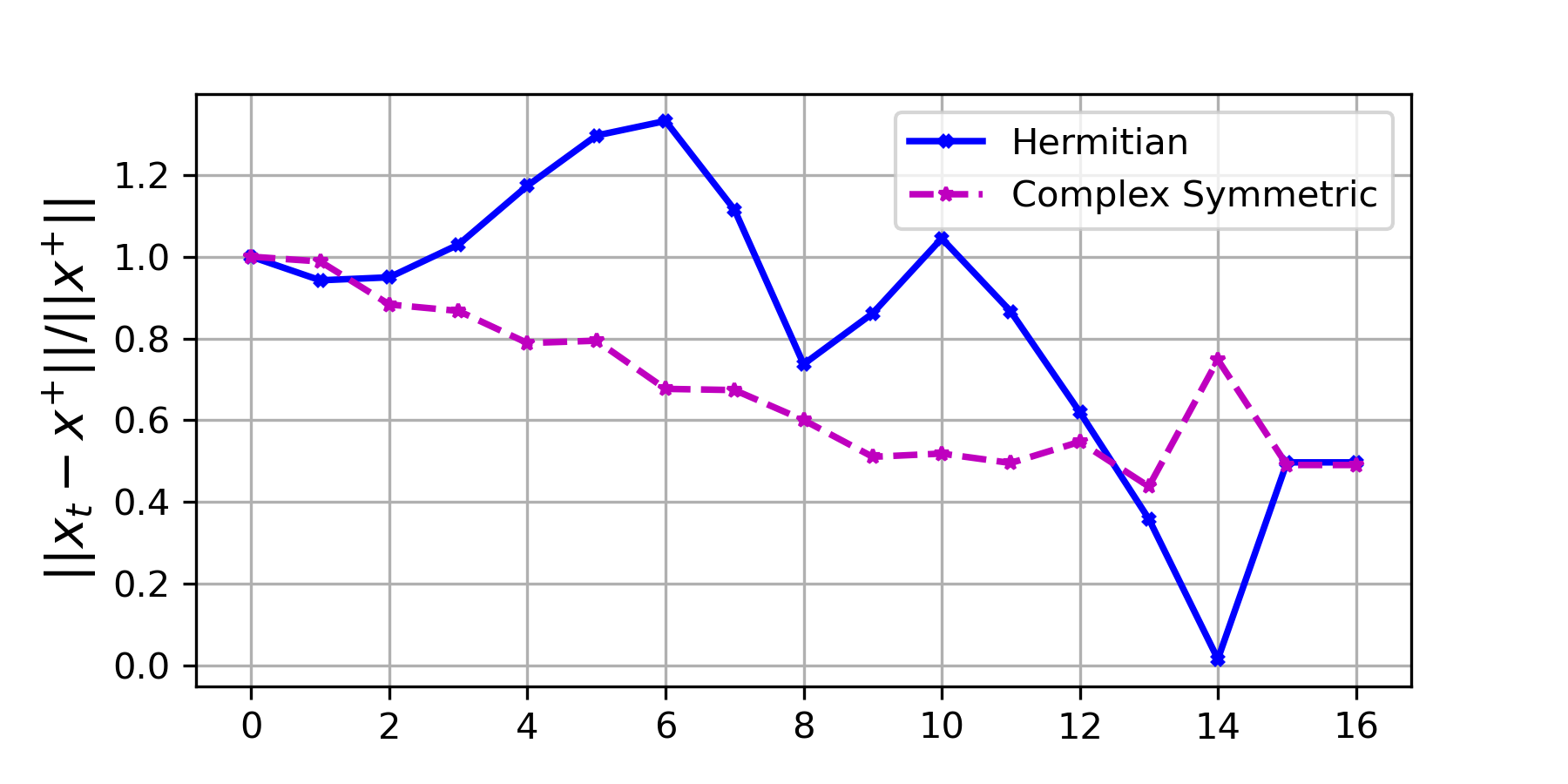
(a) Relative Error of the Plain Iterates

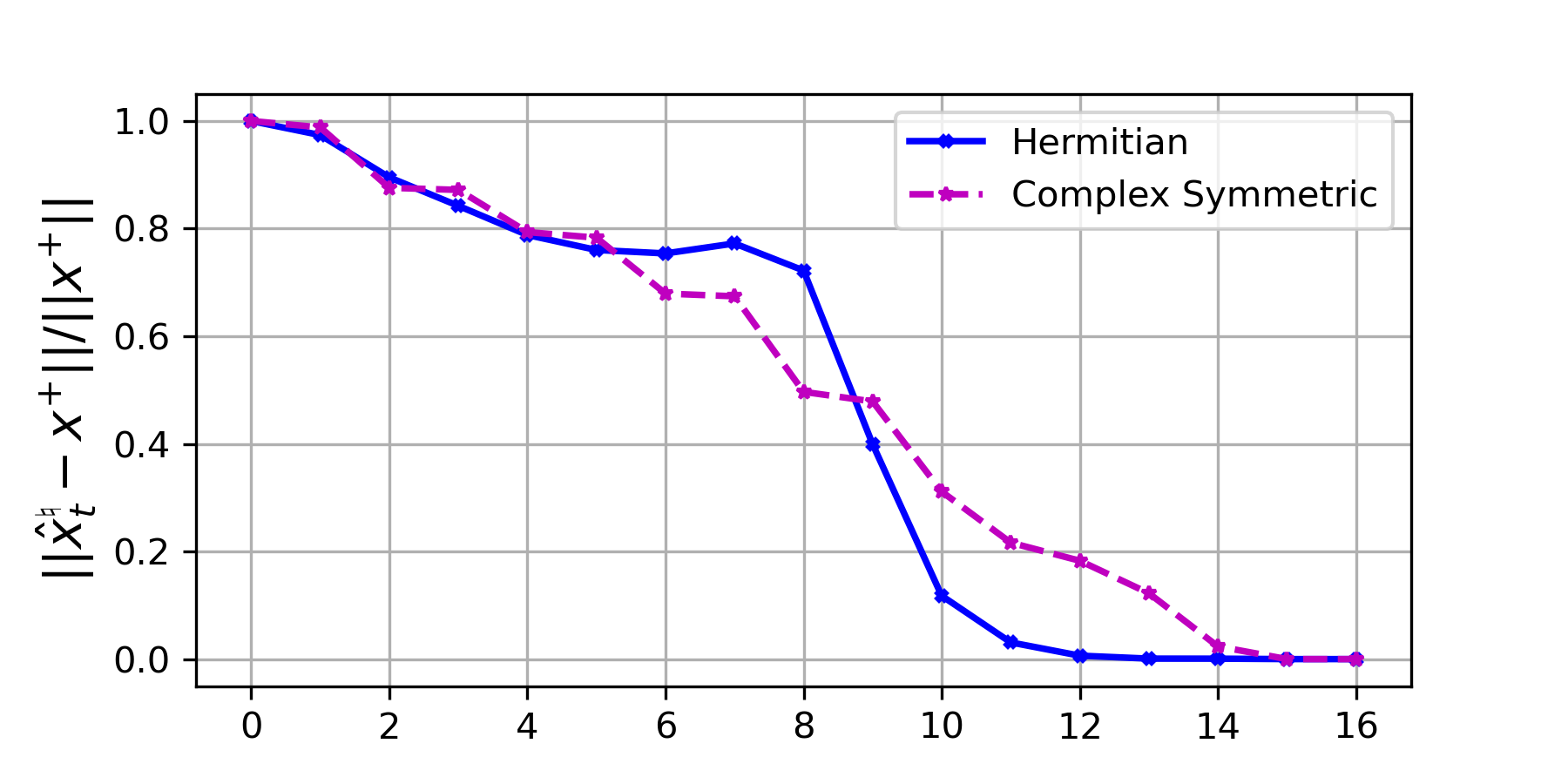
(b) Relative Error of the Lifted Iterates

Figure 1: Verifying Sections 2.1 and 2.2. Relative error of the plain (a) and lifted (b) iterates of Algorithm 1 applied to 1 with Hermitian (sold blue) and complex-symmetric (dashed magenta) matrices. The relative error is computed with respect to the pseudo-inverse solution $\mathbf{A}^{\dagger}\mathbf{b}$ in each respective case. The $x$-axis denotes the iteration counter.

Figure 2: From top to bottom: the magnitude with orientations, the X-axis components, and the Y-axis components. From left to right: the right-hand-side $\vec{f}$, the exact solution $\vec{u}_{\textnormal{exact}}$, the final MINRES iterate without lifting, and the lifted result using Section 2.1. A recorded video of this procedure can be found here.

We end this section by noting that, similar to Hermitian systems, in the case where $\mathbf{A}$ is complex-symmetric Algorithm 2 is analytically equivalent to Algorithm 3. Hence, when $m\ll d$, the sub-preconditioned algorithm Algorithm 3 can be regarded as a dimensionality reduced version of Algorithm 2 and allows for significantly less storage/computations than what is required in Algorithm 2.

4 Numerical experiments

In this section, we provide several numerical examples illustrating our theoretical findings. We first verify our theoretical results in Section 4.1 using synthetic data. We subsequently aim to explore related applications in image deblurring in Section 4.3.

4.1 Pseudo-inverse Solutions by Lifting: Sections 2.1 and 2.2

We first demonstrate Sections 2.1 and 2.2 on some simple and small synthetic problems. We consider 1 with $d=20$ and for Hermitian as well as complex-symmetric synthetic matrices. For both matrices, the rank is set to $r=15$. We also let $\mathbf{b}=\mathbf{1}$, i.e., the vector of all ones, which ensures that the right-hand side vector $\mathbf{b}$ does not lie entirely in the range of these matrices. In Figure 1, we plot the relative error of the iterates of Algorithm 1, ${\mathbf{x}}_{t}$, as well as the lifted iterates $\hat{\mathbf{x}}_{t}^{\dagger}$ using 4 and 12 to the true pseudo-inverse solution $\mathbf{x}^{+}=\mathbf{A}^{\dagger}\mathbf{b}$, namely $\|{\mathbf{x}}_{t}-\mathbf{x}^{+}\|/\|\mathbf{x}^{+}\|$ and $\|\hat{\mathbf{x}}_{t}^{\natural}-\mathbf{x}^{+}\|/\|\mathbf{x}^{+}\|$. As it can be seen from Figure 1, in sharp contrast to the plain MINRES iterates, the final lifted iterate in each setting coincides with the respective pseudo-inverse solution, corroborating the results of Sections 2.1 and 2.2.

4.2 Numerical Solution of PDEs by Lifting: Section 2.1

We consider the following Maxwell problem [44],

$$\textnormal{curl}\textnormal{ curl }\vec{u} =\vec{f}\quad\textnormal{in }\Omega$$ (46a)

$$\vec{u}\times\hat{n} =0\quad\textnormal{on }\partial\Omega$$ (46b)

where $\partial\Omega$ represents the boundary of $\Omega\in\mathbb{R}^{2}$, $\hat{n}$ is the outwards-pointing unit normal on the boundary $\partial\Omega$. We use Nédélec finite elements to discretize 46 with a regular triangular mesh with $100$ elements along each edge, resulting in $d=30,200$. The implementation of this experiment is using Firedrake [30] with a MINRES implementation from PETSc [5]. Let $\mathbf{A}$ refer to the finite element matrix associated with the discretization of curl curl operator, that is $\mathbf{A}_{ij}=\int_{\Omega}\textnormal{ curl }\vec{\phi}_{j}\cdot\textnormal{ curl }\vec{\phi}_{i}$, where $\{\vec{\phi}_{j}\}_{1}^{d}$, are basis functions spanning the Nédélec finite element space of the first kind [47]. We construct our problem in $\mathbb{R}^{2}$ with $\vec{f}=\textnormal{curl}\textnormal{ curl }\vec{u}_{\textnormal{exact}}+\vec{e}$, where $\vec{e}$ is the projection of uniformly distributed random noise $\mathcal{U}(-1,1)$ onto the null space of the operator $\mathbf{A}$. We run MINRES until $\|\mathbf{A}\mathbf{r}\|$ is sufficiently small. The termination condition is as in [41] with the tolerance $0.1$, which can be controlled via $ksp\_minres\_nutol$ option in PETSc. At termination, we apply Section 2.1 to the final iterate. The results are gathered in Figure 2, which is generated by Paraview [1]. It is clear that the MINRES final iterate, without lifting, contains a great deal of noisy features. However, we can recover a good approximation of $\vec{u}_{\textnormal{exact}}$ using Section 2.1.

4.3 Image Deblurring by Lifting: Sections 2.1 and 2

We now turn our attention to a more realistic setting in the context of image deblurring. We emphasize that our goal here is not to obtain a cutting-edge image deblurring technique that can achieve the state-of-the-art, but rather to explore the potentials of our lifting strategies in a real world application. We consider the following image blurring model

$$\mathbf{B}=\mathcal{A}(\mathbf{X})+\mathbf{E},$$

where $\mathbf{B}\in^{n\times n}$ is a noisy and blurred version of an image $\mathbf{X}\in^{n\times n}$, $\mathcal{A}:^{n\times n}\to^{n\times n}$ represents the linear Gaussian smoothing/blurring operator [56] as a 2D convolutional operator, and $\mathbf{E}$ is some noise matrix. Simple deblurring can be done by solving the least squared problem 1 where $\mathbf{x}=\textnormal{vec}(\mathbf{X})\in^{n^{2}}$, $\mathbf{b}=\textnormal{vec}(\mathbf{B})\in^{n^{2}}$, and $\mathbf{A}\in^{n^{2}\times n^{2}}$ is the real symmetric matrix representation of the Gaussian blur operator $\mathcal{A}$. Though $\mathbf{A}$ has typically full rank, it often contains several small singular values, which make $\mathbf{A}$ almost numerically singular. In lieu of employing any particular explicit regularization, we terminate the iterations early before fitting to the “noisy subspaces” corresponding to the extremely small singular values. Our aim is to investigate our lifting strategies, with or without preconditioning, for deblurring images. Specifically, we will investigate the application of 5 and 32.

When $n$ is large, it is rather impractical to explicitly store the matrix $\mathbf{A}$. To remedy this, we generate a Toeplitz matrix $\mathbf{Z}\in^{n\times n}$, from which we can implicitly define the blurring matrix $\mathbf{A}$ as $\mathbf{A}=\mathbf{Z}\otimes\mathbf{Z}$, where $\otimes$ denotes the Kronecker product. For our experiments, we consider a colored image with $n=1,024$. We solve for each channel separately and then normalize our final result to regenerate the color image. The Gaussian blurring matrix $\mathbf{A}$ is generated with bandwidth $100$ and the standard deviation of $10$. For each color channel, the elements of the corresponding noise matrix are generated i.i.d. from the standard normal distribution. Finally, we note that, in our experiments since $n\gg 1$, we apply 5 with Algorithm 3 as an equivalent alternative to applying 32 with Algorithm 2.

Deblurring with Algorithm 1 and Section 2.1

In our experiments, we first apply Algorithm 1, and evaluate the quality of the deblurred image from both unlifted solution as well as the lifted one obtained from Section 2.1. As a benchmark, we consider comparing the solutions obtained from LSQR [50], which has shown to enjoy favorable stability properties for solving large scale least-squared problems [59], as well as the standard truncated SVD. Both these methods, though not the state-of-the-art, have long been used for image deblurring problems [31, 32]. We also consider LSMR [26] as an alternative general purpose solver, as well as MINRES-QLP, which is specifically designed for solving (almost) singular systems [17]. Note that every iteration of LSQR and LSMR requires two matrix-vector multiplications whereas MINRES and MINRES-QLP involve only one such operation per iteration.

In our implementations, we set the maximum iterations for all solvers to $20,000$. Since the problem is highly ill-conditioned, instead of tracking the residual norm, we monitor the relative residual of the normal equation as $\|\mathbf{A}\mathbf{r}\|\leq 10^{-5}\|\mathbf{A}\mathbf{b}\|$. At termination of MINRES and MINRES-QLP, we apply the lifting procedure from Section 2.1 to eliminate the contributions from the noisy subspaces corresponding to extremely small singular values of $\mathbf{A}$. To evaluate the quality of the reconstructed images, we use two common metrics, namely the peak-signal-to-noise ratio (PSNR), and the structural similarity index measure (SSIM) [35, 58]. Deblurred images with higher value in either metric are deemed to be of relatively better quality.

The results are depicted in Figures 3 and 4. From Figure 3, it is clear that, LSQR not only returns a very poor solution, but it also takes the longest to terminate. Without lifting, the reconstructed image using LSMR is of higher quality compared with the ones directly obtained from Algorithm 1 and MINRES-QLP, albeit with a significantly more computation time. However, upon applying the lifting step outlined in Section 2.1, the image quality from Algorithm 1 and MINRES-QLP drastically improves, becoming highly competitive with that of LSMR, while requiring a fraction of the runtime. Although MINRES-QLP is guaranteed to recover the pseudo-inverse solution at $t=g$, it is clear that in the case of early termination and without lifting, it fails to recover a good quality solution just like MINRES; see also Section 4.3. We also apply truncated SVD [32] to give another benchmark. We can see from Figure 4, that the performance of the truncated SVD is reasonable when the singular value threshold increases. However, it is also clear that the method is highly sensitive to the choice of this threshold.

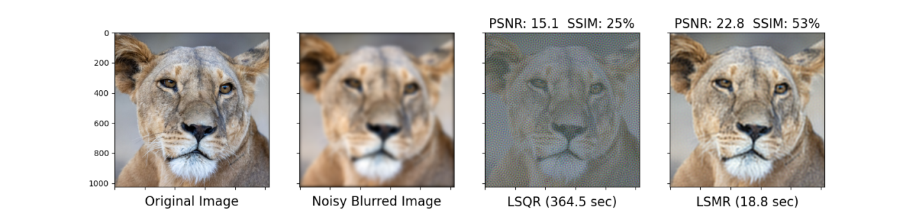
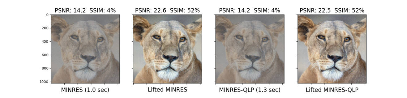
Figure 3: From the top left to the bottom right: the original image, the noisy blurred image, the image deblurred with LSQR and with LSMR; the image obtained from Algorithm 1, and the lifted image from Section 2.1, that obtained from MINRES-QLP and its corresponding lifted image from Section 2.1. The “wall-clock” time it takes in seconds for iterative algorithms to reach the inexactness.

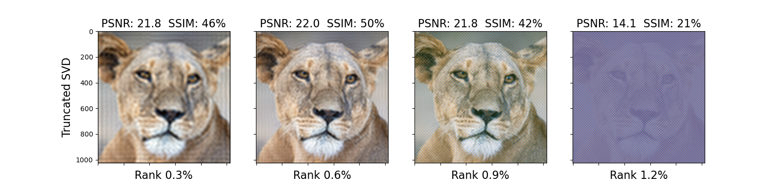
Figure 4: Image deblurring with Truncated SVD. “Rank $a$%”, “$a$%” represents the rank-ratio $r^{2}/n^{2}$, where $r$ represents the rank being used in the Truncated SVD method.

Deblurring with Algorithm 3 and 32

We now consider incorporating preconditioning withing our image deblurring problem. Recall that preconditioning has long been used in this context [22, 14, 32, 10]. To fit our settings here, we consider appropriate singular preconditioners $\mathbf{M}\succeq\mathbf{0}$, and explore the deblurring quality of the unlifted solution of Algorithm 3, as well as the lifted one by applying Section 2.1 to the preconditioned system 19.

We construct two different types of sub-preconditioners. For $i=1,2$, we let $\SS_{i}=\mathbf{C}_{i}\otimes\mathbf{C}_{i}\in^{n^{2}\times r_{i}^{2}},\;i=1,2$, where $\mathbf{C}_{i}=\mathbf{Q}_{i}\mathbf{\Sigma}_{i}\in^{n\times r_{i}},\;i=1,2$ and the factors $\mathbf{\Sigma}_{i}$, $\mathbf{Q}_{i}$ and the corresponding ranks $r_{i}$ are generated as follows:

1. To construct $\mathbf{Q}_{i}$, we first generate a $n\times n$ matrix $\hat{\mathbf{C}}$ whose elements are drawn independently from the standard normal distribution. We then choose $\mathbf{Q}_{1}\in^{n\times r_{1}}$ and $\mathbf{Q}_{2}\in^{n\times r_{2}}$ via the incomplete QR decomposition of $\mathbf{Z}\hat{\mathbf{C}}=\mathbf{Q}_{1}\mathbf{R}_{1}$ and $\hat{\mathbf{C}}=\mathbf{Q}_{2}\mathbf{R}_{2}$ with the corresponding ranks $r_{1}$ and $r_{2}$.

2. We construct the diagonal matrices $\mathbf{\Sigma}_{i}\in^{r_{i}\times r_{i}},\;i=1,2$ with positive diagonal entries such that the smallest and the largest diagonal elements are, respectively $1$ and $2$, and other elements are linearly spaced values in-between.

By construction, $\textnormal{Range}(\SS_{1})\subseteq\textnormal{Range}(\mathbf{A})$, while this is not true for $\SS_{2}$.

Considering $\SS_{2}$ as an example, we use the following Kronecker product properties to avoid explicit storage of the matrix $\mathbf{A}$:

$$\tilde{\mathbf{A}}\textnormal{vec}(\tilde{\mathbf{X}}) =\SS^{\intercal}_{2}\mathbf{A}\SS_{2}\textnormal{vec}(\tilde{\mathbf{X}})=\left(\mathbf{C}_{2}^{\intercal}\otimes\mathbf{C}_{2}^{\intercal}\right)\left(\mathbf{Z}\otimes\mathbf{Z}\right)\left(\mathbf{C}_{2}\otimes\mathbf{C}_{2}\right)\textnormal{vec}(\tilde{\mathbf{X}})$$

$$=\left(\left(\mathbf{C}_{2}^{\intercal}\mathbf{Z}\mathbf{C}_{2}\right)\otimes\left(\mathbf{C}_{2}^{\intercal}\mathbf{Z}\mathbf{C}_{2}\right)\right)\textnormal{vec}(\tilde{\mathbf{X}})=\textnormal{vec}(\mathbf{C}_{2}^{\intercal}\mathbf{Z}\mathbf{C}_{2}\tilde{\mathbf{X}}\mathbf{C}_{2}^{\intercal}\mathbf{Z}\mathbf{C}_{2})$$

$$\tilde{\mathbf{b}} =\SS^{\intercal}_{2}\textnormal{vec}(\mathbf{B})=\left(\mathbf{C}_{2}^{\intercal}\otimes\mathbf{C}_{2}^{\intercal}\right)\textnormal{vec}(\mathbf{B})=\textnormal{vec}(\mathbf{C}_{2}^{\intercal}\mathbf{B}\mathbf{C}_{2})$$

and $\mathbf{x}=\textnormal{vec}(\mathbf{X})=\SS_{2}\textnormal{vec}(\tilde{\mathbf{X}})=\left(\mathbf{C}_{2}\otimes\mathbf{C}_{2}\right)\textnormal{vec}(\tilde{\mathbf{X}})=\textnormal{vec}(\mathbf{C}_{2}\tilde{\mathbf{X}}\mathbf{C}_{2}^{\intercal})$.

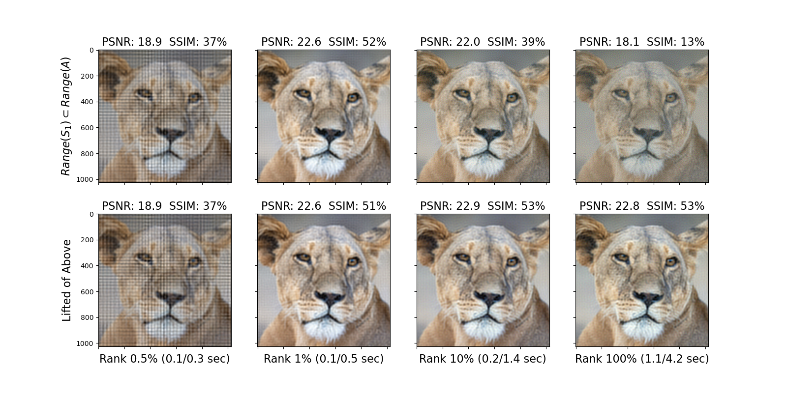
Figure 5: Image deblurring using Algorithm 3 with $\SS_{1}\in^{n^{2}\times r_{1}^{2}}$. In our naming convention, “Rank $a$% ($b$/$c$ sec)”, “$a$%” represents the rank-ratio $r_{1}^{2}/n^{2}$, “$c$” is total wall-clock time of the full deblurring process (including the incomplete QR decomposition to compute $\SS_{1}$), and “$b$” shows the time taken by Algorithm 3 only. The figures in the bottom row are the lifted versions of ones in the top row.

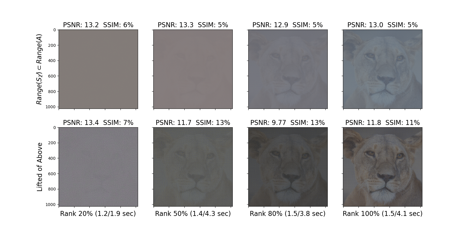
Figure 6: Image deblurring using Algorithm 3 with $\SS_{2}\in^{n^{2}\times r_{2}^{2}}$. In our naming convention, “Rank $a$% ($b$/$c$ sec)”, “$a$%” represents the rank-ratio $r_{2}^{2}/n^{2}$, “$c$” is total wall-clock time of the full deblurring process (including the incomplete QR decomposition to compute $\SS_{2}$), and “$b$” shows the time taken by Algorithm 3 only. The figures in the bottom row are the lifted versions of ones in the top row.

Figure 5 depicts the reconstruction quality using the sub-preconditioner $\SS_{1}$, where for rank-ratios larger than $1\%$, we obtain reasonable quality results. The effect of the lifting strategy from Algorithm 2 is also clearly visible, in particular for higher values of the rank-ratio. Notably, the running time of Algorithm 3 with $\SS_{1}$ makes up a small portion of the total deblurring time, including the QR decomposition to construct $\SS_{1}$. This is a direct consequence of the dimensionality reduction nature of Algorithm 3, which employs the sub-preconditioner $\SS_{1}$, as opposed to the full preconditioner $\mathbf{M}$. Also, from Figure 5 it is clear that Algorithm 3 exhibits a great degree of stability with respect to the different choices of the rank for the sub-preconditioner $\SS_{1}$, as compared with the truncated SVD in Figure 4. In Figure 6, however, we see poor quality reconstructions. This is entirely due to the fact that, by construction, $\textnormal{Range}(\SS_{2})$ does not align well with the range space of $\mathbf{A}$, and hence constitute a poor sub-preconditioner. Hence, when the underlying matrix is (nearly) singular and $\mathbf{b}$ substantially aligns with the eigen-space corresponding to small eigenvalues of $\mathbf{A}$, one should apply preconditioners that can counteract the negative effects of such alignments. This observations underlines the fact that, unlike the typical settings where the preconditioning matrix is assumed to have full-rank, the situation can be drastically different with singular preconditioners and one can face a multitude of challenges. In this respect, although singular preconditioners can be regarded as a way to reduce the dimensionality of the problem, more studies need to be done to explore various effects and properties of such preconditioners in various contexts.

Figure 3				Figure 5				Figure 6
LSQR	LSMR	MINRES	MIN-QLP	0.5%	1%	10%	100%	20%	50%	80%	100%
4,463.3	242.7	30	30	190.3	88.7	57	43.7	45	39	30.7	30

Table 1: Average number of iterations before termination for three channels using the listed solvers for the experiments of Figures 3, 6 and 5. “MIN-QLP” refers to MINRES-QLP and the “percentage values” refer to the corresponding rank-ratio defined in Figures 6 and 5.

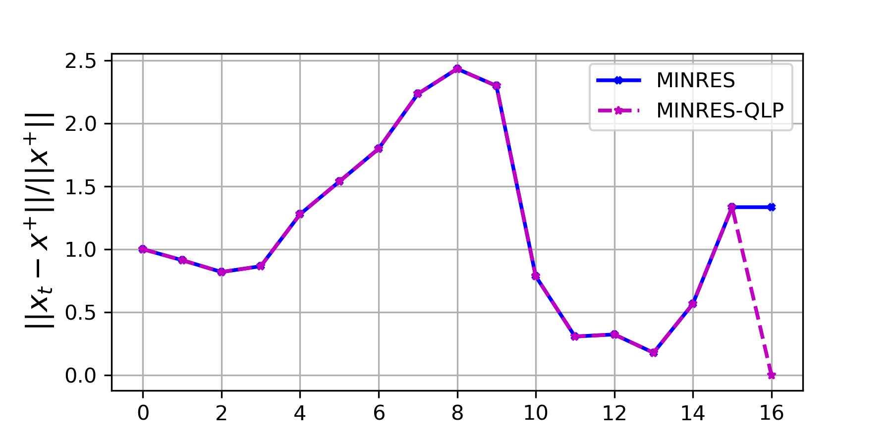
(a) Plain Iterates

(b) Lifted Iterates

Figure 7: Comparison between MINRES and MINRES-QLP, with and without lifting Section 2.1. Relative error of the plain (a) and the lifted (b) iterates of Algorithm 1 (sold blue) and MINRES-QLP (dashed magenta) applied to 1 with Symmetric matrix. The relative error is computed with respect to the pseudo-inverse solution $\mathbf{x}^{+}=\mathbf{A}^{\dagger}\mathbf{b}$. The $x$-axis denotes the iteration counter. It is clear that dynamics of plain MINRES-QLP and MINRES are almost identical expect at the very last iteration. However, the lifted iterates using Section 2.1 look almost indistinguishable.

From Figure 3 and Table 1, we see remarkable similarities between the final results of MINRES-QLP and MINRES. This warrants a further look into the dynamic of MINRES-QLP across all its iterations, as compared with MINRES. For this, we consider using both MINRES and MINRES-QLP for solving the same synthetic problem from Section 4.1 but with a symmetric matrix $\mathbf{A}$. From Figure 7, we see that the iterates from both these methods are almost identical throughout the life of the algorithms, except at the very last iteration, when $t=g=16$. This indicates that all the extra computations within MINRES-QLP at every iteration might not in fact contribute to an improved solution and it is primarily the last iteration that brings about the intended effect of obtaining the pseudo-inverse solution.

5 Conclusions

We considered the minimum residual method (MINRES) for solving linear least-squares problems involving singular matrices. It is well-known that, unless the right hand-side vector entirely lies in the range-space of the matrix, MINRES does not necessarily converge to the pseudo-inverse solution of the problem. We propose a novel lifting strategy, which can readily recover such a pseudo-inverse solution from the final iterate of MINRES. We provide similar results in the context of preconditioned MINRES using positive semi-definite and singular preconditioners. We also showed that, when such singular preconditioners are formed from sub-preconditioners, we can equivalently reformulate the original preconditioned MINRES algorithm in lower dimensions, which can be solved more efficiently. We provide several numerical examples to further shed light on our theoretical results and to explore their use-cases in some real world application.

References

• [1] James Ahrens, Berk Geveci, Charles Law, C Hansen, and C Johnson. 36-paraview: An end-user tool for large-data visualization. The visualization handbook, 717:50038–1, 2005.
• [2] GS Ammar, D Calvetti, and L Reichel. Computation of Gauss-Kronrod quadrature rules with non-positive weights. Electronic Transactions on Numerical Analysis, 9:26–38, 1999.
• [3] Peter Arbenz and Michiel E Hochstenbach. A Jacobi–Davidson method for solving complex symmetric eigenvalue problems. SIAM Journal on Scientific Computing, 25(5):1655–1673, 2004.
• [4] Rob J Arts, PN J Rasolofosaon, and BE Zinszner. Experimental determination of the complete anisotropic viscoelastic tensor in rocks. In SEG Technical Program Expanded Abstracts 1992, pages 636–639. Society of Exploration Geophysicists, 1992.
• [5] Satish Balay, Shrirang Abhyankar, Mark Adams, Jed Brown, Peter Brune, Kris Buschelman, Lisandro Dalcin, Alp Dener, Victor Eijkhout, W Gropp, et al. Petsc users manual. 2019.
• [6] Ilan Bar-On and Victor Ryaboy. A new fast algorithm for the diagonalization of complex symmetric matrices, with applications to quantum dynamics. Technical report, Society for Industrial and Applied Mathematics, Philadelphia, PA (United States), 1995.
• [7] Ilan Bar-On and Victor Ryaboy. Fast diagonalization of large and dense complex symmetric matrices, with applications to quantum reaction dynamics. SIAM Journal on Scientific Computing, 18(5):1412–1435, 1997.
• [8] Michele Benzi, Gene H Golub, and Jörg Liesen. Numerical Solution of Saddle Point Problems. Acta numerica, 14:1–137, 2005.
• [9] Dennis S Bernstein. Matrix Mathematics: Theory, Facts, and Formulas With Application to Linear Systems Theory, volume 41. Princeton University Press Princeton, 2009.
• [10] Davide Bianchi, Alessandro Buccini, and Marco Donatelli. Structure preserving preconditioning for frame-based image deblurring. In Computational Methods for Inverse Problems in Imaging, pages 33–49. Springer, 2019.
• [11] Ake Bjorck. Numerical methods for least squares problems. Siam, 1996.
• [12] Ake Bjorck. Numerical methods in matrix computations. Springer, 2015.
• [13] Angelika Bunse-Gerstner and William B Gragg. Singular value decompositions of complex symmetric matrices. Journal of Computational and Applied Mathematics, 21(1):41–54, 1988.
• [14] Ke Chen, Faisal Fairag, and Adel Al-Mahdi. Preconditioning techniques for an image deblurring problem. Numerical Linear Algebra with Applications, 23(3):570–584, 2016.
• [15] Sou-Cheng Choi. Iterative methods for singular linear equations and least-squares problems, 2006.
• [16] Sou-Cheng T Choi. Minimal residual methods for complex symmetric, skew symmetric, and skew hermitian systems, 2013.
• [17] Sou-Cheng T Choi, Christopher C Paige, and Michael A Saunders. MINRES-QLP: A Krylov subspace method for indefinite or singular symmetric systems. SIAM Journal on Scientific Computing, 33(4):1810–1836, 2011.
• [18] Sou-Cheng T Choi and Michael A Saunders. Algorithm 937: MINRES-QLP for symmetric and Hermitian linear equations and least-squares problems. ACM Transactions on Mathematical Software (TOMS), 40(2):16, 2014.
• [19] Richard Christensen. Theory of viscoelasticity: an introduction. Elsevier, 2012.
• [20] Pierre Courrieu. Fast Computation of Moore-Penrose Inverse Matrices. Neural Information Processing-Letters and Reviews, 8(2):25–29, 2005.
• [21] Yehuda Dar and Richard G Baraniuk. Double double descent: on generalization errors in transfer learning between linear regression tasks. SIAM Journal on Mathematics of Data Science, 4(4):1447–1472, 2022.
• [22] Pietro Dell’Acqua, Marco Donatelli, Claudio Estatico, and Mariarosa Mazza. Structure preserving preconditioners for image deblurring. Journal of Scientific Computing, 72(1):147–171, 2017.
• [23] Michal Derezinski, Feynman T Liang, and Michael W Mahoney. Exact expressions for double descent and implicit regularization via surrogate random design. Advances in neural information processing systems, 33:5152–5164, 2020.
• [24] Lars Elden and Valeria Simoncini. Solving ill-posed linear systems with GMRES and a singular preconditioner. SIAM Journal on Matrix Analysis and Applications, 33(4):1369–1394, 2012.
• [25] Heinz W Engl and M Zuhair Nashed. New extremal characterizations of generalized inverses of linear operators. Journal of Mathematical Analysis and Applications, 82(2):566–586, 1981.
• [26] David Chin-Lung Fong and Michael Saunders. LSMR: An iterative algorithm for sparse least-squares problems. SIAM Journal on Scientific Computing, 33(5):2950–2971, 2011.
• [27] KA Gallivan, S Thirumalai, Paul Van Dooren, and V Vermaut. High performance algorithms for Toeplitz and block Toeplitz matrices. Linear algebra and its applications, 241:343–388, 1996.
• [28] Nicholas Gould and Jennifer Scott. The state-of-the-art of preconditioners for sparse linear least-squares problems. ACM Transactions on Mathematical Software (TOMS), 43(4):1–35, 2017.
• [29] Chen Greif and James M Varah. Iterative solution of skew-symmetric linear systems. SIAM journal on matrix analysis and applications, 31(2):584–601, 2009.
• [30] David A. Ham, Paul H. J. Kelly, Lawrence Mitchell, Colin J. Cotter, Robert C. Kirby, Koki Sagiyama, Nacime Bouziani, Sophia Vorderwuelbecke, Thomas J. Gregory, Jack Betteridge, Daniel R. Shapero, Reuben W. Nixon-Hill, Connor J. Ward, Patrick E. Farrell, Pablo D. Brubeck, India Marsden, Thomas H. Gibson, Miklós Homolya, Tianjiao Sun, Andrew T. T. McRae, Fabio Luporini, Alastair Gregory, Michael Lange, Simon W. Funke, Florian Rathgeber, Gheorghe-Teodor Bercea, and Graham R. Markall. Firedrake User Manual. Imperial College London and University of Oxford and Baylor University and University of Washington, first edition edition, 5 2023.
• [31] P. C. Hansen. Rank-Deficient and Discrete Ill-Posed Problems. SIAM, 1998.
• [32] Per Christian Hansen, James G Nagy, and Dianne P O’leary. Deblurring images: matrices, spectra, and filtering. SIAM, 2006.
• [33] Magnus R Hestenes, Eduard Stiefel, et al. Methods of conjugate gradients for solving linear systems. Journal of research of the National Bureau of Standards, 49(6):409–436, 1952.
• [34] Lin-Yi Hong and Nai-Min Zhang. On the preconditioned MINRES method for solving singular linear systems. Computational and Applied Mathematics, 41(7):304, 2022.
• [35] Alain Hore and Djemel Ziou. Image quality metrics: PSNR vs. SSIM. In 2010 20th international conference on pattern recognition, pages 2366–2369. IEEE, 2010.
• [36] Victoria E Howle and Stephen A Vavasis. An iterative method for solving complex-symmetric systems arising in electrical power modeling. SIAM journal on matrix analysis and applications, 26(4):1150–1178, 2005.
• [37] Erik F Kaasschieter. Preconditioned conjugate gradients for solving singular systems. Journal of Computational and Applied mathematics, 24(1-2):265–275, 1988.
• [38] Vasilios N Katsikis, Dimitrios Pappas, and Athanassios Petralias. An improved method for the computation of the Moore–Penrose inverse matrix. Applied Mathematics and Computation, 217(23):9828–9834, 2011.
• [39] Virginia Klema and Alan Laub. The singular value decomposition: Its computation and some applications. IEEE Transactions on automatic control, 25(2):164–176, 1980.
• [40] Yang Liu and Fred Roosta. Convergence of Newton-MR under Inexact Hessian Information. SIAM Journal on Optimization, 31(1):59–90, 2021.
• [41] Yang Liu and Fred Roosta. A Newton-MR Algorithm With Complexity Guarantees for Nonconvex Smooth Unconstrained Optimization. arXiv preprint arXiv:2208.07095, 2022.
• [42] Yang Liu and Fred Roosta. MINRES: From Negative Curvature Detection to Monotonicity Properties. SIAM Journal on Optimization, 2022. Accepted.
• [43] Franklin T Luk, Sanzheng Qiao, and David Vandevoorde. Exponential Decomposition and Hankel Matrix. In INSTITUTE OF MATHEMATICS AND ITS APPLICATIONS CONFERENCE SERIES, volume 71, pages 275–286. Oxford; Clarendon; 1999, 2002.
• [44] Kent-Andre Mardal and Ragnar Winther. Preconditioning discretizations of systems of partial differential equations. Numerical Linear Algebra with Applications, 18(1):1–40, 2011.
• [45] Keiichi Morikuni and Ken Hayami. Inner-iteration krylov subspace methods for least squares problems. SIAM Journal on Matrix Analysis and Applications, 34(1):1–22, 2013.
• [46] Keiichi Morikuni and Ken Hayami. Convergence of inner-iteration gmres methods for rank-deficient least squares problems. SIAM Journal on Matrix Analysis and Applications, 36(1):225–250, 2015.
• [47] Jean-Claude Nédélec. Mixed finite elements in $\mathbb{R}^{3}$. Numerische Mathematik, 35:315–341, 1980.
• [48] ABJ ORCK and JY Yuan. Preconditioners for least squares problems by lu factorization. Electronic Transactions on Numerical Analysis, 8:26–35, 1999.
• [49] Christopher C Paige and Michael A Saunders. Solution of sparse indefinite systems of linear equations. SIAM journal on numerical analysis, 12(4):617–629, 1975.
• [50] Christopher C Paige and Michael A Saunders. LSQR: An algorithm for sparse linear equations and sparse least squares. ACM transactions on mathematical software, 8(1):43–71, 1982.
• [51] Fred Roosta, Yang Liu, Peng Xu, and Michael W Mahoney. Newton-MR: Newton’s Method Without Smoothness or Convexity. EURO Journal on Computational Optimization, 10:100035, 2022.
• [52] Miroslav Rozlozník and Valeria Simoncini. Krylov subspace methods for saddle point problems with indefinite preconditioning. SIAM journal on matrix analysis and applications, 24(2):368–391, 2002.
• [53] Yousef Saad. Iterative methods for sparse linear systems, volume 82. SIAM, 2003.
• [54] Yousef Saad. Numerical methods for large eigenvalue problems: revised edition. SIAM, 2011.
• [55] Michael A Saunders, Horst D Simon, and Elizabeth L Yip. Two conjugate-gradient-type methods for unsymmetric linear equations. SIAM Journal on Numerical Analysis, 25(4):927–940, 1988.
• [56] Linda G Shapiro and George C Stockman. Computer vision. Pearson, 2001.
• [57] Lloyd N Trefethen and David Bau III. Numerical linear algebra, volume 50. Siam, 1997.
• [58] Zhou Wang, Alan C Bovik, Hamid R Sheikh, and Eero P Simoncelli. Image quality assessment: from error visibility to structural similarity. IEEE transactions on image processing, 13(4):600–612, 2004.
• [59] Andy Wathen. Some comments on preconditioning for normal equations and least squares. SIAM Review, 64(3):640–649, 2022.