From Empirical Measurements to Augmented Data Rates: A Machine Learning Approach for MCS Adaptation in Sidelink Communication

Abstract

Due to the lack of a feedback channel in the C-V2X sidelink, finding a suitable modulation and coding scheme (MCS) is a difficult task. However, recent use cases for vehicle-to-everything (V2X) communication with higher demands on data rate necessitate choosing the MCS adaptively. In this paper, we propose a machine learning approach to predict suitable MCS levels. Additionally, we propose the use of quantile prediction and evaluate it in combination with different algorithms for the task of predicting the MCS level with the highest achievable data rate. Thereby, we show significant improvements over conventional methods of choosing the MCS level. Using a machine learning approach, however, requires larger real-world data sets than are currently publicly available for research. For this reason, this paper presents a data set that was acquired in extensive drive tests, and that we make publicly available.

Keywords: SDR, V2X, Sidelink, MCS Prediction, Machine learning, Mode-4.

I Introduction

Recently, vehicle-to-everything (V2X) communication has gained a lot of attention due to its potential to increase road safety, traffic efficiency, but also to support autonomous driving technologies, for example, by extending on-board sensors with information from the infrastructure. Sidelink communication, as introduced by 3GPP in the LTE and 5G standards [1], has the advantage that it can operate both, in cellular coverage, where certain configuration is provided by the base station (BS) (called Mode 3 in LTE V2X), and out-of-coverage, where the user equipments (UEs) autonomously configure themselves (called Mode 4 in LTE V2X). Although in many of today’s most common sidelink use cases only very few information messages are transmitted, more recent use cases, which involve video transmissions [2], require significantly higher goodput. Here, it is paramount to configure the sidelink according to the propagation conditions, and thus methods for choosing good transmission parameters are required [3]. One solution for this problem is to use machine learning (ML) algorithms, which, however, requires training data. While training data for cellular communication can be found easily [4, 5, 6], there is a lack of available training data for sidelink communications. Most of the existing literature focuses on very specific scenarios, and their measurements are not publicly available for use in ML-related research [7, 8, 9].

Due to the lack of sidelink measurement data, we conducted an extensive drive test in the city of Berlin. Our drive test route contains different geographical areas, including a park, a highway, and a tunnel in order to get a very diverse data set that is representative of real-world use. By using our own full-stack sidelink implementation [10], we could gather data with very high time resolution. Our data set has been made publicly available in order to facilitate further research on ML methods for sidelink communication.

One important aspect of the Mode 4 specifications is that there is no feedback channel that can adapt transmission parameters based on the channel link quality [11]. In many research studies, the authors have tried to add adaptation capability to C-V2X without changing the protocol. For example, vehicle location and speed were used as side-channel information for optimizing the communications [3]. In another study, the authors propose to adapt transmission power and control message intervals in highly dense environments with severe collisions and interference, to improve the packet reception ratio (PRR) [12]. In a subsequent study, the authors demonstrate a multi-agent deep reinforcement learning-based algorithm in sensing-based Semi-Persistent Scheduling (SPS) to select resources more intelligently and to reduce packet collisions over unmodified V2X Mode 4 [13].

The main contributions of our paper are mainly in two areas. Firstly, we have generated a real-world data set by extensive drive tests through a set of different geographical locations and also made this data set public for further research. Secondly, we have ventured into the issue of fixed transmission parameters in 3GPP V2X ( Mode 4 ) Release 14 by employing a machine learning based modulation and coding scheme (MCS) adaption, which permits more flexible data transmission in varying channel conditions. Eventually, in the case of LTE sidelink, we achieve significantly higher goodputs than the best possible non-adaptive method.

We organized the rest of this paper as follows. First, Section II describes the measurement setup and the data set we acquired for our evaluation. Next, Section III presents the algorithms we used for maximizing goodput. Then, in Section IV, we compare the prediction performance of different algorithms. Finally, in Section V, we highlight the main findings.

II Drive test data set

In the following, we describe the hardware setup which we used to perform the measurements, followed by a presentation of the data processing steps and some statistical properties of the data set.

For sidelink communication, we used a software defined radio (SDR) sidelink unit that was previously developed in [10]. The general setup is shown schematically in Figure 1. The sidelink case is equipped with a sidelink antenna and a global positioning system (GPS) antenna, both of which we attached to the roof of the car. Two cars were equipped with one sidelink unit each. Transmission was done with a center frequency of $5.9\text{\,}\mathrm{G}\mathrm{H}\mathrm{z}$ and a transmit power of $17.3\text{\,}\mathrm{d}\mathrm{B}\mathrm{m}$. Both sidelink units were synchronized using GPS timestamps.

Usually, the sidelink standard prevents sending data every millisecond but requires larger intervals to also give other users transmission opportunities. However, in order to collect enough data, we modified the sidelink Mode 4 software from [10] in order to quickly sweep over all available MCS levels (0 to 19). Moreover, we use one sidelink unit as a dedicated transmitter and the second one as dedicated receiver. We disabled any sensing-based scheduling algorithms in order to use all the 48 resource block (RB) for transmission while sweeping over MCS levels. More specifically, a single large packet whose size is chosen to fully utilize the available throughput is transmitted for $1\text{\,}\mathrm{m}\mathrm{s}$ with a specific MCS level, after which we switch to the next MCS level. The second sidelink unit acts as a dedicated receiver and writes every successfully decoded data packet into a packet capture (PCAP) based trace for offline analysis. Additionally, physical layer measurements like signal-to-noise ratio (SNR), reference signal received power (RSRP), and received signal strength indicator (RSSI) are also saved to the PCAP file.

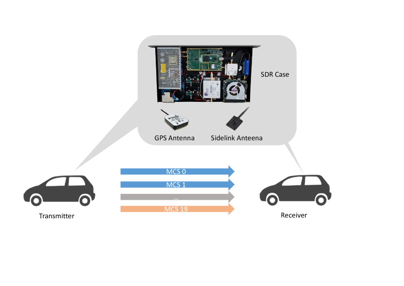
Figure 1: Schematic description of measurement setup [10].

For processing, we parse the information about the successfully decoded packets from the PCAP file. Due to the fact that one packet was sent per millisecond, we can reconstruct which packets could not be successfully decoded. The physical layer measurements for the missing packets are then reconstructed using linear interpolation from the surrounding packets. Finally, we aggregate each MCS sweep and save the highest MCS level that could be successfully decoded, while taking the mean of the physical layer measurements. This highest usable MCS level can then be used as a target for the prediction algorithms. Context information from GPS is then merged according to the timestamp.

In order to gather data in a diverse set of conditions, we devised the route shown in Figure 2, which contains an avenue, a park, a highway, a residential area, and a tunnel in Berlin. Data was collected from two cars driven in close proximity for a total of six rounds during the course of one day. In total, we have collected 608542 samples.

Figure 2: Test Drive Route (©2023 GeoBasis-DE/BKG (©2009), Google).

Information was collected from a total of two sources, namely physical layer measurements from the UE (named Base), and positional information from GPS (named Positions). Table I shows the list of all available features.

TABLE I: Overview of available features.

Group	Source	Features
Base	UE	Signal-to-noise ratio (SNR), reference signal received power (RSRP), received signal strength indicator (RSSI), Noise power, Rx power
Positions	GPS	Latitude, Longitude, Velocity

Subsequently, we summarize a statistical analysis of the collected data set. In Figure 3, we show the continuous probability density of the RSRP, where the different areas refer to the ones shown in Figure 2. The packet error rate (PER) for different MCS levels split by area is shown in Figure 4. The reason that the residential area, tunnel, and park have generally lower PERs than avenue and highway can be attributed to lower distances, which are due to the lower average driving speeds in these geographical areas. In order to further evaluate the influence of distance on PER, we show the PER for different distances and MCS levels in Figure 5. The (inverse) correlation between distance and PER can be clearly seen.

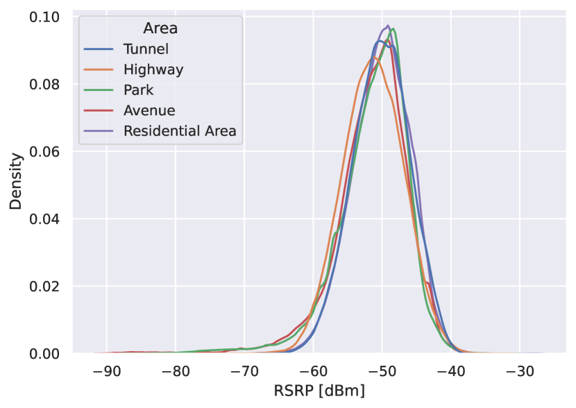
Figure 3: KDE of RSRP of different geographical areas.

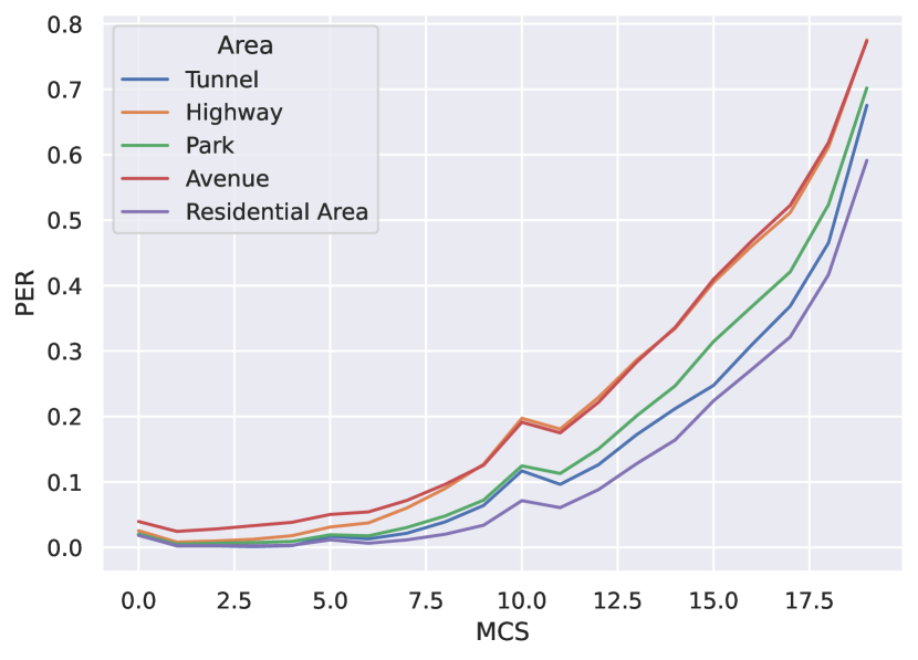
Figure 4: PER of different MCS levels of different geographical area.

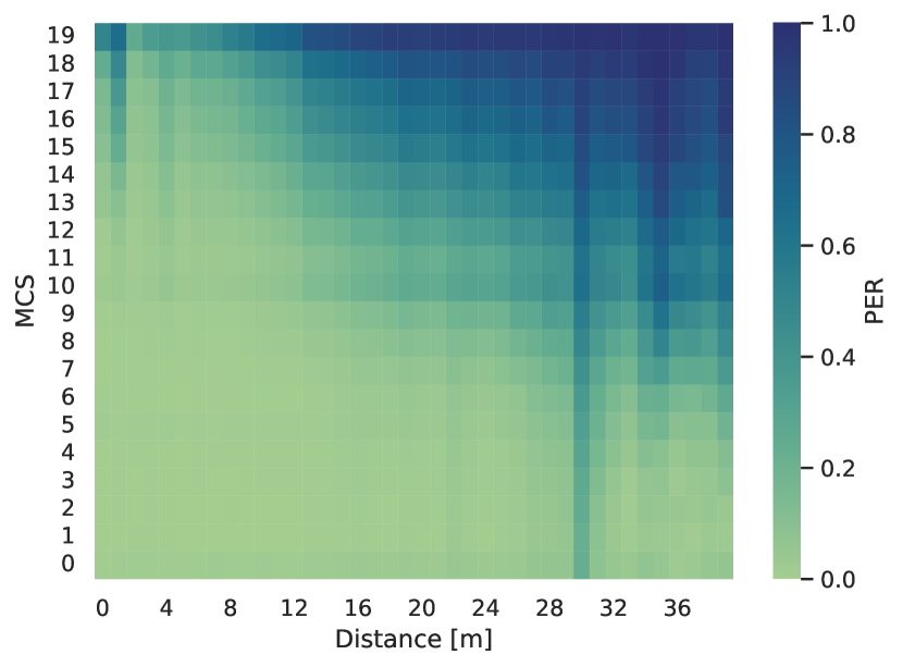
Figure 5: PER for different MCS levels and distances.

III Machine Learning Approach

In the following, we present the machine learning algorithms that we used to predict the optimal MCS level, followed by information on hyperparameter optimization and on the general evaluation methodology.

We evaluated a total of four algorithms, random forest (RF) [14, 15], gradient boosting (GB) [16], neural network (NN), and Linear regression (LR). The architecture of NN contains a feed-forward neural network with the features as input, a number of hidden layers, and the predicted MCS level as a single output, using a fully connected topology. The hidden layers employ an activation function, while L1/L2 regularization is used to prevent over-fitting. As an optimizer, we use Adam. The number of hidden layers, number of neurons, and activation functions are treated as hyperparameters that are to be optimized. In addition to these algorithms, as a baseline, we consider the highest goodput that could be achieved by using a fixed MCS for all packets. In the context of this study, we consider goodput to be the amount of data that can be successfully decoded at the receiver.

Due to the fact that we try to predict the MCS level, our main problem is the inherently asymmetric objective function, i.e., over-predicting the MCS level will lead to not decodable packets and thus 0 goodput, while under-predicting the MCS level will lead to only a slightly reduced goodput. To deal with this asymmetric nature, we use quantile prediction, which we implemented by using the pinball loss function for NN and GB and by using quantile regression forests [15] instead of regular RFs. The pinball loss function is defined as

$$\mathcal{L}_{\tau}(y,\hat{y})=\left\{\begin{array}[]{rcl}\tau(y-\hat{y})&\mbox{if}&y\geq\hat{y}\\ (1-\tau)(\hat{y}-y)&\mbox{if}&y<\hat{y},\\ \end{array}\right.$$ (1)

where $\tau$ is the desired quantile and $y$ and $\hat{y}$ are the measured and predicted MCS levels, respectively [17]. The desired quantile $\tau$ will be treated as a hyper-parameter that is to be optimized. Minimizing pinball loss with LR is usually done by means of solving a linear programming problem [18]. However, this is not possible for large data sets due to prohibitive computational complexity. For this reason, the results in this paper for LR generally refer to the results derived via the ordinary least squares algorithm, which minimizes the mean square error (MSE). When the results explicitly refer to quantile regression, we derived these results by using stochastic gradient descent (SGD).

In pursuit of hyperparameter optimization, we apply a randomized search over a suitably defined probability distribution for each parameter. We chose a randomized search where we employed the leave one group out method as our cross-validation technique. Leaving one group out uses one round as test data, and the remaining ones as training data, until each unique round has served as a test set once. This comprehensive hyperparameter optimization method bolsters the robustness and generalization of the model to perform reliably across different real-world environments. By employing this approach, we get a set of results and their corresponding hyperparameters. From them, we considered the hyperparameters that gave the best result for RF, GB, and NN with 100 iterations. Due to the cost of computation, we ran hyperparameter optimization once per algorithm.

What remains is to determine the optimal set of features. In order to do so, we attempt to order the features by importance. A simple approach to do so is to calculate the correlation between the features and the target. The result is shown in Figure 6, where it can be seen that MCS level has the strongest correlation to the features that are related to signal strength (i.e., SNR, RSRP, RSSI and receive power). However, we note that this approach has serious limitations as it only captures linear dependencies not casual dependencies [19].

In order to better capture the impact that the individual features have on the quality of prediction, we additionally employ the more powerful permutation feature importance method [14]. Permutation feature importance measures the decrease in model performance when the values for a specific feature are randomly shuffled. Using this method, we determined that the features sorted by importance are SNR, Rx power, RSSI, distance, RSRP, noise power, speed (of user 2 and 1), latitude (of user 2 and 1), longitude (of user 2 and 1), and Rx gain.

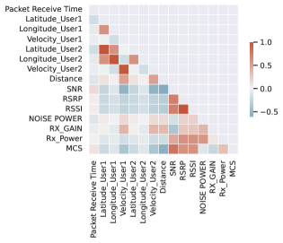
Figure 6: Pearson correlation coefficients between different features and MCS.

IV Prediction results

In order to evaluate the performance of the algorithms defined above, we used one round of the drive data as a test set and the remaining rounds as a training set. We repeated this process for each round and took the average of all rounds. As a performance metric, we calculated the throughput by multiplying the transport block size for the (rounded) predicted MCS level and 48 RBs according to the 3GPP standard [20, Table 8.6.1-1, 7.1.7.2.1-1] with 1000 transport blocks per second. We then considered this throughput to be goodput, unless the predicted MCS level was larger than the highest usable MCS level, in which case we set the achievable goodput to 0 for this sample.

First, we looked at the influence of the number of features that are used for prediction on the achievable goodput. In order to do so, we sorted the features based on importance according to the method introduced above, and trained the models using only the $N$ most important features. As shown in Figure 7, it can be clearly seen that the performance increases with an increasing number of features for all algorithms except linear regression. However, the performance increase from using more than four features is very small, so in a practical implementation, where computational complexity is a restricting factor, only the four most important features should be used.

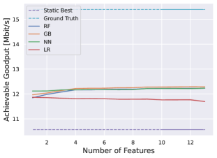
Figure 7: Achievable goodput for different number of features.

Next, we look at the performance of the different algorithms when only a reduced number of training samples is available. As shown in Figure 8, neural networks need a much larger number of training samples to achieve satisfactory performance, while for the other algorithms increasing the number of training samples only gives a small improvement in performance. This behavior is consistent with the literature [21].

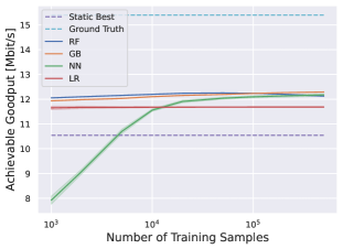
Figure 8: Predicted goodput for a varying number of training samples. Shaded regions show the standard deviation of the mean.

Since using all available training samples and features provides the best results, we use this configuration in a final performance assessment. As shown in Table II, the algorithm with the best performance is GB, while NN and RF show similar performance. For comparison, the ground truth gives a goodput of $15.397\text{\,}\mathrm{M}\mathrm{b}\mathrm{i}\mathrm{t}\mathrm{/}\mathrm{s}$, while using the best static MCS level gives a goodput of $10.541\text{\,}\mathrm{M}\mathrm{b}\mathrm{i}\mathrm{t}\mathrm{/}\mathrm{s}$. In order to assess the effectiveness of our quantile regression approach, we compare our results to conventional regression algorithms. This comparison shows that by using quantile regression the goodput is increased by about $0.5\text{\,}\mathrm{M}\mathrm{b}\mathrm{i}\mathrm{t}\mathrm{/}\mathrm{s}$ over using MSE loss as loss function and by about $0.8\text{\,}\mathrm{M}\mathrm{b}\mathrm{i}\mathrm{t}\mathrm{/}\mathrm{s}$ over using mean absolute error (MAE) loss, regardless of the algorithm, thus demonstrating the effectiveness of using quantile regression.

TABLE II: Prediction results based on different loss functions.

	Achievable Goodput [$\mathrm{M}\mathrm{b}\mathrm{i}\mathrm{t}\mathrm{/}\mathrm{s}$]
Algorithm	Quant. Reg.	MSE	MAE
Gradient Boosting	$12.295$	$11.880$	$11.520$
Neural Network	$12.263$	$11.818$	$11.490$
Random Forest	$12.232$	$11.794$	$11.456$
Linear Regression	$12.033$	$11.736$	$11.549$

V Conclusions

In this paper, we describe the measurement setup and the resulting data set of an extensive sidelink measurement campaign in a realistic urban setting. Based on the collected data, we train machine learning algorithms to optimize the MCS to maximize the goodput. We demonstrated that significantly higher goodput can be achieved by the machine-learning aided dynamic selection than those achieved by fixed configuration policies, and we additionally show the benefits including vehicle location, velocity, and distance to other vehicles as features to predict MCS. Furthermore, our approach does not require any feedback information or any modifications to the current protocol.

The proposed approach dynamically changes the MCS and our results show more than $16\text{\,}\%$ gain in goodput compared to the theoretically best possible result achievable using fixed transmission configuration policies in our real-world data set. In practice, we expect the achieved gains to be even higher, since it is highly difficult to select in advance the MCS that will provide the best results. In real-world scenarios, the environment changes rapidly, due to changing distances, the presence of physical obstruction, and interference, and these factors contribute to frequent channel condition fluctuation.

The collected data set has been made fully available in order to be used not only in MCS prediction (for example, by evaluating the performance of a reinforcement learning agent for the prediction task), but also for other ML-aided optimization research.

References

- [1] M. H. C. Garcia, A. Molina-Galan, M. Boban, J. Gozalvez, B. Coll-Perales, T. Şahin, and A. Kousaridas, “A tutorial on 5g nr v2x communications,” IEEE Communications Surveys & Tutorials, vol. 23, no. 3, pp. 1972–2026, 2021.
- [2] B. Zhang, E. S. Wilschut, D. Willemsen, T. Alkim, and M. H. Martens, “The effect of see-through truck on driver monitoring patterns and responses to critical events in truck platooning,” in International Conference on Applied Human Factors and Ergonomics. Springer, 2017, pp. 842–852.
- [3] Y.-J. Ku, B. Flowers, S. Thornton, S. Baidya, and S. Dey, “Adaptive c-v2x sidelink communications for vehicular applications beyond safety messages,” in 2022 IEEE 95th Vehicular Technology Conference:(VTC2022-Spring). IEEE, 2022, pp. 1–6.
- [4] B. Sliwa and C. Wietfeld, “Empirical Analysis of Client-based Network Quality Prediction in Vehicular Multi-MNO Networks,” 2019 IEEE 90th Vehicular Technology Conference (VTC2019-Fall), pp. 1–7, Sep. 2019.
- [5] D. Schäufele, M. Kasparick, J. Schwardmann, J. Morgenroth, and S. Stańczak, “Terminal-side data rate prediction for high-mobility users,” in 2021 IEEE 93rd Vehicular Technology Conference (VTC2021-Spring). IEEE, 2021, pp. 1–5.
- [6] A. Palaios, P. Geuer, J. Fink, D. F. Külzer, F. Göttsch, M. Kasparick, D. Schäufele, R. Hernangómez, S. Partani, R. Sattiraju et al., “Network under control: Multi-vehicle e2e measurements for ai-based qos prediction,” in 2021 IEEE 32nd Annual International Symposium on Personal, Indoor and Mobile Radio Communications (PIMRC). IEEE, 2021, pp. 1432–1438.
- [7] I. Rodriguez, E. P. Almeida, M. Lauridsen, D. A. Wassie, L. C. Gimenez, H. C. Nguyen, T. B. Sørensen, and P. Mogensen, “Measurement-based evaluation of the impact of large vehicle shadowing on v2x communications,” in European Wireless 2016; 22th European Wireless Conference. VDE, 2016, pp. 1–8.
- [8] F. De Ponte Müller, I. Rashdan, M. Schmidhammer, and S. Sand, “Its-g5 and c-v2x link level performance measurements,” 2021.
- [9] S. Hüsges, M. Meuleners, N. Bateni, and C. Degen, “Simulation and measurement for sidelink communication between cars and bicycles,” in 2022 16th European Conference on Antennas and Propagation (EuCAP). IEEE, 2022, pp. 1–5.
- [10] R. Lindstedt, M. Kasparick, J. Pilz, and S. Jaeckel, “An open software-defined-radio platform for lte-v2x and beyond,” pp. 1–5, 2020.
- [11] R. Molina-Masegosa, J. Gozalvez, and M. Sepulcre, “Configuration of the c-v2x mode 4 sidelink pc5 interface for vehicular communication,” in 2018 14th International conference on mobile ad-hoc and sensor networks (MSN). IEEE, 2018, pp. 43–48.
- [12] B. Kang, J. Yang, J. Paek, and S. Bahk, “Atomic: Adaptive transmission power and message interval control for c-v2x mode 4,” IEEE Access, vol. 9, pp. 12 309–12 321, 2021.
- [13] B. Gu, W. Chen, M. Alazab, X. Tan, and M. Guizani, “Multiagent reinforcement learning-based semi-persistent scheduling scheme in c-v2x mode 4,” IEEE Transactions on Vehicular Technology, vol. 71, no. 11, pp. 12 044–12 056, 2022.
- [14] L. Breiman, “Random forests,” Machine learning, vol. 45, no. 1, pp. 5–32, 2001.
- [15] N. Meinshausen and G. Ridgeway, “Quantile regression forests.” Journal of machine learning research, vol. 7, no. 6, 2006.
- [16] T. Chen and C. Guestrin, “Xgboost: A scalable tree boosting system,” in Proceedings of the 22nd acm sigkdd international conference on knowledge discovery and data mining, 2016, pp. 785–794.
- [17] Y. Wang, D. Gan, M. Sun, N. Zhang, Z. Lu, and C. Kang, “Probabilistic individual load forecasting using pinball loss guided lstm,” Applied Energy, vol. 235, pp. 10–20, 2019.
- [18] R. Koenker, Quantile regression. Cambridge university press, 2005, vol. 38.
- [19] J. L. Rodgers and W. A. Nicewander, “Thirteen ways to look at the correlation coefficient,” The American Statistician, vol. 42, no. 1, pp. 59–66, 1988. [Online]. Available: http://www.jstor.org/stable/2685263
- [20] T. ETSI, “136 213 v13. 0.0,” ETSI standard, 2016.
- [21] H. Xu, K. A. Kinfu, W. LeVine, S. Panda, J. Dey, M. Ainsworth, Y.-C. Peng, M. Kusmanov, F. Engert, C. M. White et al., “When are deep networks really better than decision forests at small sample sizes, and how?” arXiv preprint arXiv:2108.13637, 2021.