Diffusion Models as Stochastic Quantization in Lattice Field Theory

Abstract

In this work, we establish a direct connection between generative diffusion models (DMs) and stochastic quantization (SQ). The DM is realized by approximating the reversal of a stochastic process dictated by the Langevin equation, generating samples from a prior distribution to effectively mimic the target distribution. Using numerical simulations, we demonstrate that the DM can serve as a global sampler for generating quantum lattice field configurations in two-dimensional $\phi^{4}$ theory. We demonstrate that DMs can notably reduce autocorrelation times in the Markov chain, especially in the critical region where standard Markov Chain Monte-Carlo (MCMC) algorithms experience critical slowing down. The findings can potentially inspire further advancements in lattice field theory simulations, in particular in cases where it is expensive to generate large ensembles.

1 Introduction

To obtain physical observables in lattice field theory, it is essential to approximate the path integral as a sum over field configurations. Monte Carlo methods rely on random sampling from the probability distribution, determined by the action of the system Knechtli:2017sna . These methods can have high computational costs, particularly in the vicinity of a critical point in parameter space Wolff:1989wq . Generative models, as a class of machine learning (ML) algorithms, can be trained to generate new data that follow the same distribution as a given data set, representing the underlying target distribution tomczak:2022deep . An important potential application of generative models in lattice QCD is therefore to improve the efficiency of Monte Carlo simulations Boyda:2022nmh .

Depending on the way the likelihood is estimated, roughly two main categories of generative models are being developed. In implicit maximum likelihood estimation (MLE), Generative Adversarial Networks (GANs) can learn to generate new configurations via a min-max game using training on a dataset prepared using, e.g., a standard lattice simulation. A well-trained GAN can subsequently generate new samples, which should follow the same statistical distribution as the original dataset, but with reduced computational cost. Additionally, GANs can be used to improve the interpretability of lattice QCD simulations by generating visualizations of the system’s behavior Zhou:2018ill ; Pawlowski:2018qxs . In explicit MLE, flow-based models have recently been proposed to improve the efficiency of lattice simulations Albergo:2019eim ; Kanwar:2020xzo ; Nicoli:2020njz ; Albergo:2021bna ; Albergo:2021vyo ; DelDebbio:2021qwf ; Hackett:2021idh ; Albergo:2022qfi ; Bacchio:2022vje ; Caselle:2022acb ; Chen:2022ytr ; Gerdes:2022eve ; Albandea:2023wgd ; Singha:2023cql . Flow-based models are able to directly approach the underlying distribution of the quantum field without preparing training data. Although the method may encounter “mode-collapse” and scalability problems Abbott:2022zsh ; Nicoli:2023qsl , it allows for the generation of independent new configurations that can be used in MC simulations, again reducing the computational cost. The current progress in applying generative models also includes designing novel neural network architectures for specific field theories, e.g., autoregressive networks Wang:2020hji ; Luo:2023opo and gauge-equivariant neural networks Favoni:2020reg ; Kanwar:2020xzo ; Aronsson:2023rli ; Abbott:2022zhs ; Gerdes:2022eve ; Luo:2023opo . These approaches suggest that generative models have the potential to advance the capabilities of lattice QCD simulations. A comprehensive review can be found in Refs. Zhou:2023pti ; He:2023zin .

Recently, the ML community has developed a new class of deep generative models known as Diffusion Models yang:2022diffusion . Impressive success has been obtained in generating high-quality images via stochastic denoising processes, as showcased in prominent applications Croitoru:2023dm such as DALL-E 2 2022arXiv220406125R and Stable Diffusion Rombach_2022_CVPR . As a prevalent class of generative models encoded in a stochastic process, DMs are grounded in Markov chains, and their implementation involves the utilization of variational inference methods. For an adoption in high-energy physics experiments, see, e.g., Refs. Mikuni:2022xry ; Mikuni:2023dvk .

In numerical lattice field theory, there is an approach alternative to Monte Carlo methods to generate field configurations which relies on solving a stochastic differential equation, i.e., a Langevin equation. Its origin is stochastic quantization (SQ) as proposed by Parisi and Wu Parisi:1980ys . The basic idea of SQ is to view the quantum system as the thermal equilibrium limit of a hypothetical stochastic process with respect to a fictitious time. For gauge fields, it does not require gauge fixing Parisi:1980ys . Comprehensive reviews include Refs. Damgaard:1987rr ; Namiki:1993fd . For theories with a sign or complex weight problem, such as Quantum Chromodynamics at nonzero baryon density or theories in real (rather than Euclidean) time, the Langevin process can be extended to complex Langevin dynamics Parisi:1983mgm , which evades the sign problem in certain cases Berges:2006xc ; Aarts:2008rr ; Aarts:2008wh ; Seiler:2012wz ; Sexty:2013ica , see also the reviews Aarts:2015tyj ; Attanasio:2020spv ; Berger:2019odf ; Nagata:2021ugx . Although the method has been put on firmer theoretical grounds Aarts:2009uq ; Aarts:2011ax ; Nagata:2016vkn ; Aarts:2017vrv ; Scherzer:2018hid , convergence and boundary condition issues continue to hinder obtaining a fully satisfying approach. Recent work to address this includes Refs. WesthHansen:2022iqd ; Alvestad:2021hsi ; Alvestad:2022abf ; Lampl:2023xpb .

In this work, we first point out the correspondence between generative Diffusion Models (DMs) from the ML community and SQ in quantum field theory. Then, we explore using DMs to generate lattice field configurations. Specifically, we demonstrate for a two-dimensional $\phi^{4}$ lattice field theory that, combined with a hybrid Monte Carlo (HMC) algorithm, DMs can serve as an efficient global sampler along a Markov chain, leading to shorter autocorrelation times. We provide self-consistency checks and numerical evidence that this approach is able to capture the SQ perspective-induced stochastic dynamics of quantum field theories.

The paper is organized as follows. In the subsequent section, we provide a brief overview of the concept of SQ. In Sec. 3, we present details of DMs. It is argued that the denoising process of DMs can explicitly serve as a SQ procedure. In Sec. 4, we explore the application of DMs to a two-dimensional scalar $\phi^{4}$ field theory. Additionally, we demonstrate that DMs can accurately estimate the physical action in an unsupervised manner using the probabilistic flow approach. In Sec. 5, we summarize the correspondence between DMs and SQ, and outline how this novel method can motivate further research, in particular for theories where it is expensive to sample from the prior distribution using standard approaches. App. A contains information on the U-Net architecture employed.

2 Stochastic Quantization

In Euclidean quantum field theory, as an alternative quantization scheme, one may invoke stochastic quantization (SQ) Parisi:1980ys . We only consider real actions here, for which SQ is well understood and convergence is guaranteed Damgaard:1987rr . Starting from a generic Euclidean path integral with Euclidean action $S_{E}$,

$$Z=\int D\phi\,e^{-S_{E}},$$ (1)

SQ introduces a fictitious time, $\tau$, for the field, $\phi$, whose evolution is described by Langevin dynamics,

$$\frac{\partial\phi(x,\tau)}{\partial\tau}=-\frac{\delta S_{E}[\phi]}{\delta\phi(x,\tau)}+\eta(x,\tau),$$ (2)

where the noise term routinely satisfies,

$$\langle\eta(x,\tau)\rangle=0,\qquad\langle\eta(x,\tau)\eta(x^{\prime},\tau^{\prime})\rangle=2\alpha\delta(x-x^{\prime})\delta(\tau-\tau^{\prime}),$$ (3)

with $\alpha$ being the diffusion constant. Denoting the distribution as

$$p(\phi)=\frac{e^{-S_{E}(\phi)}}{Z},$$ (4)

the drift term in the Langevin equation can be written as

$$K(\phi)\equiv-\frac{\delta S_{E}}{\delta\phi(x)}=\frac{\delta\log p(\phi)}{\delta\phi(x)}.$$ (5)

In the long-time limit ($\tau\rightarrow\infty$) the system reaches an equilibrium state of the dynamics Namiki:1993fd if the drift term has a damping effect, which is best analysed using the Fokker-Planck equation (see below). In addition, introducing the stochasticity is only one strategy for the quantization. The fictitious time itself can serve as a clue to develop microcanonical quantization, which describes a deterministic evolution with an ordinary differential equation Callaway:1982eb . We will revisit this idea and its connection with diffusion models in Sec. 3.3.

2.1 Fokker-Planck Equation and Observables

The Fokker-Planck equation risken1996fokker describes the time evolution of the probability distribution of field configurations, subject to a stochastic process, such as the Langevin equation. Also known as the Kolmogorov forward equation, in the context of SQ it describes the time evolution of the probability density function $P[\phi,\tau]$ for field configurations $\phi$ at time $\tau$ Damgaard:1987rr ; Namiki:1992wf , as follows,

$$\frac{\partial P[\phi,\tau]}{\partial\tau}=\int d^{n}x\left\{\frac{\delta}{\delta\phi}\left(\alpha\frac{\delta}{\delta\phi}+\frac{\delta S_{E}}{\delta\phi}\right)\right\}P[\phi,\tau].$$ (6)

Here $n$ is the dimension of the Euclidean spacetime on which the field theory is formulated. Given this probability distribution function, the expectation value of an observable $\mathcal{O}[\phi]$ is then given by Damgaard:1987rr

$$\langle\mathcal{O}[\phi]\rangle_{\tau}=\int D\phi\,\mathcal{O}[\phi]P[\phi,\tau],$$ (7)

where the left-hand side is understood as an average over many stochastic processes and on the right-hand side the integral is taken over all field configurations $\phi$.

In the long-time limit, the probability distribution $P[\phi,\tau]$ should approach an equilibrium distribution, which is the stationary solution of the Fokker-Planck equation (6),

$$P_{\text{eq}}[\phi]\propto e^{-\frac{1}{\alpha}S_{E}[\phi]}.$$ (8)

If $\alpha$ is set (formally) as $\hbar$ and the equilibrium distribution is normalised, expectation values of observables are indeed observables in a quantum theory, with

$$\langle\mathcal{O}[\phi]\rangle_{\tau\to\infty}=\frac{\int D\phi\,\mathcal{O}(\phi)e^{-\frac{1}{\hbar}S_{E}(\phi)}}{\int D\phi\,e^{-\frac{1}{\hbar}S_{E}(\phi)}}=\langle\mathcal{O}[\phi]\rangle_{\text{quantum}},$$ (9)

demonstrating that a stochastic process according to Eq. (2) can be used to quantize a system. Note that convergence to the stationary solution (8) follows from properties of the Fokker-Planck Hamiltonian associated to the Fokker-Planck equation (6) Damgaard:1987rr .

2.2 Simulations

In most cases, the Fokker-Planck equation cannot be solved analytically. Instead, one solves the stochastic process numerically by discretizing the Langevin equation Eq. (2). Using Itô calculus, the simplest discretized Langevin equation, using time step $\Delta\tau$, is

$$\phi(x,\tau_{n+1})=\phi(x,\tau_{n})+K[\phi(x,\tau_{n})]\Delta\tau+\sqrt{\Delta\tau}\eta(x,\tau_{n}),$$ (10)

with $\langle\eta(x,\tau_{n})\eta(x^{\prime},\tau_{n^{\prime}})\rangle=2\alpha\delta(x-x^{\prime})\delta_{nn^{\prime}}$.

A typical calculation includes, firstly, an initial condition to prepare field configurations $\{\phi(x,\tau=0)\}$; secondly, the thermalization procedure, i.e, evolve the system to reach equilibrium by iterating through a sufficient number of time steps, $T$, with an appropriate time step, $\Delta\tau$; thirdly, after thermalization, record the values of the physical observable $\mathcal{O}[\phi]$ for each configuration in an ensemble. This is repeated for numerous configurations to improve the statistical accuracy of the ensemble average. Fig. 1 demonstrates one such typical Langevin process for a one-dimensional case.

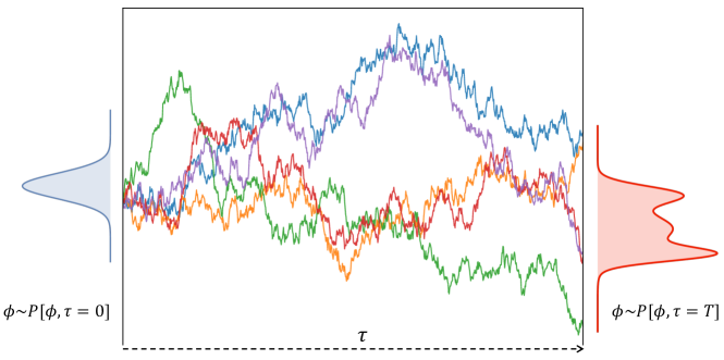
Figure 1: Sketch of a Langevin simulation. Each line represents a different trajectory, evolving from an initial state to a sufficiently long time, $T$. The initial configurations are sampled from a prior but naive distribution, $\phi\sim P[\phi,\tau=0]$. After the simulation, the final configurations follow the equilibrated distribution, $\phi\sim P[\phi,\tau=T]\sim P_{\rm target}[\phi]$.

This procedure provides an estimate of the quantum expectation value for the observable $\mathcal{O}[\phi]$. Since the simple discretization above results in finite-stepsize errors linear in $\Delta\tau$, one has to repeat the analysis to extrapolate to vanishing stepsize. The Langevin simulation provides an alternative to Monte Carlo approaches and has been used in simulations of lattice QCD Batrouni:1985jn . A feature is that no accept/reject step is used.

3 Diffusion Models

Turning now to deep learning, diffusion models (DMs) denote a class of deep generative algorithms that simulate a stochastic process to generate samples following a desired target distribution sohl-dickstein:2015deep . The fundamental concepts underlying DMs involve modeling the data distribution through a continuous-time diffusion process or a discrete-time Markov chain, wherein noise is incrementally added to or removed from the data. This generative framework has gained prominence in recent works, such as score-based models (SBMs) NEURIPS2019_3001ef25 ; song2021scorebased and denoising diffusion probabilistic models (DDPMs) ho:2020denoising ; for a comprehensive review, see Ref. yang:2022diffusion . In this section, we will first introduce the denoising perspective of DMs and then point out the connections of DMs to stochastic quantization.

3.1 Denoising Model

In the context of diffusion models, the denoising model can be perceived as a mapping that reconstructs the original data from its noisy variant, which is attained through the application of a diffusion process. Similar to the Langevin dynamics introduced above, the first process (also called forward process) gradually introduces noise to the data, effectively “smoothing” the underlying (but typically unknown) probability distribution of data. Then the denoising model aims to learn its inverse process, i.e., denoising the data by eliminating the added noise. Upon training, the denoising model can be employed to generate samples following the data distribution by executing the reverse diffusion process only. This sampling process commences with random noise and iteratively applies the trained denoising model to “clean” it until convergence, resulting in a sample representative of the target data distribution.

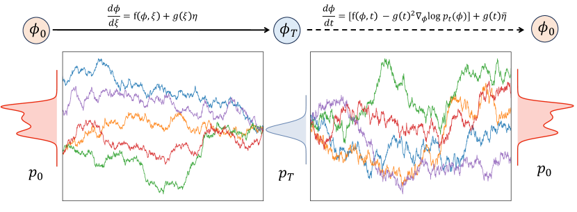
Figure 2: A sketch of the forward diffusion process (left panel) and the reverse denoising process (right panel). The two stochastic processes are described by two stochastic differential equations. The target distribution is typically unknown but learnt from the training data.

In the limit of continuous time, the forward process follows a stochastic differential equation (SDE),

$$\frac{d\phi}{d\xi}=f(\phi,\xi)+g(\xi)\eta(\xi),$$ (11)

where $\xi\in[0,T]$ is the Langevin time, $\eta$ is the noise term, satisfying $\langle\eta(\xi^{\prime})\eta(\xi^{\prime})\rangle=2\delta(\xi-\xi^{\prime})$, and $f(\phi,\xi)$ is the drift term. Note that the noise and drift term have the same dimension as the field $\phi$. Finally, the square of $g(\xi)$ is the scalar diffusion coefficient, which is time-dependent. The forward diffusion process can be modeled as the solution of such a generic SDE, provided the drift and diffusion coefficient are chosen appropriately.

As Fig. 2 demonstrates, the aim is to obtain a sample from the data distribution $p_{0}$ by starting from a sample of the prior distribution $p_{T}$ and reversing the above diffusion process. This is achieved by solving a reverse SDE, representing a diffusion process evolving backward in time, which reads anderson:1982reversetime

$$\frac{d\phi}{dt}=\left[f(\phi,t)-g^{2}(t)\nabla_{\phi}\log p_{t}(\phi)\right]+g(t)\bar{\eta}(t),$$ (12)

where the reverse time $t\equiv T-\xi$ and $\bar{\eta}$ is a noise term in the reverse time direction. Importantly, the drift term now contains two terms, including the gradient of the logarithm of $p_{t}(\phi)$, the probabilistic distribution at time $t$ in the forward diffusion process. This reverse SDE can be computed once we have specified the drift term and diffusion coefficient of the forward SDE, and determined the gradient of $\log p_{t}(\phi)$ for each $t\in[0,T]$.

The key to implementing a denoising model lies in accurately estimating the probability distribution, $p_{t}(\phi)$, under a well-designed forward diffusion process of Eq. (11). In score-based models NEURIPS2019_3001ef25 ; song2021scorebased , $\nabla_{\phi}\log p_{t}(\phi)$ is named as the score of each sample. Routinely, one can introduce a perturbation kernel for each forward diffusion step as $p_{\xi}(\phi_{\xi}|\phi_{0})\equiv\mathcal{N}(\phi_{\xi};\phi_{0},\sigma_{\xi}^{2}\mathbf{I})$, where $\phi_{0}\sim p_{0}$. Thus, the score can be computed from

$$p_{\xi}(\phi)=\int p_{\xi}(\phi_{\xi}|\phi_{0})p_{0}(\phi_{0})d\phi.$$ (13)

A neural network $\mathbf{s}_{\theta}(\phi,t)$ can be trained to approach the score conveniently, which is named as score matching Aapo:2005scb ; Vincent:2011scb . The parameters of the neural network are optimized with the objective,

$$\mathcal{L}_{\theta}=\sum_{i=1}^{N}\sigma_{i}^{2}\mathbb{E}_{p_{0}(\phi_{0})}\mathbb{E}_{p_{i}(\phi_{i}\mid\phi_{0})}\left[\left\|\mathbf{s}_{\theta}(\phi_{i},\xi)-\nabla_{\phi_{i}}\log p_{i}(\phi_{i}|\phi_{0})\right\|_{2}^{2}\right],$$ (14)

where the interval $T$ has been divided into $N$ segments with index $i$ (further details are given below). The optimal score-based model $\mathbf{s}_{\hat{\theta}}(\phi,t)$ with $\hat{\theta}=\arg\operatorname*{min}_{\theta}\mathcal{L}_{\theta}$ should match the score at every time-step. Sampling turns to solving the reverse SDE shown in Eq. (12), however, with the score being replaced with $\mathbf{s}_{\hat{\theta}}(\phi,t)$,

$$\frac{d\phi}{dt}=\left[f(\phi,t)-g^{2}(t)\mathbf{s}_{\hat{\theta}}(\phi,t)\right]+g(t)\bar{\eta}(t).$$ (15)

For a concrete and concise example, by eliminating the forward drift term $f(\phi,\xi)$ and simplifying the diffusion coefficient, see, e.g., Ref. song2021scorebased , as $g(\xi)\equiv\sigma^{\xi}$, one gets a variation expanding forward process whose transition kernel remains Gaussian,

$$p_{\xi}(\phi_{\xi}|\phi_{0})=\mathcal{N}\bigg{(}\phi_{\xi};\phi_{0},\frac{1}{2\log\sigma}(\sigma^{2\xi}-1)\mathbf{I}\bigg{)}.$$ (16)

We note that both Eqs. (11) and (12) are Langevin equations. In the context of the reverse SDE, given the gradients $\nabla_{\phi}\log p(\phi,t)$, it is convenient to generate samples from a prior distribution in a Markov chain of updates, as introduced in Sec. 2.2.

3.2 Diffusion Model as Stochastic Quantization

The reverse SDEs of diffusion models are mathematically related to the Langevin dynamics. To explore the connection of diffusion models to stochastic quantization in more detail, we choose the variance expanding picture of the diffusion models. Its denoising process transfers $\phi_{T}$ back to $\phi_{0}$ with the same marginal densities as the forward process, but evolving according to

$$\frac{d\phi}{dt}=-g(t)^{2}\nabla_{\phi}\log{p_{t}(\phi)}+g(t)\bar{\eta}(t),$$ (17)

where time $t$ flows backward from $T$ to 0. With the redefinition of time, $\tau\equiv T-t$ ($d\tau\equiv-dt$), and denoting $g_{\tau}=g(T-\tau)$, $q_{\tau}(\phi)=p_{T-\tau}(\phi)$ of the forward process, the SDE now reads

$$\frac{d\phi}{d\tau}=g_{\tau}^{2}\nabla_{\phi}\log{q_{\tau}(\phi)}+g_{\tau}\bar{\eta}(\tau)\\$$ (18)

and in discretised form

$$\phi(\tau_{n+1})=\phi(\tau_{n})+g_{\tau_{n}}^{2}\nabla_{\phi}\log{q_{\tau_{n}}[\phi(\tau_{n})]}\Delta\tau+g_{\tau_{n}}\sqrt{\Delta\tau}\bar{\eta}(\tau_{n}),$$ (19)

where the noise term $\langle\bar{\eta}(\tau_{n})\rangle=0,\langle\bar{\eta}(\tau_{n})\bar{\eta}(\tau_{n^{\prime}})\rangle=2\bar{\alpha}\delta_{nn^{\prime}}$, with $\bar{\alpha}=1$. Because the mean value of the noise term remains zero, the sign in front of the noise term is unrelated to the stochastic process. We note that $g^{2}(\tau)$ is referred to as a kernel, rescaling both the drift term and the variance of the noise term Damgaard:1987rr . Its effect can be absorbed by rescaling time with $g^{2}(\tau)$, or equivalently absorb it in the time step, $g_{\tau}^{2}\Delta\tau$.

The derivation of the corresponding Fokker-Planck is straightforward and one finds

$$\frac{\partial p_{\tau}(\phi)}{\partial\tau}=\int d^{n}x\left\{g^{2}_{\tau}\frac{\delta}{\delta\phi}\left(\bar{\alpha}\frac{\delta}{\delta\phi}+\nabla_{\phi}S_{\text{DM}}\right)\right\}p_{\tau}(\phi),$$ (20)

where

$$\nabla_{\phi}S_{\text{DM}}\equiv-\nabla_{\phi}\log{q_{\tau}(\phi)}$$ (21)

is the score trained on the forward diffusion process, and $p_{\tau}(\phi)$ is the probability density of $\phi_{\tau}$ in the reverse diffusion process. One can immediately derive the following equilibrium condition, locally in time,

$$p_{\text{eq}}(\phi)\propto e^{-S_{\text{DM}}/\bar{\alpha}},$$ (22)

where we recall that $\bar{\alpha}=1$ and that $S_{\text{DM}}$ is an effective action that will be learned in diffusion models. When the noise scales are on par with the quantum scale, that is, $O(\bar{\alpha})\sim O(\hbar)$, Eq. (22) encompasses the quantum fluctuations exhibited in Equation (8). In the $\tau\rightarrow T$ limit, $p_{\tau=T}(\phi)\rightarrow P[\phi,T]$, where $P[\phi,T]$ is nothing but the time evolution of the PDF in SQ. This implies that the “equilibrium state” of SQ can be achieved by denoising from a naive distribution. Concurrently, sampling from a diffusion model is equivalent to optimizing a stochastic trajectory to approach the “equilibrium state” in Eq. (8) given a naive distribution from the SQ perspective.

However, reverting the noise configuration back to the physics configuration is a highly intricate process. In principle, one could solve the reverse SDE of Eq. (18) to depict this denoising process, while computing the “time-dependent” drift term remains intractable. A particular type of deep neural network, known as the U-Net, is used here. The architecture of this network is discussed in more detail in the App. A. The U-Net is tailored to parameterize the score function, $\hat{\mathbf{s}}_{\theta}(\phi,\tau)$, for estimating this “time-dependent” drift term, $-\nabla_{\phi}\log{q_{\tau}(\phi)}$. It is designed to accept two inputs: time and a time-dependent configuration within a trajectory, while its output is the same size as the input.

3.3 Continuous Flow

The probability flow ODE formulation Maoutsa:2020ode ; song2021scorebased provides a way to compute the negative log-likelihood which is nothing but the effective action for the field system. Assuming a differentiable one-to-one mapping $\mathbf{h}$ that transforms a data sample $\phi\sim p_{0}$ to a prior distribution $\mathbf{h}(\phi)\sim p_{T}$, the likelihood of $p_{0}(\phi)$ can be computed using the change-of-variable formula as

$$p_{0}(\phi)=p_{T}(\mathbf{h}(\phi))|\operatorname{det}(J_{\mathbf{h}}(\phi))|,$$ (23)

where $J_{\mathbf{h}}(\phi)$ denotes the Jacobian of the mapping $\mathbf{h}$, and it is assumed that the prior distribution $p_{T}$ is easy to be evaluated. ODE trajectories also define a one-to-one mapping from $\phi_{0}$ to $\phi_{T}$. In our case,

$$\frac{d\phi}{dt}=\left[f(\phi,t)-g(t)^{2}\nabla_{\phi}\log p_{t}(\phi)\right].$$ (24)

It aims to find the trajectory of the state variable $\phi$ that has the same marginal probability density $p_{t}(\phi)$ as the stochastic process described by the SDE, i.e., Eq. (11). An instantaneous change-of-variable formula can be derived to connect the probability of $p_{0}(\phi)$ and $p_{T}(\phi)$, as,

$$p_{0}(\phi_{0})=\exp\left[\int_{0}^{T}dt\,\mathbf{\nabla}\cdot f(\phi_{t},t)\right]p_{T}(\phi_{T}),$$ (25)

where the divergence is the trace of the Jacobian. The practical computation of the trace can be found in App. B by using the Skilling-Hutchinson estimator grathwohl2018scalable .

From the perspective of probability current conservation, the stochastic process we derived in the previous section intrinsically connects with flow-based models, which have recently been widely explored in current lattice calculations Albergo:2021vyo ; Zhou:2023pti . In a flow-based model, one constructs a flow mapping to build a bijective transformation between the physical distribution, $p(\phi)$, and a prior distribution, e.g., $\mathbf{z}\sim\mathcal{N}(\mathbf{0},\mathbf{I})$. Although it is common to build the flow mapping in discrete steps, the transformation $f$ which follows,

$$\log p(\phi)=\log p(\mathbf{z})-\log\left|\text{det}\frac{\partial f}{\partial\mathbf{z}}\right|,$$ (26)

can also be designed in continuous steps. It refers to the continuous normalizing flow Gerdes:2022eve , in which the parameterized mapping, $f_{\hat{\theta}}$, is the solution to a neural ODE for time $t\in[0,T]$,

$$\frac{d\phi(t)}{dt}=f_{\theta}[\phi(t),t],$$ (27)

with boundary conditions: $\phi(0)\equiv\mathbf{z}$, $\phi(T)\equiv\phi$. A neural network with parameters $\{\theta\}$, $g_{\theta}(\phi,t)$, can be introduced to represent the dynamical kernel, whose well-tuned version corresponds to $f_{\theta}$. The probabilistic flow follows,

$$\frac{d\log p[\phi(t)]}{dt}=-\left(\nabla_{\phi}\cdot f_{\theta}\right)[\phi(t),t],$$ (28)

with boundary $p(\phi(0))\equiv p(\mathbf{z})$. Comparing the mapping and ODEs in Eqs. 23 and 24 with Eqs. 26 and 27, one can immediately find that the flow mapping, $f_{\theta}[\phi(t),t]$, is equivalent to the drift term, $f(\phi,t)$, in a reverse ODE for diffusion models.

3.4 Effective Action in a Toy Model

From Eqs. (18) and (20), one can find a “time-dependent” stochastic process. In the variance-expanding DM model, the forward process of Eq. (11) features a “predetermined” time-dependent diffusion noise denoted as $\sigma^{T-\tau}$, which can ensure field configurations will eventually be reduced to a noise configuration. The effective action and the corresponding denoising process can be understood from a field deformation perspective: the field is continuously deformed following a stochastic process from the noise distribution to the physical distribution.

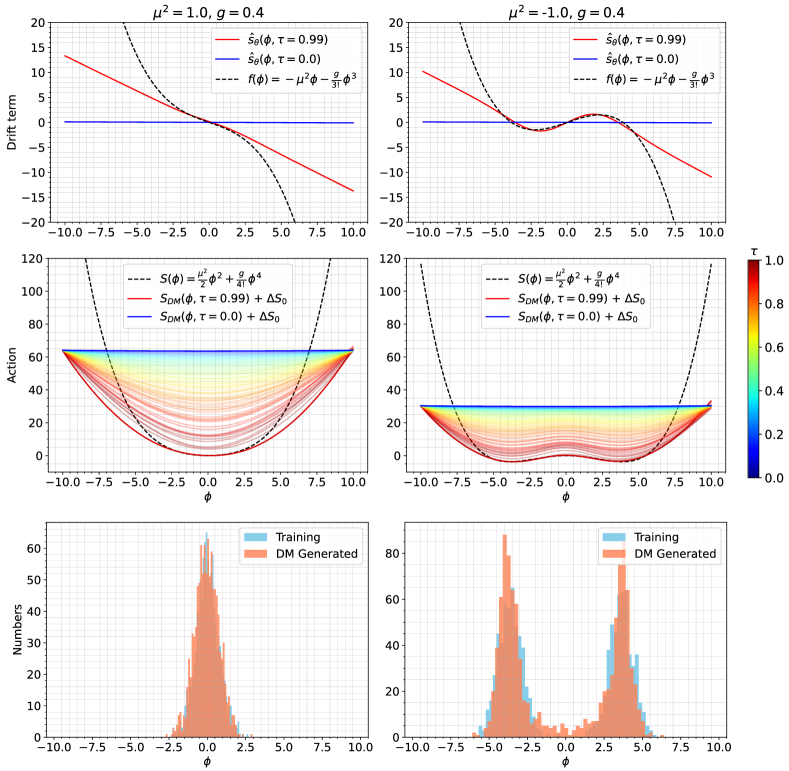
Figure 3: Drift terms (upper row) and effective actions (middle row) learned by the diffusion model as a function of $\phi$ in both single-well (left column) and double-well (right column) actions, for various values of the time $\tau$ during the stochastic process. The action is shifted by a constant $\Delta S_{0}$. The dashed lines indicate the exact values. 1024 samples generated using the exact and the diffusion model are shown in the bottom row.

To demonstrate this in action, we introduce an over-simplified 0+0-dimensional field theory, i.e., a toy model which only has one degree of freedom,

$$S(\phi)=\frac{\mu^{2}}{2}\phi^{2}+\frac{g}{4!}\phi^{4},\qquad f(\phi)=-\frac{\partial S(\phi)}{\partial\phi}=-\mu^{2}\phi-\frac{g}{3!}\phi^{3},$$ (29)

where the physical action and drift term are determined by parameters, $\mu^{2}$ and $g$. We prepared 5120 configurations as training data-sets in two set-ups: $\mu_{1}^{2}=1.0,g_{1}=0.4$ (single-well action), and $\mu_{2}^{2}=-1.0,g_{2}=0.4$ (double-well action). A one-to-one neural network with time-embedding is implemented to represent the score function $\mathbf{s}_{\theta}(\phi,\tau)$.

After 500 epochs of training, the learned score function $\hat{\mathbf{s}}_{\theta}(\phi,\tau)$ is seen to approximate the drift term $f_{\tau}(\phi)$ in the upper row of Fig. 3. Here the solid blue line represents the score function at the starting time ($\tau=0$), the rainbow-colored lines indicate different $\tau>0$ with a color-bar at rightest, while the solid red line indicates the score function at the end time ($\tau=0.99$) in a backward process of the well-trained DM. The learned effective action $S_{\text{DM}}(\phi,\tau)=\int^{\phi}\hat{\mathbf{s}}_{\theta}(\tilde{\phi},\tau)d\tilde{\phi}$ is shown in the middle row of Fig. 3; it approximates the physical action as $\tau$ increases. We have shifted $S_{\text{DM}}$ with a constant $\Delta S_{0}$, which is the difference between $\min[S(\phi)]$ and $\min[S_{\text{DM}}(\phi,\tau)]$. Generally, the learned drift terms and effective actions are accurate approximations in both the single and double-well cases, around $\phi\sim 0$. Samples generated with the trained DM are compared with samples from the underlying theory in the bottom row of Fig. 3.

The evolution trajectory of DM resembles an exact renormalizing group (RG) flow and its inversion. One intuitive understanding is that the gradually increasing noise scale (in the forward process of the DM) in coordinate space implicitly corresponds to a gradually decreasing momentum scale $\Lambda$ in an RG. With $g_{\tau\rightarrow T}=\sigma^{T-\tau}\rightarrow 1$, $\Lambda\rightarrow\infty$, the full quantum theory is recovered. Although some works have discussed the running noise scales from a colored noise perspective in a Langevin process Bern:1986xc ; Pawlowski:2017rhn , the well-trained DM provides an exact RG flow in the fictitious time space,

$$\frac{\partial S_{\text{DM}}(\phi,\tau)}{\partial\tau}=\frac{\partial}{\partial\tau}\int^{\phi}\hat{\mathbf{s}}_{\theta}(\tilde{\phi},\tau)d\tilde{\phi}.$$ (30)

Because the probability density is positive-definite, the equation gives a fixed point when $\partial p_{\tau}(\phi)/\partial\tau=0$. The RG flow is the evolution trajectory of the system from the trivial distribution at $\tau=0$ to the equilibrium state at $\tau=T$, which has been shown in the middle panel of Fig. 3.

4 Diffusion Models for Lattice $\phi^{4}$ Scalar Fields

Lattice scalar field theories have been studied extensively, with applications spanning a wide range of topics. Scalar fields are frequently employed to showcase the efficacy of numerical algorithms, including with machine learning. Here we will implement a diffusion model to generate configurations for a two-dimensional scalar field theory with quartic interaction, both in the broken and the symmetric phase.

We consider a real scalar field in $d$ Euclidean dimensions with the action,

$$S_{E}=\int\text{d}^{d}x\left(\frac{1}{2}\sum_{\mu=1}^{d}\left(\partial_{\mu}\phi_{0}\right)^{2}+\frac{1}{2}m_{0}^{2}\phi_{0}^{2}+\frac{\lambda_{0}}{4!}\phi_{0}^{4}\right),$$ (31)

where the subscript specifies bare quantities, including mass $m_{0}$, coupling $\lambda_{0}$, and field $\phi_{0}(x)$. Discretising the derivative on a lattice with lattice spacing $a$ in all directions, $\partial_{\mu}\phi_{0}(x)=[\phi_{0}(x+a\hat{\mu})-\phi(x)]/a$, with $\hat{\mu}$ the unit vector along the $\mu-$direction, and redefining the field and parameters to yield dimensionless combinations, gives the lattice action (see e.g. Ref. Smit:2002ug )

$$S_{E}=\sum_{x}\left[-2\kappa\sum_{\mu=1}^{d}\phi(x)\phi(x+\hat{\mu})+(1-2\lambda)\phi^{2}(x)+\lambda\phi^{4}(x)\right],$$ (32)

where $\kappa$ is the hopping parameter, related to the bare mass parameter via

$$(am_{0})^{2}=\frac{1-2\lambda}{\kappa}-2d,$$ (33)

and $\lambda=a^{4-d}\kappa^{2}\lambda_{0}/6$ denotes the dimensionless coupling constant describing field interactions. Both parameters are positive. The field has been rescaled according to $a^{d/2-1}\phi_{0}=(2\kappa)^{1/2}\phi$.

In the case of $d\geq 2$, for each coupling $\lambda$ the hopping parameter exhibits a critical value $\kappa_{c}(\lambda)$, at which a second-order phase transition occurs. This quantum phase transition corresponds to a spontaneous $\mathbb{Z}_{2}$ symmetry broken above the critical point in continuum limit Akiyama:2021zhf . When the mass term becomes negative, the broken phase emerges classically. At the classical level, the critical value for the hopping parameter is given by

$$\kappa_{\text{c}}^{\rm cl}(\lambda)=\frac{1-2\lambda}{2d},$$ (34)

which is determined by the vanishing of the mass term, but quantum fluctuations will change the value Smit:2002ug . As $\kappa$ decreases across the critical value, the system transitions from the broken phase to the symmetric phase.

4.1 Configuration Generation and Model Setups

To implement the diffusion model, we first prepare field configurations of the scalar $\phi^{4}$-theory in $d=2$ dimensions on a $32\times 32$ lattice, at fixed $\lambda=0.022$, as defined above. To evaluate the performance of the model, we generated 5120 samples for training and 1024 samples for testing in the broken and symmetric phases at $\kappa=0.5$ and $\kappa=0.21$ respectively. The reason to choose these specific paramter values is that at $\lambda=0.022$ the phase transition occurs at approximately $\kappa_{c}\simeq 0.239$, as derived from Eq. (34).

Hybrid Monte Carlo set-up. In order to prepare the dataset, we employ the Monte Carlo Markov Chain (MCMC) approach. The classical Metropolis-Hastings algorithm for local updating often suffers from long autocorrelation times, so we instead opt for the hybrid Monte Carlo (HMC) method. By incorporating classical Hamiltonian equations of motion neal2011mcmc , the HMC method improves the performance of the MCMC and allows larger steps to be taken while maintaining acceptable acceptance rates. In our setup with the selected set of action parameters on a 2-dimensional $32\times 32$ lattice, the HMC algorithm includes a 100-step burn-in loop to conduct HMC updates. For each chain, we employ 64 pre-equilibrium steps, and use the subsequent 64-step updates to generate a configuration.

Diffusion Model set-up. We adopt the variance expanding diffusion model as shown in Eq. (16) with $\sigma=25$. The diffusion time is set as $T=1$. In the training procedure the stepsize is not fixed, but we randomly sample the time points in the interval $[0,T]$, with the number of time points equal to the batch size in each batch optimization. The batch size is 64, and the maximum number of epochs for training is 250 to ensure convergence. In the sampling procedure, we use the Euler-Maruyama approach to solve the reverse-time SDE with time stepsize $T/N=0.002$. The U-Net architecture Ronneberger:2015unet is utilized to represent $\mathbf{s}_{\theta}$ in Eq. (14); more details can be found in App. A. Unless otherwise indicated, we generated 1024 samples from the well-trained diffusion model to demonstrate its performance.

4.2 Broken Phase

We start in the broken phase. Here one expects large clusters, in which field configurations fluctuate around a positive or negative average value, usually referred to as the vacuum expectation value, order parameter or magnetisation. We demonstrate that the clustering behavior of field configurations can be successfully captured by the well-trained diffusion model. Fig. 5 visualizes the denoising process. Each row in the figure represents a different sample, and each column represents a different time point in the denoising process. The first column represents noise samples randomly drawn from the prior distribution, i.e., $p\approx\mathcal{N}\bigg{(}\phi;\mathbf{0},\frac{1}{2\log\sigma}(\sigma^{2}-1)\mathbf{I}\bigg{)}$, while the fifth column represents the generated samples obtained by denoising. The arrow at the bottom of Fig. 5 indicates the direction of time evolution in the stochastic differential equation, as per Eq. (12).

The order parameter or magnetization is defined as

$$\left\langle M\right\rangle=\frac{1}{V}\left\langle\sum_{x}\phi(x)\right\rangle,$$ (35)

where $V=N^{d}$ denotes the number of lattice sites. A comparison between HMC generated testing samples and diffusion model generated samples is shown in Fig. 5, where we see consistency between the distributions containing 1024 samples each.

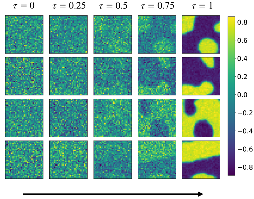
Figure 4: The denoising process for generating four independent configurations from a well-trained diffusion model.

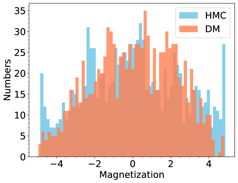
Figure 5: Comparison of the distribution of the magnetization with 1024 samples generated from the well-trained diffusion model and using HMC.

4.3 Symmetric Phase

We now turn to the symmetric phase and take $\kappa=0.21$, below but near the critical value. In the thermodynamic limit, the phase transition can be characterized by a divergence in the connected two-point susceptibility. This susceptibility is a measure of how a system responds to small perturbations and is defined as

$$\chi_{2}=V\left(\langle M^{2}\rangle-\langle M\rangle^{2}\right).$$ (36)

In addition, the Binder cumulant Binder:1981zz is a dimensionless quantity often used to identify phase transitions, defined as a ratio of moments of a distribution,

$$U_{L}=1-\frac{1}{3}\frac{\langle M^{4}\rangle}{\langle M^{2}\rangle^{2}}.$$ (37)

It is sensitive to the shape of the distribution, i.e., the kurtosis of the order parameter, and is particularly useful for detecting and analyzing phase transitions in finite-size systems.

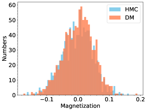
Figure 6: Comparison of the distribution of the magnetization in the symmetric phase from the test data-set (HMC) and from the well-trained diffusion model (DM). The number of independent configurations is 1024 in both cases.

data-set	$\langle M\rangle$	$\chi_{2}$	$U_{L}$
Training (HMC)	0.0012$\pm$ 0.0007	2.5160 $\pm$ 0.0457	0.1042 $\pm$ 0.0367
Testing (HMC)	0.0018 $\pm$ 0.0015	2.4463 $\pm$ 0.1099	-0.0198 $\pm$ 0.1035
Generated (DM)	0.0017$\pm$ 0.0015	2.4227 $\pm$ 0.1035	0.0484 $\pm$ 0.0959

Table 1: Comparison of observables calculated on different datasets with lower error bounds determined using the statistical jackknife method. The sample size is comparable for the bottom two rows and a factor of 5 larger for the training set (top row).

In Fig. 6 we compare the distributions of the magnetization obtained independently from the trained DM and using HMC. Good consistency between the distributions is observed. To make this more quantitative we present in Table 1 the magnetization $\langle M\rangle$, two-point susceptibility $\chi_{2}$, and the Binder cumulant $U_{L}$ obtained using both the trained diffusion model and with HMC. For the latter, expectation values are shown both for the training set and the testing set, with the former having a factor of five more configurations, which is reflected in the uncertainty. We conclude that the diffusion model is capable of accurately capturing the statistical properties of the system, as reflected by these observables, and is in good agreement with HMC, a well-established method for sampling from the target distribution. We note that no accept-reject step has been applied in the diffusion model.

4.3.1 Unsupervised Action Estimation

The likelihood computation method described in Section 3.3 enables us to estimate the action for the field configurations generated by the trained diffusion model. By comparing the action estimation from the trained DMs with the true action, see Eq. (32), we can confirm whether the DM has captured the underlying physics correctly.

For this purpose, we first generate an ensemble of field configurations using the trained DM. We then compute the likelihoods, $q(\phi)$, for these configurations using the probability flow ODE approach. By applying the change-of-variable formula, we are able to compute the action values for these field configurations, as

$$S_{\text{eff}}=-\log q(\phi),$$ (38)

where the constant term $Z$ has been omitted. In Fig. 7 we compare the evaluated effective action with the one obtained directly from the physical action, i.e., Eq. (32). The black dashed line means the $x-$axis is proportional to the $y-$axis, and the green sites are action values estimated from the probabilistic ODE (on the $x-$axis) and calculated from the physical action (on the $y-$axis).

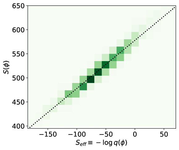
Figure 7: Correlation between the effective action estimated from the trained DM using the probabilistic ODE and from the physical action on 1024 samples.

The coefficient of determination, $R^{2}$, is a useful metric for quantitatively measuring how well the estimated action values, denoted as $S_{\rm eff}(\phi_{i})$, match the actual ones, denoted as $S(\phi_{i})$. Here $i$ indicates the index in sampled configurations. We use

$$R^{2}=1-\frac{\sum_{i}\left[S(\phi_{i})-S_{\text{eff}}(\phi_{i})\right]^{2}}{\sum_{i}\left[S(\phi_{i})-\overline{S}(\phi)\right]},$$ (39)

where $\overline{S}(\phi)$ is the average value for the actual action,

$$\overline{S}(\phi)=\frac{1}{N}\sum_{i=1}^{N}S(\phi_{i}).$$ (40)

It measures the proportion of variation in the dependent variable (in this case, the action) that is predictable from the independent variable (in this case, the diffusion model-generated samples). $R^{2}$ values close to 1 indicate that the diffusion model provides an accurate estimate of the action, suggesting that the trained diffusion model has effectively learned the underlying physics of the scalar field theory correctly. In Fig. 7, with the default dataset size, i.e., 5120 samples for training, the $R^{2}$ value is 0.960 calculated on the 1024 generated configurations.

4.3.2 Autocorrelation Time

Critical slowing down Wolff:1989wq emerges when simulations approach a critical point and the correlation length of the system diverges. This can be studied using the autocorrelation function of an observable $O$, defined as

$$C_{O}(t)=\left\langle(O_{t_{0}}-\left\langle O_{t_{0}}\right\rangle)(O_{t_{0}+t}-\left\langle O_{t_{0}+t}\right\rangle)\right\rangle=\left\langle O_{t_{0}}O_{t_{0}+t}\right\rangle-\left\langle O_{t_{0}}\right\rangle\left\langle O_{t_{0}+t}\right\rangle,$$ (41)

where $t_{0}$ is the starting time and $t$ denotes the time along the Markov chain. In an exponential fit, $C_{O}(t)\sim\exp\{-t/t_{c}\}$, the characteristic time $t_{c}$ should scale as a power of the correlation length $\xi$ around the critical point, i.e., $t_{c}\sim\xi^{z}$ (the correlation length $\xi$ should not be confused with the time variable in the forward SDE).

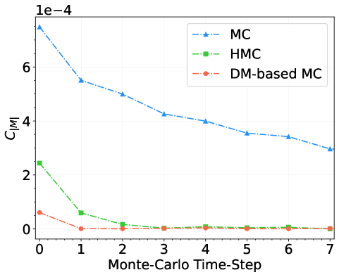
Figure 8: Comparison of the autocorrelation function of $|M|$ for the Metropolis-Hastings MC algorithm, HMC, and DM-based MC, using 1024 samples.

We investigate this for the “absolute value” of the magnetization, defined as

$$|M|=\frac{1}{V}\left\langle\sum_{x}\left|\phi(x)\right|\right\rangle,$$ (42)

and compare various updates. Because the likelihood of samples can be computed, as shown in the previous section, we can use the Metropolis-Hastings (MH) algorithm to construct the asymptotically exact Markov chain sampler with the well-trained diffusion model. We refer to this as the DM-based Monte-Carlo method, following the convention of flow-based models. The acceptance criterion is corrected as

$$p_{\text{accept}}(\phi_{\text{proposal}}\mid\phi^{i-1})=\text{min}\left(1,\frac{q(\phi^{i-1})}{p(\phi^{i-1})}\frac{q(\phi_{\text{proposal}})}{p(\phi_{\text{proposal}})}\right),$$ (43)

where $\phi^{i-1}$ is the previous configuration and $\phi_{\text{proposal}}$ is sampled from the well-trained DM. Further, we can estimate the efficiency gain of the DM by comparing the behavior of the autocorrelation function $C_{|M|}(t)$ with the one obtained using a Metropolis-Hastings Monte-Carlo (MC) and the HMC algorithm on 1024 configurations, as shown in Fig. 8. This demonstrates that our proposed method has the potential to significantly suppress autocorrelations along a Markov chain.

5 Conclusion and Outlook

In this work, we proposed a new method to generate quantum field configurations using diffusion models (DMs), popular in the ML community. We highlighted the connection with stochastic quantization (SQ), an approach to quantize field theories based on a stochastic process in a fictitious time direction. In SQ the drift term in the stochastic process is known, as it is derived from the probability distribution one wants to sample from, which is determined by the quantum theory under consideration. In DMs the drift term is not known but is learned from data in a forward stochastic process. After estimating the drift term, the trained DM is run in the opposite direction and independent configurations are created from noise, the “denoising” process. This latter part is akin to the dynamics in SQ, albeit with a learned and time-dependent drift term.

We have demonstrated the approach in a simple toy model and in a two-dimensional scalar field theory with a $\phi^{4}$ interaction, both in the symmetric and in the broken phase. We have shown that the DM can serve as a global sampler to assist methods based on the Monte Carlo principle. We note that one can include an accept-reject step at the end of each trajectory. We have found in our numerical results that the well-trained DM can successfully reproduce configurations in both phases and that autocorrelation times are reduced along a Markov chain. This improvement in sampling efficiency can be beneficial for studying lattice field theories and should be analyzed further.

There are various directions to explore in the future. The forward (“smoothening”) and backward (“denoising”) processes are reminiscent of (inverse) renormalization group transformations and it would be interesting to make this precise. Because the action can be estimated relatively accurately, it is feasible to train a DM without preparing a training data-set, which needs to be investigated. The connection between DMs and SQ offers new perspectives. It is well known how to implement SQ for non-abelian gauge theories; hence it should be possible to formulate DMs for the non-abelian case. An intriguing direction is the following: imagine one has generated a set of configurations for a quantum field theory with fermions, such as QCD or the Schwinger model. Since the fermions are “integrated out”, the configurations are given in terms of the gauge fields only. By using these configurations as the starting point of a DM, one can learn an effective stochastic process which incorporates the effect of the fermions implicitly. This may be used to create additional configurations in a numerically “cheap” manner. An accept-reject step based on the underlying theory can be included, which would require the evaluation of the fermion determinant. Finally SQ can also be used for theories with a sign or complex action problem, and hence a non-positive definite distribution. This is commonly known as complex Langevin (CL) dynamics. It is known that CL may become less reliable along long trajectories in the stochastic process. Combining CL with DMs, one may consider fairly short trajectories, but subsequently use the resulting configurations to train the DM to generate additional configurations to increase statistics.

Note added.

Recent related work introduces the stochastic process into the hybrid Monte-Carlo algorithm Robnik:2023pgt and explores the correspondence between the exact renormalizing group (ERG) and diffusion models based upon heat equation Cotler:2023lem .

Appendix A U-Net Architecture

U-Net architecture is utilized to present $s_{\mathbf{\theta}}(\phi,t)$ with a time-embedding input. This architecture is widely used in tasks that require semantic segmentation due to its ability to capture both local and global information in an image. The model is initialized with a function that calculates the standard deviation of the perturbation kernel, a list of channels for feature maps at each resolution, and an embedding dimension for Gaussian random feature embeddings. The model consists of an encoding path (contracting path) and a decoding path (expansive path), which are characteristic of the U-Net architecture, as Fig. 9 shown.

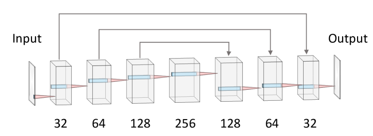
Figure 9: Sketch of the U-Net Architecture, where the gray lines with arrows indicate skip connections between encoding paths and decoding paths. In this study, the default shape of the input is set as $(\cdot,1,32,32)$, where the first dimension is the batch size, the second indicates the channel, and the final two represent dimensionalities of the field configuration.

The encoding path consists of four convolutional layers (conv1 to conv4), each followed by a dense layer (dense1 to dense4), and a group normalization layer (gnorm1 to gnorm4). The convolutional layers progressively increase the number of channels from 1 to 32, 64, 128, 256. The dense layers incorporate information from the time embedding into the feature maps, and the group normalization layers normalize the feature maps across the channels.

The decoding path consists of four transposed convolutional layers (tconv4 to tconv1), each followed by a dense layer (dense5 to dense7), and a group normalization layer (tgnorm4 to tgnorm2). The transposed convolutional layers progressively decrease the number of channels back to 1. The dense layers incorporate information from the time embedding into the feature maps, and the group normalization layers normalize the feature maps across the channels. The decoding path also includes skip connections from the encoding path, which help the model to better localize and learn representations with less loss of spatial information.

The model uses the Swish activation function, which is a smooth, non-monotonic function that has been found to work better than ReLU in deeper models. In the forward pass, the model first obtains the Gaussian random feature embedding for the input time $t$. It then passes the input $\phi$ through the encoding path, where it applies the convolutional, dense, group normalization, and activation layers sequentially. It then passes the output of the encoding path through the decoding path, where it applies the transposed convolutional, dense, group normalization, and activation layers sequentially, while also adding the skip connections from the encoding path. Finally, it normalizes the output by the standard deviation of the perturbation kernel at time $t$ and returns it.

Appendix B Skilling-Hutchinson Estimator

In practice, the divergence function in Eq. (25) can be hard to evaluate for general vector-valued functions $f$, but we can use an unbiased estimator, named Skilling-Hutchinson estimator grathwohl2018scalable , to approximate the trace. Let $\bm{\epsilon}\sim\mathcal{N}(\mathbf{0},\mathbf{I})$. The Skilling-Hutchinson estimator is based on the fact that

$$\mathbf{\nabla}\cdot f(\phi)=\mathbb{E}_{\bm{\epsilon}\sim\mathcal{N}(\mathbf{0},\mathbf{I})}\left[\bm{\epsilon}^{\intercal}J_{f}(\phi)\bm{\epsilon}\right].$$ (44)

Therefore, we can simply sample a random vector $\bm{\epsilon}\sim\mathcal{N}(\mathbf{0},\mathbf{I})$, and then use $\bm{\epsilon}^{\intercal}J_{f}(\phi)\bm{\epsilon}$ to estimate the divergence of $f(\phi)$. This estimator only requires computing the Jacobian-vector product $J_{f}(\phi)\bm{\epsilon}$, which is typically efficient.

As a result, for our probability flow ODE, we can compute the (log) data likelihood with the following

$$\log p_{0}(\phi(0))=\log p_{1}(\phi(1))-\int_{0}^{1}\frac{d[\sigma^{2}(t)]}{dt}\mathbf{\nabla}\cdot s_{\theta}(\phi(t),t)dt.$$ (45)

With the Skilling-Hutchinson estimator, we can compute the divergence via

$$\mathbf{\nabla}\cdot s_{\theta}(\phi(t),t)=\mathbb{E}_{\bm{\epsilon}\sim\mathcal{N}(\mathbf{0},\mathbf{I})}\left[\bm{\epsilon}^{\intercal}J_{s_{\theta}}(\phi(t),t)\bm{\epsilon}\right].$$ (46)

Subsequently, we can compute the integral using numerical integrators. This provides us with an unbiased estimate of the true likelihood of the data, and we can make this estimate increasingly accurate by running the calculation multiple times and taking the average. The numerical integrator requires $\phi(t)$ as a function of $t$, which can be obtained by the probability flow ODE sampler. In our calculations, we tested different sampling sizes ranging from 1 to 100 and found that it converges when the size is larger than 10. Therefore, we chose the sample size $\bm{\epsilon}$ as 10 to ensure the accuracy of the estimation.

References

- (1) F. Knechtli, M. Günther and M. Peardon, Lattice Quantum Chromodynamics: Practical Essentials, SpringerBriefs in Physics, Springer (2017), 10.1007/978-94-024-0999-4.
- (2) U. Wolff, CRITICAL SLOWING DOWN, Nucl. Phys. B Proc. Suppl. 17 (1990) 93.
- (3) J.M. Tomczak, Deep Generative Modeling, Springer International Publishing, Cham (2022), 10.1007/978-3-030-93158-2.
- (4) D. Boyda et al., Applications of Machine Learning to Lattice Quantum Field Theory, in Snowmass 2021, 2, 2022 [2202.05838].
- (5) K. Zhou, G. Endrődi, L.-G. Pang and H. Stöcker, Regressive and generative neural networks for scalar field theory, Phys. Rev. D 100 (2019) 011501.
- (6) J.M. Pawlowski and J.M. Urban, Reducing autocorrelation times in lattice simulations with generative adversarial networks, Mach. Learn.: Sci. Technol. 1 (2020) 045011.
- (7) M.S. Albergo, G. Kanwar and P.E. Shanahan, Flow-based generative models for Markov chain Monte Carlo in lattice field theory, Phys. Rev. D 100 (2019) 034515 [1904.12072].
- (8) G. Kanwar, M.S. Albergo, D. Boyda, K. Cranmer, D.C. Hackett, S. Racanière et al., Equivariant Flow-Based Sampling for Lattice Gauge Theory, Phys. Rev. Lett. 125 (2020) 121601 [2003.06413].
- (9) K.A. Nicoli, C.J. Anders, L. Funcke, T. Hartung, K. Jansen, P. Kessel et al., Estimation of Thermodynamic Observables in Lattice Field Theories with Deep Generative Models, Phys. Rev. Lett. 126 (2021) 032001 [2007.07115].
- (10) M.S. Albergo, G. Kanwar, S. Racanière, D.J. Rezende, J.M. Urban, D. Boyda et al., Flow-based sampling for fermionic lattice field theories, Phys. Rev. D 104 (2021) 114507 [2106.05934].
- (11) M.S. Albergo, D. Boyda, D.C. Hackett, G. Kanwar, K. Cranmer, S. Racanière et al., Introduction to Normalizing Flows for Lattice Field Theory, arXiv:2101.08176 [hep-lat] (2021) [2101.08176].
- (12) L. Del Debbio, J. Marsh Rossney and M. Wilson, Efficient modeling of trivializing maps for lattice theory using normalizing flows: A first look at scalability, Phys. Rev. D 104 (2021) 094507 [2105.12481].
- (13) D.C. Hackett, C.-C. Hsieh, M.S. Albergo, D. Boyda, J.-W. Chen, K.-F. Chen et al., Flow-based sampling for multimodal distributions in lattice field theory, 2107.00734.
- (14) M.S. Albergo, D. Boyda, K. Cranmer, D.C. Hackett, G. Kanwar, S. Racanière et al., Flow-based sampling in the lattice Schwinger model at criticality, Phys. Rev. D 106 (2022) 014514 [2202.11712].
- (15) S. Bacchio, P. Kessel, S. Schaefer and L. Vaitl, Learning Trivializing Gradient Flows for Lattice Gauge Theories, Phys. Rev. D 107 (2023) L051504 [2212.08469].
- (16) M. Caselle, E. Cellini, A. Nada and M. Panero, Stochastic normalizing flows as non-equilibrium transformations, JHEP 07 (2022) 015 [2201.08862].
- (17) S. Chen, O. Savchuk, S. Zheng, B. Chen, H. Stoecker, L. Wang et al., Fourier-flow model generating Feynman paths, Phys. Rev. D 107 (2023) 056001 [2211.03470].
- (18) M. Gerdes, P. de Haan, C. Rainone, R. Bondesan and M.C.N. Cheng, Learning Lattice Quantum Field Theories with Equivariant Continuous Flows, 2207.00283.
- (19) D. Albandea, L. Del Debbio, P. Hernández, R. Kenway, J. Marsh Rossney and A. Ramos, Learning trivializing flows, Eur. Phys. J. C 83 (2023) 676 [2302.08408].
- (20) A. Singha, D. Chakrabarti and V. Arora, Conditional normalizing flow for Markov chain Monte Carlo sampling in the critical region of lattice field theory, Phys. Rev. D 107 (2023) 014512.
- (21) R. Abbott et al., Aspects of scaling and scalability for flow-based sampling of lattice QCD, 2211.07541.
- (22) K.A. Nicoli, C.J. Anders, T. Hartung, K. Jansen, P. Kessel and S. Nakajima, Detecting and Mitigating Mode-Collapse for Flow-based Sampling of Lattice Field Theories, 2302.14082.
- (23) L. Wang, Y. Jiang, L. He and K. Zhou, Continuous-Mixture Autoregressive Networks Learning the Kosterlitz-Thouless Transition, Chin. Phys. Lett. 39 (2022) 120502 [2005.04857].
- (24) D. Luo, Z. Chen, K. Hu, Z. Zhao, V.M. Hur and B.K. Clark, Gauge-invariant and anyonic-symmetric autoregressive neural network for quantum lattice models, Phys. Rev. Res. 5 (2023) 013216.
- (25) M. Favoni, A. Ipp, D.I. Müller and D. Schuh, Lattice Gauge Equivariant Convolutional Neural Networks, Phys. Rev. Lett. 128 (2022) 032003 [2012.12901].
- (26) J. Aronsson, D.I. Müller and D. Schuh, Geometrical aspects of lattice gauge equivariant convolutional neural networks, 2303.11448.
- (27) R. Abbott, M.S. Albergo, D. Boyda, K. Cranmer, D.C. Hackett, G. Kanwar et al., Gauge-equivariant flow models for sampling in lattice field theories with pseudofermions, Phys. Rev. D 106 (2022) 074506 [2207.08945].
- (28) K. Zhou, L. Wang, L.-G. Pang and S. Shi, Exploring QCD matter in extreme conditions with Machine Learning, 2303.15136.
- (29) W.-B. He, Y.-G. Ma, L.-G. Pang, H.-C. Song and K. Zhou, High-energy nuclear physics meets machine learning, Nucl. Sci. Tech. 34 (2023) 88 [2303.06752].
- (30) L. Yang, Z. Zhang, S. Hong, R. Xu, Y. Zhao, Y. Shao et al., Diffusion Models: A Comprehensive Survey of Methods and Applications, Sept., 2022. 10.48550/arXiv.2209.00796.
- (31) F.-A. Croitoru, V. Hondru, R.T. Ionescu and M. Shah, Diffusion models in vision: A survey, IEEE Transactions on Pattern Analysis and Machine Intelligence (2023) 1.
- (32) A. Ramesh, P. Dhariwal, A. Nichol, C. Chu and M. Chen, Hierarchical Text-Conditional Image Generation with CLIP Latents, arXiv e-prints (2022) [2204.06125].
- (33) R. Rombach, A. Blattmann, D. Lorenz, P. Esser and B. Ommer, High-resolution image synthesis with latent diffusion models, in Proceedings of the IEEE/CVF Conference on Computer Vision and Pattern Recognition (CVPR), pp. 10684–10695, June, 2022.
- (34) V. Mikuni and B. Nachman, Score-based generative models for calorimeter shower simulation, Phys. Rev. D 106 (2022) 092009 [2206.11898].
- (35) V. Mikuni, B. Nachman and M. Pettee, Fast point cloud generation with diffusion models in high energy physics, Phys. Rev. D 108 (2023) 036025 [2304.01266].
- (36) G. Parisi and Y.S. Wu, Perturbation theory without gauge fixing, Sci. China, A 24 (1980) 483.
- (37) P.H. Damgaard and H. Hüffel, Stochastic quantization, Phys. Rept. 152 (1987) 227.
- (38) M. Namiki, Basic ideas of stochastic quantization, Prog. Theor. Phys. Suppl. 111 (1993) 1.
- (39) G. Parisi, On complex probabilities, Physics Letters B 131 (1983) 393.
- (40) J. Berges, S. Borsanyi, D. Sexty and I.O. Stamatescu, Lattice simulations of real-time quantum fields, Phys. Rev. D 75 (2007) 045007 [hep-lat/0609058].
- (41) G. Aarts and I.-O. Stamatescu, Stochastic quantization at finite chemical potential, JHEP 09 (2008) 018 [0807.1597].
- (42) G. Aarts, Can stochastic quantization evade the sign problem? The relativistic Bose gas at finite chemical potential, Phys. Rev. Lett. 102 (2009) 131601 [0810.2089].
- (43) E. Seiler, D. Sexty and I.-O. Stamatescu, Gauge cooling in complex Langevin for QCD with heavy quarks, Phys. Lett. B 723 (2013) 213 [1211.3709].
- (44) D. Sexty, Simulating full QCD at nonzero density using the complex Langevin equation, Phys. Lett. B 729 (2014) 108 [1307.7748].
- (45) G. Aarts, Introductory lectures on lattice QCD at nonzero baryon number, J. Phys. Conf. Ser. 706 (2016) 022004 [1512.05145].
- (46) F. Attanasio, B. Jäger and F.P.G. Ziegler, Complex Langevin simulations and the QCD phase diagram: Recent developments, Eur. Phys. J. A 56 (2020) 251 [2006.00476].
- (47) C.E. Berger, L. Rammelmüller, A.C. Loheac, F. Ehmann, J. Braun and J.E. Drut, Complex Langevin and other approaches to the sign problem in quantum many-body physics, Phys. Rept. 892 (2021) 1 [1907.10183].
- (48) K. Nagata, Finite-density lattice QCD and sign problem: Current status and open problems, Prog. Part. Nucl. Phys. 127 (2022) 103991 [2108.12423].
- (49) G. Aarts, E. Seiler and I.-O. Stamatescu, Complex Langevin method: When can it be trusted?, Phys. Rev. D 81 (2010) 054508.
- (50) G. Aarts, F.A. James, E. Seiler and I.-O. Stamatescu, Complex Langevin: Etiology and Diagnostics of its Main Problem, Eur. Phys. J. C 71 (2011) 1756 [1101.3270].
- (51) K. Nagata, J. Nishimura and S. Shimasaki, Argument for justification of the complex Langevin method and the condition for correct convergence, Phys. Rev. D 94 (2016) 114515.
- (52) G. Aarts, E. Seiler, D. Sexty and I.-O. Stamatescu, Complex Langevin dynamics and zeroes of the fermion determinant, JHEP 05 (2017) 044 [1701.02322].
- (53) M. Scherzer, E. Seiler, D. Sexty and I.-O. Stamatescu, Complex Langevin and boundary terms, Phys. Rev. D 99 (2019) 014512 [1808.05187].
- (54) M. Westh Hansen and D. Sexty, Complex Langevin boundary terms in full QCD, PoS LATTICE2022 (2023) 163 [2212.12029].
- (55) D. Alvestad, R. Larsen and A. Rothkopf, Stable solvers for real-time Complex Langevin, JHEP 08 (2021) 138 [2105.02735].
- (56) D. Alvestad, R. Larsen and A. Rothkopf, Towards learning optimized kernels for complex Langevin, JHEP 04 (2023) 057 [2211.15625].
- (57) N.M. Lampl and D. Sexty, Real time evolution of scalar fields with kernelled Complex Langevin equation, 2309.06103.
- (58) D.J.E. Callaway and A. Rahman, The Microcanonical Ensemble: A New Formulation of Lattice Gauge Theory, Phys. Rev. Lett. 49 (1982) 613.
- (59) H. Risken, The Fokker-Planck equation: Methods of solution and application, Springer (1996).
- (60) M. Namiki, I. Ohba, K. Okano, Y. Yamanaka, A.K. Kapoor, H. Nakazato et al., Stochastic quantization, vol. 9, Springer Berlin Heidelberg (1992), 10.1007/978-3-540-47217-9.
- (61) G.G. Batrouni, G.R. Katz, A.S. Kronfeld, G.P. Lepage, B. Svetitsky and K.G. Wilson, Langevin Simulations of Lattice Field Theories, Phys. Rev. D 32 (1985) 2736.
- (62) J. Sohl-Dickstein, E.A. Weiss, N. Maheswaranathan and S. Ganguli, Deep unsupervised learning using nonequilibrium thermodynamics, in Proc. 32nd Int. Conf. Int. Conf. Mach. Learn. - Vol. 37, ICML’15, (Lille, France), pp. 2256–2265, JMLR.org, July, 2015.
- (63) Y. Song and S. Ermon, Generative modeling by estimating gradients of the data distribution, in Adv. Neural Inf. Process. Syst., H. Wallach, H. Larochelle, A. Beygelzimer, F. dAlché-Buc, E. Fox and R. Garnett, eds., vol. 32, Curran Associates, Inc., 2019.
- (64) Y. Song, J. Sohl-Dickstein, D.P. Kingma, A. Kumar, S. Ermon and B. Poole, Score-based generative modeling through stochastic differential equations, in Int. Conf. Learn. Represent., 2021.
- (65) J. Ho, A. Jain and P. Abbeel, Denoising diffusion probabilistic models, in Proc. 34th Int. Conf. Neural Inf. Process. Syst., NIPS’20, (Red Hook, NY, USA), pp. 6840–6851, Curran Associates Inc., Dec., 2020.
- (66) B.D.O. Anderson, Reverse-time diffusion equation models, Stochastic Processes and their Applications 12 (1982) 313.
- (67) A. Hyvärinen, Estimation of non-normalized statistical models by score matching, Journal of Machine Learning Research 6 (2005) 695.
- (68) P. Vincent, A connection between score matching and denoising autoencoders, Neural Computation 23 (2011) 1661.
- (69) M. Welling and Y.W. Teh, Bayesian learning via stochastic gradient langevin dynamics, in Proc. 28th Int. Conf. Int. Conf. Mach. Learn., ICML’11, (Madison, WI, USA), pp. 681–688, Omnipress, June, 2011.
- (70) D. Maoutsa, S. Reich and M. Opper, Interacting particle solutions of fokker–planck equations through gradient–log–density estimation, Entropy 22 (2020) .
- (71) W. Grathwohl, R.T.Q. Chen, J. Bettencourt and D. Duvenaud, Scalable reversible generative models with free-form continuous dynamics, in International Conference on Learning Representations, 2019.
- (72) M. Luscher, Trivializing maps, the Wilson flow and the HMC algorithm, Commun. Math. Phys. 293 (2010) 899 [0907.5491].
- (73) Z. Bern, M.B. Halpern and L. Sadun, Continuum Regularization of Quantum Field Theory. 4. Langevin Renormalization, Z. Phys. C 35 (1987) 255.
- (74) J.M. Pawlowski, I.-O. Stamatescu and F.P.G. Ziegler, Cooling stochastic quantization with colored noise, Phys. Rev. D 96 (2017) 114505.
- (75) J. Smit, Introduction to quantum fields on a lattice: A robust mate, vol. 15, Cambridge University Press (1, 2011).
- (76) S. Akiyama, Y. Kuramashi and Y. Yoshimura, Phase transition of four-dimensional lattice theory with tensor renormalization group, Phys. Rev. D 104 (2021) 034507 [2101.06953].
- (77) R.M. Neal et al., Mcmc using hamiltonian dynamics, Handbook of markov chain monte carlo 2 (2011) 2.
- (78) O. Ronneberger, P. Fischer and T. Brox, U-net: Convolutional networks for biomedical image segmentation, in Medical Image Computing and Computer-Assisted Intervention – MICCAI 2015, N. Navab, J. Hornegger, W.M. Wells and A.F. Frangi, eds., (Cham), pp. 234–241, Springer International Publishing, 2015.
- (79) K. Binder, Critical Properties from Monte Carlo Coarse Graining and Renormalization, Phys. Rev. Lett. 47 (1981) 693.
- (80) J. Robnik and U. Seljak, Microcanonical Langevin Monte Carlo, 2303.18221.
- (81) J. Cotler and S. Rezchikov, Renormalizing Diffusion Models, 2308.12355.