ComPACT: combined ACT+Planck galaxy cluster catalogue

Abstract

Galaxy clusters are the most massive gravitationally bound systems consisting of dark matter, hot baryonic gas and stars. They play an important role in observational cosmology and galaxy evolution studies. We have developed a deep learning model for segmentation of SZ signal on ACT+Planck intensity maps and present here a new galaxy cluster catalogue in the ACT footprint. In order to increase the purity of the cluster catalogue, we limit ourselves to publishing here only a part of the full sample with the most probable galaxy clusters lying in the directions to the candidates of the extended Planck cluster catalogue (SZcat). The ComPACT catalogue contains 2,934 galaxy clusters (with $Purity\gtrsim 88$%), $\gtrsim 1436$ clusters are new with respect to the existing ACT DR5 and PSZ2 cluster samples.

1 Introduction

Galaxy clusters are the most massive gravitationally bound systems in the Universe (see Allen et al., 2011; Kravtsov & Borgani, 2012, for reviews). These objects are located at the nodes of the cosmic web and serve as reliable tracers of the underlying dark matter distribution. The cluster mass function, which describes the number density of galaxy clusters as a function of their mass, and its evolution with redshift provide a critical test of structure formation models and allows to constrain cosmological parameters (e.g. Vikhlinin et al., 2009; Pratt et al., 2019; Burenin & Vikhlinin, 2012; Mantz et al., 2015, among others).

Galaxy clusters are composed of dark matter, which makes up around 85% of their total mass, the intracluster medium (ICM; $\sim$ 12% of the total mass), which is an ionised hot gas, and stars ($\sim$ 3%). Consequently, they can be detected at several wavelength bands. In the optical range, galaxy clusters represent a concentration of elliptical galaxies. Clusters are also bright in X-rays due to the bremsstrahlung emission produced by the ionised ICM (Sarazin, 1988). X-ray catalogues may provide a wealth of information about galaxy clusters, such as their temperature, luminosity, and gas mass, which are essential for understanding the formation and evolution of these structures. The same hot ICM (namely, the high-energy electrons) also interacts with low-energy cosmic microwave background (CMB) radiation through the inverse Compton scattering creating a distortion in the black-body spectrum (the thermal Sunyaev-Zeldovich effect; Sunyaev & Zeldovich (1970, 1972)). The ICM boosts CMB photons to higher frequencies resulting in a characteristic increase/decrease in the CMB intensity depending on the specific microwave frequency in which a galaxy cluster is being observed. Studying galaxy clusters in (sub)millimetre range via the SZ effect has several advantages over other wavelength ranges. First, the magnitude of the SZ effect does not depend on redshift, thus providing a powerful tool for detecting clusters at high redshifts. Second, the SZ signal is proportional to the integrated gas pressure along the line of sight through the cluster, which is directly linked to the total mass of a cluster. The relationship between the integrated Compton parameter $Y_{SZ}$ (the total SZ flux) and a cluster mass $M$ has already proved to be particularly tight (see Kravtsov et al., 2006; Planck Collaboration et al., 2013, among many others). The number of SZ catalogues have been released in recent years including the Planck survey (Planck Collaboration (2014); Planck Collaboration (2016)), the South pole telescope (SPT, Bleem et al. (2015) and the Atacama Cosmology Telescope (ACT; Hilton, M. et al. (2021)). With ongoing and upcoming CMB surveys, more than $10^{4}$ galaxy clusters are expected to be detected (Raghunathan et al., 2022). Together with reliable mass estimates, such cluster samples may have a ground-breaking impact on our understanding of the structure growth in the Universe, the dark energy equation of state, and modified gravity theories (e.g. Bocquet et al., 2015; Planck Collaboration et al., 2016a; Burenin & Vikhlinin, 2012; Mantz et al., 2015; Burenin, 2018, 2013) .

Recently, Meshcheryakov et al. (2022) presented SZcat – a catalogue of Planck extended SZ sources with a low level of significance (so that nearly all possible Planck cluster candidates are there along with a large number of spurious detections). Here, we aim to develop a method for an automated cluster detection on publicly available combined ACT and Planck maps (Naess et al., 2020) and to apply it to the fields of SZcat sources. As a result, we obtain a new catalogue of galaxy clusters – ComPACT – characterised by high purity.

The paper is organised as follows. In the next section we review deep learning models for SZ clusters detection proposed in literature. Section 2 describes data used in this work. In Section 3, we describe a deep learning model for cluster segmentation and a procedure for an object detection. Then, in Section 4 the ComPACT catalogue is described. In Section 5 our conclusions are presented.

1.1 Deep learning models for SZ clusters detection

In the last few years, deep learning approaches were successfully applied to various object detection and segmentation problems in observational astronomy in different spectral domains: e.g. to imaging data in radio (Hartley et al., 2023), microwave (Meshcheryakov et al., 2022; Lin et al., 2021; Bonjean, 2020), and optical (Burke et al., 2019) spectral ranges. The key advantages of deep learning models over classical astronomical object detection methods (such as SExtractor (Bertin & Arnouts, 1996) in the optical or Matched Multi-filter approach (Melin, J.-B. et al., 2006) in the microwave) are: (i) unification of an object detection model architecture over many spectral domains, and (ii) the amazing ability of a DL method to improve itself with the increase of size of available training sample. As it was shown in SKA Science Data Challenge 2 (Hartley et al., 2023), deep learning models trained on a large and representative enough knowledge base outperform a classical approaches in the astronomical object detection tasks.

As mentioned above, DL approaches were successfully applied to microwave imaging data. Bonjean (2020) proposed to use a DL model with the U-Net architecture to make a segmentation map of SZ signal from raw Planck HFI imaging data and detected SZ sources on it. Verkhodanov et al. (2021) trained a CNN classification model to recognise SZ sources in Planck intensity maps. Lin et al. (2021) proposed a hybrid model (DeepSZ, based on a combination of CNN and a classical MMF approach) and demonstrated its power in detecting SZ sources using the simulated CMB maps (with characteristics similar to SPT-3G survey).

In all papers mentioned above no catalogue of SZ sources was presented. Recently, Meshcheryakov et al. (2022) trained a U-Net model on Planck HFI data and presented SZcat – a full catalogue of cluster candidates. SZcat contains potential SZ sources over the whole extragalactic sky obtained by two methods: (a) using the DL model (described in Meshcheryakov et al. (2022)) and applying it to Planck HFI intensity maps; and by (b) using a classical detection approach (Burenin, 2017) and applying it to Compton parameter maps published in Planck 2015 data release (Planck Collaboration et al., 2016b). SZcat contains SZ sources detected down to low significance values. It is supposed to have the highest completeness level for clusters seen in Planck, but low purity of candidates in the full catalogue. In order to increase a purity of SZcat (staying at the high completeness level), one needs to combine SZcat with other cluster catalogues or with data from different instrument(s) (e.g. SPT, ACT) in the same microwave spectral domain, or with cluster data obtained in different spectral range (optical-IR, X-ray).

Using a combination of data from different telescopes makes it possible to lower the threshold for cluster detection, so that new objects can be found with high precision. Melin, J.-B. et al. (2021) combined Planck and SPT microwave data; Tarrío, P. et al. (2019) combined Planck data with ROSAT X-ray catalogue. In both cases of Planck-SPT and Planck-ROSAT data combination, new cluster catalogues were published (with higher completeness/purity than cluster catalogues obtained from Planck/SPT/ROSAT data individually).

2 Data

We use publicly available composite ACT+Planck intensity maps from Naess et al. (2020) at 98, 150, and 220 GHz with 0.5 arcmin per pix resolution covering around 18,000 squared degrees of the sky area (which we call as the ACT footprint hereafter).

In order to train and test a SZ cluster segmentation model (see Section 3) we use the following catalogues of galaxy clusters and radio sources found in ACT data:

• the ACT DR5 cluster catalogue (Hilton, M. et al., 2021), which contains 4,195 optically confirmed galaxy clusters. The sources were selected by using the multi-frequency matched filter method (MMF, Melin, J.-B. et al. (2006); Williamson et al. (2011)) from the ACT multi-frequency data collected from 2008 to 2018;

• a catalogue of point sources (predominantly, active galactic nuclei) from Datta et al. (2019), which covers 680 squared degrees of the full ACT footprint;

• the equatorial catalogue of extragalactic sources (Gralla et al., 2020), which contains 287 dusty star-forming galaxies and 510 radio-loud active galactic nuclei (AGN).

Also we use external X-ray and SZ cluster catalogues: MCXC, 4XMM DR12, SPT-SZ, ComPRASS, and PSZSPT (see Appendix B).

3 Method

Fig. 1 illustrates the sequence of pipeline steps in constructing a catalogue of potential SZ sources. We convert the full ACT+Planck intensity map into a SZ signal segmentation map by using a Deep Learning classification model (see Section3.1). Then, the detection procedure (described in Section3.2) is applied to the SZ signal segmentation map, resulting in a catalogue of SZ sources candidates. Below, we describe the SZ signal segmentation and source detection procedures in detail.

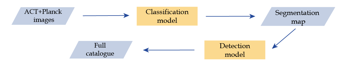
Figure 1: Scheme showing main steps of building the catalogue of potential SZ sources

3.1 Deep learning SZ signal segmentation model

To recognise SZ signal on ACT+Planck intensity maps, one could follow the approach already presented in Meshcheryakov et al. (2022); Bonjean (2020), i.e. to train a classical U-Net segmentation architecture on the microwave data. To do so, one needs to define a ground truth segmentation mask. For example, Meshcheryakov et al. (2022); Bonjean (2020) for each source in the training sample of clusters drew circles at the cluster positions with the average Planck PSF FWHM size. This approach implies that a galaxy cluster is approximated as a circle with the Planck PSF radius, thus some information about the real shape and size of galaxy clusters in the training set is lost.

In this work, we use a different approach to SZ signal deep learning segmentation. We train a DL classification model on snapshot images centred on ACT DR5 galaxy clusters (the positive class), snapshot images centred on radio sources (mainly, dusty star-forming galaxies and radio-loud AGNs) and snapshot images taken in random directions of the sky (the negative class). Then, we apply our classifier to each pixel of ACT+Plank intensity maps and thus obtain the SZ signal segmentation map in the ACT footprint. This approach has a potential benefit of retaining information about clusters shapes in the deep learning model.

Below we explain a construction of SZ signal classification model.

3.1.1 Classification model architecture

	Layer	Output map size
1	Input	$32\times 32\times 3$
2	$3\times 3$ convolution +ReLU	$32\times 32\times 16$
3	$3\times 3$ convolution +ReLU	$32\times 32\times 16$
4	$2\times 2$ MaxPooling	$16\times 16\times 16$
5	$3\times 3$ convolution +ReLU	$16\times 16\times 32$
6	$3\times 3$ convolution +ReLU	$16\times 16\times 32$
7	$2\times 2$ MaxPooling	$8\times 8\times 32$
8	$3\times 3$ convolution +ReLU	$8\times 8\times 64$
9	$3\times 3$ convolution +ReLU	$8\times 8\times 64$
10	$2\times 2$ MaxPooling	$4\times 4\times 64$
11	$3\times 3$ convolution +ReLU	$4\times 4\times 128$
12	$3\times 3$ convolution +ReLU	$4\times 4\times 128$
13	$2\times 2$ MaxPooling	$2\times 2\times 128$
14	Flatten	$512$
15	Linear+ReLU	$256$
16	Linear+ReLU	$128$
17	Linear+ReLU	$32$
18	Linear+Sigmoid	$1$

Table 1: Our model architecture. All layers, except the last one, use rectified linear units, and all the convolutional and linear layers use the batch normalisation.

We aim to construct a classification algorithm that analyses a segment of a microwave ACT+Planck map and yields a probability of detecting a cluster at a centre of a segment. To do so, we use a convenient CNN+MLP architecture, the adopted version of VGG (Simonyan & Zisserman, 2015)).

Table 1 summarises the architecture of the artificial neural network model. The CNN (convolution neural network) part contains 4 identical blocks. Each convolutional block has two convolution kernels of 3x3 pixels size (padding=1, stride = 1), the rectified linear unit activation function (ReLU$(x)=\max(0,x)$; Maas, A.L. & Ng, A.Y. (2013)) and the MaxPooling sub-sampling unit. The second part contains a Multi-Layer Perceptron (MLP) with three linear layers with ReLU activation function each. We use the batch normalisation (Ioffe & Szegedy, 2015) in CNN and MLP layers and DropOut with $p=0.5$ (Hinton et al., 2012) in each MLP layer for the network regularisation. We use the linear layer with the standard Logistic Sigmoid function (see e.g. Dubey et al. (2021)) to obtain a probability of SZ signal as the network output.

Total number of trained parameters equals to 462,865.

3.1.2 Model training and validation

To create the model input, the ACT+Planck map is divided into two distinct regions: training and test sets. The training set is used to learn the optimal model parameters, while the test set is needed to evaluate a final model. We also include in the knowledge base (train and test samples) fields in random directions on the sky, which do not overlap neither with clusters from ACT DR5 nor with radio sources (within a 10-minute radius).

For the training set, we select the western region of the sky in equatorial coordinates ($\alpha>180^{\circ}$). This region encompasses a total of 2,449 galaxy clusters from ACT DR5 ($\simeq$ 35.5 % of the train data set) and 1,226 non-cluster radio sources ($\simeq$ 17.8 %). Random fields comprise approximately 46.7% of the train sample.

To prepare our dataset, we cut the ACT+Planck maps into 16 arcmin x 16 arcmin squares (32 x 32 pixels). To improve the model accuracy and to avoid overfitting, we apply image preprocessing and augmentation techniques to our input images. In particular, we normalise all the images in the following way:

$$x=\frac{x}{max(||x||_{2},0)},$$ (1)

where $||x||_{2}$ is the Euclidean norm over rows. Further image transformations include standard augmentation techniques such as flipping and random perspective.

To quantify the model performance, we use a binary cross-entropy loss function $\ell(y,f_{\theta})$:

$$\ell(y,\hat{y})=-y\log(f_{\theta})-(1-y)\log(1-f_{\theta})$$ (2)

where $y$ is the actual class ($y=0$ for non-clusters and $y=1$ for clusters), and $f_{\theta}\in[0,1]$ is the predicted label, which can be interpreted as the probability of detecting a cluster in a given field. The loss function compares predicted probabilities to the actual class output and calculates a penalty score based on the distance from the expected value. This loss function is a way to measure the accuracy of a deep learning algorithm in predicting expected outcomes and is useful in optimising the model and increasing its accuracy.

For iterative updating the network parameters $\theta$, we use the Adam optimisation method (Kingma & Ba, 2017) (with default parameters except weights_decay $=0.001$). All hyper-parameters, such as kernel size, padding, stride, etc., are selected manually by training different models to achieve the best performance.

3.1.3 Classification model test

The test data set includes 1,745 galaxy clusters ($\simeq$ 30.7 % of the test data set), 519 point sources ($\simeq$ 9.1 %), and 3,422 random fields ($\simeq$ 60.2%) in the eastern part of the sky ($\alpha\leq{}180^{\circ}$).

To demonstrate the model behaviour we show a distribution of predicted probabilities of detecting a cluster in a given patch of the sky for the test sample on Figure 2 (we consider only the area with the galactic latitude $|b|>15^{\circ}$ to avoid the Galactic plane). The test dataset includes clusters, point sources and random fields (see Section 3.1.2). From Figure 2 we see that for most of the clusters (in grey) from the test dataset, the model correctly assigns high probabilities (note that the vertical axis is shown in log-scale), while for most of the point sources (in red) and random fields (in blue) predicted probabilities are low. Approximately $\sim$0.06% of point sources, the model misclassifies as galaxy clusters. We think it might be due to presence of active galactic nuclei within some clusters. The vertical line marks the probability threshold, which we further use to form a criterion for distinguishing cluster candidates from non-clusters. Most of the objects with probabilities $<0.3$ are non-clusters. Although, $\sim$2% of genuine clusters are not recognised as clusters by our algorithm (i.e. the model predicts $p<0.3$).

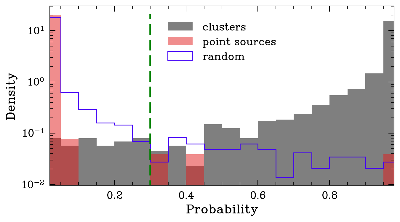
Figure 2: Distribution of probabilities predicted by our model for the test dataset: galaxy clusters are shown in grey, points sources are in red, and random fields are shown with purple curve. Each histogram is normalised by the total amount of objects of a given type. The green vertical line marks the probability threshold below which most of objects are actually non-clusters. We use this threshold in Section 4 to distinguish between non-clusters and cluster candidates.

3.1.4 Segmentation map

We apply our classifier to each pixel of ACT+Planck intensity maps and obtain a segmentation map. Each pixel in the segmentation map denotes a probability of a presence of the SZ signal in the direction of pixel centre.

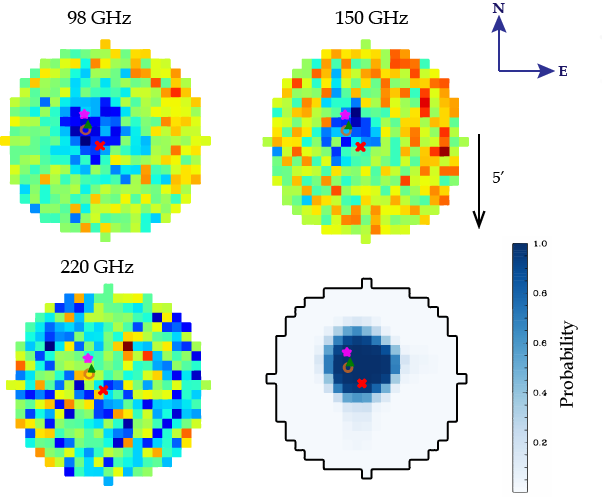
Figure 3: An example of a cluster detection in the direction of SZ_G098.31-41.19 (marked as the red cross) from the SZcat catalogue. 5-arcmin fragments of the ACT+Planck maps at different frequencies are shown in the upper row and in the bottom left panel. The pixel size is 0.5 arcmin. The probability map is presented at the bottom right corner. For comparison, we also show positions of clusters from PSZ2 (magenta star) and ACT DR5 (brown circle) catalogues which are within the cross-match radius, i.e. 5 arcmin circle. The pixel with maximum probability is marked as a green triangle.

An example of a patch of the segmentation map containing a massive galaxy cluster is shown in Fig. 3. We choose the direction of SZ_G098.31-41.19 (marked as the red cross) from the SZcat catalogue. The top row and the bottom left panel show three fragments of the ACT+Planck input maps at 98 GHz, 150 GHz, and 220 GHz. The probability map for this area is shown at the bottom right. It contains only one connected group within a chosen window, and this group can be associated with the galaxy cluster PSZ2 G098.30-41.15 from the PSZ2 catalogue (marked with a magenta star) and ACT-CL J2334.3+1759 from ACT DR5 (its centre is shown with a brown circle). It’s a massive cluster with $M_{500}\sim(7-8)10^{14}$ $M_{\odot}$ (Hilton, M. et al., 2021) located at $z=0.436$.

3.2 Detection model

Since galaxy clusters are extended objects, in the segmentation map we look for connected groups of pixels with probabilities above a certain threshold. To do so, we use the scikit-image (van der Walt et al., 2014) library developed for scientific image analysis in Python. We analyse manually a sample of probability maps for known clusters (i.e. patches of the segmentation map which contain galaxy clusters) and random fields on the sky (with no clusters) and derived the optimal value of the threshold segmentation $p_{seg}=0.3$ (see Fig. 2). For comparison, Bonjean (2020) used a threshold $p_{seg}=0.1$ to select sources in the SZ signal segmentation map created from Planck HFI imaging data.

Additionally, we remove the complex Galactic plane from consideration and keep only objects with the galactic latitude $|b|>15^{\circ}$. The resulting catalogue contains more than $1$ million potential SZ sources candidates with $p>0.3$ in the ACT footprint.

4 The ComPACT catalogue

Here, we aim to make a clean catalogue of cluster candidates using the SZcat catalogue (Meshcheryakov et al., 2022) as a basis. In the ACT field, the total number of SZcat sources is $14,850$.

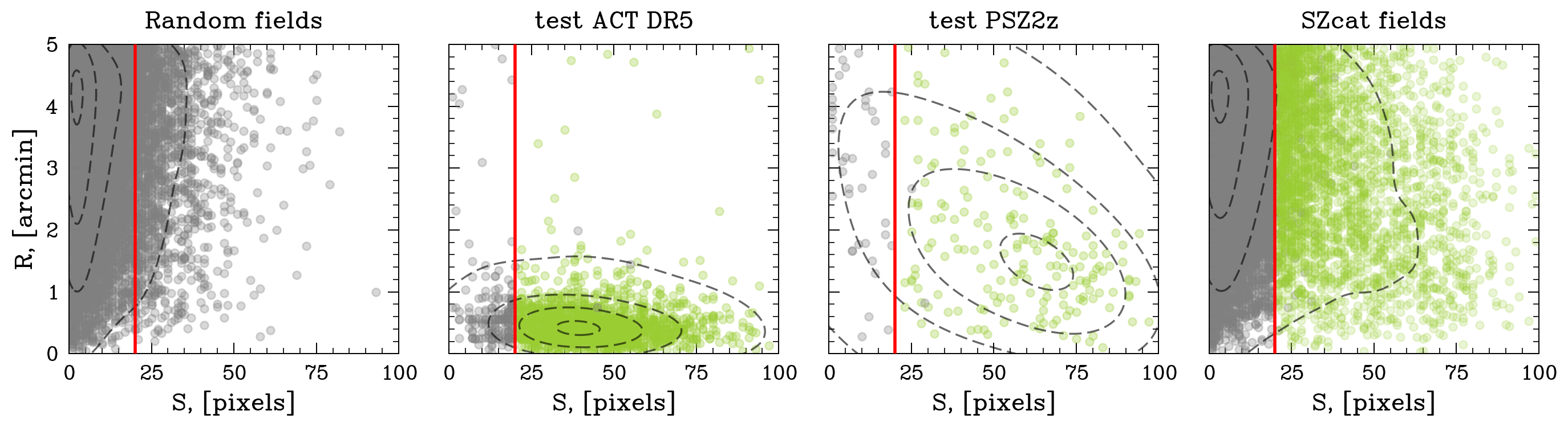
Figure 4: Distribution of connected groups of pixels according to their distance $R$ from the input direction and their area $S$. The left panel shows results for random directions that are unlikely to contain galaxy clusters. Density contours are shown as black dashed curves. Two central panels illustrate detected groups of pixels which corresponding to clusters from the ACT DR5 test subsample and spectroscopically confirmed clusters from PSZ2. The right panel shows the distribution of detected groups of pixels for SZcat directions. The latter plot combines characteristics of random fields and PSZ2 clusters since SZcat contains a quite number of false detections. Vertical red lines mark a threshold in area: we assume that all detected groups of pixels with $S<20$ are non-clusters. In green, we show groups that satisfy our criteria for clusters: $S>20$ and $p_{max}>0.8$

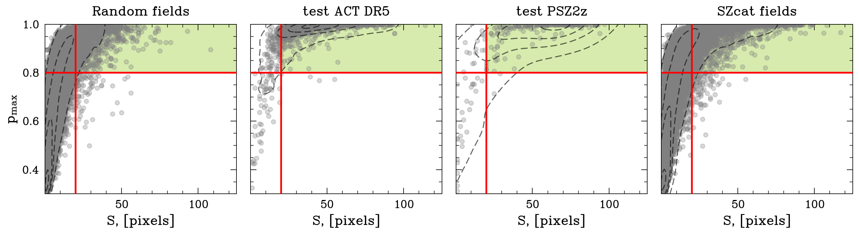
Figure 5: Group area $S$ — maximum probability within a group $p_{max}$ distributions. From left to right: random fields (in the ACT footprint), groups associated with optically confirmed galaxy clusters from the test ACT DR5 data set and from PSZ2z (in the ACT footprint), and SZcat directions (in the ACT footprint). Red lines indicates thresholds. With green colour we show a region where detected groups of pixels are classified as clusters: $S>20$ and $p_{max}>0.8$. We see that with this simple criterion in random fields almost all detected sources are classified as non-clusters, with only $\sim 10$% of groups falling into a ’cluster region’. For ACT DR5 and PSZ2 optically confirmed clusters we correctly classify $\sim 80$ % of clusters

For each direction from the SZcat catalogue we consider all detected connected groups of pixels in a window with $R_{match}=5$ arcmin. For each connected group we calculate (i) the group area $S$ (the total number of pixels in a given connected group), (ii) the maximum probability $p_{max}$ in a connected group, and (iii) the distance $R$ from the group centre (the pixel with $p_{max}$) to the input direction. We analyse different samples to form a criterion for distinguishing clusters from non-clusters among the connected groups (Figures 4 and 5). We come up with the following rule: a connected group is assigned to a cluster if its area $S>20$ pixels and its $p_{max}$ exceeds 0.8. As our tests show, with this criterion we reach a certain trade off between a purity and a completeness of the obtained catalogue of cluster candidates.

Let us now illustrate how a distribution of detected sources looks like on the $R$ – $S$ and $p_{max}$–$S$ planes for random directions on the sky (see the left panels of Fig. 4 and Fig. 5). Random fields are unlikely to contain galaxy clusters. We see that non-clusters tend to have low areas, lower values of $p_{max}$ when compared to clusters, and are offset from the input direction. In central panels of Fig. 4 and Fig. 5 we show distributions of clusters detected by our model along the input directions from the ACT DR5 test subsample (see Section 2) and from PSZ2z (the PSZ2 subsample of clusters with spectroscopic redshifts). All those objects are optically confirmed clusters. We see that real clusters tend to have large areas and large values of $p_{max}$. For ACT DR5 sources, $R$ is low ($\sim$ 1 arcmin for majority of clusters) since ACT has a good spatial resolution. For PSZ2z, clusters are more widely distributed in the $R$–$S$ plane because of poorer Planck resolution (compared to ACT). Right panels of Fig. 4 and Fig. 5 present distributions of connected groups of pixels detected by our model in the 5 arcmin window along the SZcat directions. Red lines in Figures 4 and 5 show thresholds in area $S=20$ and in maximum probability in a group $p_{max}=0.8$, which we use to distinguish clusters from non-clusters. We see that a low area - low $p_{max}$ region is densely populated. Most likely, these objects are non-clusters. At the same time, we detect a large number of sources with high area and high values of $p_{max}$ which are likely to be genuine clusters.

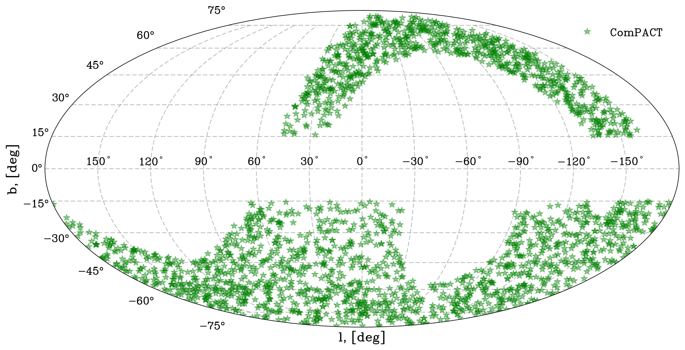
Figure 6: Distribution of ComPACT objects on the sky (in galactic coordinates)

In Fig. 6 we show a distribution of ComPACT clusters on the sky (in galactic coordinates).

4.1 Purity and completeness of the ComPACT catalogue

The key characteristics of a cluster catalogue are its purity and completeness metrics.

We estimate the ComPACT completeness with respect to PSZ2z (the subsample of PSZ2 objects with optical identification and cluster spectroscopic redshift measurements) and ACT DR5 cluster catalogues. We associate clusters from PSZ2z or ACT samples in the test area with the nearest object from our full catalogue of SZ candidates (see Section 3.2). All cluster associations are shown in the central panels of Figures 4 and 5. Then, we estimate the ComPACT catalogue completeness as

$$C=N^{\star}_{cl}/N_{cl}~{},$$ (3)

where $N^{\star}_{cl}$ is the number of clusters with $p_{max}>0.8$ and $S>20$ (green circles in the central panels of Fig. 4) and $N_{cl}$ is the total number of clusters in the considered sample. For the ACT DR5 and PSZ2z cluster samples, we obtain $C_{ACT}\approx 0.88$ and $C_{PSZ2z}\approx 0.79$. In both cases, $\sim 7\%$ of true clusters are not assigned to clusters by our (detection) model due to their low area, i.e. these objects have $S<20$. The decrease in the completeness of Planck clusters detection in ComPACT seems to be due to: (i) the way of combining ACT and Planck data in the joint intensity maps (Naess et al., 2020) and (ii) the wrong association between connected group and SZcat for some ComPACT clusters.

We define the purity of the ComPACT catalogue as:

$$Purity=1-\cfrac{N_{F}}{N_{ComPACT}}~{},$$ (4)

where $N_{F}$ and $N_{ComPACT}$ are the number of false detections and the total number of cluster candidates in the ComPACT catalogue, respectively. The number of false detections can be estimated as

$$N_{F}\lesssim{}(1-P)\cdot{}\hat{N}_{field}\cdot\bigg{(}\cfrac{N_{SZcat}}{N_{field}}\bigg{)}~{},$$ (5)

where $P=0.8$ is our threshold in the maximum probability ($p_{max}$), $\hat{N}_{field}$ and $N_{field}$ are the number of detections (connected groups of pixels) having $p_{max}>0.8$, $S>20$, and the total number of objects in the random fields sample, respectively; $N_{SZcat}$ is the total number of detections in the SZcat sample.

The idea behind formula (5) is simple. The subsample of detections in random fields with $p_{max}>0.8$ and $S>20$ contains more than $P\times 100\%=80\%$ of galaxy clusters. Thus, the number of false detections in this subsample can be estimated as $<(1-P)\cdot{}\hat{N}_{field}$. Then, we need to rescale the obtained estimate to the total amount of detections $N_{SZcat}$ in the fields of SZcat sources. It is worth noting, that equality (in terms of expected value) in the formula (5) can be achieved only if the SZcat objects are located in the random sky directions (in random fields) and all SZ detections have $p_{max}=0.8$.

Based on the expressions (4) and (5) one can obtain:

$$Purity\gtrsim 1-(1-P)\cdot\bigg{(}\cfrac{\hat{N}_{field}}{N_{field}}\bigg{)}\cdot\bigg{(}\cfrac{N_{SZcat}}{N_{ComPACT}}\bigg{)}~{}.$$ (6)

Substituting the corresponding values of $P$, $\hat{N}_{field}$, $N_{field}$, $N_{SZcat}$, $N_{ComPACT}$ into the formula (6) gives us the estimate of the ComPACT purity $\gtrsim{}0.88$.

Cluster catalogue	Number of objects	Sky fraction	Instrument	Ref
SZcat	14,850	0.88	Planck	Meshcheryakov et al. (2022)
PSZ2	1,653	0.84	Planck	Planck Collaboration (2016)
ACT DR5	4,195	0.32	ACT	Hilton, M. et al. (2021)
SPT-SZ	677	0.061	SPT	Bocquet et al. (2019)
ComPRASS	2,323	0.81	Planck, ROSAT	Tarrío, P. et al. (2019)
PSZSPT	419	0.061	SPT, Planck	Melin, J.-B. et al. (2021)
MCXC	1,743	0.38	ROSAT, EXOSAT	Piffaretti et al. (2011)
4XMM-DR12	88,169	0.028	XMM-Newton	Webb et al. (2020)
ComPACT	2,934	0.37	ACT+Planck	this paper

Table 2: External galaxy cluster samples in comparison with new ComPACT cluster catalogue presented in this paper.

4.2 Cross-correlation of ComPACT with external cluster catalogues

Figure 7: Number of cross-matches of ComPACT cluster candidates with other catalogues. The left panel shows all candidates, the right panel shows only ComPACT candidates that have no matches with ACT DR5 or PSZ2 catalogues. In each panel, the first line shows the total number of ComPACT objects in a considered sample/subsample. In blue, the expected amount of genuine clusters (number of candidates multiplied by purity) is shown. The second line illustrates the total number of matches across explored catalogues. The remaining lines represent the number of matches with a given catalogue.

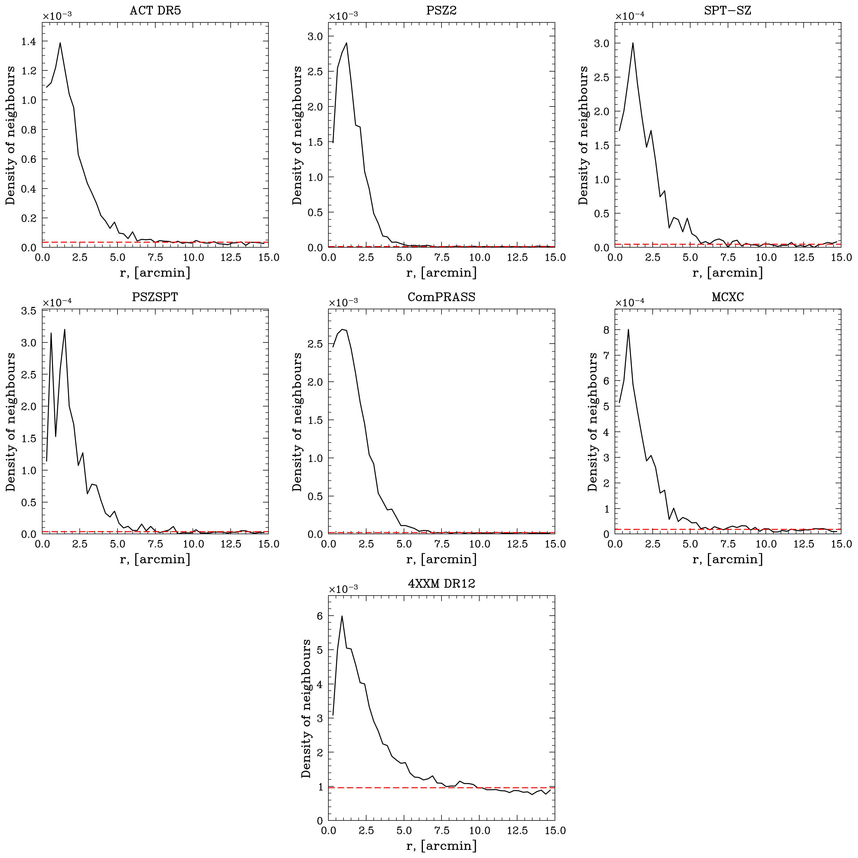
Figure 10: Average number density of clusters (from different catalogues) as a function of radius to SZcat sources. The dashed horizontal line shows the mean density.

We cross-correlate the derived ComPACT sample with the following X-ray and SZ external cluster catalogues: MCXC, 4XMM DR12, ACT DR5, PSZ2, SPT SZ, ComPRASS, and PSZSPT. The cross-match radius is set to 5 arcmin. This choice is motivated by the analysis of average number density radial profiles (for different cluster catalogues) in the neighbourhood of ComPACT objects (see Figure 10). Table 2 gives the summary information about external cluster catalogues in comparison with ComPACT. From ACT DR5, we identify 1,033 matches, cross-correlation with the PSZ2 catalogue gives 482 clusters.

Also, we find ComPACT objects matches in cluster catalogues other than ACT DR5 and PSZ2. We identify 2 clusters in SPT-SZ, 3 clusters in PSZSPT, 67 objects in ComPRASS, 47 objects as extended X-ray sources in 4XMM DR12, 16 objects in MCXC. All ComPACT objects identified as X-ray galaxy clusters with luminosity (in the energy band 0.5-2 keV) exceeding $7.5\cdot 10^{44}\>erg/s$ have $p_{max}\sim 1$.

In Fig. 7 (left panel), we show numbers of ComPACT clusters associated with different external cluster catalogues. ComPACT contains $2,934$ cluster candidates, among which $\gtrsim{}2,581$ objects are expected to be real galaxy clusters (see §4.1 for ComPACT catalogue purity estimate). A total number of 1,259 objects are associated with sources from external cluster catalogues, among which 1,146 clusters are found in Planck and/or ACT cluster catalogues. $1,788$ ComPACT objects are new with respect to the existing ACT DR5 or PSZ2 cluster samples, among them we expect $\gtrsim 1,436$ real clusters.

In Fig. 7 (right panel), we show numbers of ComPACT clusters not found in PSZ2/ACT cluster catalogues and associated with objects from other cluster samples. One can see, that among expected $\gtrsim 1,436$ real clusters (not found in PSZ2/ACT DR5), 113 objects are found in MCXC, 4XMM DR12, SPT-SZ, ComPRASS, PSZSPT catalogues. Thus, we expect $\gtrsim 1,366$ totally new clusters in ComPACT.

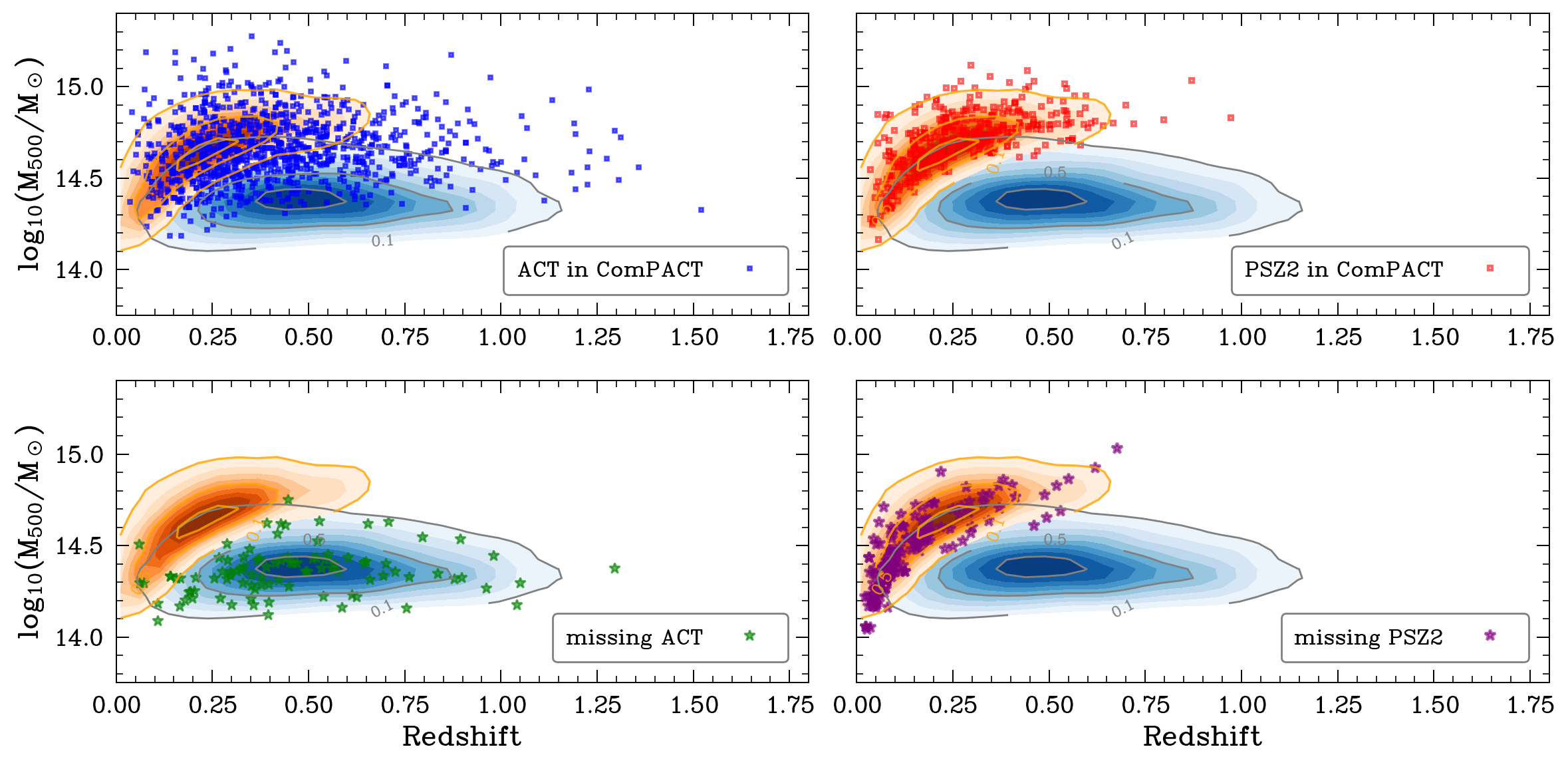
Figure 8: ComPACT cluster candidates cross-matched with ACT DR5 (1,033 objects; blue dots in the upper left panel) and PSZ2 (418 objects; orange dots in the upper right panel). On the bottom panel we present clusters from ACT DR5 (green stars) and PSZ2 (purple stars) that have SZcat candidates within a 5 arcmin radius, but are not presented in ComPACT. Blue contours show density of SZ sources in ACT DR5 on the mass-redshift plane, while orange contours represent density of PSZ2 sources. From comparing ComPACT candidates matched with ACT DR5 and density contours of ACT DR5 sources, it appears that we miss low-mass clusters especially at intermediate and high redshifts. It might be due to our cluster detection criteria and because ComPACT is based on SZcat, which in turn is constructed from Planck maps.

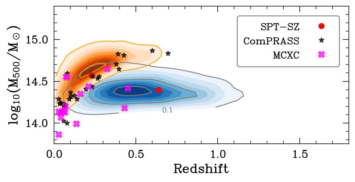
Figure 9: Mass-redshift dependence for ComPACT cluster candidates which do not have matches with ACT DR5 or PSZ2 but do have with MCXC (magenta crosses), ComPRASS (black stars), and SPT-SZ (red circles). The orange density contours show density of PSZ2 sources, the blue one - ACT DR5 clusters.

In Figure 9, we illustrate the mass-redshift dependence for clusters in ACT DR5 and PSZ2z catalogues. The blue and orange contours represent the distributions of the full ACT DR5 and PSZ2z catalogues, respectively. For ACT DR5, we ‘recover’ 1,033 clusters (shown as blue squares in the upper left panel), and 95 ACT clusters are missing in ComPACT (shown as green stars in the bottom left panel). We miss low-mass cluster candidates at intermediate and high redshifts due to (i) detection limitations of the SZcat catalogue, and (ii) our area criterion (see the second panel of Figure 4).

The mass-redshift distribution for PSZ2 matches in ComPACT is plotted as red squares in the upper right panel of Fig. 9. PSZ2z clusters that are not present in ComPACT are shown as purple stars (291 objects) in the bottom right panel of Fig. 9.

Let us now discuss cluster candidates that do not have any matches in ACT DR5 or PSZ2 catalogues. In Figure 9, we plot matches (with available in the literature masses and redshifts) with SPT-SZ (red dots), ComPRASS (black stars), and MCXC (magenta crosses). Most of them lie at $z<0.8$. Compared to the ACT DR5 catalogue, ComPACT is more complete at lower redshifts. We expect to find objects with low mass at low redshifts and clusters on the border of PSZ2 density distribution.

5 Conclusions

Galaxy clusters are the most massive gravitationally bound systems consisting of dark matter, hot baryonic gas and stars. They play an important role in observational cosmology and galaxy evolution studies. We have created a deep learning model for segmentation of SZ signal on ACT+Planck intensity maps (Naess et al., 2020) and present here a new galaxy cluster catalogue in the ACT footprint.

In order to increase the purity of the cluster catalogue, we limit ourselves to publishing here only a part of the full sample with the most probable galaxy clusters lying in the directions to the candidates of the extended Planck cluster catalogue (SZcat, Meshcheryakov et al. (2022)). The ComPACT catalogue contains 2,934 galaxy clusters with $Purity\gtrsim 88$%.

Note that $\gtrsim 1,436$ SZ clusters in the presented ComPACT catalogue are new with respect to the existing ACT DR5 and PSZ2 cluster samples. In the future work we plan to identify these objects in the optical surveys, estimate their total masses and redshifts.

Data availability

The ComPACT cluster catalogue is publicly available: https://github.com/astromining/ComPACT

Appendix A Description of the ComPACT catalogue

Table 3: Sample of 5 rows from ComPACT

Name RA DEC S pmax SZcat ACT PSZ2 ComPACT_G68.671-52.228 -16.983333 -2.408333 27 0.987531 SZ_G068.57-52.25 - - ComPACT_G64.577-58.808 -13.616667 -8.525000 27 0.840159 SZ_G064.59-58.75 - - ComPACT_G7.579-33.928 -53.083333 -34.800000 59 0.998711 SZ_G007.56-33.94 ACT-CL J2027.6-3447 PSZ2 G007.57-33.90 ComPACT_G32.32337.037 -111.216667 15.491667 77 0.999866 SZ_G032.32+37.03 ACT-CL J1635.1+1529 - ComPACT_G208.385-28.424 75.408333 -8.916667 73 0.996167 SZ_G208.45-28.38 - -

The ComPACT catalogue contains 2,934 galaxy cluster candidates ($Purity\gtrsim 88$%). Below we describe columns of the catalogue.

Name :

ID of a ComPACT object.

RA :

Object right ascension (in degrees, J2000 epoch). Centre of object corresponds to pixel with highest SZ signal probability in the source area.

DEC :

Object declination (in degrees, J2000 epoch).

S :

Object area (pixels with $p>0.3$) on the SZ signal segmentation map (in pixels)

pmax :

SZ signal probability (in the object centre).

SZcat :

SZcat object name.

ACT :

ACT DR5 cluster name.

PSZ2 :

PSZ2 cluster name.

Appendix B Description of external cluster catalogues

Below is a description of the catalogues used, which were not described in the main part of the article

B.1 PSZ2

The Planck Sunyaev-Zeldovich 2 (PSZ2, Planck Collaboration (2016)) cluster catalogue contains clusters with a high level of significance ($S/N>4.5$). The total number of objects is 1,653. The PSZ2 catalogue includes galaxy clusters with redshifts up to z = 0.8. The multi-frequency matched filter algorithm (MMF1 Herranz et al. (2002), MMF3 Melin, J.-B. et al. (2006)) and PowellSnakes Carvalho et al. (2012) were used to find SZ objects. In the ACT footprint, there are 867 clusters. Among those, 623 clusters have also measurements of spectroscopic redshifts. We call this subsample of the Planck catalogue as PSZ2z.

B.2 SPT-SZ

The South Pole Telescope (SPT) observes the southern sky at 95, 150, and 220 GHz with an angular resolution of 1-1.6 minutes (Carlstrom, J. E. et al., 2011). We use the SPT-SZ cluster catalogue (Bocquet et al., 2019). It contains 677 SZ objects, 516 of which have been confirmed as clusters using optical and near-infrared observations. 597 SPT-SZ clusters are in the ACT footprint.

B.3 PSZSPT

The PSZSPT (Melin, J.-B. et al., 2021) catalogue combines data from the Planck Space Telescope and the SPT ground-based telescope. The catalogue was obtained by using multi-frequency matched filtering and contains 419 clusters (with $S/N>5$), 373 of which lie in the ACT footprint.

B.4 ComPRASS

Planck microwave data and RASS (ROSAT All-Sky Survey, Tarrío, P. et al. (2019)) X-ray data were combined to create the catalogue. The catalogue contains 2,323 objects (including confirmed clusters and cluster candidates), with 1,110 objects are in the ACT footprint.

B.5 MCXC

The MCXC meta catalogue (Piffaretti et al., 2011) contains 1,868 X-ray clusters detected in ROSAT and EXOSAT data (by various groups) with optical identifications. 867 X-ray clusters are in the ACT footprint.

B.6 XMM-Newton clusters

4XMM-DR12 catalogue (Webb et al., 2020) contains X-ray sources from 12,712 XMM-Newton EPIC observations. Among them 88,169 objects are marked as extended (Extent>0). 35,756 X-ray clusters are in the ACT footprint.

References

- Allen et al. (2011) Allen S. W., Evrard A. E., Mantz A. B., 2011, Annual Review of Astronomy and Astrophysics, 49, 409
- Bertin & Arnouts (1996) Bertin E., Arnouts S., 1996, A&AS, 117, 393
- Bleem et al. (2015) Bleem L. E., et al., 2015, The Astrophysical Journal Supplement Series, 216, 27
- Bocquet et al. (2015) Bocquet S., et al., 2015, ApJ, 799, 214
- Bocquet et al. (2019) Bocquet S., et al., 2019, ApJ, 878, 55
- Bonjean (2020) Bonjean V., 2020, Astronomy & Astrophysics, 634, A81
- Burenin (2013) Burenin R. A., 2013, Astronomy Letters, 39, 357
- Burenin (2017) Burenin R. A., 2017, Astronomy Letters, 43, 507
- Burenin (2018) Burenin R. A., 2018, Astronomy Letters, 44, 653
- Burenin & Vikhlinin (2012) Burenin R. A., Vikhlinin A. A., 2012, Astronomy Letters, 38, 347
- Burke et al. (2019) Burke C. J., Aleo P. D., Chen Y.-C., Liu X., Peterson J. R., Sembroski G. H., Lin J. Y.-Y., 2019, MNRAS, 490, 3952
- Carlstrom, J. E. et al. (2011) Carlstrom, J. E. et al., 2011, Publications of the Astronomical Society of the Pacific, 123, 568
- Carvalho et al. (2012) Carvalho P., Rocha G., Hobson M. P., Lasenby A., 2012, Monthly Notices of the Royal Astronomical Society, 427, 1384
- Datta et al. (2019) Datta R., et al., 2019, MNRAS, 486, 5239
- Dubey et al. (2021) Dubey S. R., Singh S. K., Chaudhuri B. B., 2021, arXiv e-prints, p. arXiv:2109.14545
- Gralla et al. (2020) Gralla M. B., et al., 2020, The Astrophysical Journal, 893, 104
- Harris et al. (2020) Harris et al., 2020, Nature, 585, 357
- Hartley et al. (2023) Hartley P., et al., 2023, MNRAS, 523, 1967
- Herranz et al. (2002) Herranz D., Sanz J. L., Hobson M. P., Barreiro R. B., Diego J. M., Martínez-González E., Lasenby A. N., 2002, Monthly Notices of the Royal Astronomical Society, 336, 1057
- Hilton, M. et al. (2021) Hilton, M. et al., 2021, The Astrophysical Journal Supplement Series, 253, 3
- Hinton et al. (2012) Hinton G. E., Srivastava N., Krizhevsky A., Sutskever I., Salakhutdinov R. R., 2012, Improving neural networks by preventing co-adaptation of feature detectors (arXiv:1207.0580)
- Hunter (2007) Hunter J. D., 2007, Computing in Science & Engineering, 9, 90
- Ioffe & Szegedy (2015) Ioffe S., Szegedy C., 2015, Batch Normalization: Accelerating Deep Network Training by Reducing Internal Covariate Shift, doi:10.48550/ARXIV.1502.03167, https://arxiv.org/abs/1502.03167
- Kingma & Ba (2017) Kingma D. P., Ba J., 2017, Adam: A Method for Stochastic Optimization (arXiv:1412.6980)
- Kravtsov & Borgani (2012) Kravtsov A. V., Borgani S., 2012, ARA&A, 50, 353
- Kravtsov et al. (2006) Kravtsov A. V., Vikhlinin A., Nagai D., 2006, ApJ, 650, 128
- Lin et al. (2021) Lin Z., Huang N., Avestruz C., Wu W. L. K., Trivedi S., Caldeira J., Nord B., 2021, MNRAS, 507, 4149
- Maas, A.L. & Ng, A.Y. (2013) Maas, A.L. H., Ng, A.Y. 2013. https://ai.stanford.edu/~amaas/papers/relu_hybrid_icml2013_final.pdf
- Mantz et al. (2015) Mantz A. B., et al., 2015, MNRAS, 446, 2205
- Melin, J.-B. et al. (2006) Melin, J.-B. Bartlett, J. G. Delabrouille, J. 2006, A&A, 459, 341
- Melin, J.-B. et al. (2021) Melin, J.-B. Bartlett, J. G. Tarrío, P. Pratt, G. W. 2021, A&A, 647, A106
- Meshcheryakov et al. (2022) Meshcheryakov A. V., Nemeshaeva A., Burenin R. A., Gilfanov M. R., Sunyaev R. A., 2022, Astronomy Letters, 48, 479
- Naess et al. (2020) Naess S., et al., 2020, Journal of Cosmology and Astroparticle Physics, 2020, 046
- Oliphant (2006) Oliphant T., 2006, Guide to NumPy
- Paszke et al. (2019) Paszke A., et al., 2019, in Advances in Neural Information Processing Systems. Curran Associates, Inc., https://proceedings.neurips.cc/paper_files/paper/2019/file/bdbca288fee7f92f2bfa9f7012727740-Paper.pdf
- Piffaretti et al. (2011) Piffaretti R., Arnaud M., Pratt G. W., Pointecouteau E., Melin J. B., 2011, A&A, 534, A109
- Planck Collaboration (2016) Planck Collaboration 2016, A&A, 586, A139
- Planck Collaboration (2014) Planck Collaboration 2014, A&A, 571, A21
- Planck Collaboration (2016) Planck Collaboration 2016, A&A, 594, A27
- Planck Collaboration et al. (2013) Planck Collaboration et al., 2013, A&A, 550, A129
- Planck Collaboration et al. (2016a) Planck Collaboration et al., 2016a, A&A, 594, A13
- Planck Collaboration et al. (2016b) Planck Collaboration et al., 2016b, A&A, 594, A24
- Pratt et al. (2019) Pratt G. W., Arnaud M., Biviano A., Eckert D., Ettori S., Nagai D., Okabe N., Reiprich T. H., 2019, Space Science Reviews, 215
- Raghunathan et al. (2022) Raghunathan S., et al., 2022, ApJ, 926, 172
- Sarazin (1988) Sarazin C. L., 1988, X-ray emission from clusters of galaxies
- Simonyan & Zisserman (2015) Simonyan K., Zisserman A., 2015, Very Deep Convolutional Networks for Large-Scale Image Recognition (arXiv:1409.1556)
- Sunyaev & Zeldovich (1970) Sunyaev R. A., Zeldovich Y. B., 1970, Ap&SS, 7, 3
- Sunyaev & Zeldovich (1972) Sunyaev R. A., Zeldovich Y. B., 1972, Comments on Astrophysics and Space Physics, 4, 173
- Tarrío, P. et al. (2019) Tarrío, P. Melin, J.-B. Arnaud, M. 2019, A&A, 626, A7
- Verkhodanov et al. (2021) Verkhodanov O. V., Topchieva A. P., Oronovskaya A. D., Bazrov S. A., Shorin D. A., 2021, Astrophysical Bulletin, 76, 123
- Vikhlinin et al. (2009) Vikhlinin A., et al., 2009, ApJ, 692, 1060
- Webb et al. (2020) Webb N. A., et al., 2020, A&A, 641, A136
- Wes McKinney (2010) Wes McKinney 2010, in Stéfan van der Walt Jarrod Millman eds, Proceedings of the 9th Python in Science Conference. pp 56 – 61, doi:10.25080/Majora-92bf1922-00a
- Williamson et al. (2011) Williamson R., et al., 2011, The Astrophysical Journal, 738, 139
- pandas development team (2023) pandas development team T., 2023, pandas-dev/pandas: Pandas, doi:10.5281/zenodo.7794821, https://doi.org/10.5281/zenodo.7794821
- van der Walt et al. (2011) van der Walt S., Colbert S. C., Varoquaux G., 2011, Computing in Science & Engineering, 13, 22
- van der Walt et al. (2014) van der Walt S., et al., 2014, PeerJ, 2, e453