Optical fibres with memory effects and their quantum communication capacities

The development of quantum repeaters poses significant challenges in terms of cost and maintenance, prompting the exploration of alternative approaches for achieving long-distance quantum communication. In the absence of quantum repeaters and under the memoryless (iid) approximation, it has been established that some fundamental quantum communication tasks are impossible if the transmissivity of an optical fibre falls below a known critical value, resulting in a severe constraint on the achievable distance for quantum communication. However, if the memoryless assumption does not hold — e.g. when input signals are separated by a sufficiently short time interval — the validity of this limitation is put into question. In this paper we introduce a model of optical fibre that can describe memory effects for long transmission lines. We then solve its quantum capacity, two-way quantum capacity, and secret-key capacity exactly. By doing so, we show that — due to the memory cross-talk between the transmitted signals — reliable quantum communication is attainable even for highly noisy regimes where it was previously considered impossible. As part of our solution, we find the critical time interval between subsequent signals below which quantum communication, two-way entanglement distribution, and quantum key distribution become achievable.

Quantum information NC , and in particular quantum communication, will likely play a pivotal role in our future technology. The potential applications of a global quantum internet quantum_internet_Wehner ; Pirandola20 include secure communication bennett1984quantum , efficient entanglement and qubits distribution, enhanced quantum sensing capabilities Sidhu , distributed and blind quantum computing Distributed_QC ; secure_access_qinternet , as well as groundbreaking experiments in fundamental physics Sidhu . These applications heavily rely on establishing long-distance quantum communication across optical fibres or free-space links. However, the vulnerability of optical signals to noise poses a significant obstacle to achieve this goal. To overcome this challenge, one possible known solution is to exploit quantum repeaters repeaters ; Munro2015 along the communication line. Nonetheless, current implementations of quantum repeaters remain in the realm of proof-of-principle experiments. In addition, quantum repeaters will likely impose substantial demands on technology resources, making them potentially expensive to implement. Consequently, a pressing problem is to develop quantum communication protocols that can operate without — or with a modest number of — quantum repeaters. Recently, in Die-Hard-2-PRL ; Die-Hard-2-PRA it has been proposed a theoretical proof-of-principle solution to the problem of establishing quantum communication over long distance without relying on quantum repeaters. The crux of such a solution is to take advantage of memory effects memory-review ; Dynamical-Model in optical fibres.

Memory effects arise when signals are fed into the optical fibre separated by a sufficiently short time interval memory-review ; Dynamical-Model ; Banaszek-Memory ; Ball-Memory . In this scenario, the noise within the fibre is influenced by prior input signals, exhibiting a form of "memory." Consequently, the commonly assumed memoryless (iid) paradigm, which posits that noise acts uniformly and independently on each signal, becomes invalid. The exploration of memory effects in optical fibres has been extensively addressed in Memory1 ; Memory2 ; Memory3 ; Die-Hard-2-PRA ; Die-Hard-2-PRL . These studies primarily focus on modelling the interaction between two signals through a single localised interaction. While they capture fundamental aspects of the problem, especially in the context of "short" communication lines or setups with signal cross-talk confined in a specific spatial region, a more comprehensive analysis reveals limitations when extending these findings to practical configurations. Specifically, in scenarios involving "long" communication lines where consecutive signals continually interact throughout the entire length of the fibre, the existing analyses become inadequate, hindering the incorporation of two essential requirements vital for the theory’s conceptual self-consistency:

• Property 1: It is imperative that no information can be transmitted across the fibre if the transmissivity associated with a single signal is precisely zero;

• Property 2: The model must remain consistent when optical fibres are composed. In other words, the combination of the model associated with a fibre of length $L_{1}$ and the model linked to a fibre of length $L_{2}$ should yield the model associated with a fibre of length $L_{1}+L_{2}$.

Aim of the present paper is to overcome the limitations of Memory1 ; Memory2 ; Memory3 ; Die-Hard-2-PRA ; Die-Hard-2-PRL by developing a new model of optical fibres with memory effects that accurately encapsulates the essential attributes of extended optical fibres, such as those outlined in Properties 1 and 2 above. We shall call such model "Delocalised Interaction Model", or DIM in brief, and employ it to determine the ultimate quantum communication capabilities attainable through the strategic utilisation of memory effects in these systems. In particular, we will find the precise range of parameters that allow for the successful transmission of qubits, entanglement, or secret keys. Our main result is the calculation of the exact value of the quantum capacity $Q$, the two-way quantum capacity $Q_{2}$, and the secret-key capacity $K$ MARK ; Sumeet_book of the optical fibre in the absence of thermal noise. Additionally, our investigation will encompass an examination of the existence of the phenomenon known as the "die-hard quantum communication" effect die-hard ; Die-Hard-2-PRL ; Die-Hard-2-PRA . This effect, potentially enabling communication across optical fibres with arbitrarily low transmissivity, will be scrutinised to confirm its presence in our model, ensuring it is not merely an artifact of the localised signal cross-talking assumption made in die-hard ; Die-Hard-2-PRL ; Die-Hard-2-PRA . Specifically we shall see that for any arbitrarily low non-zero value of the single-signal transmissivity $\lambda\in(0,1]$ of the fibre and for any arbitrarily large value of its associated thermal noise $\nu\geq 0$, there exists a non-zero time interval separating successive signals below which $Q$, $Q_{2}$, and $K$ all become strictly positive. In particular, we show that memory effects enable qubit distribution ($Q>0$) even when $\lambda\in(0,\frac{1}{2}]$, which is not achievable with the corresponding memoryless optical fibre. Additionally, using the sufficient condition for entanglement distribution reported in lower-bound , we show that memory effects enable two-way entanglement distribution ($Q_{2}>0$) and quantum key distribution ($K>0$) even when $\lambda\in(0,\frac{\nu}{\nu+1}]$, thus surpassing the performance of memoryless optical fibres.

Preliminaries

In the framework of quantum Shannon theory MARK ; Sumeet_book , the fundamental limitations of point-to-point quantum communication are determined by the capacities of quantum channels. The capacities quantify the maximum amount of information that can be reliably transmitted per channel use in the asymptotic limit of many uses. Different notions of capacities have been defined, based on the type of information to be transmitted, such as qubits or secret-key bits, and the additional resources permitted in the protocol design, such as classical feedback. In this paper, we investigate three distinct capacities: on the one hand the quantum capacity $Q$, which measures the efficiency in the transmission of qubits with no additional resources; on the other, the two-way quantum capacity $Q_{2}$ and the secret-key capacity $K$, which instead gauge the efficiency in the transmission of qubits and secret key, respectively, with the additional free resource of a public two-way classical communication channel between the sender (Alice) and the receiver (Bob) MARK ; Sumeet_book .

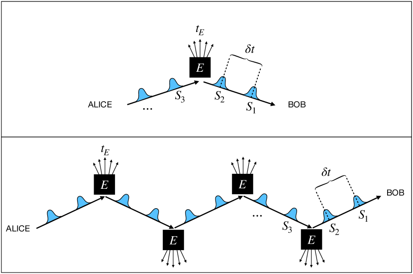
Figure 1: Pictorial representation of the mechanism which is responsible for the intra-signal interactions between a sequence of pulses $S_{1}$, $S_{2}$, $\cdots$ that travel along an optical fibre. In the LIM Memory1 ; Memory2 ; Memory3 such couplings occurs in a single location, through the mediation of a single common environment (upper panel). A more realistic description of the effect would instead allow for multiple cross-talks events distributed over the entire length of the fibre (bottom panel).

The signals transmitted along an optical fibre can be described in terms of an ordered array of localised e.m. pulses $S_{1}$, $S_{2}$, $\cdots$, $S_{n}$, of assigned mean frequency $\omega_{0}$ and bandwidth $\Delta\omega$ that, in the absence of dispersion, propagate rigidly through the fibre separated by a fixed delay time $\delta t$. In the quantum setting such modes are conventionally identified with a corresponding collection of independent annihilation operators $a_{1}$, $a_{2}$, $\cdots$, $a_{n}$ that fulfil canonical commutation rules Caves . The memoryless regime is reached when $\delta t$ is sufficiently large to prevent cross-talking among the transmitted signals: accordingly they will experience the same type of noise which, under very general conditions, is typically identified with a thermal attenuator channel $\mathcal{E}_{\lambda,\nu}$. This is a continuous-variable BUCCO single-mode quantum channel characterised by two parameters: $\lambda\in[0,1]$, which represents the transmissivity of the fibre (i.e. the ratio between the output energy and the input energy of the transmitted signal), and $\nu\in[0,\infty)$, which quantifies the thermal noise added by the environment (in the limit of zero temperature $\nu=0$, the transformation is conventionally referred to as the pure-loss channel). Mathematically, the action of $\mathcal{E}_{\lambda,\nu}$ on a generic input state $\rho$ of the $i$th signal can be expressed as a beam splitter mixing the latter with a dedicated local Bosonic bath $E_{i}$, initialised in the thermal state $\tau_{\nu}$ with mean photon number $\nu$. In formula, this can be written as

$$\mathcal{E}_{\lambda,\nu}(\rho) \coloneqq\operatorname{Tr}_{E_{i}}\left[U_{\lambda}\big{(}\rho\otimes\tau_{\nu}\big{)}{U_{\lambda}}^{\dagger}\right]\,,$$ (1)

where $a_{i}$ and $b_{i}$ are the annihilation operators of $S_{i}$ and $E_{i}$, $U_{\lambda}\coloneqq e^{\arccos(\sqrt{\lambda})(a_{i}^{\dagger}b_{i}-a_{i}\,b_{i}^{\dagger})}$ is the unitary describing the beam splitter interaction, and $\operatorname{Tr}_{E_{i}}$ represents the partial trace w.r.t. $E_{i}$. The capacities $Q$ holwer ; LossyECEAC1 ; LossyECEAC2 , $Q_{2}$ PLOB , and $K$ PLOB of the pure-loss channel $\mathcal{E}_{\lambda,0}$ have been determined exactly. In contrast, only bounds are known for the capacities $Q$ PLOB ; Rosati2018 ; Sharma2018 ; Noh2019 ; holwer ; Noh2020 ; fanizza2021estimating , $Q_{2}$ PLOB ; Pirandola2009 ; Ottaviani_new_lower ; lower-bound , and $K$ PLOB ; Pirandola2009 ; Ottaviani_new_lower ; lower-bound of the thermal attenuator $\mathcal{E}_{\lambda,\nu}$. In particular, it is known that the quantum capacity of the thermal attenuator $Q(\mathcal{E}_{\lambda,\nu})$ vanishes if the transmissivity of the fibre falls below the critical value of $\lambda\leq\frac{1}{2}$:

$$\lambda\leq\frac{1}{2}\Longrightarrow Q(\mathcal{E}_{\lambda,\nu})=0\,,$$ (2)

and, additionally, the equivalence "$\Longleftrightarrow$" holds for $\nu=0$. It is also known that the two-way quantum capacity $Q_{2}(\mathcal{E}_{\lambda,\nu})$ and the secret-key capacity $K(\mathcal{E}_{\lambda,\nu})$ of the thermal attenuator vanish if and only if the transmissivity falls below the critical value of $\lambda\leq\frac{\nu}{\nu+1}$ lower-bound :

$$\lambda\leq\frac{\nu}{\nu+1}\Longleftrightarrow Q_{2}(\mathcal{E}_{\lambda,\nu})=K(\mathcal{E}_{\lambda,\nu})=0\,.$$ (3)

Since typically the transmissivity of an optical fibre decreases exponentially with its length, under the memoryless assumption there are strong limitations on the distance at which it is possible to perform qubit distribution $(Q>0)$, two-way entanglement distribution $(Q_{2}>0)$, and quantum key distribution $(K>0)$ without relying on quantum repeaters. For instance, modern optical fibres typically exhibit signal attenuation rates of around $0.2\text{\,}\mathrm{dB}\text{/}\mathrm{km}$, with the best recorded value being $0.14\text{\,}\mathrm{dB}\text{/}\mathrm{km}$ Tamura2018 ; Li2020 , meaning that the quantum capacity vanishes if the fibre is longer than $15\text{\,}\mathrm{km}$ or at most $21\text{\,}\mathrm{km}$.

Early attempts to incorporate memory effects into optical fibres were made in Refs. Memory1 ; Memory2 ; Memory3 with a model which from now on we shall refer to as "Localised Interaction Model" (LIM). In these works, following the approach outlined in Dynamical-Model , intra-signal couplings are induced by an ordered sequence of collisional events in which each transmitted pulse interacts with a common reservoir $E$ (see upper panel of Fig. 1). The latter is characterised by a resetting mechanism that endeavors to restore it to its initial configuration over a thermalization time-scale $t_{E}$. Consequently, when the time delay $\delta t$ separating two successive input signals exceeds the thermalization time $t_{E}$, each pulse encounters the same environmental state, rendering the communication effectively memoryless. Conversely, when $\delta t$ is smaller than or comparable to $t_{E}$, after colliding with one of the signals, the reservoir $E$ does not have sufficient time to revert to $\tau_{\nu}$ and functions as a mediator for pulse interactions. As illustrated in Fig. 2(b), LIM emulates this intricate dynamics of the $n$ input signals via the $n$-mode quantum channel $\Phi_{\lambda,\mu,\nu}^{(1,n)}$, obtained by connecting the parallel optical lines which describe the noisy propagation of the modes associated with the annihilation operators $a_{1}$, $a_{2}$, $\cdots$, $a_{n}$ in the memoryless regime (panel (a) of Fig. 2), with a series of additional beam splitters of transmissivity $\mu$. This parameter serves as the "memory parameter" of the model, quantifying what is the fraction of the energy lost by the $i$th input signal that can potentially be absorbed by the subsequent ones by mixing it with the thermal contributions of the local environments $E_{i+1}$, $E_{i+2}$, $\cdots$, $E_{n}$. Ranging from $0$ (where $\Phi_{\lambda,0,\nu}^{(1,n)}$ reduces to $n$fold memoryless channels ${\mathcal{E}}_{\lambda,\nu}^{\otimes n}$) to $1$ (full memory), $\mu$ effectively encapsulates the interplay between the time interval $\delta t$ separating two consecutive input signals and the characteristic thermalization time $t_{E}$ (for instance, one plausible expression for $\mu$ might be defined as $\mu\coloneqq\exp(-\delta t/t_{E})$). Note also that similarly to the memoryless case, the LIM transformation $\Phi_{\lambda,\mu,\nu}^{(1,n)}$ is still characterised by an effective transmissivity parameter $\lambda$ which in this case represents the attenuation experienced when a single signal traverses the line in isolation, and by the thermal noise parameter $\nu$ which is responsible for defining the temperature of the local baths.

A crucial insight which emerges from Refs. Memory1 ; Memory2 ; Memory3 is that memory couplings can improve the communication efficiency of optical fibres, thus opening the door to the realisation of the "die-hard quantum communication" effect die-hard ; Die-Hard-2-PRL ; Die-Hard-2-PRA . For instance, in the zero-temperature ($\nu=0$) limit the value of $Q$ computed for LIM turns out to be an increasing function of $\mu$ for each assigned transmissivity value $\lambda$ (see also Appendix VI). Unfortunately, as outlined in the introduction, utilising LIM for investigating real-world scenarios is problematic, mainly because it fails to consider the possibility that the signals could experience multiple cross-talks over different locations of the optical fibre as depicted in the bottom panel of Fig. 1. The limitations of LIM become particularly evident when one observes that the associated mapping $\Phi_{\lambda,\mu,\nu}^{(1,n)}$ does not fulfil neither Property 1 nor Property 2, which should instead hold for long transmission lines. For instance, a close inspection of the interferometric representation of Fig. 2(b) reveals that, as long as $\mu>0$, even for $\lambda=0$ the channel $\Phi_{0,\mu,\nu}^{(1,n)}$ is still capable of transmitting signals from Alice to Bob (e.g. the photons of the first input mode $a_{1}$ will be received by Bob at the output of the mode $a_{2}$). The possibility of having multiple cross-talks will arguably prevent this possibility via destructive interferences that could in principle spoil the advantages pointed out in Memory1 ; Memory2 ; Memory3 ; die-hard ; Die-Hard-2-PRL ; Die-Hard-2-PRA . The primary objective of this paper is to shed light on this problem, introducing a new model for memory effects in optical fibres that is immune to the shortcomings of LIM.

Results

In this section we present an improved version of LIM which can be used to describe memory effects in optical fibres when the transmitted signals have a chance of experiencing multiple interactions along the entire length of the communication line. As we shall see, such construction, which we dub "Delocalised Interaction Model" (DIM), is particularly apt to represent the input-output relations occurring in long optical fibres as, unlike LIM, it fulfils Properties 1 and 2 detailed in the introductory section.

.1 Delocalised Interaction Model

The idea behind the DIM approach is relatively simple: a spatially homogeneous optical fibre of finite length $L$, characterised by a thermal noise $\nu\geq 0$ and by a single-pulse transmissivity $\lambda\in[0,1]$, is seen as the composition of $M$ identical optical fibres of length $L/M$. In the limit of large $M$, such pieces are sufficiently small that they can be effectively described via LIM mappings. The resulting input-output relation of the global fibre is hence computed by first properly concatenating such individual terms and then taking the continuum limit $M\to\infty$.

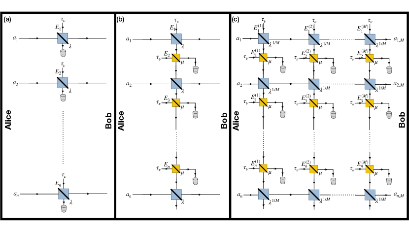
Figure 2: Interferometric representation of the $n$-mode quantum channels which describe the transmission of e.m. pulses along an optical fibre of single-signal transmissivity $\lambda$ and local temperature $\nu$ for different memory configurations. Panel (a) memoryless regime: here each one of the input modes $a_{1}$, $a_{2}$, $\cdots$, $a_{n}$ evolves independently from the others, undergoing to the same thermal attenuation mapping $\mathcal{E}_{\lambda,\nu}$ induced by beam splitter couplings (1) with the local thermal state $\tau_{\nu}$ of the local environments $E_{1}$, $E_{2}$, $\cdots$, $E_{n}$. Panel (b) LIM channel $\Phi_{\lambda,\mu,\nu}^{(1,n)}$: in this case signal cross-talks are mediated by the yellow beam splitters of transmissivity $\mu$. These allow the photons lost by the $i$th input mode to emerge in the output of the subsequent ones by letting them to interfere with the local bath $E_{i+1}$, $E_{i+2}$, $\cdots$, $E_{n}$. Setting $\mu=0$ the LIM reduces to the memoryless case of panel (a), i.e. $\Phi_{\lambda,0,\nu}^{(1,n)}=\mathcal{E}_{\lambda,\nu}^{\otimes n}$. Panel (c) DIM channel $\Phi_{\lambda,\mu,\nu}^{(M,n)}$: the fibre is described by the concatenation (4) of $M$ LIM channels $\Phi_{\lambda^{1/M},\mu,\nu}^{(1,n)}$ of transmissivity $\lambda^{1/M}$. In the Heisenberg representation, $\Phi_{\lambda,\mu,\nu}^{(M,n)}$ maps the annihilation operator $a_{i}$ (depicted on the left) of the $i$th input signal into the annihilation operators $a_{i,M}$ (depicted on the right) of the $i$th output signal for all $i=1,2,\ldots,n$. For $j=1,\cdots,M$, the symbols $E^{(j)}_{1}$, $E^{(j)}_{2}$, $\cdots$, $E^{(j)}_{n}$ represent the single-mode environments associated with the $j$th infinitesimal optical fibre element: all of them are initialised in the same thermal state $\tau_{\nu}$. Supplementary VII presents a generalisation of DIM where memoryless attenuation along the fibre occurs, concurrently with the memory effects.

More specifically, considering that for a spatially homogeneous fibre the single-signal transmissivity $\lambda$ is exponentially decreasing in the length $L$, to each of the $M$ infinitesimal components of the fibre we can assign an effective single-signal transmissivity $\lambda^{1/M}$. Their individual LIM channel representations are given by maps $\Phi_{\lambda^{1/M},\mu,\nu}^{(1,n)}$, each of which is characterised by the same local temperature parameter $\nu$ and by the same memory parameter $\mu$ of the global fibre. Similarly to the cascade construction of Giova_Palma_Master_Equations_2012 for fixed $M$, the resulting input-output DIM map is hence provided by the $M$-fold concatenation

$$\Phi_{\lambda,\mu,\nu}^{(M,n)}=\left(\Phi_{\lambda^{1/M},\mu,\nu}^{(1,n)}\right)^{M}\coloneqq\underbrace{\Phi_{\lambda^{1/M},\mu,\nu}^{(1,n)}\circ\cdots\circ\Phi_{\lambda^{1/M},\mu,\nu}^{(1,n)}}_{M}\;,$$ (4)

whose interferometric representation in terms of beam splitter couplings is given in Fig. 2(c). Note that as for LIM, the present scheme reduces to the most common model of memoryless optical fibre when the memory parameter $\mu$ vanishes: indeed, if $\mu=0$ each of the $M$ infinitesimal optical fibres can be modelled as a thermal attenuator $\mathcal{E}_{\lambda^{1/M},\nu}$ of transmissivity $\lambda^{1/M}$, and (4) gives $\Phi_{\lambda,0,\nu}^{(M,n)}=\mathcal{E}_{\lambda,\nu}$. If $\mu>0$, instead, then the environments $E_{i}^{(j)}$ are not always in the thermal state $\tau_{\nu}$, and their state depends on all previous input signals — the model exhibits memory effects.

As shown in Theorem S8 in the Supplementary, for $M\to\infty$ the mapping $\Phi_{\lambda,\mu,\nu}^{(M,n)}$ converges to an $n$-mode quantum channel denoted by $\Phi_{\lambda,\mu,\nu}^{(n)}$. The mathematically precise sense in which this convergence happens involves the notion of strong convergence, discussed in the Methods. The family of quantum channels $\{\Phi_{\lambda,\mu,\nu}^{(n)}\}_{n\in\mathds{N}}$, which forms a quantum memory channel memory-review , characterises our model of optical fibre with memory effects. Most importantly, contrary to the LIM of Ref. Memory1 ; Memory2 ; Memory3 ; Die-Hard-2-PRA ; Die-Hard-2-PRL , the map $\Phi_{\lambda,\mu,\nu}^{(n)}$ satisfies the above Properties 1–2. The proof of this fact is rather technical; the interested reader can find it in Sec. III of the Supplementary.

.2 Capacities of the model

Let $Q(\lambda,\mu,\nu)$, $Q_{2}(\lambda,\mu,\nu)$, and $K(\lambda,\mu,\nu)$ be the quantum capacity, two-way quantum capacity, and secret key capacity, respectively, of the DIM quantum memory channel $\{\Phi_{\lambda,\mu,\nu}^{(n)}\}_{n\in\mathds{N}}$. The forthcoming Theorem 1, which is proved in Theorem S14 in the Supplementary, provides conditions on the parameter region where these capacities are strictly positive. In particular, it states that one can make the capacities strictly positive by sufficiently increasing the value of $\mu$, for all nonzero values of the transmissivity $\lambda$, and all thermal photon numbers $\nu$.

Theorem 1.

Let $\lambda\in(0,1)$ and $\mu\in[0,1)$. In the absence of thermal noise, i.e. $\nu=0$, it holds that

$$Q(\lambda,\mu,\nu=0)>0\,\Longleftrightarrow\,\sqrt{\mu}>\frac{\log_{2}\left(\frac{1}{\lambda}\right)-1}{\log_{2}\left(\frac{1}{\lambda}\right)+1}\,.$$ (5)

In addition, for all $\nu\geq 0$ it holds that

$$K(\lambda,\mu,\nu),\,Q_{2}(\lambda,\mu,\nu)>0\,\Longleftrightarrow \sqrt{\mu}>\frac{\ln\left(\frac{1}{\lambda}\right)-\ln(1+\frac{1}{\nu})}{\ln\left(\frac{1}{\lambda}\right)+\ln(1+\frac{1}{\nu})}\,.$$ (6)

The following theorem, reported and proved in Theorem S15 in the Supplementary, provides the exact solution for the capacities in the absence of thermal noise.

Theorem 2.

Let $\lambda\in(0,1)$ and $\mu\in[0,1)$. In absence of thermal noise, i.e. $\nu=0$, it holds that

$$Q\left(\lambda,\mu,\nu=0\right) =\int_{0}^{2\pi}\frac{\mathrm{d}x}{2\pi}\,\max\left\{0,\log_{2}\left(\frac{\eta^{(\lambda,\mu)}(x)}{1-\eta^{(\lambda,\mu)}(x)}\right)\right\}\,,$$ (7)

$$Q_{2}\left(\lambda,\mu,\nu=0\right) =K\left(\lambda,\mu,\nu=0\right)$$

$$=\int_{0}^{2\pi}\frac{\mathrm{d}x}{2\pi}\,\log_{2}\left(\frac{1}{1-\eta^{(\lambda,\mu)}(x)}\right)\,,$$

where

$$\eta^{(\lambda,\mu)}(x)\coloneqq\lambda^{\frac{1-\mu}{1+\mu-2\sqrt{\mu}\cos(x/2)}}\quad\forall\,x\in[0,2\pi]\,.$$ (8)

In Fig. 3, we plot the capacities given in (7). If $\mu=0$ (i.e. in the memoryless case), all these capacities are equal to the corresponding capacities of the pure-loss channel. Upon plotting the capacities in Fig. 3, one observes that for any $\lambda\in(0,1]$ all the capacities $Q\left(\lambda,\mu,\nu=0\right)$, $Q_{2}\left(\lambda,\mu,\nu=0\right)$, and $K\left(\lambda,\mu,\nu=0\right)$ are monotonically increasing in $\mu\in[0,1]$. Hence, at least in the absence of thermal noise, as the memory parameter $\mu$ increases (corresponding to a decrease in the time interval between consecutive signals), quantum communication performances improve. It is reasonable to expect that such a monotonicity in $\mu$ holds even for $\nu>0$.

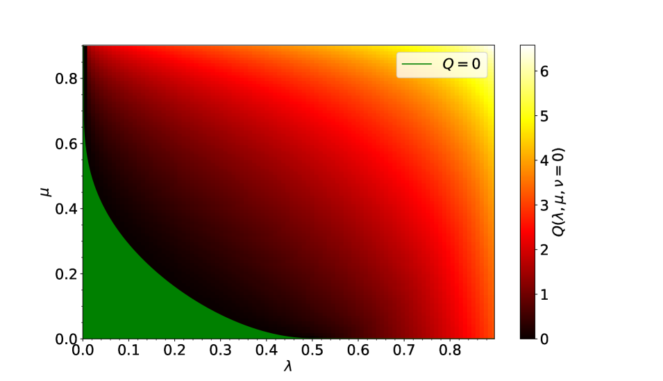
(a)

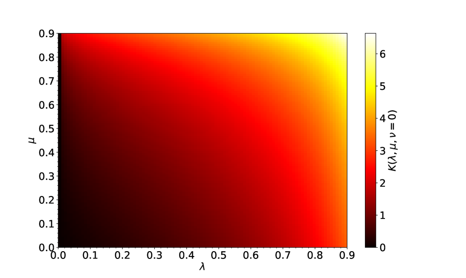
(b)

Figure 3: In (a) we plot the quantum capacity $Q(\lambda,\mu,\nu=0)$ of the quantum memory channel $\{\Phi^{(n)}_{\lambda,\mu,\nu=0}\}_{n\in\mathds{N}}$ with respect to $\lambda,\mu\in[0,0.9]$ for $\nu=0$. The green region is the one where the quantum capacity vanishes, which is is given by all the points $(\lambda,\mu)$ such that $\sqrt{\mu}\leq\frac{\log_{2}\left(\frac{1}{\lambda}\right)-1}{\log_{2}\left(\frac{1}{\lambda}\right)+1}$, as established by Theorem 1.    In (b) we plot the secret-key capacity $K(\lambda,\mu,\nu=0)$ of the quantum memory channel $\{\Phi^{(n)}_{\lambda,\mu,\nu=0}\}_{n\in\mathds{N}}$ with respect to $\lambda,\mu\in[0,0.9]$ for $\nu=0$. This capacity is exactly equal to the two-way quantum capacity $Q_{2}(\lambda,\mu,\nu=0)$, as guaranteed by Theorem 2.    The capacities plotted in (a) and in (b) are calculated by exploiting the expressions given in (7). In (a) and in (b) we have limited the range of $\lambda$ and $\mu$ to the interval $[0,0.9]$ because all the capacities $Q$, $Q_{2}$, and $K$ diverge when either $\lambda$ or $\mu$ approaches $1$.

Discussion

In this paper we analysed quantum communication, entanglement distribution, and quantum key distribution across optical fibres in the little-studied case where memory effects are present, and hence commonly employed approximations break down. It is generally believed that memory effects should improve the information transfer of a communication line, by offering a means to recover potentially lost information that would otherwise be unrecoverable in a memoryless scenario. Indeed, in a memoryless scenario, if photons are lost, they are irretrievably gone. However, in the presence of memory effects, there exists a probability that lost photons can interact with subsequent signals, allowing some information encoded in lost photons to persist within the fibre.

We first proposed a model of optical fibre with memory effects which overcomes problems of the LIM previously introduced in the literature Memory1 ; Memory2 ; Memory3 ; Die-Hard-2-PRA ; Die-Hard-2-PRL . Our model depends on three parameters: the transmissivity $\lambda\in[0,1]$ of the optical fibre, the thermal noise $\nu\geq 0$, and the memory parameter $\mu\in[0,1]$, with the latter being related to the time interval between subsequent signals. In particular, increasing $\mu$ has the operational meaning as a decrease in the time interval between subsequent signals.

In Theorem 2 we found the exact solution for the quantum capacity $Q$, the two-way quantum capacity $Q_{2}$, and the secret-key capacity $K$ of the DIM channel in the absence of thermal noise ($\nu=0$). These capacities are monotonically increasing in the memory parameter $\mu$, meaning that memory effects improve quantum communication. It is worth noting that in the presence of thermal noise ($\nu>0$) the capacities remain unknown even in the absence of memory effects ($\mu=0$), as the capacities of the thermal attenuator are currently unknown.

The reader might question the meaningfulness of considering communication tasks assisted by two-way classical communication in a setting where the memory parameter $\mu$, and thus the time interval between subsequent signals, is fixed. Indeed, in general, the rounds of classical communication between consecutive channel uses may vary during the communication protocol. Additionally, another problem is that, when the sender and receiver are very far apart, even a single round of classical communication requires an excessively long waiting time which prevents the exploitation of memory effects altogether. However, in the case of Choi-simulable channels PLOB , it is meaningful to consider such communication tasks. This is because optimal entanglement and secret-key distribution strategies for Choi-simulable channels can be achieved by initially utilising the channel (with a constant and short time interval between subsequent input signals) to share multiple copies of the Choi state, followed by employing optimal distillation protocols (either for entanglement or secret-key) to distil the Choi state. Fortunately, our model is associated with the quantum memory channel $\{\Phi_{\lambda,\mu,\nu}^{(n)}\}_{n\in\mathds{N}}$, which is Choi simulable because it is Gaussian PLOB .

In the absence of memory effects ($\mu=0$), it is known that no quantum communication tasks can be achieved when the transmissivity is sufficiently low ($Q=0$ for $\lambda\leq\frac{1}{2}$, and $Q_{2}=K=0$ for $\lambda\leq\frac{\nu}{\nu+1}$). However, in Theorem 1 we established that for any transmissivity $\lambda>0$ and thermal noise $\nu\geq 0$, there exists a critical value of the memory parameter $\mu$ above which it becomes possible to achieve qubit distribution ($Q>0$), entanglement distribution ($Q_{2}>0$), and secret-key distribution ($K>0$). This result is particularly intriguing as it demonstrates that — at least within our model — memory effects provide an advantage, enabling quantum communication tasks to be performed in highly noisy regimes where it was previously considered impossible without the use of quantum repeaters. While this result is model dependent, it offers hope that memory effects could offer a concrete route to achieve efficient long-distance quantum communication with fewer quantum repeaters than previously believed. Specifically, this result bears resemblance to the “die-hard quantum communication” effect" observed in Die-Hard-2-PRL ; Die-Hard-2-PRA within their toy model of optical fibre with memory effects, which was limited to the analysis of $Q$ only and does not consider $K$ and $Q_{2}$. In our paper, we not only demonstrate the persistence of such an effect in a more realistic model, accounting for $Q$, $Q_{2}$, and $K$, but we also derive an analytical expression for the critical value of the memory parameter $\mu$, which goes beyond the findings of Die-Hard-2-PRL ; Die-Hard-2-PRA . Note that, by relating $\mu$ to the temporal interval $\delta t$ between subsequent input signals (e.g. $\mu=e^{-\delta t/t_{E}}$ with $t_{E}$ being the thermalisation timescale), Theorem 1 can also be expressed in terms of the critical $\delta t$ below which the above mentioned quantum communication tasks can be achieved.

Acknowledgements — FAM and VG acknowledge financial support by MUR (Ministero dell’Istruzione, dell’Università e della Ricerca) through the following projects: PNRR MUR project PE0000023-NQSTI, PRIN 2017 Taming complexity via Quantum Strategies: a Hybrid Integrated Photonic approach (QUSHIP) Id. 2017SRN-BRK, and project PRO3 Quantum Pathfinder. GDP has been supported by the HPC Italian National Centre for HPC, Big Data and Quantum Computing - Proposal code CN00000013 and by the Italian Extended Partnership PE01 - FAIR Future Artificial Intelligence Research - Proposal code PE00000013 under the MUR National Recovery and Resilience Plan funded by the European Union - NextGenerationEU. GDP is a member of the “Gruppo Nazionale per la Fisica Matematica (GNFM)” of the “Istituto Nazionale di Alta Matematica “Francesco Severi” (INdAM)”. MF is supported by a Juan de la Cierva Formaciòn fellowship (project FJC2021-047404-I), with funding from MCIN/AEI/10.13039/501100011033 and European Union NextGenerationEU/PRTR, and by Spanish Agencia Estatal de Investigaciòn, project PID2019-107609GB-I00/AEI/10.13039/501100011033, by the European Union Regional Development Fund within the ERDF Operational Program of Catalunya (project QuantumCat, ref. 001-P-001644), and by European Space Agency, project ESA/ESTEC 2021-01250-ESA. FAM and LL thank the Freie Universität Berlin for hospitality. FAM, LL, and VG acknowledge valuable discussions with Paolo Villoresi, Giuseppe Vallone, and Marco Avesani and their hospitality at the University of Padua. FAM and MF acknowledge valuable discussions with Giovanni Barbarino regarding the Avram–Parter theorem and Szegő theorem.

Supplementary Information is available for this paper.

Competing interest — The authors declare no competing interests.

Methods

Let $\pazocal{H}$ be an Hilbert space, let $\mathcal{L}(\pazocal{H})$ the space of linear operators on $\pazocal{H}$, and let $\mathfrak{S}(\pazocal{H})$ be the set of quantum states on $\pazocal{H}$. Given a quantum channel $\Phi$ and a sequence of quantum channels $\{\Phi_{k}\}_{k\in\mathds{N}}$, we say that $\{\Phi_{k}\}_{k\in\mathds{N}}$ strongly converges to $\Phi$ if

$$\lim\limits_{k\to\infty}\|\Phi_{k}(\rho)-\Phi(\rho)\|_{1}=0\quad\forall\,\rho\in\mathfrak{S}(\pazocal{H})\,,$$ (9)

where $\|\Theta\|_{1}\coloneqq\operatorname{Tr}\sqrt{\Theta^{\dagger}\Theta}$ denotes the trace norm of a linear operator $\Theta$. We now define quantum memoryless and memory channels, and introduce relevant notations.

Definition 1.

Let $\{\Phi^{(n)}\}_{n\in\mathds{N}}$ be a family of quantum channels with $\Phi^{(n)}:\mathcal{L}(\pazocal{H}^{\otimes n})\to\mathcal{L}(\pazocal{H}^{\otimes n})$ for all $n\in\mathds{N}$. The family $\{\Phi^{(n)}\}_{n\in\mathds{N}}$ is memoryless if there exists a quantum channel $\Phi:\mathcal{L}(\pazocal{H})\to\mathcal{L}(\pazocal{H})$ such that $\Phi^{(n)}=\Phi^{\otimes n}$ for all $n\in\mathds{N}$. In such a scenario, we will also refer to $\Phi$ as a memoryless channel. Moreover, given a capacity $C$ (e.g. $C\in\{Q,Q_{2},K\}$), the capacity $C$ of the memoryless quantum channel $\Phi$ is denoted as $C(\Phi)$.

Definition 2.

Let $\{\Phi^{(n)}\}_{n\in\mathds{N}}$ be a family of quantum channels with $\Phi^{(n)}:\mathcal{L}(\pazocal{H}^{\otimes n})\to\mathcal{L}(\pazocal{H}^{\otimes n})$ for all $n\in\mathds{N}$. The family $\{\Phi^{(n)}\}_{n\in\mathds{N}}$ is a memory quantum channel if it is not memoryless. In such a scenario, the term "$n$ channel uses" corresponds to the quantum channel $\Phi^{(n)}$. Moreover, given a capacity $C$ (e.g. $C\in\{Q,Q_{2},K\}$), the capacity $C$ of the quantum memory channel $\{\Phi^{(n)}\}_{n\in\mathbb{N}}$ is denoted as $C\left(\{\Phi^{(n)}\}_{n\in\mathbb{N}}\right)$.

For all $\lambda\in[0,1]$ the capacities $Q$ holwer ; LossyECEAC1 ; LossyECEAC2 , $Q_{2}$ PLOB , and $K$ PLOB of the pure-loss channel $\mathcal{E}_{\lambda,0}$ are given by:

$$Q(\mathcal{E}_{\lambda,0}) =\begin{cases}\log_{2}\left(\frac{\lambda}{1-\lambda}\right)&\text{if $\lambda\in[\frac{1}{2},1]$ ,}\\ 0&\text{if $\lambda\in[0,\frac{1}{2}]$ .}\end{cases}$$ (10)

$$Q_{2}(\mathcal{E}_{\lambda,0}) =K(\mathcal{E}_{\lambda,0})=\log_{2}\left(\frac{1}{1-\lambda}\right)\,.$$

In the following we will outline the key concepts that enabled us to derive the results stated in Section .2. To achieve this, we generalise methods introduced in Memory1 ; Memory2 ; Memory3 . Let us begin with the forthcoming Theorem 3, which is proved in Theorem S8 in the Supplementary.

Theorem 3.

Let $\lambda,\mu\in[0,1]$, $\nu\geq 0$, and $n\in\mathds{N}$. There exists passive BUCCO $n$-mode unitary transformations $\mathcal{U}_{1},\mathcal{U}_{2}$ such that

$$\mathcal{U}_{2}\circ\Phi_{\lambda,\mu,\nu}^{(n)}\circ\mathcal{U}_{1}=\bigotimes_{i=1}^{n}\mathcal{E}_{\eta_{i}^{(n,\lambda,\mu)},\nu}\,,$$ (11)

where the transmissivities $\{\eta_{i}^{(n,\lambda,\mu)}\}_{i=1,2,\ldots,n}$ are the square of the singular values, indexed in increasing order, of the $n\times n$ real matrix $\bar{A}^{(n,\lambda,\mu)}$ whose $(i,k)$ element is

$$\bar{A}^{(n,\lambda,\mu)}_{i,k}\coloneqq\Theta(i-k)\,\sqrt{\lambda}\mu^{\frac{i-k}{2}}L_{i-k}^{(-1)}(-\ln\lambda)$$ (12)

for all $i,k\in\{1,2,\ldots,n\}$. Here, $L_{m}^{(-1)}$ is a generalised Laguerre polynomial, and

$$\Theta(x)\coloneqq\begin{cases}1,&\text{if $x\geq 0$,}\\ 0,&\text{otherwise.}\end{cases}$$ (13)

Consequently, any capacity of the quantum memory channel $\{\Phi_{\lambda,\mu,\nu}^{(n)}\}_{n\in\mathds{N}}$ coincides with the corresponding capacity of $\{\bigotimes_{i=1}^{n}\mathcal{E}_{\eta_{i}^{(n,\lambda,\mu)},\nu}\}_{n\in\mathds{N}}$.

The proof of (11) involves expressing the output annihilation operators $\{a_{i,M}\}_{i=1,2,\ldots,n}$ (see Figure 2) in terms of the input ones $\{a_{i}\}_{i=1,2,\ldots,n}$, performing a Bogoliubov transformation, and finally taking the continuum limit $M\to\infty$. As a consequence of (11), the quantum memory channel $\Phi_{\lambda,\mu,\nu}^{(n)}$, which models $n$ uses of the optical fibre, is unitarily equivalent to a tensor product of $n$ distinct thermal attenuators. Consequently, if Alice and Bob are linked by $\Phi_{\lambda,\mu,\nu}^{(n)}$ (resp. $\bigotimes_{i=1}^{n}\mathcal{E}_{\eta_{i}^{(n,\lambda,\mu)},\nu}$), they can simulate $\bigotimes_{i=1}^{n}\mathcal{E}_{\eta_{i}^{(n,\lambda,\mu)},\nu}$ (resp. $\Phi_{\lambda,\mu,\nu}^{(n)}$) through the application of $\mathcal{U}_{1}$ (resp. $\mathcal{U}_{1}^{\dagger}$) by Alice just before transmission, and $\mathcal{U}_{2}$ (resp. $\mathcal{U}_{2}^{\dagger}$) by Bob just after reception. This implies the capacity equivalence between $\{\Phi_{\lambda,\mu,\nu}^{(n)}\}_{n\in\mathds{N}}$ and $\{\bigotimes_{i=1}^{n}\mathcal{E}_{\eta_{i}^{(n,\lambda,\mu)},\nu}\}_{n\in\mathds{N}}$, as stated in the final part of Theorem 3. Notably, this equivalence holds even for energy-constrained capacities memory-review , thanks to the passivity of $\mathcal{U}_{1}$.

Let us analyse the behaviour of the transmissivities $\{\eta_{i}^{(n,\lambda,\mu)}\}_{i=1,2,\ldots,n}$, as the number of uses of the optical fibre, $n$, approaches infinity. By plotting in Fig. 4 the points

$$\left\{\left(2\pi\frac{j}{n}\,,\,\eta_{j}^{(n,\lambda,\mu)}\right)\,:\,j=1,2,\ldots,n\right\}$$ (14)

on a two-dimensional plane, we observe that they converge for $n\to\infty$ to the graph of a function $\eta^{(\lambda,\mu)}:[0,2\pi]\to\mathbb{R}$, which we dub effective transmissivity function. We formally state this result in the forthcoming Theorem 4 and we provide its proof in Theorem S13 in the Supplementary by establishing a corollary of the Avram–Parter theorem Avram1988 ; Parter1986 , a matrix analysis result about the asymptotic behaviour for $n\to\infty$ of the singular values of a $n\times n$ Toeplitz matrix. Notably, our corollary, reported in Theorem S12 in the Supplementary, seems to be unknown in the matrix analysis literature and we believe it may have independent interest.

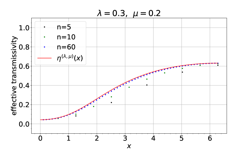
Figure 4: The red curve is the effective transmissivity function $\eta^{(\lambda,\mu)}(x)$, as defined in (16), plotted with respect $x\in[0,2\pi]$ for $\lambda=0.3$ and $\mu=0.2$. For $n=4$ (black points), $n=10$ (green points), and $n=60$ (blue points), we plot the $n$ points $\left\{\left(2\pi\frac{j}{n}\,,\,\eta_{j}^{(n,\lambda,\mu)}\right)\,:\,j=1,2,\ldots,n\right\}$. We observe that these $n$ points converge for $n\rightarrow\infty$ to the graph of the effective transmissivity function $\eta^{(\lambda,\mu)}$, as established by Theorem 4. Here, $\{\eta_{j}^{(n,\lambda,\mu)}\}_{j=1,2,\ldots,n}$ are the transmissivities defined in Theorem 3.

Theorem 4.

Let $\lambda\in[0,1]$ and $\mu\in[0,1)$. There exists a sequence $\{j_{n}\}_{n\in\mathds{N}}\subseteq\mathds{N}$ such that $0\leq j_{n}\leq n$ for all $n\in\mathds{N}$, $\lim\limits_{n\rightarrow\infty}\frac{j_{n}}{n}=0$, and

$$\lim\limits_{n\rightarrow\infty}\max\left\{\left|\eta^{(n,\lambda,\mu)}_{j}-\eta^{(\lambda,\mu)}\left(\frac{2\pi j}{n}\right)\right|:\,j\in\{j_{n},\ldots,n\}\right\}=0\,,$$ (15)

where the effective transmissivity function is defined as

$$\eta^{(\lambda,\mu)}(x)\coloneqq\lambda^{\frac{1-\mu}{1+\mu-2\sqrt{\mu}\cos(x/2)}}\quad\forall\,x\in[0,2\pi]\,.$$ (16)

As a consequence of the previous theorem and the fact that $\max_{x\in[0,2\pi]}\eta^{(\lambda,\mu)}(x)=\eta^{(\lambda,\mu)}(2\pi)$, the value $\eta^{(\lambda,\mu)}(2\pi)$ determines whether or not the capacities of our model are strictly positive. Hence, (2) and (3) imply the following theorem, which is proved in Theorem S14 in the Supplementary.

Theorem 5.

Let $\lambda\in(0,1)$, $\mu\in[0,1)$, and $\nu\geq 0$. Let $C(\lambda,\mu,\nu)$ be one of the following capacities of the quantum memory channel $\{\Phi_{\lambda,\mu,\nu}^{(n)}\}_{n\in\mathds{N}}$: quantum capacity $Q$, two-way quantum capacity $Q_{2}$, or secret key capacity $K$. It holds that

$$C(\lambda,\mu,\nu)>0\,\Longleftrightarrow\,C(\mathcal{E}_{\eta^{(\lambda,\mu)}(2\pi),\nu})>0\,,$$ (17)

where $\eta^{(\lambda,\mu)}$ is reported in (16). In particular, in the absence of thermal noise, i.e. $\nu=0$, it holds that

$$Q(\lambda,\mu,\nu=0)>0\,\Longleftrightarrow\,\sqrt{\mu}>\frac{\log_{2}\left(\frac{1}{\lambda}\right)-1}{\log_{2}\left(\frac{1}{\lambda}\right)+1}\,.$$ (18)

In addition, for all $\nu\geq 0$ it holds that

$$K(\lambda,\mu,\nu),\,Q_{2}(\lambda,\mu,\nu)>0\,\Longleftrightarrow \sqrt{\mu}>\frac{\ln\left(\frac{1}{\lambda}\right)-\ln(1+\frac{1}{\nu})}{\ln\left(\frac{1}{\lambda}\right)+\ln(1+\frac{1}{\nu})}\,.$$ (19)

Now, let us provide a brief overview of the key ideas underlying the derivation of the capacities of $\{\bigotimes_{i=1}^{n}\mathcal{E}_{\eta_{i}^{(n,\lambda,\mu)},\nu}\}_{n\in\mathds{N}}$. For additional technical details, see Theorem S15 in the Supplementary. For $l,P\in\mathds{N}$, consider $Pl$ channel uses as divided into $P\rightarrow\infty$ groups, each containing $l\rightarrow\infty$ channel uses:

$$\bigotimes_{i=1}^{lP}\mathcal{E}_{\eta_{i}^{(Pl,\lambda,\mu)},\nu}=\bigotimes_{j=1}^{l}\bigotimes_{p=1}^{P}\mathcal{E}_{\eta_{(p-1)l+j}^{(Pl,\lambda,\mu)},\nu}\,.$$ (20)

Roughly speaking, Theorem 4 implies that for any $j\in\{1,2,\ldots,l\}$ it holds that

$$\eta_{(p-1)l+j}^{(Pl,\lambda,\mu)}\simeq\eta^{(\lambda,\mu)}\left(2\pi\frac{p}{P}\right)\quad\text{for $l,P\to\infty$}\,,$$ (21)

meaning that $lP$ channel uses, with $l,P\to\infty$, corresponds to $l$ uses of the following $P$-mode thermal attenuator:

$$\bigotimes_{p=1}^{P}\mathcal{E}_{\eta^{(\lambda,\mu)}(2\pi\frac{p}{P}),\nu}\,,$$ (22)

which is a memoryless quantum channel. Hence, for any capacity $C$ (e.g. $C=Q,Q_{2},K$) it holds that the capacity $C$ of the quantum memory channel $\{\Phi_{\lambda,\mu,\nu}^{(n)}\}_{n\in\mathds{N}}$ satisfies

$$C\left(\{\Phi_{\lambda,\mu,\nu}^{(n)}\}_{n\in\mathds{N}}\right) \overset{\text{(i)}}{\approx}\lim\limits_{P\rightarrow\infty}\frac{1}{P}C\left(\bigotimes_{p=1}^{P}\mathcal{E}_{\eta^{(\lambda,\mu)}(2\pi\frac{p}{P}),\nu}\right)$$ (23)

$$\stackrel{{\scriptstyle\mathclap{\scriptsize\mbox{(ii)}}}}{{\geq}}\lim\limits_{P\rightarrow\infty}\frac{1}{P}\sum_{p=1}^{P}C\left(\mathcal{E}_{\eta^{(\lambda,\mu)}(2\pi\frac{p}{P}),\nu}\right)$$ (24)

$$\stackrel{{\scriptstyle\mathclap{\scriptsize\mbox{(iii)}}}}{{=}}\int_{0}^{2\pi}\frac{\mathrm{d}x}{2\pi}\,C\left(\mathcal{E}_{\eta^{(\lambda,\mu)}(x),\nu}\right)\,,$$ (25)

where: (i) comes from the fact that a single use of the $P$-mode attenuator in (22) is approximately equivalent to $P$ uses of the optical fibre; (ii) is a consequence of the fact that Alice and Bob can independently employ the optimal communication strategy for each of the $P$ single-mode channels that define the $P$-mode attenuator; in (iii) we have just introduced the Riemann integral. Moreover, the equality in (24) holds if $C$ is additive, i.e. if $C$ is such that for all transmissivities $\{\lambda_{p}\}_{p=1,2,\ldots,P}$ and all $P\in\mathds{N}$ it holds that

$$C\left(\bigotimes_{p=1}^{P}\mathcal{E}_{\lambda_{p},\nu}\right)=\sum_{p=1}^{P}C\left(\mathcal{E}_{\lambda_{p},\nu}\right)\,.$$ (26)

Hence, leveraging the additivity and the expression in (10) of the capacities $Q$ Wolf2007 , $Q_{2}$ PLOB , and $K$ PLOB of the pure-loss channel, we can derive the precise values of the capacities of our model in the absence of thermal noise. This exact solution is provided by Theorem 6, which is proved in Theorem S15 in the Supplementary.

Theorem 6.

Let $\lambda\in(0,1)$, $\mu\in[0,1)$, $\nu\geq 0$. Let $C$ be one of the following capacities: quantum capacity $Q$, two-way quantum capacity $Q_{2}$, or secret key capacity $K$. In addition, let $C(\lambda,\mu,\nu)$ be the capacity $C$ of the quantum memory channel $\{\Phi_{\lambda,\mu,\nu}^{(n)}\}_{n\in\mathds{N}}$. In absence of thermal noise, i.e. $\nu=0$, it holds that

$$C(\lambda,\mu,\nu=0)=\int_{0}^{2\pi}\frac{\mathrm{d}x}{2\pi}\,C\left(\mathcal{E}_{\eta^{(\lambda,\mu)}(x),0}\right)\,.$$ (27)

where $\eta^{(\lambda,\mu)}(x)$ is the effective transmissivity function expressed in (16). In particular,

$$Q\left(\lambda,\mu,\nu=0\right) =\int_{0}^{2\pi}\frac{\mathrm{d}x}{2\pi}\,\max\left\{0,\log_{2}\left(\frac{\eta^{(\lambda,\mu)}(x)}{1-\eta^{(\lambda,\mu)}(x)}\right)\right\}\,,$$ (28)

$$Q_{2}\left(\lambda,\mu,\nu=0\right) =K\left(\lambda,\mu,\nu=0\right)$$

$$=\int_{0}^{2\pi}\frac{\mathrm{d}x}{2\pi}\,\log_{2}\left(\frac{1}{1-\eta^{(\lambda,\mu)}(x)}\right)\,.$$

Moreover, in the presence of thermal noise, i.e. $\nu>0$, it holds that

$$C(\lambda,\mu,\nu)\geq\int_{0}^{2\pi}\frac{\mathrm{d}x}{2\pi}C\left(\mathcal{E}_{\eta^{(\lambda,\mu)}(x),\nu}\right)\,.$$ (29)

Notation and preliminaries

Let $\pazocal{H}$ be an Hilbert space, let $\mathcal{L}(\pazocal{H})$ the space of linear operators on $\pazocal{H}$, and let $\mathfrak{S}(\pazocal{H})$ be the set of quantum states on $\pazocal{H}$. The trace norm of a linear operator $\Theta$ is defined by $\|\Theta\|_{1}\coloneqq\operatorname{Tr}\sqrt{\Theta^{\dagger}\Theta}$. A map $\Phi:\mathcal{L}(\pazocal{H})\to\mathcal{L}(\pazocal{H})$ is a quantum channel if it is linear, completely positive, and trace preserving. Given a quantum channel $\Phi$ and a sequence of quantum channels $\{\Phi_{k}\}_{k\in\mathds{N}}$, we say that $\{\Phi_{k}\}_{k\in\mathds{N}}$ strongly converges to $\Phi$ when

$$\lim\limits_{k\to\infty}\|\Phi_{k}(\rho)-\Phi(\rho)\|_{1}=0\quad\forall\,\rho\in\mathfrak{S}(\pazocal{H})\,.$$ (S1)

We now define quantum memoryless and memory channels, and introduce relevant notations.

Definition 3.

Let $\{\Phi^{(n)}\}_{n\in\mathds{N}}$ be a family of quantum channels with $\Phi^{(n)}:\mathcal{L}(\pazocal{H}^{\otimes n})\to\mathcal{L}(\pazocal{H}^{\otimes n})$ for all $n\in\mathds{N}$. The family $\{\Phi^{(n)}\}_{n\in\mathds{N}}$ is memoryless if there exists a quantum channel $\Phi:\mathcal{L}(\pazocal{H})\to\mathcal{L}(\pazocal{H})$ such that $\Phi^{(n)}=\Phi^{\otimes n}$ for all $n\in\mathds{N}$. In such a scenario, we will also refer to $\Phi$ as a memoryless channel.

Definition 4.

Let $\{\Phi^{(n)}\}_{n\in\mathds{N}}$ be a family of quantum channels with $\Phi^{(n)}:\mathcal{L}(\pazocal{H}^{\otimes n})\to\mathcal{L}(\pazocal{H}^{\otimes n})$ for all $n\in\mathds{N}$. The family $\{\Phi^{(n)}\}_{n\in\mathds{N}}$ is a memory quantum channel if it is not memoryless. In such a scenario, the term "$n$ channel uses" corresponds to the quantum channel $\Phi^{(n)}$.

Quantum information with continuous variables systems

Let us provide a brief overview of the formalism of quantum information with continuous variable systems [24]. In this context, we consider $m$ modes of harmonic oscillators denoted by $S_{1}$, $S_{2}$, $\ldots$, $S_{m}$, which are associated with the Hilbert space $L^{2}(\mathbb{R}^{m})$, which comprises all square-integrable complex-valued functions over $\mathbb{R}$. Each mode represents a single mode of electromagnetic radiation with a definite frequency and polarisation. For each $j=1,2,\ldots,m$, the annihilation operator $a_{j}$ of mode $S_{j}$ is defined as $a_{j}\coloneqq\frac{\hat{x}_{j}+i\hat{p}_{j}}{\sqrt{2}}$, where $\hat{x}_{j}$ and $\hat{p}_{j}$ are the well-known position and momentum operators of mode $S_{j}$. The operator $a_{j}^{\dagger}$ is referred to as the creation operator of mode $S_{j}$. The operator $a_{j}^{\dagger}a_{j}$ corresponds to the photon number of mode $S_{j}$. The $n$th Fock state of mode $S_{j}$ is defined as

$$\ket{n}_{S_{j}}\coloneqq\frac{(a_{j}^{\dagger})^{n}}{\sqrt{n!}}\ket{0}_{S_{j}}\,,$$ (S2)

where $\ket{0}_{S_{j}}$ represents the vacuum state of mode $S_{j}$. The characteristic function $\chi_{\rho}:\mathbb{C}^{m}\to\mathbb{C}$ of a $m$-mode state $\rho\in\mathfrak{S}(L^{2}(\mathbb{R}^{m}))$ is defined as

$$\chi_{\rho}(\alpha)\coloneqq \ \operatorname{Tr}\left[\rho D(\alpha)\right]\,,$$ (S3)

where for all $\alpha\in\mathbb{C}^{m}$ the displacement operator $D(\alpha)$ is defined as

$$D(\alpha)\coloneqq\exp\left[\sum_{j=1}^{m}(\alpha_{j}a^{\dagger}_{j}-\alpha_{j}^{*}a_{j})\right]\,.$$ (S4)

Any state $\rho$ can be written in terms of its characteristic function as

$$\rho=\ \int\frac{\mathrm{d}^{2m}\alpha}{\pi^{m}}\,\chi_{\rho}(\alpha)D(-\alpha)\,,$$ (S5)

and, consequently, quantum states and characteristic functions are in one-to-one correspondence. The following Lemma (see ([42, Lemma 4] or [43, Theorem 2])) will be useful for the following.

Lemma S7.

Let $m\in\mathds{N}$, let $\{\sigma_{k}\}_{k\in\mathds{N}}\subseteq\mathfrak{S}\left(L^{2}(\mathbb{R}^{m})\right)$ be a sequence of $m$-mode states, and let $\sigma\in\mathfrak{S}\left(L^{2}(\mathbb{R}^{m})\right)$ be a $m$-mode state. Then, $\{\sigma_{k}\}_{k\in\mathds{N}}$ converges in trace norm to $\sigma$ if and only if the sequence of characteristic functions $\{\chi_{\sigma_{k}}\}_{k\in\mathds{N}}$ converges pointwise to the characteristic function $\chi_{\sigma}$. In formula, it holds that

$$\lim\limits_{k\to\infty}\|\sigma_{k}-\sigma\|_{1}=0\qquad\Longleftrightarrow\qquad\lim\limits_{k\to\infty}\chi_{\sigma_{k}}(\alpha)=\chi_{\sigma}(\alpha)\quad\forall\,\alpha\in\mathbb{C}\,.$$ (S6)

Remark 1.

Let us consider $m$ single-mode systems with annihilation operators $a_{1},a_{2},\ldots,a_{m}$ and let us define the following vector of annihilation operators:

$$\textbf{a}\coloneqq(a_{1},a_{2},\ldots,a_{m})^{T}\,.$$ (S7)

For any $n\times n$ orthogonal matrix $O$ one can define a unitary operator $U_{O}$ on $L^{2}(\mathbb{R})^{\otimes m}$ such that $U_{O}^{\dagger}\mathbf{a}U_{O}=O\mathbf{a}$. The transformation $\mathcal{U}_{O}(\cdot)\coloneqq U_{O}\cdot U_{O}^{\dagger}$ is dubbed "passive" [24] and it preserves the total photon number, i.e.

$$U_{O}^{\dagger}\left(\sum_{j=1}^{m}a_{j}^{\dagger}a_{j}\right)U_{O}=\sum_{j=1}^{m}a_{j}^{\dagger}a_{j}\,.$$ (S8)

Note that, at the level of characteristic functions, for any quantum state $\rho\in\mathfrak{S}\left(L^{2}(\mathbb{R}^{m})\right)$ it holds that

$$\chi_{\mathcal{U}_{O}(\rho)}(\alpha)=\chi_{\rho}(O^{T}\alpha)\qquad\forall\,\alpha\in\mathbb{C}^{m}\,.$$ (S9)

.3 Beam splitter and thermal attenuator

Let $\pazocal{H}_{S}$ and $\pazocal{H}_{E}$ be single-mode systems and let $a$ and $b$ denote their annihilation operators, respectively. For all $\lambda\in[0,1]$ the unitary operator describing a beam splitter of transmissivity $\lambda$ is

$$U_{\lambda}^{SE}\coloneqq\exp\left[\arccos\sqrt{\lambda}\left(a^{\dagger}b-a\,b^{\dagger}\right)\right]\,.$$ (S10)

Under the beam splitter unitary, the annihilation operators $a$ and $b$ transform as

$$\left(U_{\lambda}^{SE}\right)^{\dagger}a\,U_{\lambda}^{SE} =\sqrt{\lambda}\,a+\sqrt{1-\lambda}\,b\,,$$ (S11)

$$U_{\lambda}^{SE}a\,\left(U_{\lambda}^{SE}\right)^{\dagger} =\sqrt{\lambda}\,a-\sqrt{1-\lambda}\,b\,,$$

$$\left(U_{\lambda}^{SE}\right)^{\dagger}b\,U_{\lambda}^{SE} =-\sqrt{1-\lambda}\,a+\sqrt{\lambda}\,b\,,$$

$$U_{\lambda}^{SE}b\,\left(U_{\lambda}^{SE}\right)^{\dagger} =\sqrt{1-\lambda}\,a+\sqrt{\lambda}\,b\,.$$

At the level of characteristic functions, the beam splitter transforms any two-mode state $\rho\in\mathfrak{S}(\pazocal{H}_{S}\otimes\pazocal{H}_{E})$ as

$$\chi_{U^{SE}_{\lambda}\rho U_{\lambda}^{{SE}^{\dagger}}}(\alpha,\beta)\coloneqq\operatorname{Tr}\left[U^{SE}_{\lambda}\rho U_{\lambda}^{{SE}^{\dagger}}\,D_{S}(\alpha)\otimes D_{E}(\beta)\right] =\chi_{\rho}\left(\sqrt{\lambda}\,\alpha-\sqrt{1-\lambda}\,\beta,\,\sqrt{1-\lambda}\,\alpha+\sqrt{\lambda}\,\beta\right)\qquad\alpha,\beta\in\mathbb{C}\,.$$ (S12)

For all $\lambda\in[0,1]$ and $\nu\geq 0$, a thermal attenuator $\mathcal{E}_{\lambda,\nu}:\mathfrak{S}(\pazocal{H}_{S})\to\mathfrak{S}(\pazocal{H}_{S})$ is a quantum channel defined as follows:

$$\mathcal{E}_{\lambda,\nu}(\rho)\coloneqq\operatorname{Tr}_{E}\left[U_{\lambda}^{SE}\big{(}\rho^{S}\otimes\tau_{\nu}^{E}\big{)}{U_{\lambda}^{SE}}^{\dagger}\right]\,,$$ (S13)

Here, $\tau_{\nu}\in\mathfrak{S}(\pazocal{H}_{E})$ denotes the thermal state with mean photon number equal to $\nu$, which is defined by

$$\tau_{\nu}\coloneqq\frac{1}{\nu+1}\sum_{n=0}^{\infty}\left(\frac{\nu}{\nu+1}\right)^{n}\ket{n}\!\!\bra{n}\,,$$ (S14)

and its characteristic function reads

$$\chi_{\tau_{\nu}}(\alpha)\coloneqq e^{-\frac{1}{2}(2\nu+1)|\alpha|^{2}}\quad\forall\,\alpha\in\mathbb{C}\,.$$ (S15)

By exploiting (S12) and (S15), it can be shown that the thermal attenuator transforms any single-mode state $\rho$ at the level of characteristic functions as follows:

$$\chi_{\mathcal{E}_{\lambda,\nu}(\rho)}(\alpha)\coloneqq\chi_{\rho}\left(\sqrt{\lambda}\alpha\right)\,e^{-\frac{1}{2}(2\nu+1)(1-\lambda)|\alpha|^{2}}\quad\forall\,\alpha\in\mathbb{C}\,.$$ (S16)

By exploiting (S16) and the one-to-one correspondence between quantum states and characteristic functions, one can show that the following composition rule holds for any $\lambda_{1},\lambda_{2}\in[0,1]$ and $\nu\geq 0$:

$$\mathcal{E}_{\lambda_{1},\nu}\circ\mathcal{E}_{\lambda_{2},\nu}=\mathcal{E}_{\lambda_{1}\lambda_{2},\nu}\,.$$ (S17)

I Quantum capacity, two-way quantum capacity, and secret-key capacity

In the framework of quantum Shannon theory [19, 20], the fundamental limitations of point-to-point quantum communication are established by the capacities of quantum channels. The capacities quantify the maximum amount of information that can be reliably transmitted per channel use in the asymptotic limit of many uses. Different notions of capacities have been defined, based on the type of information to be transmitted, such as qubits or secret-key bits, and the additional resources permitted in the protocol design, such as classical feedback. In this paper, we investigate three distinct capacities:

• the quantum capacity [19, 20], denoted as $Q$, is the maximum achievable rate of qubits that can be reliably transmitted through the channel in the limit of infinite channel uses. The rate of qubits is the ratio between the number of qubits transmitted and the number of uses of the channel.

• the two-way quantum capacity [20, Chapters 14 and 15], denoted as $Q_{2}$, is the maximum achievable rate of qubits that can be reliably transmitted through the channel in the limit of infinite channel uses by assuming that the sender Alice and the receiver Bob have free access to a public, noiseless, two-way classical communication line. Note that $Q_{2}$ is also the proper capacity for entanglement distribution. Indeed, an ebit (i.e. a two-qubit maximally entangled states) can teleport an arbitrary qubit [44], and the ability of transmitting an arbitrary qubit implies the ability of distributing an ebit.

• the secret-key capacity [20, Chapters 14 and 15], denoted as $K$, is the maximum achievable rate of secret-key bits that can be reliably transmitted through the channel in the limit of infinite channel uses by assuming that the sender Alice and the receiver Bob have free access to a public, noiseless, two-way classical communication line.

A rigorous definitions of capacity can be found in [20, 12]. Let $C$ represent one of the three capacities mentioned above, namely $C\in\{Q,Q_{2},K\}$. We will employ the following notation:

• The capacity $C$ of a memoryless quantum channel $\Phi$ will be denoted as $C(\Phi)$.

• The capacity $C$ of a quantum memory channel $\{\Phi^{(n)}\}_{n\in\mathbb{N}}$ will be denoted as $C\left(\{\Phi^{(n)}\}_{n\in\mathbb{N}}\right)$ (refer to Definition 4).

Hence, it follows that

$$C(\{\Phi^{\otimes n}\}_{n\in\mathds{N}})=C(\Phi)\,.$$ (S18)

In addition, note that for any $\alpha>0$ it holds that

$$C(\{\Phi^{\otimes\left\lceil\alpha n\right\rceil}\}_{n\in\mathds{N}})=\alpha C(\Phi)\,,$$ (S19)

where $\left\lceil\cdot\right\rceil$ denotes the ceil function.

I.1 Quantum capacity, two-way quantum capacity, and secret-key capacity of the pure-loss channel and thermal attenuator

For all $\lambda\in[0,1]$ the capacities $Q$ [25, 26, 27], $Q_{2}$ [28], and $K$ [28] of the pure-loss channel $\mathcal{E}_{\lambda,0}$ are given by:

$$Q(\mathcal{E}_{\lambda,0}) =\begin{cases}\log_{2}\left(\frac{\lambda}{1-\lambda}\right)&\text{if $\lambda\in[\frac{1}{2},1]$ ,}\\ 0&\text{if $\lambda\in[0,\frac{1}{2}]$ .}\end{cases}$$ (S20)

$$Q_{2}(\mathcal{E}_{\lambda,0}) =K(\mathcal{E}_{\lambda,0})=\log_{2}\left(\frac{1}{1-\lambda}\right)\,.$$

In particular, it holds that

$$\lambda\leq\frac{1}{2}\Longleftrightarrow Q(\mathcal{E}_{\lambda,0})=0\,.$$ (S21)

For $\lambda\in[0,1]$ and $\nu>0$, the capacities $Q$, $Q_{2}$, and $K$ of the thermal attenuator $\mathcal{E}_{\lambda,\nu}$ are not known, but bounds have been established: see [28, 29, 30, 31, 25, 32, 33] for bounds on $Q(\mathcal{E}_{\lambda,\nu})$, while see [28, 45, 46, 47, 25, 48, 49, 25, 34, 32, 35, 50, 51, 22] for bounds on $Q_{2}(\mathcal{E}_{\lambda,\nu})$. Nevertheless, the region of zero two-way quantum capacity and zero secret-key capacity of the thermal attenuator have been determined and it reads [22]:

$$\lambda\leq\frac{\nu}{\nu+1}\Longleftrightarrow Q_{2}(\mathcal{E}_{\lambda,\nu})=K(\mathcal{E}_{\lambda,\nu})=0\,.$$ (S22)

Although the exact region of zero quantum capacity of the thermal attenuator has not been determined, there exist known bounds on this region. In particular, it has been established that [29, 52, 53, 25]

$$\lambda\leq\frac{\nu+\frac{1}{2}}{\nu+1} \Longrightarrow Q(\mathcal{E}_{\lambda,\nu})=0\,,$$ (S23)

$$\lambda>\frac{1}{1+2^{-g(\nu)}} \Longrightarrow Q(\mathcal{E}_{\lambda,\nu})>0\,,$$

where

$$g(x)\coloneqq(x+1)\log_{2}(x+1)-x\log_{2}x\qquad\forall\,x\geq 0.$$ (S24)

II A novel model of optical fibre with memory effects: the Delocalised Interaction Model

In this section we formulate a novel model of optical fibre with memory effects that we dub "Delocalised Interaction Model" (DIM). Consider an optical fibre with length $L$ and transmissivity $\lambda$. We can imagine the optical fibre as a composition of $M\in\mathds{N}$ infinitesimal optical fibres, each with length $L/M$ and transmissivity $\lambda^{1/M}$ with $M\rightarrow\infty$. The signals transmitted by Alice, which propagate through the optical fibre, are single-mode of electromagnetic radiation with a definite frequency and polarisation. To model the noise affecting each signal, we employ the following approach. For all $j=1,2,\ldots,M$, the $j$th infinitesimal optical fibre is represented as a beam splitter with transmissivity $\lambda^{1/M}$ that interacts with a single-mode environment denoted as $E_{1}^{(j)}$. Additionally, each environment $E_{1}^{(j)}$ is influenced by both the output signal of the composition of the first $(j-1)$ infinitesimal optical fibres via the beam splitter interaction $U_{\lambda^{1/M}}$, and a remote reservoir $R_{j}$. The remote reservoir solely interacts with $E_{1}^{(j)}$ and attempts to reset its state to $\tau_{\nu}$ through a thermalisation process, as illustrated in Fig. 5.

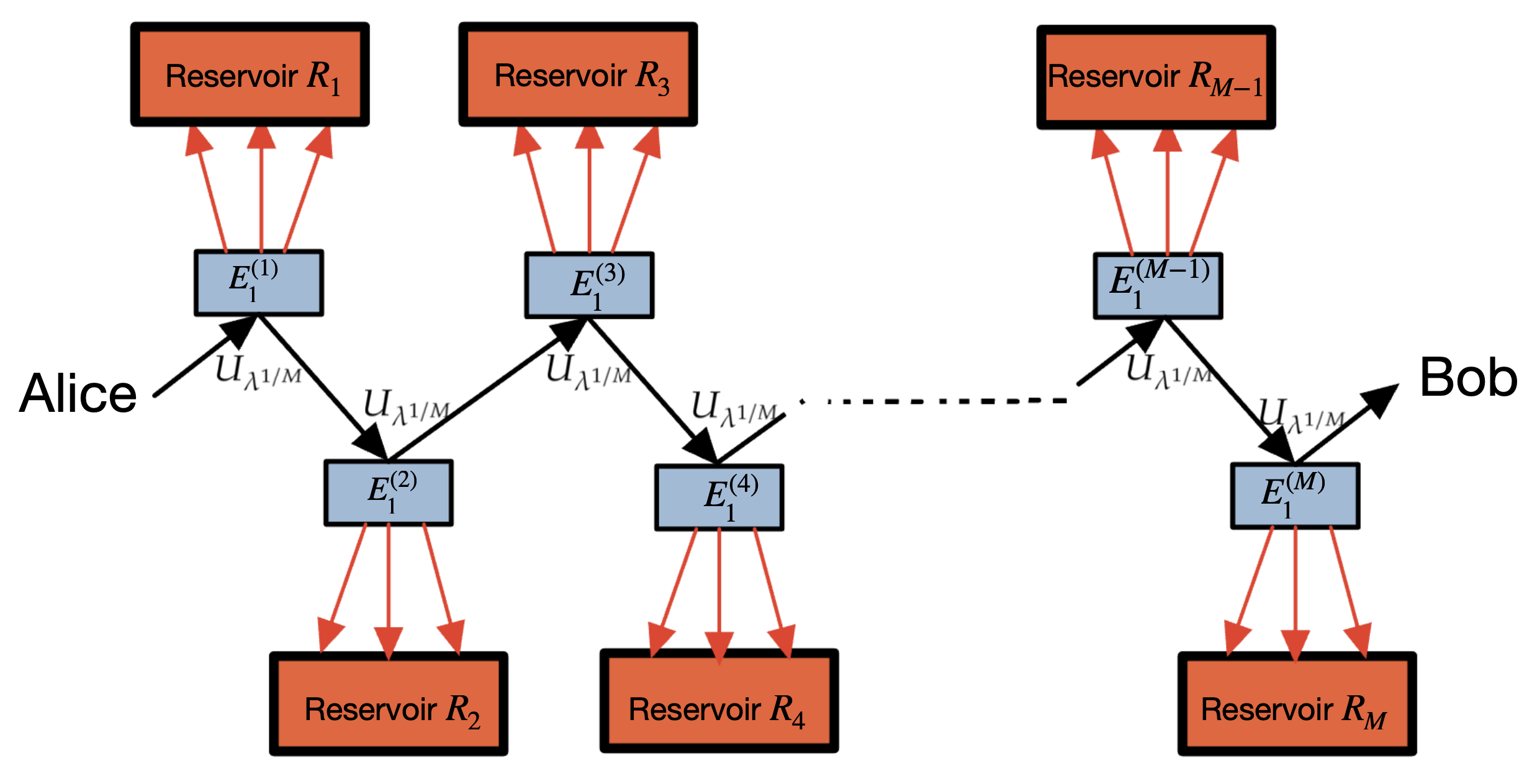
Figure 5: Depiction of our model of optical fibre with memory effects, dubbed "Delocalised Interaction Model" (DIM). As Alice’s input signal travels across the optical fibre, it interacts with each of the $M$ single-mode environments via the beam splitter unitary $U_{\lambda^{1/M}}$. For each $j=1,2,\ldots,M$, the environment $E_{1}^{(j)}$ undergoes a thermalisation process induced by the reservoir $R_{j}$, which attempts to restore the state of $E_{1}^{(j)}$ to its initial thermal state $\tau_{\nu}$. If the time interval between consecutive input signals is much longer than the thermalisation timescale, the memoryless assumption holds, and our model simplifies to that of a thermal attenuator $\mathcal{E}_{\lambda,\nu}$. However, in the opposite regime, where the time interval is shorter than the thermalisation timescale, each environment does not have sufficient time to return to its initial thermal state between consecutive signals. Consequently, in this case, when an input signal interacts with the environments $\{E^{(j)}_{1}\}_{j=1,2,\ldots,M}$, the state of each environment is no longer a thermal state $\tau_{\nu}$, but depends on the previously transmitted input signals, thereby introducing memory effects into the system.

We describe the thermalisation process caused by the reservoir $R_{j}$ on the environment $E_{1}^{(j)}$ as a thermal attenuator $\mathcal{E}_{\mu,\nu}$ with transmissivity $\mu\in[0,1]$ and thermal noise $\nu\geq 0$. The transmissivity $\mu$ serves as a memory parameter that relates to the time interval $\delta t$ between consecutive signals from Alice and the characteristic thermalisation time $t_{E}$. Specifically, we can define $\mu\coloneqq\exp(-\delta t/t_{E})$ as a possible relationship between these quantities.

Let us consider the special case of $\mu=0$ to further enhance our understanding. In this case, the property $\mathcal{E}_{\mu=0,\nu}(\rho)=\tau_{\nu}$ holds for all single-mode states $\rho$. This means that when an input signal interacts with any environment $E_{1}^{(j)}$, the state of $E_{1}^{(j)}$ just before the interaction is a thermal state $\tau_{\nu}$, regardless of the previously sent input signals. As a result, in this case, we can represent each infinitesimal optical fibre as a thermal attenuator $\mathcal{E}_{\lambda^{1/M},\nu}$ with transmissivity $\lambda^{1/M}$. Finally, according to the composition rule (S17), the composition of $M$ thermal attenuators with transmissivity $\lambda^{1/M}$ is equal to a single thermal attenuator with transmissivity $\lambda$.

On the other hand, when $\mu>0$, the environments $\{E_{1}^{(j)}\}_{j=1,2,\ldots,M}$ deviate from the initial thermal state $\tau_{\nu}^{\otimes M}$ at the moment of the interaction with Alice’s signal, and their state becomes dependent on the previously transmitted input signals. This indicates that when $\mu>0$, memory effects come into play. The interaction of each input signal with the environments introduces a memory effect, causing the state of the environments to be influenced by the history of the transmitted signals. Thus, the presence of non-zero $\mu$ leads to the emergence of memory effects in the system.

Now, let us define the quantum channel describing our model of optical fibre with memory effects. In our model, fixed $\lambda\in[0,1]$, $\nu\geq 0$, and $\mu\in[0,1]$, the output state of $n\in\mathds{N}$ uses of the optical fibre corresponds to the output of the $n$-mode quantum channel $\Phi_{\lambda,\mu,\nu}^{(M,n)}$ whose interferometric representation is given in Fig. 6 (see also Fig. 2(c) in the main text), in the strong limit $M\rightarrow\infty$. In the forthcoming Theorem S8 we demonstrate the existence of the following strong limit:

$$\Phi_{\lambda,\mu,\nu}^{(n)}\coloneqq\lim\limits_{M\rightarrow\infty}\Phi_{\lambda,\mu,\nu}^{(M,n)}\qquad\text{(strongly)}\,,$$ (S25)

and we give an explicit expression for it. The family of quantum channels $\{\Phi_{\lambda,\mu,\nu}^{(n)}\}_{n\in\mathds{N}}$ defined in (S25) is a quantum memory channel [12], which completely defines our new model of optical fibre with memory effects, dubbed "Delocalised Interaction Model" (DIM). In the DIM, when Alice transmits an $n$-mode state $\rho^{(n)}\in\mathfrak{S}(L^{2}(\mathbb{R})^{\otimes n})$ through $n$ uses of the optical fibre, Bob receives $n$ signals in the $n$-mode state $\Phi_{\lambda,\mu,\nu}^{(n)}(\rho^{(n)})$.

Figure 6: Depiction of the $n$-mode quantum channel $\Phi_{\lambda,\mu,\nu}^{(M,n)}$, which defines the "Delocalised Interaction Model" (DIM). Here, $M\in\mathds{N}$ is the number of infinitesimal optical fibres, $n\in\mathds{N}$ is the number of uses of the optical fibre, $\lambda$ is the transmissivity of the optical fibre, $\nu$ is the thermal noise, and $\mu$ is the memory parameter. For all $i=1,2,\ldots,n$, the $i$th row of the figure, which consists of $M$ blue beam splitters of transmissivity $\lambda^{1/M}$, represents the $i$th use of the optical fibre. For all $j=1,2,\ldots,M$, the $j$th column of the figure, which consists of $n$ blue splitters of transmissivity $\lambda^{1/M}$ and $n$ yellow beam splitters of transmissivity $\mu$, represents the $j$th infinitesimal optical fibre. The yellow beam splitters, coupling the environments with the thermal state $\tau_{\nu}$, represent the thermalisation process $\mathcal{E}_{\mu,\nu}$. If $\mu=0$ then $\Phi_{\lambda,\mu=0,\nu}^{(M,n)}=\mathcal{E}_{\lambda,\nu}^{\otimes n}$, meaning that the memoryless scenario is recovered. In the Heisenberg representation, $\Phi_{\lambda,\mu,\nu}^{(M,n)}$ maps the annihilation operator $a_{i}$ (depicted on the left) of the $i$th input signal into the annihilation operators $a_{i,M}$ (depicted on the right) of the $i$th output signal for all $i=1,2,\ldots,n$. Our model of optical fibre with memory effects coincides with the strong limit $\Phi_{\lambda,\mu,\nu}^{(n)}=\lim\limits_{M\rightarrow\infty}\Phi_{\lambda,\mu,\nu}^{(M,n)}$.

Theorem S8.

Let $\lambda\in[0,1]$, $\nu\geq 0$, $\mu\in[0,1]$, and $n\in\mathds{N}$. The strong limit $\Phi_{\lambda,\mu,\nu}^{(n)}\coloneqq\lim\limits_{M\rightarrow\infty}\Phi_{\lambda,\mu,\nu}^{(M,n)}$ exists and it reads

$$\Phi_{\lambda,\mu,\nu}^{(n)}=\mathcal{U}_{O_{2}^{T}}\circ\left(\bigotimes_{i=1}^{n}\mathcal{E}_{\eta_{i}^{(n,\lambda,\mu)},\nu}\right)\circ\mathcal{U}_{O_{1}}\,,$$ (S26)

i.e.

$$\lim\limits_{M\rightarrow\infty}\left\|\Phi_{\lambda,\mu,\nu}^{(M,n)}(\rho^{(n)})-\mathcal{U}_{O_{2}^{T}}\circ\left(\bigotimes_{i=1}^{n}\mathcal{E}_{\eta_{i}^{(n,\lambda,\mu)},\nu}\right)\circ\mathcal{U}_{O_{1}}(\rho^{(n)})\right\|_{1}=0\qquad\forall\,\rho^{(n)}\in\mathfrak{S}(L^{2}(\mathbb{R}^{\otimes n}))\,.$$ (S27)

Here,

• $\mathcal{U}_{O_{2}^{T}}$ and $\mathcal{U}_{O_{1}}$ are passive unitary operators on $L^{2}(\mathbb{R}^{\otimes n})$ (see Remark 1 for the definition of passive unitary operators) associated with the orthogonal matrices $O_{2}^{T}$ and $O_{1}$ (defined below), respectively.

• The transmissivities $\{\eta_{i}^{(n,\lambda,\mu)}\}_{i=1,2,\ldots,n}$ of the $n$-mode thermal attenuator in (S26) and the $n\times n$ orthogonal matrices $O_{2}^{T}$ and $O_{1}$ are defined by means of the singular value decomposition of the $n\times n$ real matrix $\bar{A}^{(n,\lambda,\mu)}$ (defined below):

  $$\bar{A}^{(n,\lambda,\mu)} =O_{2}^{T}DO_{1}\,,$$ (S28)

  where $D\coloneqq\text{diag}(\sqrt{\eta_{1}^{(n,\lambda,\mu)}},\sqrt{\eta_{2}^{(n,\lambda,\mu)}},\ldots,\sqrt{\eta_{n}^{(n,\lambda,\mu)}})$ is an $n\times n$ positive diagonal matrix with

  $$1\geq\eta_{n}^{(n,\lambda,\mu)}\geq\eta_{n-1}^{(n,\lambda,\mu)}\geq\ldots\geq\eta_{1}^{(n,\lambda,\mu)}\geq 0\,.$$ (S29)

• For each $i,k\in\{1,2,\ldots,n\}$, the $(i,k)$ element of the $n\times n$ real matrix $\bar{A}^{(n,\lambda,\mu)}$ is defined as

  $$\bar{A}^{(n,\lambda,\mu)}_{i,k}=\Theta(i-k)\,\sqrt{\lambda}\mu^{\frac{i-k}{2}}L_{i-k}^{(-1)}(-\ln\lambda)\,.$$ (S30)

  where $\Theta:\mathbb{R}\to\mathbb{R}$ is the Heaviside Theta function defined as

  $$\Theta(x)\coloneqq\begin{cases}1,&\text{if $x\geq 0$,}\\ 0,&\text{otherwise.}\end{cases}$$ (S31)

  and where $\{L_{m}^{(-1)}\}_{m\in\mathds{N}}$ are the generalised Laguerre polynomials defined as

  $$L_{m}^{(-1)}(x) \coloneqq\sum_{l=1}^{m}\binom{m-1}{l-1}\frac{(-x)^{l}}{l!}\qquad\forall\,m\in\mathbb{N}^{+}\,,$$ (S32)

  $$L_{0}^{(-1)}(x) \coloneqq 1\,,$$

  for all $x\in\mathbb{R}$.

(S27) establishes that the quantum memory channel $\{\Phi_{\lambda,\mu,\nu}^{(n)}\}_{n\in\mathds{N}}$ is unitarily equivalent to $\{\bigotimes_{i=1}^{n}\mathcal{E}_{\eta_{i}^{(n,\lambda,\mu)},\nu}\}_{n\in\mathds{N}}$. In particular, their (energy-constrained and unconstrained) capacities coincide.

Before presenting the proof of Theorem S8, let us understand its meaning. Suppose Alice prepares an $n$-signal state $\rho^{(n)}\in\mathfrak{S}(L^{2}(\mathbb{R})^{\otimes n})$, applies the passive transformation $\mathcal{U}_{O_{1}^{T}}$, and then sends each of the $n$ signals through the optical fibre. After receiving the signals, Bob applies the passive transformation $\mathcal{U}_{O_{2}}$. Consequently, Bob receives the state $\mathcal{U}_{O_{2}}\circ\Phi_{\lambda,\mu,\nu}^{(n)}\circ\mathcal{U}_{O_{1}^{T}}(\rho^{(n)})$ which can be expresses as

$$\mathcal{U}_{O_{2}}\circ\Phi_{\lambda,\mu,\nu}^{(n)}\circ\mathcal{U}_{O_{1}^{T}}(\rho^{(n)})=\bigotimes_{i=1}^{n}\mathcal{E}_{\eta_{i}^{(n,\lambda,\mu)},\nu}(\rho^{(n)})\,,$$ (S33)

thanks to Theorem S8. Therefore, by employing appropriate encoding and decoding passive unitary transformations, Alice and Bob can effectively communicate via

$$\left\{\bigotimes_{i=1}^{n}\mathcal{E}_{\eta_{i}^{(n,\lambda,\mu)},\nu}\right\}_{n\in\mathbb{N}}\,,$$ (S34)

instead of via $\{\Phi_{\lambda,\mu,\nu}^{(n)}\}_{n\in\mathbb{N}}$. To summarise, the quantum memory channel $\Phi_{\lambda,\mu,\nu}^{(n)}$, which models $n$ uses of the optical fibre, is unitarily equivalent to a tensor product of $n$ distinct thermal attenuators. These attenuators have the same thermal noise $\nu$ but differ in their transmissivities. This equivalence allows us to understand the behaviour of the quantum memory channel in terms of individual thermal attenuators operating on each signal independently. The transmissivities $\{\eta_{i}^{(n,\lambda,\mu)}\}_{i=1,2,\ldots,n}$ can be calculated via the singular value decomposition of the matrix reported in (S30). Notably, each element of this matrix depends solely on the difference between the row and column indices, making it a Toeplitz matrix. In Section IV we will review important properties of Toeplitz matrices. Fortunately, these matrices allow for the calculation of the asymptotic distribution of their singular values as the dimension approaches infinity. Leveraging this observation, we will be able to analytically determine the transmissivities $\{\eta_{i}^{(n,\lambda,\mu)}\}_{i=1,2,\ldots,n}$ as the number of uses of the optical fibre, $n$, approaches infinity.

Now, we are ready to proceed with the proof of Theorem S8, which follows and generalises the methods used in [16, 17, 18]

Proof of Theorem S8.

In this proof, we will adopt the notation introduced in Fig. 6 and in Fig. 2(c) in the main text. Specifically, $n\in\mathds{N}$ represents the number of uses of the optical fibre, while $M\in\mathds{N}$ represents the number of infinitesimal optical fibres. Moreover, for each $i=1,2,\ldots,n$ the annihilation operator associated with the $i$th input signal is denoted as $a_{i}$, and for each $j=1,2,\ldots,M$ the annihilation operator associated with the $j$th single-mode environment $E_{1}^{(j)}$ is denoted as $b_{1}^{(j)}$. In addition, as shown in Fig. 2(c) in the main text, for each $i=2,3,\ldots n$ and $j=1,2,\ldots,M$ we denote as $E_{i}^{(j)}$ the single-mode environment associated with the thermal attenuator $\mathcal{E}_{\mu,\nu}$ that represents the thermalisation process acting on the $j$th environment $E_{1}^{(j)}$ right before the $i$th use of the fibre. As shown in Fig. 6, the annihilation operator of the environment $E_{i}^{(j)}$ is denoted as $b_{i}^{(j)}$.

Let $U_{\lambda,\mu}^{(n,M)}$ be the unitary operator implementing the physical representation of $\Phi_{\lambda,\mu,\nu}^{(M,n)}$ in Fig. 6:

$$\Phi_{\lambda,\mu,\nu}^{(M,n)}(\rho^{(n)})=\operatorname{Tr}_{E}\left[U_{\lambda,\mu}^{(n,M)}\left(\rho^{(n)}\otimes\tau_{\nu}^{\otimes nM}\right){U_{\lambda,\mu}^{(n,M)}}^{\dagger}\right]\qquad\,\forall\,\rho^{(n)}\in\mathfrak{S}(L^{2}(\mathbb{R})^{\otimes n})\,,$$ (S35)

where $\operatorname{Tr}_{E}$ denotes the partial trace over all the environment systems ($E_{i}^{(j)}$ for all $i=1,2,\ldots,n$ and all $j=1,2,\ldots,M$). In addition, as shown in Fig. 6, for each $i=1,2,\ldots,n$ let $a_{i,M}\coloneqq{U_{\lambda,\mu}^{(n,M)}}^{\dagger}a_{i}U_{\lambda,\mu}^{(n,M)}$ be the output of the $i$th annihilation operator in Heisenberg representation.

Since the unitary $U_{\lambda,\mu}^{(n,M)}$ is composed of only beam splitters (see Fig. 6), (S11) implies that for all $i=1,2,\ldots,M$ the output annihilation operator $a_{i,M}$ can be written as

$$a_{i,M}=\sum_{h=1}^{n}A^{(M,n,\lambda,\mu)}_{i,h}\,a_{h}+\sum_{l=1}^{M}\sum_{h=1}^{n}E^{(M,n,\lambda,\mu)}_{l,i,h}\,b_{h}^{(l)}\,,$$ (S36)

where $A^{(M,n,\lambda,\mu)}_{i,h}$ and $E^{(M,n,\lambda,\mu)}_{l,i,h}$ are suitable real numbers such that

$$[a_{i,M},(a_{j,M})^{\dagger}]=\delta_{i,j}\mathbb{1}\,.$$ (S37)

Note that (S36) holds because the transformations in (S11) maps annihilation operators into annihilation operators (without introducing any creation operator). By defining the following vectors of annihilation operators

$$\mathbf{a} \coloneqq(a_{1},\,a_{2},\ldots,\,a_{n})^{T}\,,$$ (S38)

$$\mathbf{a_{M}} \coloneqq(a_{1,M},\,a_{2,M},\ldots,\,a_{n,M})^{T}\,,$$

$$\mathbf{b} \coloneqq(b_{1}^{(1)},\,b_{1}^{(2)},\ldots,\,b_{1}^{(M)},\,b_{2}^{(1)},\,b_{2}^{(2)},\ldots,\,b_{2}^{(M)},\ldots,\,b_{n}^{(1)},\,b_{n}^{(2)},\ldots,\,b_{n}^{(M)})^{T}\,,$$

one can rewrite (S36) as

$$\mathbf{a_{M}}=A^{(M,n,\lambda,\mu)}\mathbf{a}+E^{(M,n,\lambda,\mu)}\mathbf{b}\,,$$ (S39)

where $A^{(M,n,\lambda,\mu)}$ is an $n\times n$ real matrix and $E^{(M,n,\lambda,\mu)}$ is an $n\times nM$ real matrix which satisfy

$$A^{(M,n,\lambda,\mu)}{A^{(M,n,\lambda,\mu)}}^{T}+E^{(M,n,\lambda,\mu)}{E^{(M,n,\lambda,\mu)}}^{T}=\mathbb{1}_{n\times n}\,,$$ (S40)

thanks to (S37). Here, $\mathbb{1}_{n\times n}$ denotes the $n\times n$ identity matrix.

Below we will show that the limit of the matrix element $\lim\limits_{M\rightarrow\infty}A_{i,h}^{(M,n,\lambda,\mu)}$ does exist and it is given by (S30) for all $i,h=1,2,\ldots n$. Hence, we can define the matrix $\bar{A}^{(n,\lambda,\mu)}$ whose $(i,h)$ element is equal to

$$\bar{A}_{i,h}^{(n,\lambda,\mu)}\coloneqq\lim\limits_{M\rightarrow\infty}A_{i,h}^{(M,n,\lambda,\mu)}\,.$$ (S41)

Now, we will demonstrate the validity of (S27). For this purpose, let $\rho^{(n)}\in\mathfrak{S}(L^{2}(\mathbb{R})^{\otimes n})$ be an $n$-mode input state. The characteristic function of $\Phi_{\lambda,\mu,\nu}^{(M,n)}(\rho^{(n)})$ can be calculated as

$$\chi_{\Phi_{\lambda,\mu,\nu}^{(M,n)}(\rho^{(n)})}(\mathbf{z}) \coloneqq\operatorname{Tr}\left[\Phi_{\lambda,\mu,\nu}^{(M,n)}(\rho^{(n)})\,e^{\mathbf{a}^{\dagger}\mathbf{z}-\mathbf{z}^{\dagger}\mathbf{a}}\right]$$ (S42)

$$\stackrel{{\scriptstyle\mathclap{\scriptsize\mbox{(i)}}}}{{=}}\chi_{\rho^{(n)}}\left({A^{(M,n,\lambda,\mu)}}^{T}\mathbf{z}\right)\chi_{\tau_{\nu}^{\otimes nM}}\left({E^{(M,n,\lambda,\mu)}}^{T}\mathbf{z}\right)$$

$$\stackrel{{\scriptstyle\mathclap{\scriptsize\mbox{(ii)}}}}{{=}}\chi_{\rho^{(n)}}\left({A^{(M,n,\lambda,\mu)}}^{T}\mathbf{z}\right)e^{-(\nu+\frac{1}{2})\mathbf{z}^{\dagger}E^{(M,n,\lambda,\mu)}{E^{(M,n,\lambda,\mu)}}^{T}\mathbf{z}}$$

$$\stackrel{{\scriptstyle\mathclap{\scriptsize\mbox{(iii)}}}}{{=}}\chi_{\rho^{(n)}}\left({A^{(M,n,\lambda,\mu)}}^{T}\mathbf{z}\right)e^{-(\nu+\frac{1}{2})\mathbf{z}^{\dagger}(\mathbb{1}_{n\times n}-A^{(M,n,\lambda,\mu)}{A^{(M,n,\lambda,\mu)}}^{T})\mathbf{z}}\qquad\forall\,\mathbf{z}\in\mathbb{C}^{n}\,,$$

where: in (i) we exploited (S35) and (S39); in (ii) we used the expression in (S15) of the characteristic function of the thermal state $\tau_{\nu}$; in (iii) we just exploited (S40). Since $\lim\limits_{M\rightarrow\infty}A^{(M,n,\lambda,\mu)}\mathbf{z}=\bar{A}^{(n,\lambda,\mu)}\mathbf{z}$ (thanks to (S41)) and since every characteristic function is continuous [24, 54], it holds that

$$\lim\limits_{M\rightarrow\infty}\chi_{\Phi_{\lambda,\mu,\nu}^{(M,n)}(\rho^{(n)})}(\mathbf{z})=\chi_{\rho^{(n)}}\left(\bar{A}^{(n,\lambda,\mu)^{T}}\mathbf{z}\right)e^{-(\nu+\frac{1}{2})\mathbf{z}^{\dagger}(\mathbb{1}_{n\times n}-\bar{A}^{(n,\lambda,\mu)}\bar{A}^{(n,\lambda,\mu)^{T}})\mathbf{z}}\,.$$ (S43)

By applying the singular value decomposition, $\bar{A}^{(n,\lambda,\mu)}$ can be written as

$$\bar{A}^{(n,\lambda,\mu)} =O_{2}^{T}DO_{1}\,,$$ (S44)

where $O_{1}$ and $O_{2}$ are $n\times n$ real orthogonal matrices, $D=\text{diag}(s_{1}^{(n,\lambda,\mu)},s_{2}^{(n,\lambda,\mu)},\ldots,s_{n}^{(n,\lambda,\mu)})$ is an $n\times n$ positive diagonal matrix with

$$1\geq s_{n}^{(n,\lambda,\mu)}\geq s_{n-1}^{(n,\lambda,\mu)}\geq\ldots\geq s_{1}^{(n,\lambda,\mu)}\geq 0\,,$$ (S45)

where the fact that $s_{n}^{(n,\lambda,\mu)}\leq 1$ follows from (S40). Let us define for all $i=1,2,\ldots,n$ the $i$th transmissivity $\eta_{i}^{(n,\lambda,\mu)}$ as the square of the $i$th diagonal element of $D$, i.e.

$$\eta_{i}^{(n,\lambda,\mu)}\coloneqq(s_{i}^{(n,\lambda,\mu)})^{2}\,.$$ (S46)

Note that $\eta_{i}^{(n,\lambda,\mu)}$ is a proper transmissivity because $0\leq(s_{i}^{(n,\lambda,\mu)})^{2}\leq 1$. In addition, for all $\mathbf{z}\in\mathbb{C}^{n}$ it holds that

$$\lim\limits_{M\rightarrow\infty}\chi_{\Phi_{\lambda,\mu,\nu}^{(M,n)}(\rho^{(n)})}(\mathbf{z}) \stackrel{{\scriptstyle\mathclap{\scriptsize\mbox{(i)}}}}{{=}}\chi_{\rho^{(n)}}\left(O_{1}^{T}DO_{2}\mathbf{z}\right)e^{-(\nu+\frac{1}{2})\mathbf{z}^{\dagger}(\mathbb{1}_{n\times n}-O_{2}^{T}D^{2}O_{2})\mathbf{z}}$$ (S47)

$$\stackrel{{\scriptstyle\mathclap{\scriptsize\mbox{(ii)}}}}{{=}}\chi_{\mathcal{U}_{O_{1}}(\rho^{(n)})}\left(DO_{2}\mathbf{z}\right)e^{-(\nu+\frac{1}{2})\mathbf{z}^{\dagger}O_{2}^{T}(\mathbb{1}_{n\times n}-D^{2})O_{2}\mathbf{z}}$$

$$\stackrel{{\scriptstyle\mathclap{\scriptsize\mbox{(iii)}}}}{{=}}\chi_{\mathcal{U}_{O_{1}}(\rho^{(n)})}\left(DO_{2}\mathbf{z}\right)\chi_{\tau_{\nu}^{\otimes n}}(\sqrt{\mathbb{1}_{n\times n}-D^{2}}O_{2}\mathbf{z})$$

$$\stackrel{{\scriptstyle\mathclap{\scriptsize\mbox{(iv)}}}}{{=}}\chi_{(\bigotimes_{i=1}^{n}\mathcal{E}_{\eta_{i}^{(n,\lambda,\mu)},\nu})\circ\mathcal{U}_{O_{1}}(\rho^{(n)})}\left(O_{2}\mathbf{z}\right)$$

$$\stackrel{{\scriptstyle\mathclap{\scriptsize\mbox{(v)}}}}{{=}}\chi_{\mathcal{U}_{O_{2}^{T}}\circ\left(\bigotimes_{i=1}^{n}\mathcal{E}_{\eta_{i}^{(n,\lambda,\mu)},\nu}\right)\circ\mathcal{U}_{O_{1}}(\rho^{(n)})}\left(\mathbf{z}\right)\,\,,$$

where: in (i) we used (S43) and (S44); in (ii) we exploited Remark (1); (iii) is a consequence of the expression in (S15) of the characteristic function of the thermal state $\tau_{\nu}$; (iv) comes from the expression in (S16) of the characteristic function of the output state of the thermal attenuator; in (v) we exploited again Remark (1). Hence, (S47) establishes that the characteristic function of ${\Phi_{\lambda,\mu,\nu}^{(M,n)}(\rho^{(n)})}_{M\in\mathds{N}}$ converges pointwise for $M\rightarrow\infty$ to the characteristic function $\mathcal{U}_{O_{2}^{T}}\circ\left(\bigotimes_{i=1}^{n}\mathcal{E}_{\eta_{i}^{(n,\lambda,\mu)},\nu}\right)\circ\mathcal{U}_{O_{1}}(\rho^{(n)})$. Consequently, Lemma (S7) implies that

$$\lim\limits_{M\rightarrow\infty}\left\|\Phi_{\lambda,\mu,\nu}^{(M,n)}(\rho^{(n)})-\mathcal{U}_{O_{2}^{T}}\circ\left(\bigotimes_{i=1}^{n}\mathcal{E}_{\eta_{i}^{(n,\lambda,\mu)},\nu}\right)\circ\mathcal{U}_{O_{1}}(\rho^{(n)})\right\|_{1}=0\,,$$ (S48)

i.e. we have proved (S27).

Now, we only need to show that the limit $\lim\limits_{M\rightarrow\infty}A_{i,h}^{(M,n,\lambda,\mu)}$ does exist and it is given by (S30) for all $i,h=1,2,\ldots n$. To proceed, we begin by calculating the elements of the matrix $A^{(M,n,\lambda,\mu)}$ defined in (S39). Our goal is thus to express $a_{i,M}$ in terms of $a_{1},a_{2},\ldots,a_{n}$.

In the following derivation, $m_{i,j}$ and $a_{i,j}$ denote the annihilation operators in Heisenberg representation introduced in Fig. 6. Specifically, $m_{i,j}$ denotes the Heisenberg evolution of the annihilation operator $b_{1}^{(j)}$ right before the $(i+1)$th use of the fibre. Moreover, $a_{i,j}$ denotes the Heisenberg evolution of the annihilation operator $a_{i}$ of the $i$th input signal right after its transmission through the first $j$ beam splitters of transmissivity $\lambda^{1/M}$. Additionally, we use the notations $a_{i,0}\coloneqq a_{i}$ and $m_{0,i}\coloneqq b^{(i)}_{1}$. By exploiting (S11), one deduces that for all $i=1,2,\ldots,n$ and all $j=1,2,\ldots,M$ it holds that

$$a_{i,j} =\sqrt{\lambda^{1/M}}\,a_{i,j-1}+\sqrt{1-\lambda^{1/M}}\,m_{i-1,j}\,,$$ (S49)

$$m_{i,j} =-\sqrt{1-\mu}\,b_{i+1}^{(j)}+\sqrt{\mu\lambda^{1/M}}\,m_{i-1,j}-\sqrt{\mu(1-\lambda^{1/M})}\,a_{i,j-1}\,.$$

Consequently, $a_{i,M}$ can be expressed as a linear combination of the annihilation operators $\{a_{i}\}_{i}$ and $\{b_{i}^{(j)}\}_{i,j}$. In order to calculate the matrix $A^{(M,n,\lambda,\mu)}$, we only need to calculate the coefficients of $\{a_{i}\}_{i}$ in the expression of $a_{i,M}$, while we do not need to calculate the coefficients of $\{b_{i}^{(j)}\}_{i,j}$. Hence, we introduce the relation $A\simeq B$ between operators as follows:

$$A\simeq B\quad\Longleftrightarrow\quad A=B+\text{linear combination of $\{b_{i}^{(j)}\}_{i,j}$. }$$ (S50)

Note that (S49) implies that for all $i=1,2,\ldots,n$ and all $j=1,2,\ldots,M$ it holds that

$$a_{i,j} =\sqrt{\lambda^{j/M}}\,a_{i}+\sqrt{1-\lambda^{1/M}}\sum_{l=1}^{j}\lambda^{\frac{j-l}{2M}}\,m_{i-1,l}$$ (S51)

and

$$m_{i,j} \simeq\sqrt{\mu\lambda^{1/M}}m_{i-1,j}-\sqrt{\mu(1-\lambda^{1/M})}a_{i,j-1}\,$$ (S52)

$$=\sqrt{\mu\lambda^{1/M}}m_{i-1,j}-\sqrt{\mu(1-\lambda^{1/M})\lambda^{(j-1)/M}}a_{i}-\sqrt{\mu}(1-\lambda^{1/M})\sum_{l=1}^{j-1}\lambda^{\frac{j-1-l}{2M}}m_{i-1,l}\,.$$

From (S51) we deduce that in order to express $a_{i,M}$ in terms of $\{a_{i}\}_{i}$, we now only need to express $\{m_{i,l}\}_{i,l}$ in terms of $\{a_{i}\}_{i}$ by solving the recurrence relation in (S52). One can show that the latter implies that for all $i=1,2,\ldots,n$ and all $j=2,3\ldots,M$ it holds that

$$m_{i,1} \simeq-\sqrt{\mu(1-\lambda^{1/M})}\sum_{l=1}^{i}\left({\mu\lambda^{1/M}}\right)^{\frac{i-l}{2}}\,a_{l}\,,$$ (S53)

$$m_{i,j} \simeq\sqrt{\mu\lambda^{1/M}}\,m_{i-1,j}-\sqrt{\mu}\,m_{i-1,j-1}+\sqrt{\lambda^{1/M}}\,m_{i,j-1}\,.$$

As a consequence of this, substituting terms $m_{l,j}$ with $l\leq i$, through repeated application of the second equality, and finally dropping the term $m_{0,j}$, one can show that

$$m_{i,j}\simeq\lambda^{\frac{1}{2M}}\,m_{i,j-1}+(\lambda^{\frac{1}{2M}}-\lambda^{-\frac{1}{2M}})\sum_{l=1}^{i-1}(\mu\lambda^{1/M})^{\frac{i-l}{2}}\,m_{l,j-1}$$ (S54)

We stress that, here and in the following, summations are zero whenever the lower extreme is strictly larger than the upper extreme. By defining $\tilde{m}_{i,j}\coloneqq\lambda^{-\frac{j}{2M}}(\mu\lambda^{1/M})^{-\frac{i}{2}}\,m_{i,j}$, the recurrence relation in (S54) can be rewritten as

$$\tilde{m}_{i,j} \simeq\tilde{m}_{i,j-1}+(1-\lambda^{-\frac{1}{M}})\sum_{l=1}^{i-1}\tilde{m}_{l,j-1}\,.$$ (S55)

In order to solve this, let us introduce the following notation:

$$\mathcal{F}_{i,n}\left(\{\tilde{m}_{\cdot,1}\}\right)\coloneqq\sum_{i_{n}=1}^{i-1}\sum_{i_{n-1}=1}^{i_{n}-1}\dots\sum_{i_{1}=1}^{i_{2}-1}\tilde{m}_{i_{1},1}\,.$$ (S56)

By noting that the cardinality of the set $\{(i_{2},\ldots,i_{n})\in\mathbb{N}^{n-1}\,:\,i>i_{n}>i_{n-1}>\ldots>i_{2}>d\}$ is $\binom{i-d-1}{n-1}$, we deduce that

$$\mathcal{F}_{i,n}\left(\{\tilde{m}_{\cdot,1}\}\right)=\sum_{d=1}^{i-n}\binom{i-d-1}{n-1}\tilde{m}_{d,1}\,.$$ (S57)

In addition, note that

$$\mathcal{F}_{i,n}\left(\{\tilde{m}_{\cdot,1}\}\right) =0\qquad\text{if }i\leq n\,,$$ (S58)

and

$$\sum_{l=1}^{i-1}\mathcal{F}_{l,n}\left(\{\tilde{m}_{\cdot,1}\}\right) =\mathcal{F}_{i,n+1}\left(\{\tilde{m}_{\cdot,1}\}\right)\,.$$ (S59)

As a consequence, by exploiting (S55), one can show by induction that for all $i=1,2,\ldots,n$ and all $j=1,2,\ldots,M$ it holds that

$$\tilde{m}_{i,j}\simeq\tilde{m}_{i,1}+\sum_{l=1}^{j-1}\binom{j-1}{l}(1-\lambda^{-1/M})^{l}\mathcal{F}_{i,l}\left(\{\tilde{m}_{\cdot,1}\}\right)\,,$$ (S60)

and from this one can obtain

$$m_{i,j}\simeq\sum_{k=1}^{i}\mu^{\frac{i-k+1}{2}}\lambda^{\frac{j+i-k+1}{2M}}\sqrt{1-\lambda^{1/M}}\left[\sum_{l=0}^{\min(i-k,j-1)}\binom{j-1}{l}\binom{i-k}{l}(1-\lambda^{-1/M})^{l}\right]a_{k}$$ (S61)

Consequently, (S51) implies that

$$a_{i,M} =\sqrt{\lambda}a_{i}+\sqrt{1-\lambda^{1/M}}\sum_{j=1}^{M}\lambda^{\frac{M-j}{2M}}m_{i-1,j}$$ (S62)

$$\simeq\sum_{k=1}^{n}\left[\sqrt{\lambda}\delta_{i,k}-\Theta(i-k-1)\,\mu^{\frac{i-k}{2}}\lambda^{\frac{M+i-k}{2M}}(1-\lambda^{1/M})\sum_{j=1}^{M}\sum_{l=0}^{\min(i-k-1,j-1)}\binom{j-1}{l}\binom{i-k-1}{l}(1-\lambda^{-1/M})^{l}\right]a_{k},$$

where we have introduced the Heaviside function $\Theta(x)$ defined as $\Theta(x)=1$ if $x\geq 0$, and $\Theta(x)=0$ if $x<0$. Hence, we deduce that for all $i,k\in\{1,2,\ldots,n\}$ the $(i,k)$ matrix element of $A^{(M,n,\lambda,\mu)}$ is

$$A^{(M,n,\lambda,\mu)}_{i,k} =\sqrt{\lambda}\delta_{i,k}-\Theta(i-k-1)\,\mu^{\frac{i-k}{2}}\lambda^{\frac{M+i-k}{2M}}(1-\lambda^{1/M})\sum_{j=1}^{M}\sum_{l=0}^{\min(i-k-1,j-1)}\binom{j-1}{l}\binom{i-k-1}{l}(1-\lambda^{-1/M})^{l}.$$ (S63)

The sum over $j$ can be split in two parts, obtaining

$$(1-\lambda^{1/M})\sum_{j=1}^{M}\sum_{l=0}^{\min(i-k-1,j-1)}\binom{j-1}{l}\binom{i-k-1}{l}(1-\lambda^{-1/M})^{l}$$ (S64)

$$=(1-\lambda^{1/M})\sum_{j=1}^{i-k}\sum_{l=0}^{j-1}\binom{j-1}{l}\binom{i-k-1}{l}(1-\lambda^{-1/M})^{l}+(1-\lambda^{1/M})\sum_{j=i-k+1}^{M}\sum_{l=0}^{i-k-1}\binom{j-1}{l}\binom{i-k-1}{l}(1-\lambda^{-1/M})^{l}.$$

The limit for $M\rightarrow\infty$ of the first piece is zero, while for the second we use that

$$\lim_{M\rightarrow\infty}(1-\lambda^{1/M})\sum_{j=i-k+1}^{M}\binom{j-1}{l}(1-\lambda^{-1/M})^{l}=-\frac{(\ln\lambda)^{l+1}}{(l+1)!}$$ (S65)

to obtain

$$\bar{A}^{(n,\lambda,\mu)}_{i,k}\coloneqq\lim\limits_{M\rightarrow\infty}A^{(M,n,\lambda,\mu)}_{i,k}=\sqrt{\lambda}\left[\delta_{i,k}+\Theta(i-k-1)\,\mu^{\frac{i-k}{2}}\sum_{l=1}^{i-k}\binom{i-k-1}{l-1}\frac{(\ln\lambda)^{l}}{l!}\right]\,.$$ (S66)

By defining the generalised Laguerre polynomial $L_{m}^{(-1)}(x)\coloneqq\sum_{l=1}^{m}\binom{m-1}{l-1}\frac{(-x)^{l}}{l!}$ for all $x\in\mathbb{R}$ and $m\in\mathbb{N}^{+}$ and $L_{0}^{(-1)}(x)\coloneqq 1$, for all $i,k\in\{1,2,\ldots,n\}$ the $(i,k)$ matrix element of $\bar{A}^{(n,\lambda,\mu)}$ in (S66) can be rewritten as

$$\bar{A}^{(n,\lambda,\mu)}_{i,k}=\Theta(i-k)\,\sqrt{\lambda}\mu^{\frac{i-k}{2}}L_{i-k}^{(-1)}(-\ln\lambda)\,.$$ (S67)

∎

III Problems of the "Localised" interaction model solved by the "Delocalised" one

Memory effects in optical fibres have been studied in [16, 17, 18, 11, 10]. As explained in the main text, the model examined in [16, 17, 18, 11, 10] corresponds to a specific case of the DIM we have presented here, specifically the case in which we set $M=1$ (see Section II for the meaning of $M$). This corresponds to the configuration depicted in Fig.2(b) in the main text, where the interaction between the signal and the fibre is localised. For this reason, in the main text we dubbed the model analysed in [16, 17, 18, 11, 10] as "Localised Interaction Model" (LIM). The memory quantum channel characterising the LIM is $\{\Phi_{\lambda,\mu,\nu}^{(1,n)}\}_{n\in\mathds{N}}$ (see Section II for its definition).

However, it is important to note that the LIM is not realistic because it fails to satisfy the following two essential properties that any "reasonable" model of an optical fibre should possess:

• Property 1: When the transmissivity $\lambda$ is exactly equal to zero, no information can be transmitted;

• Property 2: The model is consistent under concatenation of optical fibres. In other words, the concatenation of $k$ optical fibres, each with transmissivity $\lambda_{1},\lambda_{2},\ldots,\lambda_{k}$ and identical thermal noise $\nu$, results in another optical fibre with a transmissivity equal to the product of the individual transmissivities $\lambda_{1}\lambda_{2}\ldots\lambda_{k}$, and with the same thermal noise $\nu$.

Remark 2.

The LIM, which is characterised by the quantum memory channel $\{\Phi_{\lambda,\mu,\nu}^{(1,n)}\}_{n\in\mathds{N}}$, fails to satisfy Property 1.

Proof.

The LIM is associated with the channel $\{\Phi_{\lambda,\mu,\nu}^{(1,n)}\}_{n\in\mathds{N}}$ that transmits information even if $\lambda$ is exactly zero. Indeed, for $\lambda=0$ the channel $\Phi_{0,\mu,\nu}^{(1,n)}$ can be expressed in terms of the quantum shift channel of order $1$, the thermal attenuator $\mathcal{E}_{\mu,\nu}$, and the unitary phase space inversion operation $\mathcal{V}(\cdot)\coloneqq(-1)^{a^{\dagger}a}\cdot(-1)^{a^{\dagger}a}$. Specifically, if the state of the $i$th input signal is $\rho$, then the state of the $(i+1)$th output signal is $\mathcal{V}\circ\mathcal{E}_{\mu,\nu}(\rho)$, which is not constant with respect to $\rho$ for $\mu>0$. ∎

In particular, from the above proof we conclude that the LIM would lead to the paradoxical result that an optical fibre with zero transmissivity and a memory parameter $\mu>0$ is equivalent to a memoryless optical fibre with transmissivity $\mu>0$ with a certain time-delay $\delta t$ (e.g. $\delta t$ can be determined in terms of $\mu$ by $\mu=\exp(-\delta t/t_{E})$), provided the output of the first signal is discarded.

Furthermore, the DIM with a finite value of $M$ is also unrealistic because it fails to satisfy Property 1, as we now demonstrate.

Remark 3.

The DIM with a finite value of $M$, which is characterised by the quantum memory channel $\{\Phi_{\lambda,\mu,\nu}^{(M,n)}\}_{n\in\mathds{N}}$, does not satisfy Property 1.

Proof.

The model with a finite value of $M$ is associated with the channel $\{\Phi_{\lambda,\mu,\nu}^{(M,n)}\}_{n\in\mathds{N}}$ that transmits information even if $\lambda$ is exactly zero. Indeed, for $\lambda=0$ the channel $\Phi_{0,\mu,\nu}^{(M,n)}$ can be expressed in terms of the quantum shift channel of order $M$, the thermal attenuator $\mathcal{E}_{\mu,\nu}$, and the unitary phase space inversion operation $\mathcal{V}^{M\!\!\mod 2}$. Specifically, if the state of the $i$th input signal is $\rho$, then the state of the $(i+M)$th output signal is $\mathcal{V}^{M\!\!\mod 2}\circ\mathcal{E}_{\mu,\nu}(\rho)$, which is not constant with respect to $\rho$ for $\mu>0$. ∎

From the above proof we conclude that the model with a finite value of $M$ would lead to the paradoxical result that an optical fibre with zero transmissivity and a memory parameter $\mu>0$ is equivalent to a memoryless optical fibre with transmissivity $\mu>0$ with a time-delay $M\,\delta t$, provided the output of the first $M$ signals is discarded.

Furthermore, the DIM with a finite value of $M$ also fails to satisfy Property 2, meaning that it is not consistent under the composition of optical fibres. This can be proved as follows.

Remark 4.

The DIM with a finite value of $M$, which is characterised by the quantum memory channel $\{\Phi_{\lambda,\mu,\nu}^{(M,n)}\}_{n\in\mathds{N}}$, does not satisfy Property 2.

Proof.

One can show that $\Phi_{\lambda_{1},\mu,\nu}^{(M,n)}\circ\Phi_{\lambda_{2},\mu,\nu}^{(M,n)}$ is not equal to $\Phi_{\lambda_{1}\lambda_{2},\mu,\nu}^{(M,n)}$ in general. Indeed, if $\lambda_{1}=\lambda_{2}=0$, then the channel $\Phi_{0,\mu,\nu}^{(M,n)}\circ\Phi_{0,\mu,\nu}^{(M,n)}$ is expressed in terms of a quantum shift channel of order $2M$, while the channel $\Phi_{0,\mu,\nu}^{(M,n)}$ is expressed in terms of a quantum shift channel of order $M$. ∎

Let us now show that our model of optical fibre with memory effects, which corresponds to the DIM with $M\rightarrow\infty$, does satisfy both Property 1 and Property 2. We recall that such a model is characterised by the quantum memory channel $\{\Phi_{\lambda,\mu,\nu}^{(n)}\}_{n\in\mathds{N}}$, which is defined via the following strong limit

$$\Phi_{\lambda,\mu,\nu}^{(n)}\coloneqq\lim\limits_{M\rightarrow\infty}\Phi_{\lambda,\mu,\nu}^{(M,n)}\qquad\text{(strongly)}\,,$$ (S68)

meaning that we are taking into account the model in Fig. 5 and in Fig. 6 with an infinite number of environments.

Remark 5.

The DIM with $M\rightarrow\infty$, which is characterised by the quantum memory channel $\{\Phi_{\lambda,\mu,\nu}^{(n)}\}_{n\in\mathds{N}}$, does satisfy Property 1.

Proof.

Fix an $n$-mode state $\rho$. For $\lambda=0$, if $M\geq n$ it holds that $\Phi_{0,\mu,\nu}^{(M,n)}(\rho)=\tau_{\nu}^{\otimes n}$. Consequently, we have $\Phi_{0,\mu,\nu}^{(n)}(\rho)=\tau_{\nu}^{\otimes n}$, indicating that the output state of the fibre is independent of the input state. This implies that the fibre does not transmit any information. ∎

Remark 6.

The DIM with $M\rightarrow\infty$, which is characterised by the quantum memory channel $\{\Phi_{\lambda,\mu,\nu}^{(n)}\}_{n\in\mathds{N}}$, does satisfy Property 2. Mathematically, this means that for all $n\in\mathds{N}$ and all $\lambda_{1},\lambda_{2}\in[0,1]$ it holds that

$$\Phi_{\lambda_{1},\mu,\nu}^{(n)}\circ\Phi_{\lambda_{2},\mu,\nu}^{(n)}=\Phi_{\lambda_{1}\lambda_{2},\mu,\nu}^{(n)}$$ (S69)

Proof.

The validity of Property 2 becomes intuitive when observing Fig. 6 in the limit as $M\rightarrow\infty$. Nevertheless, let us provide a rigorous proof to establish its validity. Let us fix an $n$-mode state $\rho^{(n)}$. By exploiting (S43), the characteristic function of $\Phi_{\lambda_{1}\lambda_{2},\mu,\nu}^{(n)}(\rho^{(n)})$ is given by

$$\chi_{\Phi_{\lambda_{1}\lambda_{2},\mu,\nu}^{(n)}(\rho^{(n)})}(\mathbf{z})=\chi_{\rho^{(n)}}\left(\bar{A}^{(n,\lambda_{1}\lambda_{2},\mu)^{T}}\mathbf{z}\right)e^{-(\nu+\frac{1}{2})\mathbf{z}^{\dagger}(\mathbb{1}_{n\times n}-\bar{A}^{(n,\lambda_{1}\lambda_{2},\mu)}\bar{A}^{(n,\lambda_{1}\lambda_{2},\mu)^{T}})\mathbf{z}}\qquad\forall\,\mathbf{z}\in\mathbb{C}^{n}\,.$$ (S70)

On the other hand, the characteristic function of $\Phi_{\lambda_{1},\mu,\nu}^{(n)}\circ\Phi_{\lambda_{2},\mu,\nu}^{(n)}(\rho^{(n)})$ is given by

$$\chi_{\Phi_{\lambda_{1},\mu,\nu}^{(n)}\circ\Phi_{\lambda_{2},\mu,\nu}^{(n)}(\rho^{(n)})}(\mathbf{z}) =\chi_{\Phi_{\lambda_{2},\mu,\nu}^{(n)}(\rho^{(n)})}\left(\bar{A}^{(n,\lambda_{1},\mu)^{T}}\mathbf{z}\right)e^{-(\nu+\frac{1}{2})\mathbf{z}^{\dagger}(\mathbb{1}_{n\times n}-\bar{A}^{(n,\lambda_{1},\mu)}\bar{A}^{(n,\lambda_{1},\mu)^{T}})\mathbf{z}}$$ (S71)

$$=\chi_{\rho^{(n)}}\left(\bar{A}^{(n,\lambda_{2},\mu)^{T}}\bar{A}^{(n,\lambda_{1},\mu)^{T}}\mathbf{z}\right)e^{-(\nu+\frac{1}{2})\mathbf{z}^{\dagger}\bar{A}^{(n,\lambda_{1},\mu)}(\mathbb{1}_{n\times n}-\bar{A}^{(n,\lambda_{2},\mu)}\bar{A}^{(n,\lambda_{2},\mu)^{T}})\bar{A}^{(n,\lambda_{1},\mu)^{T}}\mathbf{z}}\,e^{-(\nu+\frac{1}{2})\mathbf{z}^{\dagger}(\mathbb{1}_{n\times n}-\bar{A}^{(n,\lambda_{1},\mu)}\bar{A}^{(n,\lambda_{1},\mu)^{T}})\mathbf{z}}$$

$$=\chi_{\rho^{(n)}}\left(\bar{A}^{(n,\lambda_{2},\mu)^{T}}\bar{A}^{(n,\lambda_{1},\mu)^{T}}\mathbf{z}\right)e^{-(\nu+\frac{1}{2})\mathbf{z}^{\dagger}(\mathbb{1}_{n\times n}-\bar{A}^{(n,\lambda_{1},\mu)}\bar{A}^{(n,\lambda_{2},\mu)}\bar{A}^{(n,\lambda_{2},\mu)^{T}}\bar{A}^{(n,\lambda_{1},\mu)^{T}})\mathbf{z}}\qquad\forall\,\mathbf{z}\in\mathbb{C}^{n}\,.$$

Since quantum states and characteristic functions are in one-to-one correspondence, (S70) and (S71) imply that, in order to show (S69), we only need to show that

$$\bar{A}^{(n,\lambda_{1},\mu)}\bar{A}^{(n,\lambda_{2},\mu)}=\bar{A}^{(n,\lambda_{1}\lambda_{2},\mu)}\,.$$ (S72)

By using (S30), for all $i,k=1,2,\ldots,n$ the element $(i,k)$ of the matrix $\bar{A}^{(n,\lambda_{1},\mu)}\bar{A}^{(n,\lambda_{2},\mu)}$ can be expressed as

$$(\bar{A}^{(n,\lambda_{1},\mu)}\bar{A}^{(n,\lambda_{2},\mu)})_{i,k} =\sum_{j=0}^{n}\bar{A}^{(n,\lambda_{1},\mu)}_{i,j}\bar{A}^{(n,\lambda_{2},\mu)}_{j,k}$$ (S73)

$$=\sum_{j=0}^{n}\Theta(i-j)\,\sqrt{\lambda_{1}}\mu^{\frac{i-j}{2}}L_{i-j}^{(-1)}(-\ln\lambda_{1})\,\Theta(j-k)\,\sqrt{\lambda_{2}}\mu^{\frac{j-k}{2}}L_{j-k}^{(-1)}(-\ln\lambda_{2})$$

$$=\Theta(k-i)\sqrt{\lambda_{1}\lambda_{2}}\mu^{\frac{i-k}{2}}\sum_{j=k}^{i}L_{i-j}^{(-1)}(-\ln\lambda_{1})\,L_{j-k}^{(-1)}(-\ln\lambda_{2})$$

$$=\Theta(k-i)\sqrt{\lambda_{1}\lambda_{2}}\mu^{\frac{i-k}{2}}\sum_{j=0}^{i-k}L_{i-k-j}^{(-1)}(-\ln\lambda_{1})\,L_{j}^{(-1)}(-\ln\lambda_{2})$$

$$\stackrel{{\scriptstyle\mathclap{\scriptsize\mbox{(i)}}}}{{=}}\Theta(k-i)\sqrt{\lambda_{1}\lambda_{2}}\mu^{\frac{i-k}{2}}\,L_{i-k}^{(-1)}\left(-\ln(\lambda_{1}\lambda_{2})\right)$$

$$=\bar{A}^{(n,\lambda_{1}\lambda_{2},\mu)}_{i,k}\,,$$

where in (i) we exploited the addition formula for Laguerre polynomials. Therefore, (S72) holds, which, as mentioned earlier, is sufficient to conclude the proof.

∎

To summarise, while the DIM with a finite value of $M$ does not satisfy Property 1 and Property 2, the DIM with $M\rightarrow\infty$ does. In particular, the DIM with $M\rightarrow\infty$ is more realistic than the LIM analysed in [16, 17, 18, 11, 10] (which corresponds to the DIM with $M=1$).

IV Avram–Parter theorem and its consequences

In this section, we review the Avram–Parter’s theorem [39, 40] and, by leveraging it, we establish a matrix-analysis result in the forthcoming Theorem S12 that will play a crucial role in the analysis of the quantum communication performances which are achievable within our model of optical fibre with memory effects. The Avram–Parter’s theorem is a matrix-analysis result concerning the asymptotic behaviour of the singular values of an $n\times n$ Toeplitz matrix as $n\to\infty$ (see Theorem (S9) below for its statement). Such a theorem can be seen as a generalisation of the so-called Szegő theorem [55, 56], which pertains to eigenvalues instead of singular values. Importantly, our Theorem S12, derived by exploiting the Avram–Parter’s theorem, appears to be novel in the field of matrix analysis and we believe that it may hold independent interest. We begin with the definition of Toeplitz matrices [57].

Definition 5.

an $n\times n$ real matrix $A$ is called a Toeplitz matrix if there exist real numbers $\{a_{j}\}_{j}$ such that the elements of $A$ satisfy

$$A_{i,k}=a_{i-k}\qquad\forall\,i,k\in\{1,2,\ldots,n\}\,.$$ (S74)

In addition, a circulant matrix is a square matrix that has all of its row vectors composed of the same elements, with each row vector rotated one element to the right relative to the preceding row vector. Circulant matrices have the advantageous property that their spectral and singular value decompositions can be analytically calculated. In a sense, infinite-dimensional Toeplitz matrices can be viewed as infinite-dimensional circulant matrices. This intuitive idea forms the basis for the proof of the so-called Szegő theorem [55, 56], which pertains to eigenvalues, as well as the Avram–Parter theorem [39, 40], which pertains to singular values. For an understanding of topics related to Toeplitz matrices, Szegő theorem, and Avram–Parter theorem, we recommend referring to the references [58, 59, 60, 61, 57]. It is worth noting that the Szegő theorem has been previously applied in the literature of quantum information theory, specifically in works such as [16, 17, 18, 62].

Theorem S9 ([Avram–Parter’s Theorem]).

Let $\{a_{k}\}_{k\in\mathbb{Z}}$ be a sequence of real numbers. For all $n\in\mathds{N}$ let $T^{(n)}$ be the $n\times n$ Toeplitz matrix with elements $T^{(n)}_{k,j}\coloneqq a_{k-j}$ for all $k,j\in\{1,2,\ldots,n\}$. Let $\{s^{(n)}_{j}\}_{j=1,2,\ldots,n}$ be the singular values of the matrix $T^{(n)}$ ordered in increasing order in $j$. Assume that the function $s:[0,2\pi]\to\mathds{C}$ defined by

$$s(x)\coloneqq\left|\sum_{k=-\infty}^{+\infty}a_{k}\,e^{\frac{ikx}{2}}\right|\,\qquad\forall\,x\in[0,2\pi]\,,$$ (S75)

is bounded. Then for all continuous function $F:\mathbb{R}\to\mathbb{R}$ with bounded support it holds that

$$\lim\limits_{n\rightarrow\infty}\frac{1}{n}\sum_{j=1}^{n}F\left(s^{(n)}_{j}\right)=\int_{0}^{2\pi}\frac{\mathrm{d}x}{2\pi}F\left(s(x)\right)\,.$$ (S76)

Lemma S10.

By using the notations of Theorem S9, for all $n\in\mathds{N}$ it holds that all the singular values of $T^{(n)}$ are upper bounded by $\sup_{x\in[0,2\pi]}s(x)$, i.e.

$$s^{(n)}_{n}\leq\sup_{x\in[0,2\pi]}s(x)\,\qquad\forall\,n\in\mathds{N}\,.$$ (S77)

Proof.

The maximum singular value of the matrix $T^{(n)}$ satisfy

$$s^{(n)}_{n} =\max_{\begin{subarray}{c}\mathbf{v},\mathbf{w}\in\mathbb{C}^{n},\\ \mathbf{v}^{T}\mathbf{v}=\mathbf{w}^{T}\mathbf{w}=1\end{subarray}}|\mathbf{v}^{T}T^{(n)}\mathbf{w}|=\max_{\begin{subarray}{c}\mathbf{v},\mathbf{w}\in\mathbb{C}^{n},\\ \mathbf{v}^{T}\mathbf{v}=\mathbf{w}^{T}\mathbf{w}=1\end{subarray}}\left|\sum_{k,j=1}^{n}v_{k}^{\ast}T^{(n)}_{k,j}w_{j}\right|=\max_{\begin{subarray}{c}\mathbf{v},\mathbf{w}\in\mathbb{C}^{n},\\ \mathbf{v}^{T}\mathbf{v}=\mathbf{w}^{T}\mathbf{w}=1\end{subarray}}\left|\sum_{k,j=1}^{n}v_{k}^{\ast}w_{j}a_{k-j}\right|$$ (S78)

$$=\max_{\begin{subarray}{c}\mathbf{v},\mathbf{w}\in\mathbb{C}^{n},\\ \mathbf{v}^{T}\mathbf{v}=\mathbf{w}^{T}\mathbf{w}=1\end{subarray}}\left|\sum_{k,j=1}^{n}v_{k}^{\ast}w_{j}\int_{0}^{4\pi}\frac{\text{d}x}{4\pi}e^{-i(k-j)\frac{x}{2}}\sum_{l=-\infty}^{+\infty}a_{l}e^{il\frac{x}{2}}\right|$$

$$\leq\max_{\begin{subarray}{c}\mathbf{v},\mathbf{w}\in\mathbb{C}^{n},\\ \mathbf{v}^{T}\mathbf{v}=\mathbf{w}^{T}\mathbf{w}=1\end{subarray}}\int_{0}^{4\pi}\frac{\text{d}x}{4\pi}\left|\left(\sum_{k=1}^{n}v_{k}e^{ik\frac{x}{2}}\right)^{\ast}\left(\sum_{j=1}^{n}w_{j}e^{ij\frac{x}{2}}\right)\right|\left|\sum_{l=-\infty}^{+\infty}a_{l}e^{il\frac{x}{2}}\right|$$

$$=\max_{\begin{subarray}{c}\mathbf{v},\mathbf{w}\in\mathbb{C}^{n},\\ \mathbf{v}^{T}\mathbf{v}=\mathbf{w}^{T}\mathbf{w}=1\end{subarray}}\int_{0}^{4\pi}\frac{\text{d}x}{4\pi}\left|\left(\sum_{k=1}^{n}v_{k}e^{ik\frac{x}{2}}\right)^{\ast}\left(\sum_{j=1}^{n}w_{j}e^{ij\frac{x}{2}}\right)\right|s(x)$$

$$\leq\left(\sup_{x\in[0,4\pi]}s(x)\right)\max_{\begin{subarray}{c}\mathbf{v},\mathbf{w}\in\mathbb{C}^{n},\\ \mathbf{v}^{T}\mathbf{v}=\mathbf{w}^{T}\mathbf{w}=1\end{subarray}}\int_{0}^{2\pi}\frac{\text{d}x}{2\pi}\left|\left(\sum_{k=1}^{n}v_{k}e^{ikx}\right)^{\ast}\left(\sum_{j=1}^{n}w_{j}e^{ijx}\right)\right|$$

$$\leq\left(\sup_{x\in[0,4\pi]}s(x)\right)\max_{\begin{subarray}{c}\mathbf{v},\mathbf{w}\in\mathbb{C}^{n},\\ \mathbf{v}^{T}\mathbf{v}=\mathbf{w}^{T}\mathbf{w}=1\end{subarray}}\sqrt{\int_{0}^{2\pi}\frac{\text{d}x}{2\pi}\left|\sum_{k=1}^{n}v_{k}e^{ikx}\right|^{2}}\sqrt{\int_{0}^{2\pi}\frac{\mathrm{d}x}{2\pi}\left|\sum_{j=1}^{n}w_{j}e^{ijx}\right|^{2}}$$

$$=\sup_{x\in[0,4\pi]}s(x)\,.$$

Since $\{a_{k}\}_{k}$ are real numbers, the function $s(x)\coloneqq\left|\sum_{k=-\infty}^{+\infty}a_{k}\,e^{\frac{ikx}{2}}\right|$ satisfies $s(4\pi-x)=s(x)$. Consequently, it holds that

$$\sup_{x\in[0,4\pi]}s(x)=\sup_{x\in[0,2\pi]}s(x)\,.$$ (S79)

Hence, this concludes the proof. ∎

Lemma S11.

For all $n\in\mathds{N}$ let $\{s^{(n)}_{j}\}_{j\in\{1,2,\ldots,n\}}$ be $n$ real numbers that are non-decreasing in $j$ and uniformly bounded, i.e. there exists $M>0$ such that $|s^{(n)}_{n}|\leq M$ for all $n\in\mathds{N}$. Assume that there exists a monotonically non-decreasing continuous function $s:[0,2\pi]\to\mathbb{R}$ such that the following relation holds for any continuous function $F:\mathbb{R}\to\mathbb{R}$ with bounded support:

$$\lim\limits_{n\rightarrow\infty}\frac{1}{n}\sum_{j=1}^{n}F\left(s^{(n)}_{j}\right)=\int_{0}^{2\pi}\frac{\mathrm{d}x}{2\pi}F\left(s(x)\right)\,.$$ (S80)

Then, it holds that

$$\lim\limits_{n\rightarrow\infty}\max\left\{\left|s^{(n)}_{j}-s\left(\frac{2\pi j}{n}\right)\right|:\,j\in\{1,2,\ldots,n\},\quad s^{(n)}_{j}\in[s(0),s(2\pi)]\right\}=0$$ (S81)

and

$$\lim\limits_{n\rightarrow\infty}\frac{1}{n}\left|\left\{j:\,j\in\{1,2,\ldots,n\},\,\quad s^{(n)}_{j}\notin[s(0),s(2\pi)]\,\right\}\right|=0\,.$$ (S82)

Proof.

For each $n\in\mathbb{N}$, let

$$\mu_{n}\coloneqq\frac{1}{n}\sum_{j=1}^{n}\delta_{s_{j}^{(n)}}\,,$$ (S83)

where for any $x\in\mathbb{R}$, $\delta_{x}$ is the Dirac delta probability distribution centered in $x$. From (S80), the sequence of probability distributions $\mu_{n}$ converges weakly to the probability distribution $\mu$ with cumulative distribution function $C$ [63], which is defined by the following equation:

$$C^{-1}(y)=s(2\pi y)\qquad\forall\,y\in[0,1]\,,$$ (S84)

where $C^{-1}$ is the inverse function of $C$. For any $n\in\mathds{N}$, let $C_{n}$ be the cumulative distribution function of $\mu_{n}$, which satisfies

$$C_{n}\left(s^{(n)}_{j}\right)=\frac{j}{n}\qquad\forall\,j=1,\,\ldots,\,n\,.$$ (S85)

We have

$$\limsup_{n\to\infty}\max\left\{\left|s^{(n)}_{j}-s\left(\frac{2\pi\,j}{n}\right)\right|:j=1,\,\ldots,\,n\,,\;s(0)\leq s^{(n)}_{j}\leq s(2\pi)\right\}$$

$$=\limsup_{n\to\infty}\max\left\{\left|s^{(n)}_{j}-s\left(2\,\pi\,C_{n}\left(s^{(n)}_{j}\right)\right)\right|:j=1,\,\ldots,\,n\,,\;s(0)\leq s^{(n)}_{j}\leq s(2\pi)\right\}$$

$$\leq\limsup_{n\to\infty}\max\left\{\left|\lambda-C^{-1}\left(C_{n}(\lambda)\right)\right|:s(0)\leq\lambda\leq s(2\pi)\right\}\,.$$ (S86)

Since $C$ is continuous and $\mu_{n}$ converges weakly to $\mu$, $C_{n}$ converges uniformly to $C$ [63]. Therefore, $C^{-1}\circ C_{n}$ converges uniformly to the identity function on the interval $[s(0),\,s(2\pi)]$, and the claim (S81) follows. Moreover, for any $n\in\mathbb{N}$, let

$$j_{n}=\max\left\{j=1,\,\ldots,\,n:s^{(n)}_{j}<s(0)\right\}=\left|\left\{j=1,\,\ldots,\,n:s^{(n)}_{j}<s(0)\right\}\right|\,.$$ (S87)

We have

$$\limsup_{n\to\infty}\frac{j_{n}}{n}=\limsup_{n\to\infty}C_{n}\left(s^{(n)}_{j_{n}}\right)\leq\limsup_{n\to\infty}C_{n}\left(s(0)\right)=C(s(0))=0\,.$$ (S88)

Analogously, one can show that

$$\limsup_{n\rightarrow\infty}\frac{1}{n}\left|\left\{j=1,\,\ldots,\,n:s^{(n)}_{j}>s(2\pi)\right\}\right|=0\,,$$ (S89)

and the claim (S82) follows.

∎

Theorem S12.

Let $\{a_{k}\}_{k\in\mathbb{Z}}$ be a sequence of real numbers. For all $n\in\mathds{N}$ let $T^{(n)}$ be the $n\times n$ Toeplitz matrix with elements $T^{(n)}_{k,j}\coloneqq a_{k-j}$ for all $k,j\in\{1,2,\ldots,n\}$. Let $\{s^{(n)}_{j}\}_{j=1,2,\ldots,n}$ be the singular values of the matrix $T^{(n)}$ ordered in increasing order in $j$. Assume that the function $s:[0,2\pi]\to\mathds{C}$ defined by

$$s(x)\coloneqq\left|\sum_{k=-\infty}^{+\infty}a_{k}\,e^{\frac{ikx}{2}}\right|\,\qquad\forall\,x\in[0,2\pi]\,,$$ (S90)

is monotonically non-decreasing and continuous. Then, the following notion of convergence of the singular values $\{s^{(n)}_{j}\}_{j=1,2,\ldots,n}$ to the function $s(\cdot)$ holds:

$$\lim\limits_{n\rightarrow\infty}\max\left\{\left|s^{(n)}_{j}-s\left(\frac{2\pi j}{n}\right)\right|:\,j\in\{k_{n},k_{n}+1,\ldots,n\}\right\}=0\,,$$ (S91)

where $\{k_{n}\}_{n\in\mathds{N}}\subseteq\mathds{N}$ is a suitable sequence such that $k_{n}\leq n$ for all $n\in\mathds{N}$ and $\lim\limits_{n\rightarrow\infty}\frac{k_{n}}{n}=0$. In particular, for all $x\in(0,1]$ it holds that

$$\lim\limits_{n\rightarrow\infty}s^{(n)}_{\left\lfloor xn\right\rfloor}=s(2\pi x)\,,$$ (S92)

where $\left\lfloor\cdot\right\rfloor$ is the floor function. Furthermore, as $n$ approaches infinity, the fraction of singular values $\{s^{(n)}_{j}\}_{j=1,2,\ldots,n}$ that fall outside the image of the function $s(\cdot)$ becomes negligible. Mathematically, this can be expressed as

$$\lim\limits_{n\rightarrow\infty}\frac{1}{n}\left|\left\{j:\,j\in\{1,2,\ldots,n\},\,\quad s^{(n)}_{j}\notin[s(0),s(2\pi)]\,\right\}\right|=0\,.$$ (S93)

More specifically, the inequality $s^{(n)}_{n}\leq s(2\pi)$ holds for any $n\in\mathds{N}$.

Proof.

This is a direct consequence of Theorem S9, Lemma S10, and Lemma S11. ∎

Analogously to Theorem S12, a similar statement can be made regarding the convergence of the eigenvalues of $T^{(n)}$ as $n$ approaches infinity, leveraging the Szegő Theorem [55, 56].

V Capacities of the Delocalised Interaction Model

In this section, we derive the exact solutions for the quantum capacity $Q$, the two-way quantum capacity $Q_{2}$, and the secret-key capacity $K$ of the DIM in the absence of thermal noise ($\nu=0$). Furthermore, we investigate the parameter regions of noise where the capacities of our model are strictly positive. This characterisation allows us to determine the regions where qubit distribution, two-way entanglement distribution, and quantum key distribution can be achieved.

Let us recall that, in our model, the channel $\Phi_{\lambda,\mu,\nu}^{(n)}$ corresponds to $n$ uses of the optical fibre. In addition, in Theorem S8 we proved that $\Phi_{\lambda,\mu,\nu}^{(n)}$ is unitarily equivalent to the following channel:

$$\left\{\bigotimes_{i=1}^{n}\mathcal{E}_{\eta_{i}^{(n,\lambda,\mu)},\nu}\right\}_{n\in\mathbb{N}},$$ (S94)

which is the tensor product of $n$ distinct thermal attenuators. The transmissivities $\{\eta_{i}^{(n,\lambda,\mu)}\}_{i=1,2,\ldots,n}$ of these attenuators are the square of the singular values of the Toeplitz matrix reported in (S30). Hence, we can exploit here the properties of Toeplitz matrices, that we discussed in Section IV, to analyse the performance of quantum communication tasks over optical fibres with memory effects. We begin by establishing the forthcoming Theorem S13, which, roughly speaking, establishes that by plotting the points

$$\left\{\left(2\pi\frac{j}{n}\,,\,\eta_{j}^{(n,\lambda,\mu)}\right)\quad\text{for }j=1,2,\ldots,n\right\}$$

on a two-dimensional plane, they converge for $n\to\infty$ to the graph of a certain function $\eta^{(\lambda,\mu)}:[0,2\pi]\to\mathbb{R}$ reported in (S96), which we dub effective transmissivity function.

Theorem S13.

Let $\lambda\in[0,1]$ and $\mu\in[0,1)$. There exists a sequence $\{j_{n}\}_{n\in\mathds{N}}\subseteq\mathds{N}$ such that $j_{n}\leq n$ for all $n\in\mathds{N}$, $\lim\limits_{n\rightarrow\infty}\frac{j_{n}}{n}=0$, and

$$\lim\limits_{n\rightarrow\infty}\max\left\{\left|\eta^{(n,\lambda,\mu)}_{j}-\eta^{(\lambda,\mu)}\left(\frac{2\pi j}{n}\right)\right|:\,j\in\{j_{n},\ldots,n\}\right\}=0\,,$$ (S95)

where $\eta^{(\lambda,\mu)}$ is the effective transmissivity function defined by

$$\eta^{(\lambda,\mu)}(x)\coloneqq\lambda^{\frac{1-\mu}{1+\mu-2\sqrt{\mu}\cos(x/2)}}\quad\forall\,x\in[0,2\pi]\,.$$ (S96)

In particular, for all $x\in(0,1]$ it holds that

$$\lim\limits_{n\rightarrow\infty}\eta^{(n,\lambda,\mu)}_{\left\lfloor xn\right\rfloor}=\eta^{(\lambda,\mu)}(2\pi x)\,,$$ (S97)

where $\left\lfloor\cdot\right\rfloor$ is the floor function. In addition, all the transmissivities are uniformly bounded by $\eta^{(\lambda,\mu)}(2\pi)$, i.e.

$$\eta^{(n,\lambda,\mu)}_{n}\leq\eta^{(\lambda,\mu)}(2\pi)=\lambda^{\frac{1-\sqrt{\mu}}{1+\sqrt{\mu}}}\qquad\forall\,n\in\mathds{N}\,.$$ (S98)

Proof.

The transmissivities $\{\eta_{i}^{(n,\lambda,\mu)}\}_{i=1,2,\ldots,n}$ are defined by

$$\eta_{i}^{(n,\lambda,\mu)}\coloneqq(s_{i}^{(n,\lambda,\mu)})^{2}\,,$$ (S99)

where $\{s_{i}^{(n,\lambda,\mu)}\}_{i=1,2,\ldots,n}$ are the singular values, ordered in increasing order in $j$, of the $n\times n$ Toeplitz matrix $\bar{A}^{(n,\lambda,\mu)}$ reported in (S30). For all $n\in\mathds{N}$ and all $i,k\in\{1,2,\ldots,n\}$, the $(i,k)$ element of $\bar{A}^{(n,\lambda,\mu)}$ can be expressed as

$$\bar{A}^{(n,\lambda,\mu)}_{i,k}=a^{(\lambda,\mu)}_{i-k}$$ (S100)

where

$$a_{j}^{(\lambda,\mu)}\coloneqq\Theta(j)\,\sqrt{\lambda}\mu^{\frac{j}{2}}L_{j}^{(-1)}(-\ln\lambda)\qquad\forall\,j\in\mathbb{Z}\,.$$ (S101)

By using that the generalised Laguerre polynomials $\{L^{(-1)}_{k}\}_{k\in\mathds{N}}$ satisfies

$$\sum_{k=0}^{\infty}L^{(-1)}_{k}(x)\,w^{k}=e^{\frac{wx}{w-1}}\qquad\forall\,x\in\mathds{R}\,,\forall\,w\in\mathds{C}\text{ such that }|w|<1\,,$$ (S102)

one can show that

$$\left|\sum_{k=-\infty}^{+\infty}a_{k}^{(\lambda,\mu)}\,e^{\frac{ikx}{2}}\right|^{2}=\lambda^{\frac{1-\mu}{1+\mu-2\sqrt{\mu}\cos(x/2)}}\qquad\forall\,x\in[0,2\pi]\,.$$ (S103)

Consequently, by applying Theorem S12, the proof of (S98) is complete. Moreover, Theorem S12 implies that there exists a sequence $\{j_{n}\}_{n\in\mathds{N}}\subseteq\mathds{N}$ such that $j_{n}\leq n$ for all $n\in\mathds{N}$, $\lim\limits_{n\rightarrow\infty}\frac{j_{n}}{n}=0$, and

$$\lim\limits_{n\rightarrow\infty}\max\left\{\left|\sqrt{\eta^{(n,\lambda,\mu)}_{j}}-\sqrt{\eta^{(\lambda,\mu)}\left(\frac{2\pi j}{n}\right)}\right|:\,j\in\{j_{n},\ldots,n\}\right\}=0\,.$$ (S104)

Since $\{\eta_{i}^{(n,\lambda,\mu)}\}_{i=1,2,\ldots,n}$ and $\eta^{(\lambda,\mu)}$ are both bounded, with lower bound $0$ and upper bound $1$, the limit in (S95) follows. ∎

In the forthcoming Theorem S13 we study the parameter region of zero capacities of our model of optical fibre with memory effects.

Theorem S14.

Let $\lambda\in(0,1]$, $\mu\in[0,1)$, and $\nu\geq 0$. Let $C(\lambda,\mu,\nu)$ be one of the following capacities of the quantum memory channel $\{\Phi_{\lambda,\mu,\nu}^{(n)}\}_{n\in\mathds{N}}$: quantum capacity $Q$, two-way quantum capacity $Q_{2}$, or secret key capacity $K$. It holds that

$$C(\lambda,\mu,\nu)>0\qquad\Longleftrightarrow\qquad C(\mathcal{E}_{\eta^{(\lambda,\mu)}(2\pi),\nu})>0\,,$$ (S105)

where $\eta^{(\lambda,\mu)}$ is reported in (S96). In particular, in the absence of thermal noise, i.e. $\nu=0$, it holds that

$$Q(\lambda,\mu,\nu=0)>0\qquad\Longleftrightarrow\qquad\sqrt{\mu}>\frac{\log_{2}\left(\frac{1}{\lambda}\right)-1}{\log_{2}\left(\frac{1}{\lambda}\right)+1}\,.$$ (S106)

In addition, for all $\nu\geq 0$ it holds that

$$K(\lambda,\mu,\nu),\,Q_{2}(\lambda,\mu,\nu)>0\qquad\Longleftrightarrow \sqrt{\mu}>\frac{\ln\left(\frac{1}{\lambda}\right)-\ln(1+\frac{1}{\nu})}{\ln\left(\frac{1}{\lambda}\right)+\ln(1+\frac{1}{\nu})}\,,$$ (S107)

$$Q(\lambda,\mu,\nu)>0\qquad\Longrightarrow \sqrt{\mu}>\frac{\ln\left(\frac{1}{\lambda}\right)-\ln\left(1+\frac{1}{2\nu+1}\right)}{\ln\left(\frac{1}{\lambda}\right)+\ln\left(1+\frac{1}{2\nu+1}\right)}\,,$$

$$Q(\lambda,\mu,\nu)>0\qquad\Longleftarrow \sqrt{\mu}>\frac{\ln\left(\frac{1}{\lambda}\right)-\ln\left(1+2^{-g(\nu)}\right)}{\ln\left(\frac{1}{\lambda}\right)+\ln\left(1+2^{-g(\nu)}\right)}\,.$$

Proof.

Theorem S8 establishes that the quantum memory channel $\{\Phi_{\lambda,\mu,\nu}^{(n)}\}_{n\in\mathds{N}}$ is unitarily equivalent to the quantum memory $\left\{\bigotimes_{i=1}^{n}\mathcal{E}_{\eta_{i}^{(n,\lambda,\mu)},\nu}\right\}_{n\in\mathbb{N}}$. Hence, their capacity $C$ is identical. Let us begin with the proof of the following implication:

$$C(\lambda,\mu,\nu)>0\Longrightarrow C(\mathcal{E}_{\eta^{(\lambda,\mu)}(2\pi),\nu})>0\,.$$ (S108)

(S98) establishes that all the transmissivities $\{\eta^{(n,\lambda,\mu)}_{n}\}_{i=1,2,\ldots,n}$ are upper bounded by $\eta^{(\lambda,\mu)}(2\pi)$. Hence, since the composition rule (S17) holds, Alice and Bob can simulate $\bigotimes_{i=1}^{n}\mathcal{E}_{\eta_{i}^{(n,\lambda,\mu)},\nu}$ by using $n$ uses of the memoryless channel $\mathcal{E}_{\eta^{(\lambda,\mu)}(2\pi),\nu}$. This implies that $C(\mathcal{E}_{\eta^{(\lambda,\mu)}(2\pi),\nu})\geq C(\lambda,\mu,\nu)$, which constitutes a proof of (S108). Now, let us show that

$$C(\lambda,\mu,\nu)>0\Longleftarrow C(\mathcal{E}_{\eta^{(\lambda,\mu)}(2\pi),\nu})>0\,.$$ (S109)

Assume $C(\mathcal{E}_{\eta^{(\lambda,\mu)}(2\pi),\nu})>0$. Since the function $x\longmapsto C(\mathcal{E}_{\eta^{(\lambda,\mu)}(2\pi x),\nu})$ is continuous in $x\in[0,1]$, there exists $\bar{x}\in[0,1]$ such that $C(\mathcal{E}_{\eta^{(\lambda,\mu)}(2\pi x),\nu})>0$ for all $x\in[\bar{x},1]$. Observe that Theorem S13 implies that

$$\lim\limits_{n\rightarrow\infty}\eta^{(n,\lambda,\mu)}_{\left\lfloor\left(\frac{1+\bar{x}}{2}\right)n\right\rfloor} =\eta^{(\lambda,\mu)}\left(2\pi\left(\frac{1+\bar{x}}{2}\right)\right)>\eta^{(\lambda,\mu)}(2\pi\bar{x})\,,$$ (S110)

where $\left\lfloor\cdot\right\rfloor$ is the floor function. Consequently, if $n$ is sufficiently large it holds that

$$\eta^{(n,\lambda,\mu)}_{j}>\eta^{(\lambda,\mu)}(2\pi\bar{x})\qquad\forall\,j\in\left\{\left\lfloor\left(\frac{1+\bar{x}}{2}\right)n\right\rfloor,\ldots,n\right\}\,.$$ (S111)

Hence, since the composition rule (S17) holds, Alice and Bob can simulate $n-\left\lfloor\left(\frac{1+\bar{x}}{2}\right)n\right\rfloor+1$ uses of the memoryless channel $\mathcal{E}_{\eta^{(\lambda,\mu)}(2\pi)}$ by using the channel $\bigotimes_{i=1}^{n}\mathcal{E}_{\eta_{i}^{(n,\lambda,\mu)},\nu}$, for $n$ sufficiently large. Hence, since

$$\lim\limits_{n\rightarrow\infty}\frac{n-\left\lfloor\left(\frac{1+\bar{x}}{2}\right)n\right\rfloor+1}{n}=\frac{1-\bar{x}}{2}\,,$$ (S112)

it holds that

$$C(\lambda,\mu,\nu)\geq\left(\frac{1-\bar{x}}{2}\right)C(\mathcal{E}_{\eta^{(\lambda,\mu)}(2\pi)})>0\,,$$ (S113)

i.e. the implication in (S109) is proved. Hence, we have proved that $C(\lambda,\mu,\nu)>0$ if and only if $C(\mathcal{E}_{\eta^{(\lambda,\mu)}(2\pi),\nu})>0$. As a consequence of this fact, by using that

$$\eta^{(\lambda,\mu)}(2\pi)=\lambda^{\frac{1-\sqrt{\mu}}{1+\sqrt{\mu}}}\,,$$ (S114)

and by exploiting the bounds on the parameter region of zero capacities reported in (S21), (S22), and (S23), one can show the validity of (S106) and (S107). ∎

Now, let us discuss why Theorem 5 is interesting. In the absence of memory effects ($\mu=0$), it is known that no quantum communication tasks can be achieved when the transmissivity is sufficiently low ($Q=0$ for $\lambda\leq\frac{1}{2}$, and $Q_{2}=K=0$ for $\lambda\leq\frac{\nu}{\nu+1}$). However, in Theorem 5 we established that for any transmissivity $\lambda>0$ and thermal noise $\nu\geq 0$, there exists a critical value of the memory parameter $\mu$ above which, it becomes possible to achieve qubit distribution ($Q>0$), entanglement distribution ($Q_{2}>0$), and secret-key distribution ($K>0$). This result is particularly intriguing as it demonstrates that memory effects provide an advantage, enabling quantum communication tasks in highly noisy regimes that were previously deemed impossible. Specifically, this phenomenon bears resemblance to the “die-hard quantum communication” phenomenon observed in [10, 11] within their toy model of optical fibre with memory effects, which was limited to the analysis of $Q$ only and does not consider $K$ and $Q_{2}$. In our paper, we not only demonstrate the persistence of such a phenomenon in a more realistic model, accounting for $Q$, $Q_{2}$, and $K$, but we also derive an analytical expression for the critical value of the memory parameter $\mu$, which goes beyond the findings of [10, 11]. Note that, by relating $\mu$ to the temporal interval $\delta t$ between subsequent input signals (e.g. $\mu=e^{-\delta t/t_{E}}$ with $t_{E}$ being the thermalisation timescale), Theorem 5 can also be expressed in terms of the critical $\delta t$ below which the above mentioned quantum communication tasks can be achieved.

In the forthcoming Theorem S15 we calculate the quantum capacity $Q$, the two-way quantum capacity $Q_{2}$, and the secret-key capacity $K$ of our model in the absence of thermal noise ($\nu=0$). It is worth noting that in the presence of thermal noise ($\nu>0$), the capacities remain unknown even in the absence of memory effects ($\mu=0$), as the capacities of the thermal attenuator are currently unknown.

Theorem S15.

Let $\lambda\in[0,1)$, $\mu\in[0,1)$, $\nu\geq 0$. Let $C$ be one of the following capacities: quantum capacity $Q$, two-way quantum capacity $Q_{2}$, or secret key capacity $K$. In addition, let $C(\lambda,\mu,\nu)$ be the capacity $C$ of the quantum memory channel $\{\Phi_{\lambda,\mu,\nu}^{(n)}\}_{n\in\mathds{N}}$. In absence of thermal noise, i.e. $\nu=0$, it holds that

$$C(\lambda,\mu,\nu=0)=\int_{0}^{2\pi}\frac{\mathrm{d}x}{2\pi}C\left(\mathcal{E}_{\eta^{(\lambda,\mu)}(x),0}\right)\,.$$ (S115)

where $\eta^{(\lambda,\mu)}(x)$ is the effective transmissivity function expressed in (S96). In particular,

$$Q\left(\lambda,\mu,\nu=0\right) =\int_{0}^{2\pi}\frac{\mathrm{d}x}{2\pi}\,\max\left\{0,\log_{2}\left(\frac{\eta^{(\lambda,\mu)}(x)}{1-\eta^{(\lambda,\mu)}(x)}\right)\right\}\,,$$ (S116)

$$Q_{2}\left(\lambda,\mu,\nu=0\right) =K\left(\lambda,\mu,\nu=0\right)$$

$$=\int_{0}^{2\pi}\frac{\mathrm{d}x}{2\pi}\,\log_{2}\left(\frac{1}{1-\eta^{(\lambda,\mu)}(x)}\right)\,.$$

Moreover, in the presence of thermal noise, i.e. $\nu>0$, it holds that

$$C(\lambda,\mu,\nu)\geq\int_{0}^{2\pi}\frac{\mathrm{d}x}{2\pi}C\left(\mathcal{E}_{\eta^{(\lambda,\mu)}(x),\nu}\right)\,.$$ (S117)

Proof.

Let us fix $P\in\mathds{N}$ with $P\geq 2$. In addition, for all $n\in\mathds{N}$ and all $i\in\mathds{N}$ with $i\geq n$, let us define

$$\eta^{(n,\lambda,\mu)}_{i}\coloneqq\eta^{(n,\lambda,\mu)}_{n}\,.$$ (S118)

By theorem S13, there exists a sequence $\{j_{k}\}_{k\in\mathds{N}}\subseteq\mathds{N}$ such that $j_{k}\leq k$ for all $k\in\mathds{N}$, $\lim\limits_{k\rightarrow\infty}\frac{j_{k}}{k}=0$, and

$$\max\left\{\left|\eta^{(n,\lambda,\mu)}_{j}-\eta^{(\lambda,\mu)}\left(\frac{2\pi j}{n}\right)\right|:\,j\in\{j_{n},\ldots,n\}\right\}<\frac{1}{P}$$ (S119)

for $n$ sufficiently large. In particular,

$$\eta^{(n,\lambda,\mu)}_{\left\lceil\frac{n}{P}\right\rceil p} <\eta^{(\lambda,\mu)}\left(\frac{2\pi p}{P}\right)+\frac{1}{P}\,\qquad\forall\,p\in\{1,2,\ldots,P\}\,,$$ (S120)

$$\eta^{(n,\lambda,\mu)}_{\left\lfloor\frac{n}{P}\right\rfloor p+1} >\eta^{(\lambda,\mu)}\left(\frac{2\pi p}{P}\right)-\frac{1}{P}\,\qquad\forall\,p\in\{1,2,\ldots,P-1\}\,,$$

for $n$ sufficiently large, where $\left\lceil\cdot\right\rceil$ and $\left\lfloor\cdot\right\rfloor$ denote the ceil and floor function, respectively. It holds that

$$C(\lambda,\mu,\nu) \stackrel{{\scriptstyle\mathclap{\scriptsize\mbox{(i)}}}}{{=}}C\left(\left\{\bigotimes_{i=1}^{n}\mathcal{E}_{\eta_{i}^{(n,\lambda,\mu)},\nu}\right\}_{n\in\mathbb{N}}\right)$$ (S121)

$$\stackrel{{\scriptstyle\mathclap{\scriptsize\mbox{(ii)}}}}{{\leq}}C\left(\left\{\bigotimes_{i=1}^{\left\lceil\frac{n}{P}\right\rceil P}\mathcal{E}_{\eta_{i}^{(n,\lambda,\mu)},\nu}\right\}_{n\in\mathbb{N}}\right)$$ (S122)

$$\stackrel{{\scriptstyle\mathclap{\scriptsize\mbox{(iii)}}}}{{\leq}}C\left(\left\{\left(\bigotimes_{p=1}^{P}\mathcal{E}_{\eta_{\left\lceil\frac{n}{P}\right\rceil p}^{(n,\lambda,\mu)},\nu}\right)^{\otimes\left\lceil\frac{n}{P}\right\rceil}\right\}_{n\in\mathbb{N}}\right)$$ (S123)

$$\stackrel{{\scriptstyle\mathclap{\scriptsize\mbox{(iv)}}}}{{\leq}}C\left(\left\{\left(\bigotimes_{p=1}^{P}\mathcal{E}_{\min\{1,\eta^{(\lambda,\mu)}(2\pi\frac{p}{P})+\frac{1}{P}\},\nu}\right)^{\otimes\left\lceil\frac{n}{P}\right\rceil}\right\}_{n\in\mathbb{N}}\right)$$ (S124)

$$\stackrel{{\scriptstyle\mathclap{\scriptsize\mbox{(v)}}}}{{=}}\frac{1}{P}C\left(\bigotimes_{p=1}^{P}\mathcal{E}_{\min\{1,\eta^{(\lambda,\mu)}(2\pi\frac{p}{P})+\frac{1}{P}\},\nu}\right)\,,$$ (S125)

where: in (i) we applied Theorem S8; (ii) is a consequence of the fact that

$$\bigotimes_{i=1}^{n}\mathcal{E}_{\eta_{i}^{(n,\lambda,\mu)},\nu}$$ (S126)

can be simulated via

$$\bigotimes_{i=1}^{\left\lceil\frac{n}{P}\right\rceil P}\mathcal{E}_{\eta_{i}^{(n,\lambda,\mu)},\nu}\,,$$ (S127)

by using only the first $n$ channel uses and discarding the remaining $\left\lceil\frac{n}{P}\right\rceil P-n$ ones; in (iii) we exploited the composition rule in (S17) and the fact that the transmissivity $\eta_{i}^{(Pl,\lambda,\mu)}$ is monotonically non-decreasing in $i$; in (iv) we made the assumption that $n$ is sufficiently large, which can be done without loss of generality because the capacities are defined in the limit as the number of channel uses $n$ approaches infinity, and in addition we employed the inequality stated in (S120); in (v) we exploited (S19) and the notation introduced in Section S19 to denote the capacities of memory and memoryless quantum channels. Analogously, it holds that

$$C(\lambda,\mu,\nu) =C\left(\left\{\bigotimes_{i=1}^{n}\mathcal{E}_{\eta_{i}^{(n,\lambda,\mu)},\nu}\right\}_{n\in\mathbb{N}}\right)$$ (S128)

$$\stackrel{{\scriptstyle\mathclap{\scriptsize\mbox{(vi)}}}}{{\geq}}C\left(\left\{\bigotimes_{i=1}^{\left\lfloor\frac{n}{P}\right\rfloor P}\mathcal{E}_{\eta_{i}^{(n,\lambda,\mu)},\nu}\right\}_{n\in\mathbb{N}}\right)$$ (S129)

$$\geq C\left(\left\{\left(\bigotimes_{p=1}^{P-1}\mathcal{E}_{\eta_{\left\lfloor\frac{n}{P}\right\rfloor p+1}^{(n,\lambda,\mu)},\nu}\right)^{\otimes\left\lfloor\frac{n}{P}\right\rfloor}\right\}_{n\in\mathbb{N}}\right)$$ (S130)

$$\geq C\left(\left\{\left(\bigotimes_{p=1}^{P}\mathcal{E}_{\max\{0,\eta^{(\lambda,\mu)}(2\pi\frac{p}{P})-\frac{1}{P}\},\nu}\right)^{\otimes\left\lfloor\frac{n}{P}\right\rfloor}\right\}_{n\in\mathbb{N}}\right)$$ (S131)

$$=\frac{1}{P}C\left(\bigotimes_{p=1}^{P}\mathcal{E}_{\max\{0,\eta^{(\lambda,\mu)}(2\pi\frac{p}{P})-\frac{1}{P}\},\nu}\right)\,,$$ (S132)

where (vi) is a consequence of the fact that

$$\bigotimes_{i=1}^{\left\lfloor\frac{n}{P}\right\rfloor P}\mathcal{E}_{\eta_{i}^{(n,\lambda,\mu)},\nu}$$ (S133)

can be simulated via

$$\bigotimes_{i=1}^{n}\mathcal{E}_{\eta_{i}^{(n,\lambda,\mu)},\nu}$$ (S134)

by using only the first $\left\lfloor\frac{n}{P}\right\rfloor P$ channel uses and discarding the remaining $n-\left\lfloor\frac{n}{P}\right\rfloor P$ ones. Consequently, the capacity $C(\lambda,\mu,\nu)$ can be bounded as

$$\frac{1}{P}C\left(\bigotimes_{p=1}^{P-1}\mathcal{E}_{\max(0,\eta^{(\lambda,\mu)}\left(2\pi\frac{p}{P}\right)-\frac{1}{P}),\nu}\right)\leq C(\lambda,\mu,\nu)\leq\frac{1}{P}C\left(\bigotimes_{p=1}^{P}\mathcal{E}_{\min(1,\eta^{(\lambda,\mu)}\left(2\pi\frac{p}{P}\right)+\frac{1}{P}),\nu}\right)$$ (S135)

for all $P\in\mathds{N}$ with $P\geq 2$. In particular

$$\limsup_{P\rightarrow\infty}\frac{1}{P}C\left(\bigotimes_{p=1}^{P-1}\mathcal{E}_{\max(0,\eta^{(\lambda,\mu)}\left(2\pi\frac{p}{P}\right)-\frac{1}{P}),\nu}\right)\leq C(\lambda,\mu,\nu)\leq\liminf_{P\rightarrow\infty}\frac{1}{P}C\left(\bigotimes_{p=1}^{P}\mathcal{E}_{\min(1,\eta^{(\lambda,\mu)}\left(2\pi\frac{p}{P}\right)+\frac{1}{P}),\nu}\right)$$ (S136)

Consequently, it holds that

$$C(\lambda,\mu,\nu) \geq\limsup_{P\rightarrow\infty}\frac{1}{P}C\left(\bigotimes_{p=1}^{P-1}\mathcal{E}_{\max(0,\eta^{(\lambda,\mu)}\left(2\pi\frac{p}{P}\right)-\frac{1}{P}),\nu}\right)$$ (S137)

$$\stackrel{{\scriptstyle\mathclap{\scriptsize\mbox{(i)}}}}{{\geq}}\limsup_{P\rightarrow\infty}\frac{1}{P}\sum_{p=1}^{P-1}C\left(\mathcal{E}_{\max(0,\eta^{(\lambda,\mu)}\left(2\pi\frac{p}{P}\right)-\frac{1}{P}),\nu}\right)$$ (S138)

$$\stackrel{{\scriptstyle\mathclap{\scriptsize\mbox{(ii)}}}}{{=}}\int_{0}^{2\pi}\frac{\mathrm{d}x}{2\pi}C\left(\mathcal{E}_{\eta^{(\lambda,\mu)}(x),\nu}\right)\,,$$ (S139)

where: (i) is a consequence of the fact that Alice and Bob can independently employ the optimal communication strategy for each of the $P$ single-mode channels that define the $P$-mode attenuator $\bigotimes_{p=1}^{P-1}\mathcal{E}_{\max(0,\eta^{(\lambda,\mu)}\left(2\pi\frac{p}{P}\right)-\frac{1}{P}),\nu}$; in (ii) we exploited the fact that the function $\lambda\longmapsto C(\mathcal{E}_{\lambda,0})$ is continuous in $\lambda\in[0,1)$ and that

$$\lambda^{\frac{1}{1-\mu}}\leq\eta^{(\lambda,\mu)}(x)\leq\lambda^{\frac{1-\sqrt{\mu}}{1+\sqrt{\mu}}}<1\,,$$ (S140)

as established by (S98). Hence, we have proved (S117).

Now, let us assume that the thermal noise is zero, i.e. $\nu=0$. Under this assumption, we can exploit the additivity of the capacity $C$ of the pure-loss channels, i.e. $C$ is such that for all transmissivities $\{\lambda_{p}\}_{p=1,2,\ldots,P}$ and all $P\in\mathds{N}$ it holds that

$$C\left(\bigotimes_{p=1}^{P}\mathcal{E}_{\lambda_{p},\nu}\right)=\sum_{p=1}^{P}C\left(\mathcal{E}_{\lambda_{p},\nu}\right)\,.$$ (S141)

Indeed, the capacities $Q$ [41], $Q_{2}$ [28], and $K$ [28] of the pure-loss channel are additive. Hence, (S136) implies that:

$$\limsup_{P\rightarrow\infty}\frac{1}{P}\sum_{p=1}^{P-1}C\left(\mathcal{E}_{\max(0,\eta^{(\lambda,\mu)}\left(2\pi\frac{p}{P}\right)-\frac{1}{P}),0}\right)\leq C(\lambda,\mu,0)\leq\liminf_{P\rightarrow\infty}\frac{1}{P}\sum_{p=1}^{P}C\left(\mathcal{E}_{\min(1,\eta^{(\lambda,\mu)}\left(2\pi\frac{p}{P}\right)+\frac{1}{P}),0}\right)\,.$$ (S142)

By exploiting that $\eta^{(\lambda,\mu)}(2\pi)<1$ and the fact that the function $\lambda\longmapsto C(\mathcal{E}_{\lambda,0})$ is continuous in $\lambda\in[0,1)$, we have that the left-hand side and the right-hand side of (S142) converge to the same quantity:

$$\liminf_{P\rightarrow\infty}\frac{1}{P}\sum_{p=1}^{P}C\left(\mathcal{E}_{\min(1,\eta^{(\lambda,\mu)}\left(2\pi\frac{p}{P}\right)+\frac{1}{P}),0}\right) =\int_{0}^{2\pi}\frac{\mathrm{d}x}{2\pi}C(\mathcal{E}_{\eta^{(\lambda,\mu)}(x),0})\,,$$ (S143)

$$\limsup_{P\rightarrow\infty}\frac{1}{P}\sum_{p=1}^{P-1}C\left(\mathcal{E}_{\max(0,\eta^{(\lambda,\mu)}\left(2\pi\frac{p}{P}\right)-\frac{1}{P}),0}\right) =\int_{0}^{2\pi}\frac{\mathrm{d}x}{2\pi}C(\mathcal{E}_{\eta^{(\lambda,\mu)}(x),0})\,.$$

Hence, in the absence of thermal noise, the capacity $C(\lambda,\mu,0)$ of our quantum memory channel is given by

$$C(\lambda,\mu,0)=\int_{0}^{2\pi}\frac{\mathrm{d}x}{2\pi}C(\mathcal{E}_{\eta^{(\lambda,\mu)}(x),0})\,.$$ (S144)

Consequently, by leveraging the expression of the capacities $Q$ [41], $Q_{2}$ [28], and $K$ [28] of the pure-loss channel reported in (S20), we obtain (S116).

∎

VI Capacities of the Localised Interaction Model

In this section, we provide an expression for the capacities of the "Localised Interaction Model" (LIM) of references [16, 17, 18], which has been reviewed both in the main text and in Section II.

Let $Q^{\text{LIM}}(\lambda,\mu,\nu)$, $Q_{2}^{\text{LIM}}(\lambda,\mu,\nu)$, and $K^{\text{LIM}}(\lambda,\mu,\nu)$ be the quantum capacity, two-way quantum capacity, and secret-key capacity of the LIM with transmissivity $\lambda$, memory parameter $\mu$, and thermal noise $\nu$. The effective transmissivity function of the LIM is given by [16, Eq. (5)]:

$$\eta_{\text{LIM}}^{(\lambda,\mu)}(x)=\frac{\mu+\lambda-2\sqrt{\mu\lambda}\cos\left(\frac{x}{2}\right)}{1+\mu\lambda-2\sqrt{\mu\lambda}\cos\left(\frac{x}{2}\right)}\qquad\forall\,x\in[0,2\pi]\,.$$ (S145)

Note that $\eta_{\text{LIM}}^{(\lambda,\mu)}(x)$ is monotonically increasing in $x$ and thus achieves is maximum in $x=2\pi$:

$$\max_{x\in[0,2\pi]}\eta_{\text{LIM}}^{(\lambda,\mu)}(x)=\eta_{\text{LIM}}^{(\lambda,\mu)}(x=2\pi)=\left(\frac{\sqrt{\mu}+\sqrt{\lambda}}{1+\sqrt{\mu\lambda}}\right)^{2}\,.$$ (S146)

We can apply the same reasoning used in Theorem S14 in order to determine the parameter region where the capacities are strictly positive. Specifically, in the absence of thermal noise ($\nu=0$), the quantum capacity $Q^{\text{LIM}}(\lambda,\mu,\nu=0)$ is strictly positive if and only if $\eta_{\text{LIM}}^{(\lambda,\mu)}(x=2\pi)>\frac{1}{2}$. This condition can be expressed as follows:

$$Q^{\text{LIM}}(\lambda,\mu,\nu=0)>0\qquad\Longleftrightarrow\qquad\sqrt{\mu}>\frac{1-\sqrt{2\lambda}}{\sqrt{2}-\sqrt{\lambda}}\,.$$ (S147)

Additionally, the two-way quantum capacity $Q_{2}^{\text{LIM}}(\lambda,\mu,\nu)$ and secret-key capacity $K^{\text{LIM}}(\lambda,\mu,\nu)$ are strictly positive if and only if $\eta_{\text{LIM}}^{(\lambda,\mu)}(x=2\pi)>\frac{\nu}{\nu+1}$. This condition can be expressed as follows:

$$Q^{\text{LIM}}(\lambda,\mu,\nu),K^{\text{LIM}}(\lambda,\mu,\nu)>0\qquad\Longleftrightarrow\qquad\sqrt{\mu}>\frac{\sqrt{\nu}-\sqrt{\lambda(\nu+1)}}{\sqrt{\nu+1}-\sqrt{\lambda\nu}}\,.$$ (S148)

The quantum capacity $Q^{\text{LIM}}(\lambda,\mu,0)$ of the LIM in the absence of thermal noise ($\nu=0$) is given by [16]:

$$Q^{\text{LIM}}(\lambda,\mu,0)=\int_{0}^{2\pi}\frac{\mathrm{d}x}{2\pi}\max\left(0,\log_{2}\left(\frac{\eta_{\text{LIM}}^{(\lambda,\mu)}(x)}{1-\eta_{\text{LIM}}^{(\lambda,\mu)}(x)}\right)\right)\,.$$ (S149)

One can numerically verify that $Q^{\text{LIM}}(\lambda,\mu,\nu=0)$ is an increasing function of $\mu$ for each assigned transmissivity value $\lambda$, implying that memory effects can improve quantum communication.

Furthermore, by exploiting the same reasoning used in Theorem S15, we can directly derive an expression for the two-way quantum and the secret-key capacity of the LIM in the absence of thermal noise. Namely, they are given by:

$$K^{\text{LIM}}(\lambda,\mu,0)=Q^{\text{LIM}}_{2}(\lambda,\mu,0)=\int_{0}^{2\pi}\frac{\mathrm{d}x}{2\pi}\log_{2}\left(\frac{1}{1-\eta_{\text{LIM}}^{(\lambda,\mu)}(x)}\right)\,.$$ (S150)

VII Transversal attenuation

A possible limitation of the DIM introduced before is the fact that the environments are taken to be single-mode. This would not be an issue in absence of memory effects, since one could always select a single-mode component of the environment as the effective state interacting with the input. Instead, memory effects allow for more complex dynamics. One could easily extend our model to capture a memoryless contribution to the noise, by considering the case where between each interaction with $E_{1}^{(j)}$ and $E_{1}^{(j+1)}$ there is an additional thermal loss of attenuation $\gamma^{1/M}$ and environment state $\tau_{\nu}$, but without memory effects, as depicted in Fig. 7. In this way, we are allowing for the presence of an additional mechanism of interaction with the environment which happens on a faster timescale. By taking $\gamma^{1/M}$ to be uniform along the several uses of the transmission line, the action on the annihilation operators of the input modes turns out to be a simple rescaling by $\sqrt{\gamma^{1/M}}$, which commutes with the original interaction. The net effect is to place identical thermal attenuators at each mode, before or after the memory channel.

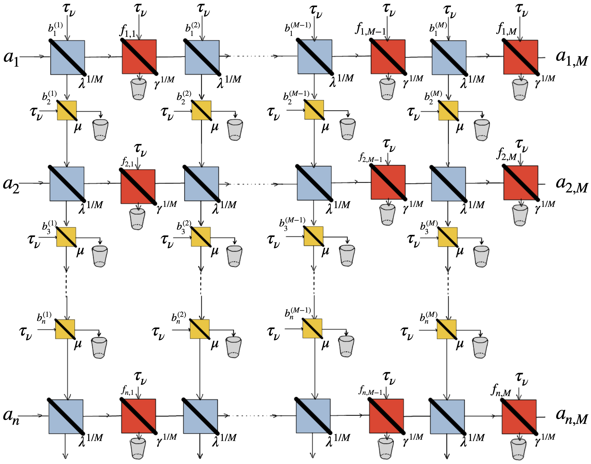
Figure 7: Depiction of the quantum memory channel which models both memory and memoryless noise. In contrast to the model presented in Figure 6, here we have also the red beam splitters of transmissivity $\gamma^{1/M}$ which models the presence of memoryless contribution to the noise. This addition, while it does not substantially affect the mathematical structure of the model, captures the possibility of having different kinds of noise effects on the fibre at the same time, such as scattering, which could enable memory effects, and absorption, which may be memoryless.

This simple model captures the possibility of having the communication line interacting with a multi-mode system, where effectively there are two independent noise effects acting on different timescales. For example, one may think of the memory effects to be due to scattering and the memoryless noise to be due to absorption. Since at the end we will see that the memory channel can be written as a tensor product of attenuators, by the composition rules for attenuators, the capacities of this enhanced model are also completely computable. In particular, it follows that the advantage on the quantum capacity might remain, if $\gamma$ is sufficiently large. If $\nu=0$, the advantage due to memory effects on one-way qubit transmission remains if and only if $\gamma>\frac{1}{2}$, while the two-way quantum capacity can be non-zero as soon as $\gamma\geq\frac{\nu}{\nu+1}$.

In concrete, we modify the model by introducing new modes $\mathbf{f}$ as depicted in Fig. 7, i.e.

$$\mathbf{a} \coloneqq(a_{1},\,a_{2},\ldots,\,a_{n})^{T}\,,$$ (S151)

$$\mathbf{a_{M}} \coloneqq(a_{1,M},\,a_{2,M},\ldots,\,a_{n,M})^{T}\,,$$

$$\mathbf{b} \coloneqq(b_{1}^{(1)},\,b_{1}^{(2)},\ldots,\,b_{1}^{(M)},\,b_{2}^{(1)},\,b_{2}^{(2)},\ldots,\,b_{2}^{(M)},\ldots,\,b_{n}^{(1)},\,b_{n}^{(2)},\ldots,\,b_{n}^{(M)})^{T}\,,$$

$$\mathbf{f} \coloneqq(f_{1,1},f_{1,2},\ldots,\,f_{1,M-1},f_{1,M},\ldots,\,f_{n-1,1},\,f_{n,2},\ldots,\,f_{n,M-1},f_{n,M})^{T}\,,$$

one can modify (S39) as

$$\mathbf{a_{M}}=A^{(M,n,\lambda,\mu,\gamma)}\mathbf{a}+E^{(M,n,\lambda,\mu,\gamma)}\mathbf{b}+F^{(M,n,\lambda,\mu,\gamma)}\mathbf{f}\,,$$ (S152)

where $A^{(M,n,\lambda,\mu,\gamma)}$ is an $n\times n$ real matrix, $E^{(M,n,\lambda,\mu,\gamma)}$ is an $n\times nM$ real matrix, and $F^{(M,n,\lambda,\mu,\gamma)}$ is an $n\times nM$ real matrix which satisfy

$$A^{(M,n,\lambda,\mu,\gamma)}{A^{(M,n,\lambda,\mu,\gamma)}}^{T}+E^{(M,n,\lambda,\mu,\gamma)}{E^{(M,n,\lambda,\mu,\gamma)}}^{T}+F^{(M,n,\lambda,\mu,\gamma)}{F^{(M,n,\lambda,\mu,\gamma)}}^{T}=\mathbb{1}_{n\times n}\,,$$ (S153)

thanks to (S37). By following the same steps of the proof of Theorem S8, we get again

$$\chi_{\Phi_{\lambda,\mu,\nu,\gamma}^{(M,n)}(\rho^{(n)})}(\mathbf{z}) \coloneqq\operatorname{Tr}\left[\Phi_{\lambda,\mu,\nu,\gamma}^{(M,n)}(\rho^{(n)})\,e^{\mathbf{a}^{\dagger}\mathbf{z}-\mathbf{z}^{\dagger}\mathbf{a}}\right]$$ (S154)

$$=\chi_{\rho^{(n)}}\left({A^{(M,n,\lambda,\mu,\gamma)}}^{T}\mathbf{z}\right)\chi_{\tau_{\nu}^{\otimes nM}}\left({E^{(M,n,\lambda,\mu,\gamma)}}^{T}\mathbf{z}\right)\chi_{\tau_{\nu}^{\otimes nM}}\left({F^{(M,n,\lambda,\mu,\gamma)}}^{T}\mathbf{z}\right)$$

$$=\chi_{\rho^{(n)}}\left({A^{(M,n,\lambda,\mu,\gamma)}}^{T}\mathbf{z}\right)e^{-(\nu+\frac{1}{2})\mathbf{z}^{\dagger}(\mathbb{1}_{n\times n}-A^{(M,n,\lambda,\mu,\gamma)}{A^{(M,n,\lambda,\mu,\gamma)}}^{T})\mathbf{z}}\qquad\forall\,\mathbf{z}\in\mathbb{C}^{n}\,,$$

And the analysis continues as in the proof of Theorem S8. We are left to specify $A^{(M,n,\lambda,\mu,\gamma)}$ in the modified model. By exploiting (S11) and the notation in Fig. 7, we derive the following passive transformation:

$$a_{i,j} =\sqrt{\gamma^{1/M}}\sqrt{\lambda^{1/M}}\,a_{i,j-1}+\sqrt{\gamma^{1/M}}\sqrt{1-\lambda^{1/M}}\,m_{i-1,j}+\sqrt{1-\gamma^{1/M}}\,f_{i,j-1}\,,$$ (S155)

$$m_{i,j} =-\sqrt{1-\mu}\,b_{i+1}^{(j)}+\sqrt{\mu\lambda^{1/M}}\,m_{i-1,j}-\sqrt{\mu(1-\lambda^{1/M})}\,a_{i,j-1}\,,$$

where the transmissivity $\gamma$ is associated to memoryless noise. By defining $\tilde{a}_{i,j}\coloneqq\gamma^{-j/M}a_{i,j}$, and $\tilde{m}_{i,j}\coloneqq\gamma^{-(j-1)/M}m_{i,j}$ we obtain

$$\tilde{a}_{i,j} \simeq\sqrt{\lambda^{1/M}}\,\tilde{a}_{i,j-1}+\sqrt{1-\lambda^{1/M}}\,\tilde{m}_{i-1,j}\,,$$ (S156)

$$\tilde{m}_{i,j} \simeq\sqrt{\mu\lambda^{1/M}}\,\tilde{m}_{i-1,j}-\sqrt{\mu(1-\lambda^{1/M})}\,\tilde{a}_{i,j-1}\,,$$

which are the recurrence relations for the model at $\gamma=1$. We immediately get

$$A^{(M,n,\lambda,\mu,\gamma)}=\sqrt{\gamma}A^{(M,n,\lambda,\mu,1)}=\sqrt{\gamma}A^{(M,n,\lambda,\mu)}$$ (S157)

and therefore

$$\bar{A}_{i,h}^{(n,\lambda,\mu,\gamma)}\coloneqq\lim\limits_{M\rightarrow\infty}A_{i,h}^{(M,n,\lambda,\mu,\gamma)}=\sqrt{\gamma}\bar{A}_{i,h}^{(n,\lambda,\mu)}\,.$$ (S158)

This means that this modification of the model is equivalent to placing a thermal attenuator with transmissivity $\gamma$ before or after the memory channel. Mathematically, the square of the absolute values of the singular values of $\bar{A}_{i,h}^{(n,\lambda,\mu,\gamma)}$ are obtained by rescaling those of $\bar{A}_{i,h}^{(n,\lambda,\mu)}$ by $\gamma$. It follows that as long as $\gamma>1/2$ and for $\nu=0$, there are values of $\mu$ and $\lambda$ such that the quantum capacity is still non-zero. In particular $\gamma\lambda$, which can be thought as the effective attenuation on the fibre, could be less than $1/2$ while the quantum capacities are still non zero. A similar observation holds for the two-way capacities. If there were no memory effects, the two-way quantum capacity would be zero if and only if $\gamma\lambda\leq\frac{\nu}{\nu+1}$, while in our model it can be still non-zero even if the inequality is satisfied.

References

• [1] M. A. Nielsen and I. L. Chuang. Quantum Computation and Quantum Information: 10th Anniversary Edition. Cambridge University Press, Cambridge, 2010.
• [2] S. Wehner, D. Elkouss, and R. Hanson. Quantum internet: A vision for the road ahead. Science, 362:eaam9288, 10 2018.
• [3] S. Pirandola et al. Advances in quantum cryptography. Advances in Optics and Photonics, 12(4):1012–1236, 2020.
• [4] C. H. Bennett. Quantum cryptography: public key distribution and coin tossing. In Proc. IEEE International Conference on Computers, Systems and Signal Processing, Bangalore, India, pages 175–179, 1984.
• [5] J. S. Sidhu et al. Advances in space quantum communications. IET Quantum Communication, 2(4):182–217, 2021.
• [6] J. I. Cirac, A. K. Ekert, S. F. Huelga, and C. Macchiavello. Distributed quantum computation over noisy channels. Physical Review A, 59:4249–4254, 1999.
• [7] A. Broadbent, J. Fitzsimons, and E. Kashefi. Universal blind quantum computation. 2009 50th Annual IEEE Symposium on Foundations of Computer Science, 2009.
• [8] H.-J. Briegel, W. Dür, J. I. Cirac, and P. Zoller. Quantum repeaters: The role of imperfect local operations in quantum communication. Physical Review Letters, 81:5932–5935, 1998.
• [9] W. J. Munro, K. Azuma, K. Tamaki, and K. Nemoto. Inside quantum repeaters. IEEE Journal of Selected Topics in Quantum Electronics, 21(3):78–90, 2015.
• [10] F. A. Mele, L. Lami, and V. Giovannetti. Restoring quantum communication efficiency over high loss optical fibers. Physical Review Letters, 129:180501, 2022.
• [11] F. A. Mele, L. Lami, and V. Giovannetti. Quantum optical communication in the presence of strong attenuation noise. Physical Review A, 106:042437, 2022.
• [12] F. Caruso, V. Giovannetti, C. Lupo, and S. Mancini. Quantum channels and memory effects. Reviews of Modern Physics, 86:1203–1259, 2014.
• [13] V. Giovannetti. A dynamical model for quantum memory channels. J. Phys. A: Math. Gen., 38(50):10989–11005, 2005.
• [14] K. Banaszek, A. Dragan, W. Wasilewski, and C. Radzewicz. Experimental demonstration of entanglement-enhanced classical communication over a quantum channel with correlated noise. Physical Review Letters, 92:257901, 2004.
• [15] J. Ball, A. Dragan, and K. Banaszek. Exploiting entanglement in communication channels with correlated noise. Physical Review A, 69:042324, 2004.
• [16] C. Lupo, V. Giovannetti, and S. Mancini. Capacities of lossy bosonic memory channels. Phys. Rev. Lett., 104:030501, Jan 2010.
• [17] C. Lupo, V. Giovannetti, and S. Mancini. Memory effects in attenuation and amplification quantum processes. Phys. Rev. A, 82:032312, Sep 2010.
• [18] G. De Palma, A. Mari, and V. Giovannetti. Classical capacity of gaussian thermal memory channels. Phys. Rev. A, 90:042312, Oct 2014.
• [19] M. M. Wilde. Quantum Information Theory. Cambridge University Press, 2nd edition, 2017.
• [20] S. Khatri and M. M. Wilde. Principles of quantum communication theory: A modern approach, 2020.
• [21] L. Lami, M. B. Plenio, V. Giovannetti, and A. S. Holevo. Bosonic quantum communication across arbitrarily high loss channels. Physical Review Letters, 125:110504, 2020.
• [22] F. A. Mele, L. Lami, and V. Giovannetti. Maximum tolerable excess noise in CV-QKD and improved lower bound on two-way capacities. Preprint arXiv:2303.12867, 2023.
• [23] C. M. Caves and P. D. Drummond. Quantum limits on bosonic communication rates. Reviews of Modern Physics, 66:481–537, 1994.
• [24] A. Serafini. Quantum Continuous Variables: A Primer of Theoretical Methods. CRC Press, Taylor & Francis Group, Boca Raton, USA, 2017.
• [25] A. S. Holevo and R. F. Werner. Evaluating capacities of bosonic Gaussian channels. Physical Review A, 63:032312, 2001.
• [26] V. Giovannetti, S. Lloyd, L. Maccone, and P. W. Shor. Entanglement assisted capacity of the broadband lossy channel. Physical Review Letters, 91:047901, 2003.
• [27] V. Giovannetti, S. Lloyd, L. Maccone, and P. W. Shor. Broadband channel capacities. Physical Review A, 68:062323, 2003.
• [28] S. Pirandola, R. Laurenza, C. Ottaviani, and L. Banchi. Fundamental limits of repeaterless quantum communications. Nature Communications, 8(1):15043, 2017.
• [29] M. Rosati, A. Mari, and V. Giovannetti. Narrow bounds for the quantum capacity of thermal attenuators. Nature Communications, 9(1):4339, 2018.
• [30] K. Sharma, M. M. Wilde, S. Adhikari, and M. Takeoka. Bounding the energy-constrained quantum and private capacities of phase-insensitive bosonic Gaussian channels. New Journal of Physics, 20(6):063025, 2018.
• [31] K. Noh, V. V. Albert, and L. Jiang. Quantum capacity bounds of Gaussian thermal loss channels and achievable rates with Gottesman-Kitaev-Preskill codes. IEEE Transactions on Information Theory, 65(4):2563–2582, 2019.
• [32] K. Noh, S. Pirandola, and L. Jiang. Enhanced energy-constrained quantum communication over bosonic Gaussian channels. Nature Communications, 11(1):457, 2020.
• [33] M. Fanizza, F. Kianvash, and V. Giovannetti. Estimating quantum and private capacities of gaussian channels via degradable extensions. Physical Review Letters, 127:210501, 2021.
• [34] S. Pirandola, R. García-Patrón, S. L. Braunstein, and S. Lloyd. Direct and reverse secret-key capacities of a quantum channel. Physical Review Letters, 102:050503, 2009.
• [35] C. Ottaviani et al. Secret key capacity of the thermal-loss channel: improving the lower bound. In Mark T. Gruneisen, Miloslav Dusek, and John G. Rarity, editors, Quantum Information Science and Technology II, volume 9996, page 999609. International Society for Optics and Photonics, SPIE, 2016.
• [36] Y. Tamura, H. Sakuma, K. Morita, M. Suzuki, Y. Yamamoto, K. Shimada, Y. Honma, K. Sohma, T. Fujii, and T. Hasegawa. The first 0.14-db/km loss optical fiber and its impact on submarine transmission. J. Lightwave Technol., 36(1):44–49, 2018.
• [37] M.-J. Li and T. Hayashi. Chapter 1 - advances in low-loss, large-area, and multicore fibers. In A. E. Willner, editor, Optical Fiber Telecommunications VII, pages 3–50. Academic Press, 2020.
• [38] V. Giovannetti and G. M. Palma. Master equations for correlated quantum channels. Phys. Rev. Lett., 108:040401, Jan 2012.
• [39] F. Avram. On bilinear forms in Gaussian random variables and Toeplitz matrices. Probab. Theory Related Fields, 79(1):37–45, 1988.
• [40] S. V. Parter. On the distribution of the singular values of Toeplitz matrices. Linear Algebra Appl., 80:115–130, 1986.
• [41] M. M. Wolf, D. Pérez-García, and G. Giedke. Quantum capacities of bosonic channels. Physical Review Letters, 98:130501, 2007.
• [42] L. Lami, K. K. Sabapathy, and A. Winter. All phase-space linear bosonic channels are approximately Gaussian dilatable. New Journal of Physics, 20(11):113012, 2018.
• [43] C. D. Cushen and R. L. Hudson. A quantum-mechanical central limit theorem. Journal of Applied Probability, 8(3):454–469, 1971.
• [44] C. H. Bennett, G. Brassard, C. Crépeau, R. Jozsa, A. Peres, and W. K. Wootters. Teleporting an unknown quantum state via dual classical and Einstein-Podolsky-Rosen channels. Physical Review Letters, 70:1895–1899, 1993.
• [45] N. Davis, M. E. Shirokov, and M. M. Wilde. Energy-constrained two-way assisted private and quantum capacities of quantum channels. Physical Review A, 97:062310, 2018.
• [46] K. Goodenough, D. Elkouss, and S. Wehner. Assessing the performance of quantum repeaters for all phase-insensitive Gaussian bosonic channels. New Journal of Physics, 18(6):063005, 2016.
• [47] M. Takeoka, S. Guha, and M. M. Wilde. Fundamental rate-loss tradeoff for optical quantum key distribution. Nature Communications, 5(1):5235, 2014.
• [48] M. M. Wilde, M. Tomamichel, and M. Berta. Converse bounds for private communication over quantum channels. IEEE Transactions on Information Theory, 63(3):1792–1817, 2017.
• [49] M. Takeoka, S. Guha, and M. M. Wilde. The squashed entanglement of a quantum channel. IEEE Transactions on Information Theory, 60(8):4987–4998, 2014.
• [50] S. Pirandola, S. L. Braunstein, R. Laurenza, C. Ottaviani, T. P. W. Cope, G. Spedalieri, and L. Banchi. Theory of channel simulation and bounds for private communication. Quantum Science and Technology, 3(3):035009, 2018.
• [51] G. Wang, C. Ottaviani, H. Guo, and S. Pirandola. Improving the lower bound to the secret-key capacity of the thermal amplifier channel. The European Physical Journal D, 73(1):17, 2019.
• [52] L. Lami, S. Khatri, G. Adesso, and M. M. Wilde. Extendibility of bosonic Gaussian states. Physical Review Letters, 123:050501, 2019.
• [53] F. Caruso, V. Giovannetti, and A. S. Holevo. One-mode bosonic Gaussian channels: a full weak-degradability classification. New Journal of Physics, 8(12):310–310, 2006.
• [54] A. S. Holevo. Probabilistic and Statistical Aspects of Quantum Theory. Publications of the Scuola Normale Superiore. Scuola Normale Superiore, Pisa, Italy, 2011.
• [55] G. Szegő. Beiträge zur Theorie der Toeplitzschen Formen. Math. Z., 6(3):167–202, 1920.
• [56] U. Grenander and G. Szegő. Toeplitz forms and their applications. Chelsea Publishing Co., New York, second edition, 1984.
• [57] Robert M. Gray. Toeplitz and circulant matrices: A review. Foundations and Trends® in Communications and Information Theory, 2(3):155–239, 2006.
• [58] A. Böttcher and S. M. Grudsky. Toeplitz matrices, asymptotic linear algebra, and functional analysis. Birkhäuser Verlag, Basel, 2000.
• [59] A. Böttcher and S. M. Grudsky. Spectral properties of banded Toeplitz matrices. Society for Industrial and Applied Mathematics (SIAM), Philadelphia, PA, 2005.
• [60] C. Garoni and S. Serra-Capizzano. Generalized locally Toeplitz sequences: theory and applications. Vol. I. Springer, Cham, 2018.
• [61] S. M. Grudsky. Eigenvalues of larger Toeplitz matrices: the asymptotic approach. Lecture notes, 2010.
• [62] Ludovico Lami and Mark M. Wilde. Exact solution for the quantum and private capacities of bosonic dephasing channels. Nature Photonics, 17:525–530, June 2023.
• [63] Y.S. Chow and H. Teicher. Probability theory: Independence interchangeability martingales. 2012.