On Continuity of Robust and Accurate Classifiers

Abstract

The reliability of a learning model is key to the successful deployment of machine learning in various applications. Creating a robust model, particularly one unaffected by adversarial attacks, requires a comprehensive understanding of the adversarial examples phenomenon. However, it is difficult to describe the phenomenon due to the complicated nature of the problems in machine learning. It has been shown that adversarial training can improve the robustness of the hypothesis. However, this improvement comes at the cost of decreased performance on natural samples. Hence, it has been suggested that robustness and accuracy of a hypothesis are at odds with each other. In this paper, we put forth the alternative proposal that it is the continuity of a hypothesis that is incompatible with its robustness and accuracy. In other words, a continuous function cannot effectively learn the optimal robust hypothesis. To this end, we will introduce a framework for a rigorous study of harmonic and holomorphic hypothesis in learning theory terms and provide empirical evidence that continuous hypotheses does not perform as well as discontinuous hypotheses in some common machine learning tasks. From a practical point of view, our results suggests that a robust and accurate learning rule would train different continuous hypotheses for different regions of the domain. From a theoretical perspective, our analysis explains the adversarial examples phenomenon as a conflict between the continuity of a sequence of functions and its uniform convergence to a discontinuous function.

I Introduction

Adversarial examples are amongst the most discussed malicious phenomenon in training robust machine learning models. The phenomenon refers to a situation where a trained model is fooled to return an undesirable output on particular inputs that an adversary carefully crafts. The ease of generating these examples and its abundance in most applications of supervised machine learning have posed serious challenges in adoption of machine learning in a safe and secure manner. For example, the phenomenon would allow a malicious actor to alter the predictions of a cloud-based machine learning model[1], or bypass a face-detection model through makeup[2]. Thus, many studies on the possible causes and effects of this phenomenon have been conducted.

While there is no consensus on the reasons behind the emergence of these examples, many facets of the phenomenon have been revealed. For example, Szegedy et al. show that adversarial perturbations are not random and they generalize to other models[3], or Goodfellow et al. indicate that linear approximations of the model around a test sample is an effective surrogate for the model in the generation of adversarial examples[4]. A known aspect of adversarial examples is that a hypothesis can be trained on its own adversarial examples and improve in robustness. The efficient implementation of an adversarial attack by Goodfellow et al. was the first method that made adversarial training feasible[4]. Many related proposals and improvements have been proposed since, and adversarial training is regarded as the most effective defence method in the community[5].

However, it has been shown that adversarial training suffers from a few shortcomings. As an example, it has been observed that adversarial training has a negative effect on the standard performance of the model[6]. There are conflicting views regarding this observation. A popular explanation is that robustness and accuracy are in opposition, and binary classification problems have been synthesized in which standard accuracy and robustness are at odds with each other[7]. There is a study that finds negative correlation between the robustness and standard accuracy of adversarially trained models[8]. In contrast, there are others that challenge this idea. For example, there is evidence that some of the standard training sets are separable[9], and that robust linear classifiers appear to be possible[10]. Moreover, adversarially trained hypotheses do not generalize to unseen attacks[11]. This issue has severely hindered the effectiveness of adversarial training[5]. As a result, studies have been conducted on mixing different adversarial attacks in hope of training a more robust hypothesis[12].

Many ideas in the related literature are implicitly or explicitly based on the assumption that the optimal robust hypothesis, if existing, is bounded and Lipschitz continuous[13, 14, 15]. There is a sentiment that a complete hypothesis space such as artificial neural networks (ANN) should be able to represent the robust hypothesis given enough training samples[4, 16], and others are hopeful that an inept understanding of deep ANNs would bring about a solution for the phenomenon[17]. The assumption of existence of a continuous robust and accurate hypothesis is an idea that conforms to intuition. We believe however that this assumption might not be warranted. We argue that continuity of a robust and accurate classifier is a strong assumption and it is not true in common applications. In this paper, we are aiming to describe a framework for the study of the discontinuities of a robust and accurate hypothesis. Learning rules that regularize the norm of the gradient of the hypothesis play an important role in our framework. A part of the framework is concerned with detecting adversarial examples of a classifier.

Regularization of the norm of the gradient of the hypothesis is a technique that have been shown to be effective in training robust hypothesis[18, 19, 20]. The idea is mostly based on the fact that if we approximate a hypothesis around a test sample by a linear function, that linear function should be as constant as possible. In [21] for example, Jacobian norm has been used to improve the robustness of the linear approximation. An empirical study showed that regularized artificial neural networks exhibit robustness to transferred adversarial examples and that human volunteers find the misclassifications more interpretable[22]. The concentration of the distribution of the the gradient of the loss function has been found to be related to the robustness of stochastic neural networks[23]. Gradient regularization has been used to decrease the effect of transferability of adversarial examples between models[24].

There are also approaches that try to detect adversarial examples, a task that proved to be harder than it seemed at first[25]. An empirical study of different methods of detection can be found in [26]. It was shown in [27] that the distribution of adversarial examples differs substantially from the distribution of natural training samples. This difference was shown by performing statistical testing and reinforced by the observation that a classifier can be trained to detect the adversarial examples produced by an attack. The activation of convolutional layers has been used to detect the adversarial examples [28]. Similarly, in [29] the histogram created from the activations of the hidden layer of an artificial neural network is used to train a classifier for detecting adversarial examples. It was shown by [30] that correctly classified examples tend to have greater maximum softmax probabilities compared to erroneously classified and out-of-distribution examples.

A summary of our contributions are:

• We introduce weakly-harmonic learning rules that use the Dirichlet energy of the hypothesis as a reguralizer. By doing so, we are able to apply the methods of variational calculus and turn the learning problem into a partial differential equation. We will use this construct as a model to study the effects of regularization of the norm of the gradient of the hypothesis.

• We further introduce the space of weakly-harmonic hypotheses as an abstraction for a solution to a weakly-harmonic learning problem, and provide a convenient representation for these hypotheses.

• By extending the domain of weakly-harmonic hypotheses into the complex space, we present discontinuities in the optimal hypothesis as an explanation for the existence of adversarial regions in the domain of analytic hypothesis. We introduce the space of holomorphic hypotheses and propose a systematic approach for determining the discontinuity of an optimal classifier.

• We propose a convolutional architecture for constructing weakly-harmonic and holomorphic classifiers and empirically show that there is a fundamental limit on the performance of continuous hypotheses in common image classification tasks.

We can summarize the significance of our contributions in two parts. First, our results suggests that a robust and accurate hypothesis is a collection of hypotheses that are specialized for different regions of the domain. We further lay a theoretical basis for constructing such hypotheses. Second, by relating the adversarial regions to established concepts in analysis of holomorphic functions, we open a path to a rigorous analysis of the adversarial examples phenomenon that can freely move between the study of the geometrical and the algebraic properties of the hypothesis.

II Preliminaries

II-A Dirichlet Hypothesis Spaces

Analyses in machine learning are done under some framework of learning. We will conduct our analysis under the framework of probably approximately correct (PAC) learning[31, chapter 3]. The aim of PAC learnability is to bound the true generalization error of the trained hypothesis given the observed generalization error on test samples.

Definition II.1 (PAC hypothesis).

Suppose that $\mathcal{X}\subseteq\mathbb{R}^{n}$ is a domain, $\mathcal{F}(\mathcal{X})$ is a set of functions defined on $\mathcal{X}$ and $t:\mathcal{X}\to\mathbb{R}^{m}$ is some function. Consider a function $\mathrm{loss}:\mathcal{X}\times\mathcal{F}(\mathcal{X})\to\mathbb{R}$ that measures how bad of a fit some hypothesis $h\in\mathcal{F}(\mathcal{X})$ is with respect to $t$ for some $x\in\mathcal{X}$, and a random variable $X$ supported on $\mathcal{X}$. Then $h$ is PAC for $X$ if some $\epsilon,\delta\in(0,1)$ exists for which

$$\mathbb{P}_{X}\big{[}\mathrm{loss}(x,h)\leq\epsilon\big{]}\geq 1-\delta.$$ (1)

If $h$ is furthermore PAC for all random variables $X$, then $h$ is PAC on $\mathcal{X}$.

A learning rule for $\mathcal{F}(\mathcal{X})$ is a search algorithm for finding hypotheses in $\mathcal{F}(\mathcal{X})$. We will refer to a set of functions $\mathcal{F}(\mathcal{X})$ as a PAC learnable hypothesis space when a learning rule exists that given a large enough training set $S\subset\mathcal{X}$ is guaranteed to find a hypothesis $h\in\mathcal{F}(\mathcal{X})$ that is PAC on $\mathcal{X}$. PAC learnability implies that an integer-valued function exists that specifies the size of the training set for any $\epsilon,\delta$ which is called the sample complexity of $\mathcal{F}$. Naturally, as we demand smaller values for $\epsilon$ and $\delta$, we require larger training sets. From here onward, we will use $\mathrm{loss}(x,h;t)$ to indicate that the target of the loss function is $t$.

However, PAC learnable hypothesis spaces are too restrictive in terms of representation power. As a consequence, relaxations of PAC learnability are introduced. One such relaxation is nonuniform learnability[31, definition 7.1]. Nonuniform learnability allows for sample complexities that further are dependent on the target $t$. Many useful hypothesis spaces, such as polynomials, are nonuniform learnable[31, example 7.1].

Definition II.2 (modes of convergence).

Consider a sequence of functions $\{h_{k}:\mathcal{X}\to\mathbb{R}^{n}\}_{1}^{\infty}$ and a function $h:\mathcal{X}\to\mathbb{R}^{n}$.

1. $\{h_{k}\}_{1}^{\infty}$ is converging pointwise to $h$ if for every $\epsilon>0$, a natural number $K(x)$ exists for which

   $$|h(x)-h_{k}(x)|<\epsilon,\quad k>K(x).$$ (2)

2. $\{h_{k}\}_{1}^{\infty}$ is uniformly converging to $h$ if for every $\epsilon>0$ some $K\in\mathbb{N}$ exists for which

   $$\sup_{x\in\mathcal{X}}|h(x)-h_{k}(x)|<\epsilon,\quad k>K.$$ (3)

$h$ is called the pointwise limit of $\{h_{k}:\mathcal{X}\to\mathbb{R}^{n}\}_{1}^{\infty}$ in both cases.

The reason that we are interested in the modes of convergence of $\{h_{k}\}_{1}^{\infty}$ is that certain properties of hypotheses in the sequence may or may not get passed to its pointwise limit $h$, depending on its mode of convergence[32, chapter 11]. Specifically, if every $h_{k}$ is continuous, then $h$ is continuous when the convergence is uniform, but not when it is pointwise. On the other hand, there is no reason to believe that the differentiability of $h_{k}$ would pass to $h$, even when the convergence is uniform.

The learning rules that we will study here fall under the paradigm of structural risk minimization[31, chapter 7.2]. In structural risk minimization, other than minimizing the risk (loss) of the hypothesis, we will assign a weight to every $\mathcal{F}_{k}$ depending on the complexity of $\mathcal{F}_{k}$ and penalize the hypothesis based on this weight function. The paradigm is very similar to regularized risk minimization[31, chapter 13], but structural risk minimization would better describe the learning rules that we are interested in.

We can decompose the loss of $h$ into the estimation error $\epsilon_{\mathrm{est}}$ and the approximation error $\epsilon_{\mathrm{app}}$[31, section 5.2]. The approximation error is the part of the loss that is caused by limitations of $\mathcal{F}$. For example, there is a limit on how good a linear function can fit to a sinusoidal function no matter the size of $S$. The estimation error is the other part of the loss that is caused by insufficient training samples in $S$. Formally,

$$\mathrm{loss}(x,h;t)=\epsilon_{\mathrm{est}}+\epsilon_{\mathrm{app}}.$$ (4)

In our discussion, we will separate a representation of a hypothesis $h$ from the hypothesis itself. In other words, it is possible for a hypothesis to have multiple equal representations. These representations can come in many forms, they could be a summation of bases, a stochastic process, or a deep neural network. Here, we are concerned with the series representations of $h$.

Definition II.3 (series representation).

A hypothesis $h:\mathcal{X}\subseteq\mathbb{C}^{n}\to\mathbb{C}$ has a series representation if and only if a set of non-constant continuous features $\{\varphi_{k}:\mathcal{X}\to\mathbb{C}\}_{1}^{K}$ exists for which:

$$h(x)=b+\sum_{k=1}^{K}w_{k}\varphi_{k}(x),$$ (5)

for some set of coefficients $\{w_{k}\}_{1}^{K}\subset\mathbb{C}$ and some bias term $b\in\mathbb{C}$.

The use of $\mathbb{C}$ in the definition is to keep consistency between the sections of the paper. In this section we would not discuss any complex-valued hypothesis and it is safe to substitute $\mathbb{C}$ with $\mathbb{R}$. We have deliberately separated $b$ and $w$ because $b$ does not affect the derivatives of $h$. An example of a series representation is a power series representation, e.g. the Taylor expansion of $h$ around some point. There is a set of short-hand notations called multi-index[33, page 3] notation that will be very handy in dealing with power series in high dimensions.

Definition II.4 (multi-index notation).

Suppose that $\alpha=(\alpha_{1},\cdots,\alpha_{n})\in\mathbb{N}^{n}$ is a sequence of $n$ natural numbers and $x\in\mathbb{R}^{n}$. Then,

$$x^{\alpha} =x_{1}^{\alpha_{1}}x_{2}^{\alpha_{2}}\cdots x_{n}^{\alpha_{n}},$$ (6)

$$\partial x^{\alpha} =\partial x_{1}^{\alpha_{1}}\partial x_{2}^{\alpha_{2}}\cdots\partial x_{n}^{\alpha_{n}},$$ (7)

$$\|\alpha\|_{p} =\big{(}\sum_{j=1}^{n}\alpha_{j}^{p}\big{)}^{\frac{1}{p}},$$ (8)

$$\alpha! =\alpha_{1}!\alpha_{2}!\cdots\alpha_{n}!.$$ (9)

Before we continue with the introduction of the hypothesis space, it is necessary to introduce the Dirichlet energy of a function[34].

Definition II.5 (Dirichlet energy of $h$).

The Dirichlet energy $E[h]$ of a differentiable function $h:\mathcal{X}\rightarrow\mathbb{R}$ is a measure of its variability and is computed as:

$$E[h]=\int_{\mathcal{X}}\|\nabla h(x)\|^{2}\,\mathrm{d}V(x),$$ (10)

in which $\mathrm{d}V(x)$ is the differential element of volume of $\mathcal{X}$.

Definition II.6 (Dirichlet space).

The Dirichlet space $\mathcal{D}(\mathcal{X})$ consists of functions $h:\mathcal{X}\rightarrow\mathbb{R}$ with finite Dirichlet energy:

$$h\in\mathcal{D}(\mathcal{X})\iff E[h]<\infty.$$ (11)

Considering the definition of Dirichlet energy, we can see all methods that regularize the norm of the gradient are in fact minimizing a weighted generalization of the Dirichlet energy. So it is convenient for us to be able to compute the weighted Dirichlet energy of the series representation of $h$.

Definition II.7 (tuning matrix).

Suppose that $\{\varphi_{k}\}_{1}^{K}\subset\mathcal{D}(\mathcal{X})$ is a set of features and that $q:\mathcal{X}\to\mathbb{R}_{+}$ is some weight function. The tuning matrix $\Sigma$ of $\{\varphi_{k}\}_{1}^{K}$ is a $K\times K$ Hermitian matrix computed as:

$$\Sigma_{ij}=\int_{\mathcal{X}}\nabla\varphi_{i}(x)\cdot\nabla\varphi_{j}(x)\,q(x)\,\mathrm{d}V(x).$$ (12)

Having computed the tuning matrix of $\{\varphi_{k}\}_{1}^{K}$, it would be easy to compute the weighted Dirichlet energy of $h$. The calculations would be more efficient if $\Sigma$ illustrates some structure.

Definition II.8 (weakly-harmonic features).

A set of features $\{\varphi_{k}\}_{1}^{K}\subset\mathcal{D}(\mathcal{X})$ is weakly-harmonic if its tuning matrix $\Sigma$ is the identity matrix $I$.

Theorem II.1.

Suppose that $\{\varphi_{k}\}_{1}^{K}$ is weakly-harmonic with $q(x)=1$ and $h\in\mathcal{D}(\mathcal{X})$ has a series representation in $\{\varphi_{k}\}_{1}^{K}$. Then,

$$E[h]=\sum_{k=1}^{K}|w_{k}|^{2}.$$ (13)

Theorem II.1 can be generalized to arbitrary $q(x)$ and weighted Dirichlet energy with little to no effort. The case of $q(x)=1$ is special because according to the Dirichlet principle[34], any function $h\in\mathcal{D}(\mathcal{X})$ that is only constrained on the boundary $\partial\mathcal{X}$ of $\mathcal{X}$ and has minimal Dirichlet energy is harmonic, i.e., $\Delta h(x)=0$. Theorem II.1 is where the line between structural and regularized risk minimization gets blurry in the learning rules that we are considering.

Theorem II.2.

Suppose that $\{\varphi_{k}\}_{1}^{K}\subset\mathcal{D}(\mathcal{X})$ is not weakly-harmonic. Then $\{\varphi_{k}\}_{1}^{K}$ can be transformed into a set of weakly-harmonic features $\{\varphi^{*}_{k}\}_{1}^{K}$ by:

$$\varphi^{*}(x)=\Sigma^{-\frac{1}{2}}\varphi(x).$$ (14)

According to Theorem II.2, any finite sequence of features with finite Dirichlet energy can be transformed to a set of weakly-harmonic features. However, the hypothesis spaces that can only accommodate a finite number of features are not very interesting from the perspective of learning. In the case of an infinite tuning matrix, it would be necessary for $\Sigma$ to be diagonalizable in order to compute $\Sigma^{-\frac{1}{2}}$.

Given that we want to study the effects of regularization of the norm of the gradient during training, we have to limit the hypothesis spaces that we consider to spaces that are suitably integrable in both value and derivatives[35, chapter 7].

Definition II.9 (Sobolev spaces).

The Sobolev space $H^{d}(\mathcal{X})$ is the space of functions $h:\mathcal{X}\to\mathbb{R}$ such that for any multi-index $\alpha$ for which $\|\alpha\|_{1}\leq d$, the partial derivative

$$h^{(\alpha)}(x)=\frac{\partial^{\|\alpha\|_{1}}h}{\partial x^{\alpha}}(x)$$ (15)

exists in the weak sense and is in $L^{2}(\mathcal{X})$.

$L^{2}(\mathcal{X})$ is a Hilbert space of functions with the inner product,

$$f\cdot g=\int_{\mathcal{X}}f(x)\overline{g(x)}\,\mathrm{d}V(x),$$ (16)

in which $\overline{g(x)}$ is the complex-conjugate of $g(x)$[36, section 4.1], and consists of square-integrable functions,

$$h\in L^{2}(\mathcal{X})\iff\|h\|_{L^{2}}=(h\cdot h)^{\frac{1}{2}}<\infty.$$ (17)

The difference between a Hilbert space and an inner product space is that a Hilbert space is complete. In other words, the pointwise limit of any uniformly converging sequence of functions $\{h_{k}\in L^{2}(\mathcal{X})\}_{1}^{\infty}$ is a function inside $L^{2}(\mathcal{X})$[36, theorem 4.1.2]. It would be more appropriate to think of $L^{2}(\mathcal{X})$ as the set of equivalence classes of functions that only differ on a non-measurable subset of $\mathcal{X}$. The weak derivative is a relaxation of the concept of derivative of a function through integration by parts[35, section 7.3]. For example, the Dirac delta is the weak derivative of the Heaviside sign function. The weak derivative would equal the (strong) derivative when $h$ is differentiable.

Definition II.10 (weakly-harmonic problem).

A weakly-harmonic problem is the problem of finding a hypothesis $h\in H^{1}(\mathcal{X})$ that minimizes the Lagrangian $\mathcal{L}$:

$$\mathcal{L}=\frac{1}{2}E[h]+\mathbb{E}_{S}[\mathrm{loss}(x,h;t)],$$ (18)

in which $S$ is some random variable supported on $\mathcal{X}$.

The weakly-harmonic learning problem is the abstraction that we choose to model the learning rules that regularize the norm of the gradient. A more realistic model would replace the Dirichlet energy in the definition with the weighted Dirichlet energy of $h$. However, doing so would introduce complications in the analysis that are out of the scope of this paper.

The form of the optimization problem in equation 18 allows for the use of methods of variational calculus[35, section 11.5]. As a result, we can solve for $h$ without having to first assume a representation for $h$.

Theorem II.3.

Suppose that $h\in H^{2}(\mathcal{X})$ is a solution to a weakly-harmonic learning problem. Then $h$ is a weak solution the following partial differential equation (PDE):

$$\Delta h(x)=s(x)\mathrm{loss}_{h}(x;h,t),$$ (19)

in which $\mathrm{loss}_{h}$ is the variational derivative of $\mathrm{loss}$ with respect to $h$, $s(x)$ is the probability distribution of $S$ and $\Delta$ is the Laplacian operator.

The weak solution is a generalization that makes use of the concept of a weak derivative. The PDE of equation 19 might not have a unique solution when $\mathrm{loss}$ is not convex. Moreover, we only have access to an empirical distribution for $S$. Nevertheless, we propose that the effect of the right hand side of equation 19 can be replaced by some unknown function independent of $h$. Informally, we can see that $\Delta h(x)=0$ when either $s(x)$ or $\mathrm{loss}_{h}(x;h,t)$ vanish. Thus, the optimal solution would be a harmonic function when possible. Otherwise, the optimal solution would not be harmonic and the effects on the optimal solution could be interpreted as some forcing on some harmonic function.

Definition II.11 (weakly-harmonic hypothesis space).

A weakly-harmonic hypothesis space $\mathcal{H}(\mathcal{X})\subseteq H^{2}(\mathcal{X})$ is the set of hypotheses $h$ that are solutions to the following partial differential equation:

$$\Delta h(x) =f(x),$$ (20)

$$\frac{\partial h}{\partial\hat{n}}(x) =g(x)\quad x\in\partial\mathcal{X},$$ (21)

in which $\frac{\partial h}{\partial\hat{n}}(x)$ is the derivative of $h$ in the direction of the normal $\hat{n}$ to the boundary $\partial\mathcal{X}$ and $f,g\in L^{2}(\mathcal{X})$ are some functions.

Thus, we can divide the learning of the solution to a weakly-harmonic learning problem to two problems; one for $f$ and one for $g$. In other words, if we assume that $u\in H^{2}(\mathcal{X})$ is a strong solution to a weakly-harmonic learning problem, then $u$ has a representation in $\mathcal{H}(\mathcal{X})$ by choosing $f(x)=\Delta u(x)$ and $g(x)=\frac{\partial u}{\partial\hat{n}}(x)$. There are many methods for approximating the solutions to the PDE of a weakly-harmonic hypothesis space. Here, we will be solving the PDEs with the help of the Green function of the Laplacian operator[35, chapter 2.4].

Definition II.12 (eigenvalue problem of $\mathcal{H}$).

Suppose that $\mathcal{H}(\mathcal{X})$ is a weakly-harmonic hypothesis space. Then, its corresponding eigenvalue problem is:

$$\Delta\varphi(x) =-\lambda^{2}\varphi(x),$$ (22)

$$\frac{\partial\varphi}{\partial\hat{n}}(x) =0\quad x\in\partial\mathcal{X}.$$ (23)

Theorem II.4.

Suppose that $\mathcal{H}(\mathcal{X})$ is a weakly-harmonic hypothesis space, $\partial\mathcal{X}$ is $C^{2}$ and that the eigenvalue problem of $\mathcal{H}(\mathcal{X})$ is solvable by separation of variables. Then,

1. $\mathcal{H}(\mathcal{X})$ is nonuniform learnable.

2. every $h\in\mathcal{H}(\mathcal{X})$ has a series representation in $\{\varphi_{k}\}_{1}^{\infty}$ of eigenfunctions of the eigenvalue problem of $\mathcal{H}$.

3. The tuning matrix $\Sigma$ of $\{\varphi_{k}\}_{1}^{\infty}$ is diagonal.

$C^{2}$ is a constraint on the smoothness of $\partial\mathcal{X}$. Informally, if $\partial\mathcal{X}$ is $C^{2}$ then a twice differentiable function $\rho$ exists that is zero for every $x\in\partial\mathcal{X}$ while $\nabla\rho(x)\neq 0$. Theorem II.4 provides us with the minimum requirements needed to make use of $\mathcal{H}(\mathcal{X})$ in expected risk minimization problems. Given a representation and the fact that $\mathcal{H}(\mathcal{X})$ is nonuniform learnable, any expected risk minimization[31, chapter 1] algorithm would suffice to train a hypothesis. Nevertheless, for a concrete hypothesis space, we have to first choose some $\mathcal{X}$. Even though the boundary of $[0,1]^{n}$ is not $C^{2}$, the eigenvalue problem of $\mathcal{H}([0,1]^{n})$ is solvable by separation of variables. The issue of smoothness of the boundary of the hypercube would not pose a problem in practice and we can safely assume that theorem II.4 applies to $\mathcal{H}([0,1]^{n})$.

Theorem II.5.

Consider the domain $\omega=[0,\pi]^{n}$. The solution to the eigenvalue problem of $\mathcal{H}(\omega)$ is:

$$\varphi_{\alpha}(x)=\cos(\alpha_{1}x_{1})\cdots\cos(\alpha_{n}x_{n})\quad\alpha\in\mathbb{N}^{n},$$ (24)

and the corresponding diagonal entries of the tuning matrix of $\{\varphi_{\alpha}\}_{1}^{\infty}$ are $\|\alpha\|_{2}^{2}$.

Since $[0,1]^{n}$ can be mapped to $\omega$ by simple scaling, $\mathcal{H}([0,1]^{n})$ and $\mathcal{H}(\omega)$ are the same as far as we are concerned.

Lemma II.6.

An eigenfunction $\varphi_{\alpha}$ of $\mathcal{H}(\omega)$ could be computed as:

$$\varphi_{\alpha}(x)=\frac{1}{2^{n}}\sum_{Q\in\mathrm{Perm}(n)}\cos(Q\alpha\cdot x),$$ (25)

in which $\mathrm{Perm}(n)$ is the set of $n\times n$ diagonal matrices $Q$ for which $Q_{ii}\in\{-1,1\}$.

Theorem II.5 and lemma II.6 suggest two different representations for $h\in\mathcal{H}(\omega)$. The representation in theorem II.5 is very similar to a power series representation. The representation in lemma II.6 on the other hand, is more akin to an artificial neural network with a single hidden layer. Nevertheless, both representations are equal and can be transformed into each other.

II-B Holomorphic Hypotheses

As mentioned, harmonic functions are the functions that minimize the Dirichlet energy and take some value on the boundary of their domain. However, we cannot assume that the training samples are situated on the boundary of the domain in general. This issue can be circumvented by adding extra dimensions to the training samples. In other words, all training points can be positioned on the boundary of some domain in higher dimensions. Of course that does not mean the restriction of such hypothesis to the original domain would be harmonic. Specifically, if we add an imaginary dimension for every real dimension in $x\in\mathbb{R}^{n}$, we can assume that $\mathbb{R}^{n}$ is the boundary of the upper-half space of $\mathbb{C}^{n}$.

Definition II.13 (space of holomorphic hypotheses).

Suppose that $\Omega\subseteq\mathbb{C}^{n}$ is an open complex domain. The space of holomorphic hypotheses $\mathcal{O}(\Omega)$ is the set of functions $h:\Omega\to\mathbb{C}$ that satisfy the homogeneous Cauchy-Riemann equations in each variable $z_{j}=x_{j}+iy_{j}$:

$$\frac{\partial h}{\partial\bar{z}_{j}}(x,y)=\frac{1}{2}\big{(}\frac{\partial h}{\partial x_{j}}(x,y)+i\frac{\partial h}{\partial y_{j}}(x,y)\big{)}=0.$$ (26)

Furthermore, $h$ is harmonic, and complex differentiable in every $z_{j}$.

Holomorphic functions are innately complex-valued and we have to map $h(z)$ to some value in $\mathbb{R}$ before we can use them in an application of machine learning. Some possible choices for this purpose are taking the real part $\Re[h(z)]$, the imaginary part $\Im[h(z)]$, the absolute value $|h(z)|$ or the angle $\angle h(z)$ of $h$.

An important aspect of holomorphic functions is the domain on which these functions are defined on. There is a concept in the analysis of holomorphic functions of several complex variable called a domain of holomorphy[33, page 6] that captures this phenomenon.

Definition II.14 (domain of holomorphy).

A domain $\Omega\subseteq\mathbb{C}^{n}$ is a domain of holomorphy if there do not exist nonempty open sets $\Omega_{1}$ and $\Omega_{2}$ with $\Omega_{2}$ connected, $\Omega_{1}\subseteq\Omega_{2}\cap\Omega$, such that for every holomorphic function $h$ on $\Omega$ there is a holomorphic function $h_{2}$ on $\Omega_{2}$ such that $h=h_{2}$ on $\Omega_{1}$.

Informally, $\Omega$ is a domain of holomorphy if for every $v\in\partial\Omega$ some function $h_{v}\in\mathcal{O}(\Omega)$ exists that blows up on $v$ and does not continue holomorphically beyond $v$. Equivalently, we can find a holomorphic function for which $h_{v}(z)=0$ and then $h_{v}(z)^{-1}$ is a holomorphic function that does blow up on $z$. The importance of domains of holomorphy for our discussion is that holomorphic functions on a domain of holomorphy $\Omega$ exist that cannot be holomorphically extended outside $\Omega$.

Characterising the domains of holomorphy is a major part of the analysis of several complex variables. However, the details are too technical for this paper and we will not go through the different definitions of domains of holomorphy. For our purposes, it is enough to know three facts about these domains. First, the $n$-dimensional poly-disk is a domain of holomorphy. Second, if there is a biholomorphic map between a domain of holomorphy $\Omega_{1}$ and some other domain $\Omega_{2}$ then $\Omega_{2}$ is a domain of holomorphy as well. A biholomorphic map is a holomorphic map with a holomorphic inverse. Third, while every $\Omega\subset\mathbb{C}$ is a domain of holomorphy, it is not true that every domain $\Omega\subset\mathbb{C}^{n},n>1$ is a domain of holomorphy.

Definition II.15 (poly-disk $D^{n}(c,r)$).

The poly-disk $D^{n}(c,r)\subset\mathbb{C}^{n}$ centered on $c\in\mathbb{C}^{n}$ and with multi-radius $r\in\mathbb{R}^{n}_{+}$ is defined as

$$D^{n}(c,r)=\{z\in\mathbb{C}^{n}\,|\,|z_{j}|<r_{j}\quad j=1,\cdots,n\}.$$ (27)

Definition II.16 (tube domains).

Consider some domain $\omega\subseteq\mathbb{R}^{n}$. The corresponding tube domain $T_{\omega}\subseteq\mathbb{C}^{n}$ of $\omega$ is defined as:

$$T_{\omega}=\{z\in\mathbb{C}^{n}\,|\,\Re[z]\in\omega\}.$$ (28)

The upper-tube domain $U_{\omega}\subset\mathbb{C}^{n}$ of $\omega$ is defined as:

$$U_{\omega}=\{z\in\mathbb{C}^{n}\,|\,\Re[z]\in\omega,\Im[z]>0\}.$$ (29)

Theorem II.7.

Every eigenfunction $\varphi_{\alpha}\in\mathcal{H}(\omega),\omega=[0,\pi]^{n}$ has a holomorphic extension to $T_{\omega}$,

$$\varphi_{\alpha}(z)=\cos(\alpha_{1}z_{1})\cdots\cos(\alpha_{n}z_{n})\quad\alpha\in\mathbb{N}^{n},$$ (30)

in which

$$\cos(x+iy)=\cos(x)\cosh(y)+i\sin(x)\sinh(y).$$ (31)

Theorem II.8.

Every holomorphic function on the upper-tube domain $U_{\omega}$ of $\omega=[-\pi,\pi]^{n}$ has a series representation in $\{\psi_{\alpha}\}_{1}^{\infty}$:

$$\psi_{\alpha}(x)=e^{i\alpha_{1}x_{1}}\cdots e^{i\alpha_{n}x_{n}}=e^{i\alpha\cdot x},\quad\alpha\in\mathbb{N}^{n}.$$ (32)

Moreover, the tuning matrix of $\{\psi_{\alpha}\}_{1}^{\infty}$ is diagonal and its diagonal entries equal $\|\alpha\|_{2}^{2}$.

$T_{\omega}$ is a domain of holomorphy[33, theorem 3.5.1]. Taking a closer look at equation 32, we can see that $\psi_{\alpha}$ is in fact a polynomial in $z_{j}=e^{ix_{j}}$. Thus, $U_{\omega}$ is biholomorphically equivalent with the polydisk $D^{n}(0,1)$ and is a domain of holomorphy. Due to periodicity of $e^{ix}$, we can only train the positive half of $\omega$.

Definition II.17 (analytic polyhedra).

Let $\Omega\subseteq\mathbb{C}^{n},n\geq 1$ be an open set. Let $h:\Omega\to\mathbb{C}^{m}$ be a holomorphic function on $\Omega$. Consider $\Pi(h)$ defined as

$$\Pi(h)=\{z\in\Omega\,|\,|h_{j}(z)|<1,j=1,\cdots,m\}.$$ (33)

If $\Pi(h)$ is a proper subset of $\Omega$, then $\Pi(h)$ is called an analytic polyhedra.

The condition for being a proper subset is required so that the boundary of $\Pi(h)$ is only given by $h$ and not $\Omega$. An analytic polyhedra is a domain of holomorphy[33, section 3.5.1].

Definition II.18 (analytic set).

Consider an analytic function $h:\mathbb{C}^{n}\to\mathbb{C}^{m}$. The analytic set $\mathbf{V}(h)$ of $h$ is the set of points $z\in\mathbb{C}^{n}$ on which $h(z)$ vanishes:

$$\mathbf{V}(h)=\{z\in\mathbb{C}^{n}\,|\,h_{j}(z)=0,j=1,\cdots,m\}.$$ (34)

Moreover, $\mathbf{V}(h)$ have no interior points and cannot be isolated when $n>1$. It is true that $\mathbf{V}(h)\subset\Pi(h)$ by definition.

III Continuity bias

We will now turn our attention to the issue of the trade-off between robustness and accuracy of the classifiers that are trained on real-world training sets. We postulate that the observation is due to a nonvanishing part of approximation error that is caused by the continuity of the functions in a nonuniform learnable hypothesis space.

Definition III.1 (continuity bias).

Consider a discontinuous target $t\in L^{2}(\mathcal{X})$. The continuity bias $\varepsilon\geq 0$ of $\mathfrak{h}$ is

$$\varepsilon=\inf_{h\in C(\mathcal{X})}\,\sup_{x\in\mathcal{X}}\mathrm{loss}(x,h;t),$$ (35)

in which $C(\mathcal{X})$ is the set of continuous functions on $\mathcal{X}$.

For example, in case of a separable binary classification problem and the 0-1 loss function, the target of a learning rule would be the optimal Bayes classifier[31, page 46]. The optimal Bayes classifier, however, is a step function which is discontinuous. Consequently, the question of existence of a continuous PAC hypothesis boils down to determining whether it is possible to suitably smooth out the discontinuities of $t$ or not.

Definition III.2 (PAC covering).

A PAC covering of a domain $\Omega\subset\mathbb{C}^{n}$ is a set $\{(h_{k},\Omega_{k})\}_{k=1}^{\infty}$ in which $h_{k}:\Omega_{k}\to\mathbb{C}$ is continuous and PAC on compact open domains $\Omega_{k}\subset\mathbb{C}^{n}$ for all $k$, and we have that $\Omega$ is a proper subset of $\bigcup_{k=1}^{\infty}\Omega_{k}$. If every $h_{k}$ is furthermore holomorphic, then the set is a holomorphic PAC covering.

We consider two smoothing strategies for a PAC covering of a domain. The difference in the two strategies is in the operation that corrects a hypothesis in the covering.

Definition III.3 (smoothing problem).

Consider a finite holomorphic PAC covering $\{(h_{k},\Omega_{k})\}_{k=1}^{K}$ of $\Omega\subset\mathbb{C}^{n}$, and suppose that $\mathbf{V}(h_{k})\cap\Omega_{l}=\mathbf{V}(h_{l})\cap\Omega_{k}$ for every $k,l\leq K$.

1. The first smoothing problem of $\{(h_{k},\Omega_{k})\}_{k=1}^{K}$ is the problem of finding a set $\{g_{k}\}_{k=1}^{K}$ of continuous functions $g_{k}:\Omega_{k}\to\mathbb{C}$ for which

   $$h_{k}(z)-h_{l}(z)=g_{k}(z)-g_{l}(z)\quad z\in\Omega_{k}\cap\Omega_{l},$$ (36)

   and the smoothed function

   $$h(z)=h_{k}(z)-g_{k}(z)\quad z\in\Omega_{k}$$ (37)

   is PAC on $\Omega$.

2. the second smoothing problem of $\{(h_{k},\Omega_{k})\}_{k=1}^{K}$ is the problem of finding a set $\{g_{k}\}_{k=1}^{K}$ of continuous nonvanishing functions $g_{k}:\Omega_{k}\to\mathbb{C}$ for which

   $$\frac{h_{k}(z)}{h_{l}(z)}=\frac{g_{k}(z)}{g_{l}(z)}\quad z\in\Omega_{k}\cap\Omega_{l},$$ (38)

   and the smoothed function

   $$h(z)=\frac{h_{k}(z)}{g_{k}(z)}\quad z\in\Omega_{k},$$ (39)

   is PAC on $\Omega$.

Solving the first and second smoothing problems involve a feasibility and an optimality condition. A smoothing problem is feasible if some $\{g_{k}\}_{k=1}^{K}$ exists that satisfies the required relation with the corresponding PAC covering. A smoothing problem is optimal if the resulting smoothed function is PAC on $\Omega$.

Theorem III.1.

Consider a finite holomorphic PAC covering $\{(h_{k},\Omega_{k})\}_{k=1}^{K}$ of a domain of holomorphy $\Omega\subset\mathbb{C}^{n}$ which is valid for a smoothing problem.

1. The first smoothing problem is always feasible, and has holomorphic solutions.

2. The second smoothing problem is feasible if and only if holomorphic solutions are feasible.

Considering the optimality of the smoothing problem, we want to find a solution that for all $z\in\Omega$ achieves the same loss as the hypotheses in the PAC covering. We can see that the first and the second problems are trivially optimal when $g_{k}^{*}(z)=0$ or $g_{k}^{*}(z)=1$ respectively. These solutions might not be feasible, and minimizing $\|g_{k}(z)-g_{k}^{*}(z)\|_{L^{2}}$ could be used as a surrogate for optimality of the smoothing problem. There is no guarantee that the smoothed hypothesis is PAC on $\Omega$ in general.

Theorem III.2.

Suppose that $\mathcal{X}\subset\mathbb{R}^{n}$ is a compact and convex set. Then a PAC binary classifier $h_{c}\in C(\mathcal{X})$ exists if and only if some $h_{o}\in\mathcal{O}(\Omega\subset T_{\mathcal{X}})$ exists for which $\mathbf{V}(h_{o})=\{x\in\mathcal{X}\,|\,h_{c}(x)=0\}$.

We can see that the existence of continuous PAC binary classifiers is not guaranteed. Specifically, if some PAC decision boundary is not an analytic set, then the corresponding continuous PAC classifier cannot exist. If no continuous PAC classifiers exist, then it is not possible for a sequence of trained continuous hypotheses to uniformly converge to the optimal classifier. For a formal treatment of this phenomenon, we will define a sequence of hypotheses $\{h_{k}\}_{1}^{\infty}$ that is converging to the optimal hypothesis and analyse its modes of convergence.

Considering a nonuniform learnable hypothesis space, we desire two conditions of convergence in defining this sequence. On one hand, we want the sequence to uniformly converge as we increase the size of the training set, and on the other hand, we want it to uniformly converge while we increase the complexity of the hypothesis space.

Definition III.4 (PAC sequence).

Consider some $\epsilon,\delta\in(0,1)$, a compact domain $\Omega\subset\mathbb{C}^{n}$, a sequence of PAC learnable hypothesis spaces $\{\mathcal{F}_{k}:\Omega\to\mathbb{C}\}_{1}^{\infty},\mathcal{F}_{k}(\Omega)\subseteq\mathcal{F}_{k+1}(\Omega)$ with sample complexity functions $m_{k}:(0,1)^{2}\to\mathbb{N}$, and a sequence of training sets $\{S_{k}|\,|S_{k}|=m_{k}(\epsilon,\delta)\}_{1}^{\infty}$ which is sampled from a random variable $X$ that is compactly supported on $\Omega$. Then $\{h_{k}\}_{1}^{\infty}$ is a PAC sequence if:

1. $h_{k}\in\mathcal{F}_{k}(\Omega)$.

2. $h_{k}$ is the output of a learning rule trained on $S_{k}$.

The reason that we are interested in a PAC sequence is that its pointwise limit $h$ is the infinite sample limit of a nonuniform learnable hypothesis space $\mathcal{F}=\lim_{k\to\infty}\mathcal{F}_{k}(\Omega)$. In a case that a PAC continuous classifier is infeasible, we cannot assume a stronger mode of convergence for a sequence of continuous functions than pointwise. Consequently, the pointwise limit of the PAC sequence would not necessarily generalize outside of its training set. However, if we choose $\mathcal{F}(\Omega)$ in such a way that holomorphic functions are a subset of $\mathcal{F}(\Omega)$, then any holomorphic PAC sequence that is converging pointwise to its limit defined on $\Omega$, will uniformly converge on a dense open subset of $\Omega$. For completeness, we restate theorem 8 of [37]:

Theorem III.3.

Let $\{h_{k}\}_{1}^{\infty}$ be a sequence of holomorphic functions on $\Omega\subseteq\mathbb{C}^{n}$. Assume that the sequence converges pointwise to a limit function $h$ on $\Omega$. Then $h$ is holomorphic on a dense open subset of $\Omega$. Also the convergence is uniform on compact subsets of the open set.

Our proposal comes down to designing some experiments to measure $\varepsilon$ for a particular training set $S\subset\mathcal{X}\subseteq\mathbb{R}^{n}$ that is a union of adversarial and benign examples. To this end, we will find two domains $\mathcal{X}_{\mathrm{adv}},\mathcal{X}_{\mathrm{nat}}\subset\mathcal{X}$ that partition $S$ into two training sets $S_{\mathrm{adv}},S_{\mathrm{nat}}$ for which a single continuous hypothesis that is trained on $S$ would consistently perform worse compared to two hypotheses that are separately trained on $S_{\mathrm{adv}}$ and $S_{\mathrm{nat}}$. In other words, we want to empirically show that the second smoothing problem of the two hypotheses is infeasible.

To empirically validate the proposition on $\omega=[0,1]^{n}$, we will perform an experiment with three steps. We first make it by construction that $\Pi(h)$ is a subset of adversarial region of $h$. We will do so by situating $\mathbf{V}(h)$ somewhere that we know is inside the adversarial region, e.g. on the decision boundary of $h$.

In the first step, our aim is to show that $\omega_{\mathrm{adv}}$ and $\omega_{\mathrm{nat}}$ are reasonably separated. We will choose $\omega_{\mathrm{adv}}=\Pi(h)\cap\omega$ and $\omega_{\mathrm{nat}}=\omega\backslash\omega_{\mathrm{adv}}$. We then show that the defining function of $\Pi(h)$ is a classifier that can act as a detector of adversarial examples. Since we are aiming to check for separability, the precision of the detector is of extra significance. In contrast, the significance of the recall of the detector is that it would provide a greater number of adversarial examples that fall inside $\Pi(h)$.

Next, we will gather three datasets $S_{\mathrm{adv}}$, $S_{\mathrm{nat}}$ and $S=S_{\mathrm{adv}}\cup S_{\mathrm{nat}}$. $S_{\mathrm{adv}}$ is those adversarial examples that fell into $\Pi(h)$ and $S_{\mathrm{nat}}$ is the set of benign samples. The goal of this step is to provide a theoretical basis for the proposition with the help of theorem III.2. Since we are limited to finite hypothesis in practice, we cannot interpret the failure of learning as evidence that a holomorphic PAC hypothesis is not feasible. Instead, we will train three holomorphic classifiers $h,f,g\in\mathcal{O}(\Omega)$ on $S_{\mathrm{nat}},S_{\mathrm{adv}},S$ respectively. Since the power series expansion of a holomorphic function is unique, $h,f,g$ should be approximating the same holomorphic hypothesis if such a hypothesis exists. Otherwise, we will find different holomorphic hypotheses for every training set that are PAC on different subsets of $\omega$. A graphical example of the scenario that we are considering in the proposal is presented in Figure 1.

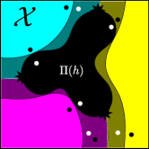
Figure 1: A depiction of a holomorphic classifier $h$ with three classes and its analytic polyhedra $\Pi(h)$. The shaded region represents the margin of the classifier and the dashed lines show the geometrical position of the decision boundary. The white circles are adversarial examples and they are benign otherwise.

Finally, if the result of second experiment indicated that $\varepsilon>0$, we will try to measure the continuity bias for the family of binary classifiers that can be constructed by combining the classes of $S$. If the proposal is true, then we should observe that $\varepsilon>0$ for these classifiers.

We will make use of a method of statistical hypothesis testing[38, section 3.5] to show that $\varepsilon>0$. To measure $\varepsilon$, we will perform an experiment similar to what we described for holomorphic hypotheses. We will train three classifiers $h,f,g\in\mathcal{H}(\omega)$ on $S_{\mathrm{adv}}$, $S_{\mathrm{nat}}$ and $S$ respectively, and then compute the gap between the loss of $g$ with the loss of a classifier that switches between $h$ and $f$. We will be using the same data sets that were generated for holomorphic hypotheses in the previous experiment.

To perform the test, we need to first choose a null $\mathbf{H_{0}}$ and an alternative $\mathbf{H_{1}}$ hypotheses. The aim of statistical hypothesis testing is to see if our observations provide enough evidence to accept $\mathbf{H_{1}}$. In our case, the null hypothesis is $\mathbf{H_{0}}:\varepsilon\leq 0$, and the alternative is $\mathbf{H_{1}}:\varepsilon>0$. Since we are testing the mean of the continuity bias, we can assume that the distribution of $\varepsilon$ is normal with some unknown mean and variance. To perform the test, we first need to compute the sample mean $\bar{\varepsilon}$ and the unbiased sample standard deviation $\sigma$, and then compute the test statistic

$$T=\frac{\bar{\varepsilon}}{\sigma}\sqrt{n},$$ (40)

in which $n$ is the size of the samples of $\varepsilon$. We then need to compare $T$ with the critical value

$$t=t_{\nu}^{-1}(1-c),$$ (41)

in which $t_{\nu}^{-1}$ is the inverse cumulative distribution function of a t-student random variable with $\nu=n-1$ degrees of freedom, and $c\in(0,1)$ is the confidence level of the test. Finally, We will accept $\mathbf{H_{1}}$ if $T>t$ and reject it otherwise.

In the end, we further need to check whether the observed bias would vanish if the target of the learning rule is continuous. To this end, we will perform the same statistical hypothesis testing procedure, with the difference that we will perform the test for random regression, instead of classification, learning problems. We will choose the target of regression problems to be a random continuous function in $\mathcal{H}(\mathcal{X})$. Similar to before, we are interested in accepting or rejecting $\mathbf{H_{1}}$. However, we are expecting to reject $\mathbf{H_{1}}$ in this experiment. Of course, rejecting $\mathbf{H_{1}}$ does not mean that $\mathbf{H_{0}}$ is accepted.

IV Implementing weakly-harmonic classifiers

In this section we will focus on giving a more practical perspective on previous sections and describe the details of the representation that we will be using to conduct our experiments. While the features proposed in theorem II.5 are perfectly fine in lower dimensions, the dimensions of a typical learning problem is prohibitively large, and the count of the features would grow combinatorially with dimensions. A common solution to the issue of combinatorial explosion in machine learning is to assume independence between variables. These methods have been successfully applied to probabilistic graphical models in the past[39, chapter 10].

Here, we will adapt the strategy used by convolutional neural networks (CNN) to implement an image classifier. The idea is to use lemma II.6 and only compute features $\varphi_{\alpha}$ for pixels that are close together. The similarities between the representation of lemma II.6 and a neural network would allow us to reuse most of the infrastructure available to artificial neural networks. The same could be said of theorem II.8 as well.

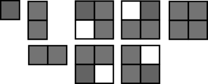
Figure 2: The templates that will be used in the experiments. These templates are chosen so that all overlapping templates of lower degree would take part in the model as well. The weight of the white pixels are 0 and otherwise they are 1.

The overall architecture of the implementation is similar to a standard CNN with a few differences. First, it does not actually go deep. In other words, every filter is convolved with the image and then directly fed to the single dense layer at the end. Second, the weights of the filters are not learned during training and are fixed before training starts. The reason is that $\alpha\in\mathbb{N}^{n}$ and we would need to incorporate mixed-integer programming to do so. Consequently, we will call them templates instead of filters to emphasize this distinction. Each template will be reused with up to 5 pixels of dilation so that the model is able to capture correlations between far away pixels as well.

Given that we are trying to learn a hypothesis with minimal Dirichlet energy, we should incorporate all overlapping templates $\beta$ with $\|\beta\|_{1}<\|\alpha\|_{1}$ if we were to use $\alpha$ in the model. Otherwise, the model might attend to $\alpha$, when in fact the correlation was due to $\beta$. For example, if we were to include $\cos(x_{1})\cos(x_{2})$, then we must include $\cos(x_{1})$ and $\cos(x_{2})$ as well to make sure that the hypothesis with the smallest Dirichlet energy is learned. Finally, we will only consider templates with $\|\alpha\|_{\infty}\leq 1$. We conjecture that features with $\|\alpha\|_{\infty}>1$ would not make any significant contribution to the model and will omit them. We emphasize that we will be using the weakly-harmonic features $\varphi^{*}$ in the model so that the implementation of weight decay in standard optimizers could be exploited to minimize the Dirichlet energy of the model. We have reported the templates that were used in the experiments in Figure 2.

For a complex-valued hypothesis, we will take the real part of the complex logarithm $\log z=\log|z|+i\angle z$ of $h(z)$ before handing it over to the softmax activation. As a result, softmax activated holomorphic classifiers with $m$ classes would have the form:

$$\mathbb{P}(\mathrm{class}=j|z)=\frac{|h_{j}(z)|}{\sum_{k=1}^{m}|h_{k}(z)|},\quad j=1,\cdots,m.$$ (42)

The final important part of the implementation is that we will attach a constant zero hypothesis to the classifier that other hypotheses have to beat before they get rewarded by the loss function during training. In other words, if there are 10 labels for the hypothesis to learn, we will add an extra label corresponding to $\Pi(h)$ and train the model as if there were 11 labels to learn. There is no need to add training samples for the extra label. The extra label is added to force the learning rule into finding a hypothesis that has pushed the natural samples outside its analytic polyhedra as much as possible.

We will be using a standard projected gradient decent[6] (PGD) attack to construct adversarial examples. The only difference with a standard PGD attack is that we will exploit the periodicity of the holomorphic and weakly-harmonic features in theorems II.5 and II.8 and project the adversarial example inside $[0,1]^{n}$ instead of clipping the pixel values. Informally, when the attack hits the boundary of the domain, a clipping strategy would drag the sample along the boundary instead of letting the example leave $[0,1]^{n}$. In contrast, our strategy would be better described as the trajectory of a particle that bounces off of the boundary of the domain without losing any momentum. In other words, the path that the attack takes to get to the adversarial example is in reality a smooth path that leaves $\mathcal{X}$. However, we can project the example back into $[0,1]^{n}$ by applying

$$\mathrm{proj}(x)= \begin{cases}\mathrm{p}_{1}(x)&x>1\\ x&0\leq x\leq 1\\ \mathrm{p}_{0}(x)&x<0\end{cases},$$ (43)

$$\mathrm{p}_{1}(x)= \begin{cases}\mathrm{fp}(x)&[x]\,\mathrm{even}\\ 1-\mathrm{fp}(x)&[x]\,\mathrm{odd}\end{cases},$$ (44)

$$\mathrm{p}_{0}(x)= \begin{cases}-\mathrm{fp}(x)&[x]\,\mathrm{even}\\ 1+\mathrm{fp}(x)&[x]\,\mathrm{odd}\end{cases},$$ (45)

$$\mathrm{fp}(x)= x-[x],$$ (46)

to each dimension of the generated adversarial example, and find a test sample inside $[0,1]^{n}$ for which $h$ would give the same prediction.

V Experiments

We have conducted three experiments in order to verify and test the proposal as described in section III. All three experiments were conducted on two datasets of the MNIST family; the MNIST dataset itself[40] and FashionMNIST[41]. The MNIST dataset contains $28\times 28$ gray-scale images of handwritten digits and FashionMNIST (FMNIST) is made of $28\times 28$ gray-scale images of everyday clothing items such as shirts and shoes. The loss function was the cross-entropy loss and the optimizer used in the experiments was an implementation of batch gradient decent that is provided by the PyTorch(2.1.0)[42] library. Each batch contained 32 training samples and we continued the training for 5 epochs. The learning rate of the optimizer was set to 0.001, the momentum was 0.9 and the weight decay was 1. All experiments were conducted on an Intel Core i5-6600K @ 3.5GHz, 8.00 GB of RAM and no GPUs. The implementation of the adversarial attack was provided by the CleverHans(4.0.0)[43] library. The attacks were constrained in a $\ell^{\infty}$-ball with a radius of 0.3 and performed 40 steps of projected gradient decent with step size of 0.01. The detection scores are computed with the help of the Scikit-learn(1.3.0)[44] library.

V-A Adversarial example detection

In this experiment, we test whether we can detect an adversarial example by checking to see if the examples falls inside the analytic polyhedra $\Pi(h)$ of the hypotheses. We have performed two versions of this experiment. In one of the experiments the attacker is aware that we want to capture the adversarial examples in $\Pi(h)$ and in the other experiment the attacker is not aware of this issue. We will perform each experiment 10 times and report the average of the scores.

The results of the experiments for the holomorphic hypotheses are reported in table I. We can see that the performance of $\Pi(h)$ is somewhat consistent across the attacks. The performance of the targeted attacks vary between different classes and targeted adversarial examples of some classes cannot be effectively detected in this manner. More importantly, false positives are rare as demonstrated by the precision scores. Thus, the evidence are in support of the proposition that $\Pi(h)$ is a subset of the adversarial region of $h$ and that adversarial examples of the holomorphic classifiers tend to populate $\Pi(h)$, which is the result that we were looking for.

TABLE I: The performance of the analytic polyhedra in detecting adversarial examples. The results are divided by the property whether the attacker is aware of the extra class or not. The target column specifies the target label of the targeted attack.

	FMNIST						MNIST
attack target	w/ extra			w/o extra			w/ extra			w/o extra
	precision	recall	F1	precision	recall	F1	precision	recall	F1	precision	recall	F1
untargeted	0.934	0.458	0.614	0.936	0.471	0.625	0.908	0.409	0.562	0.910	0.422	0.575
0, T-shirt/top	0.891	0.290	0.436	0.908	0.350	0.503	0.872	0.309	0.453	0.890	0.365	0.515
1, Trouser	0.897	0.309	0.458	0.909	0.357	0.512	0.906	0.454	0.603	0.913	0.493	0.638
2, Pullover	0.897	0.305	0.453	0.910	0.357	0.511	0.855	0.280	0.421	0.867	0.310	0.455
3, Dress	0.839	0.183	0.298	0.884	0.256	0.395	0.865	0.293	0.434	0.874	0.319	0.464
4, Coat	0.861	0.218	0.345	0.896	0.298	0.445	0.874	0.321	0.467	0.890	0.370	0.520
5, Sandal	0.849	0.193	0.313	0.858	0.217	0.345	0.869	0.309	0.453	0.885	0.351	0.501
6, Shirt	0.849	0.194	0.314	0.869	0.230	0.362	0.873	0.308	0.452	0.888	0.359	0.508
7, Sneaker	0.883	0.261	0.401	0.903	0.323	0.474	0.691	0.109	0.185	0.771	0.158	0.257
8, Bag	0.852	0.202	0.324	0.897	0.303	0.451	0.828	0.227	0.354	0.841	0.241	0.372
9, Ankle boot	0.904	0.327	0.479	0.918	0.385	0.540	0.863	0.285	0.425	0.881	0.337	0.485

V-B Infeasibility of holomorphic classifiers

We trained two more holomorphic classifiers for each learning problem. A classifier $f$ that is trained on $S_{\mathrm{adv}}$ and another classifier $g$ that is trained on $S$. We then compared the accuracy of the three classifiers on a test set consisting of unseen adversarial and benign samples. The results are reported in table II. We can see that the evidence points to the fact that the robust and accurate holomorphic classifier could be constructed by patching together $h$ and $f$, but not with a single holomorphic hypothesis $g$.

TABLE II: The accuracy of holomorphic classifiers on adversarial $S_{\mathrm{adv}}$ and benign $S_{\mathrm{nat}}$ test samples. $h$ is the original holomorphic hypothesis that is trained on $S_{\mathrm{nat}}$, $f$ is the one that is trained on $S_{\mathrm{adv}}$ and $g$ is the classifier that is trained on both training sets.

	FMNIST		MNIST
target	adversarial	benign	adversarial	benign
$h$	0.000	0.755	0.000	0.890
$f$	0.752	0.361	0.900	0.302
$g$	0.741	0.728	0.880	0.886

V-C Measuring the continuity bias

We are aiming to empirically reject the hypothesis that $\varepsilon\leq 0$. We will reuse the training sets that we gathered in the previous experiment $S_{\mathrm{adv}}$, $S_{\mathrm{nat}}$ and $S$. In this experiment we will be using the real-valued weakly-harmonic hypothesis space to measure $\varepsilon$.

We repeated the tests 20 times and computed the mean and standard deviation of the sampled continuity biases. Finally, we calculated the required test statistic and compared it to the corresponding critical value with the confidence level of 0.01. The results of the tests is reported in Table III. The results in case of discontinuous targets shows that we can accept $H_{1}$ with a very high confidence. $\mathbf{H_{1}}$ is rejected in case of continuous targets as predicted.

TABLE III: Results of the statistical hypothesis testing of $\varepsilon>0$. The results show that $\varepsilon\leq 0$ cannot be rejected in case of the regression tasks. In classification tasks on the other hand, we can accept $\varepsilon>0$ with high confidence.

dataset	critical value	continuous target		discontinuous target
		test statistic	$\mathbf{H_{1}}$	test statistic	$\mathbf{H_{1}}$
MNIST	2.54	-0.81	rejected	7.71	accepted
FMNIST	2.54	0.05	rejected	6.44	accepted

VI Conclusion

In this paper, we studied the effects of discontinuities of the target of a machine learning problem on the output of learning algorithms. To the best of our knowledge, we are the first to present empirical evidence that it might be impossible to train a hypothesis that is simultaneously robust, accurate and continuous. A shortcoming of the experimental approach of our proposal is that it is hard to isolate the effects of the choices we made regarding the construction of the hypotheses. Consequently, we acknowledge that the question of continuity of the optimal robust hypothesis would remain open until a suitable proof is presented.

The proposal of Tsipras et al. assumes that the trade-off between accuracy and robustness in classification problems exists because robust and accurate hypotheses are not realizable[7]. In other words, they argue that the learning problem is constrained in such a way that does not allow for robust and accurate hypotheses. In contrast, our proposal does not impose any restrictions on the optimal hypothesis and we argue that the observation of the trade-off is a part of the approximation error of the learning algorithm that would vanish if we were to give up on the continuity of the hypotheses.

Ilyas et al. posit that vulnerable hypotheses are attending nonrobust features in the natural data that are useful in classifying benign samples, but are a hindrance to the robustness of the hypotheses[45]. We believe on the other hand that a better description is that useful features are only defined locally, and that hypotheses attend to these features because no alternatives exist that would perform as good as these features on benign samples.

Goodfellow et al. suggest that vulnerable artificial neural networks are converging to the optimal linear hypothesis[4]. In contrast, we picture the robust and accurate hypothesis as a collection of analytic functions that cannot be glued together in a way that the hypothesis remain PAC in its domain. In this light, we argue that vulnerable ANNs are converging to the best piecewise analytic hypothesis that is defined on the support of the distribution of natural samples.

In conclusion, our proposal offers a new trajectory in the construction and the analysis of robust machine learning models. Our treatment of holomorphic functions as a learnable hypothesis space suggests that there are venues in machine learning that can benefit from the methods of functional analysis of several complex variables. We are under the impression that holomorphic hypotheses would find wider applications in machine learning due to their desirable and unique characteristics.

[Proofs of the Theorems]

Theorem II.1

Proof.

Given that $h$ has a series representation, we can compute its Dirichlet energy by:

$$\int_{\mathcal{X}}\|\nabla h(x)\|^{2}\,\mathrm{d}V(x)= \int_{\mathcal{X}}w^{T}J_{\varphi}(x)J_{\varphi}(x)^{T}w\,\mathrm{d}V(x),$$ (47)

$$= w^{T}\int_{\mathcal{X}}J_{\varphi}(x)J_{\varphi}(x)^{T}\,\mathrm{d}V(x)w,$$ (48)

in which $J_{\varphi}(x)$ is the Jacobian matrix of $\{\varphi_{k}\}_{1}^{K}$. But we know that

$$\int_{\mathcal{X}}J_{\varphi}(x)J_{\varphi}(x)^{T}\,\mathrm{d}V(x)=\Sigma=I.$$ (49)

Thus, $E[h]=w^{T}w$. ∎

Theorem II.2

Proof.

$$\int_{\mathcal{X}}J_{\varphi^{*}}(x)J_{\varphi^{*}}(x)^{T}\,\mathrm{d}V(x)= \Sigma^{-\frac{1}{2}}\Sigma\Sigma^{-\frac{1}{2}},$$ (50)

$$= I,$$ (51)

in which $J_{\varphi^{*}}(x)$ is the Jacobian matrix of $\{\varphi_{k}^{*}\}_{1}^{K}$. ∎

Theorem II.3

Proof.

We begin by recalling the Lagrangian of a weakly-harmonic learning problem in equation 18,

$$\mathcal{L} =\frac{1}{2}E[h]+\mathbb{E}_{S}[\mathrm{loss}(x;h,t)],$$ (52)

$$=\int_{\mathcal{X}}\frac{1}{2}\|\nabla h(x)\|^{2}+s(x)\mathrm{loss}(x;h,t)\,\mathrm{d}V(x).$$ (53)

According to variational calculus, the solution $h$ to the program satisfies the Euler-Lagrange equation,

$$\frac{\delta\mathcal{L}}{\delta h}(x)-\sum_{\|\alpha\|_{1}=1}\frac{\partial}{\partial x^{\alpha}}\frac{\delta\mathcal{L}}{\delta h^{(\alpha)}}(x)=0,$$ (54)

in which $\frac{\delta\mathcal{L}}{\delta h^{(\alpha)}}$ is the variational derivative of $\mathcal{L}$ with respect to $h^{(\alpha)}$. Substituting the Lagrangian inside the Euler-Lagrange equation we would have:

$$\frac{\delta\mathcal{L}}{\delta h}(x) =s(x)\mathrm{loss}_{h}(x;h,t),$$ (55)

$$\frac{\delta\mathcal{L}}{\delta h^{(\alpha)}}(x) =h^{(\alpha)}\quad\|\alpha\|_{1}=1,$$ (56)

$$0 =s(x)\mathrm{loss}_{h}(x;h,t)-\Delta h(x).$$ (57)

∎

Theorem II.4

Proof.

We begin by first showing (2). Suppose that $\{\varphi_{k}\}_{1}^{\infty}$ is the set of eigenfunctions of the Laplacian operator with eigenvalues $\{\lambda_{k}\}_{1}^{\infty}$ and some function $u\in\mathcal{H}(\mathcal{X})$. Then the Green function $G(x,x^{\prime})$ satisfies the following PDE:

$$\Delta G(x,x^{\prime}) =-\delta\big{(}\|x-x^{\prime}\|\big{)},$$ (58)

$$\frac{\partial G}{\partial\hat{n}}(x,x^{\prime}) =0\quad x\in\partial\mathcal{X},$$ (59)

in which $\delta(\cdot)$ is the Dirac’s delta. Since $\{\varphi_{k}\}_{1}^{\infty}$ are the results of separation of variables, we can assume that $G(x,x^{\prime})$ has a series representation:

$$G(x,x^{\prime})=\sum_{k=1}^{\infty}\frac{\varphi_{k}(x)\varphi_{k}(x^{\prime})}{\lambda_{k}^{2}}.$$ (60)

We can now use the divergence theorem to get

$$\int_{\mathcal{X}}\nabla\cdot\big{(}u\nabla G(x^{\prime})\big{)}\,\mathrm{d}V(x) =\int_{\partial\mathcal{X}}u\frac{\partial G(x^{\prime})}{\partial\hat{n}}\,\mathrm{d}A(x),$$ (61)

$$\int_{\mathcal{X}}\nabla\cdot\big{(}G(x^{\prime})\nabla u\big{)}\,\mathrm{d}V(x) =\int_{\partial\mathcal{X}}G(x^{\prime})\frac{\partial u}{\partial\hat{n}}\,\mathrm{d}A(x),$$ (62)

in which we have omitted the dependence of functions on $x$ for brevity, and then apply the chain rule of divergence:

$$\nabla\cdot\big{(}u\nabla G(x^{\prime})\big{)} =\nabla u\cdot\nabla G(x^{\prime})+u\Delta G(x^{\prime}),$$ (63)

$$\nabla\cdot\big{(}G(x^{\prime})\nabla u\big{)} =\nabla u\cdot\nabla G(x^{\prime})+G(x^{\prime})\Delta u,$$ (64)

and substitute the PDE definitions of $G(x^{\prime})$ and $u$ to get

$$u(x^{\prime})=\int_{\partial\mathcal{X}}G(x^{\prime})g\,\mathrm{d}A(x)-\int_{\mathcal{X}}G(x^{\prime})f\,\mathrm{d}V(x).$$ (65)

Thus, $u$ has a series representation in $\{\varphi_{k}\}_{1}^{\infty}$.

Having proved (2), it is easy to show (1) as $\mathcal{H}(\mathcal{X})$ can be exhausted by a countable increasing union of PAC learnable hypothesis spaces[31, theorem 7.2]:

$$\mathcal{H}(\mathcal{X})=\bigcup_{K=1}^{\infty}\Big{\{}h\in H^{2}(\mathcal{X})\,|\,h=b+\sum_{k=1}^{K}w_{k}\varphi_{k}\Big{\}}.$$ (66)

Finally, we can compute the tuning matrix of $\{\varphi_{k}\}_{1}^{\infty}$ with the help of the PDE definition of $\varphi_{k}$, the divergence theorem and the chain rule of divergence to get

$$\int_{\mathcal{X}}\nabla\varphi_{k}\cdot\nabla\varphi_{l}\,\mathrm{d}V(x) =\lambda_{k}^{2}\int_{\mathcal{X}}\varphi_{k}\varphi_{l}\,\mathrm{d}V(x),$$ (67)

$$=\lambda_{l}^{2}\int_{\mathcal{X}}\varphi_{k}\varphi_{l}\,\mathrm{d}V(x).$$ (68)

Thus it must be that $\Sigma_{kl}=0$ when $\lambda_{k}\neq\lambda_{l}$. Moreover, in case $\lambda_{k}=\lambda_{l}$, $\Sigma_{kl}$ would again be zero when $\varphi_{k}$ and $\varphi_{l}$ differ in a separated eigenfunction because eigenfunctions of the resulting Sturm-Liouville ordinary differential equations are orthogonal. Consequently $\Sigma$ is diagonal and (3) is proven. ∎

Theorem II.5

Proof.

We begin by assuming that any eigenfunction can be separated in $x$,

$$\varphi_{\alpha}(x)=\prod_{j=1}^{n}\Phi(x_{j};\alpha_{j}).$$ (69)

Thus,

$$\Delta\varphi_{\alpha}(x) =-\lambda_{\alpha}^{2}\varphi_{\alpha}(x),$$ (70)

$$\varphi_{\alpha}(x)\sum_{j=1}^{n}\frac{\Phi^{(2)}(x_{j};\alpha_{j})}{\Phi(x_{j};\alpha_{j})} =-\lambda_{\alpha}^{2}\varphi_{\alpha}(x),$$ (71)

$$\sum_{j=1}^{n}\frac{\Phi^{(2)}(x_{j};\alpha_{j})}{\Phi(x_{j};\alpha_{j})} =-\lambda_{\alpha}^{2}.$$ (72)

Now we can separate the variables and reach the Sturm-Liouville ordinary differential equations

$$\Phi^{(2)}(x_{j};\alpha_{j})+\alpha_{j}^{2}\Phi(x_{j};\alpha_{j}) =0,\quad\|\alpha\|_{2}^{2}=\lambda_{\alpha}^{2},$$ (73)

$$\Phi^{(1)}(0;\alpha_{j})=\Phi^{(1)}(\pi;\alpha_{j}) =0.$$ (74)

Then,

$$\Phi(x_{j};\alpha_{j})=c_{1}\cos(\alpha_{j}x_{j})+c_{2}\sin(\alpha_{j}x_{j}).$$ (75)

However, given the boundary condition we can see that $c_{2}=0$.

The corresponding diagonal element of $\Sigma$ is:

$$\Sigma_{jj} =\|\alpha_{j}\|_{2}^{2}\int_{\omega}|\varphi_{j}(x)|^{2}\,\mathrm{d}V(x),$$ (76)

$$=\|\alpha_{j}\|_{2}^{2}\int_{\omega}\prod_{l=1}^{n}\cos^{2}(\alpha_{jl}x_{l})\,\mathrm{d}V(x),$$ (77)

$$=\frac{\pi^{n}}{2^{n}}\|\alpha_{j}\|_{2}^{2}.$$ (78)

After scaling $\Sigma$ with $\frac{2^{n}}{\pi^{n}}$, the proof is complete. ∎

Lemma II.6

Proof.

Consider the product to sum formula of cosines,

$$\cos(x_{j})\cos(x_{k})=\frac{1}{2}\big{(}\cos(x_{j}+x_{k})+\cos(x_{j}-x_{k})\big{)}.$$ (79)

Thus, we can transform $\varphi_{\alpha}$ by repeated application of the product to some formula to a summation of $2^{n-1}$ cosine functions,

$$\prod_{j=1}^{n}\cos(\alpha_{j}x_{j})=\frac{1}{2^{n-1}}\big{(}\cos(\alpha_{1}x_{1}+\cdots+\alpha_{n}x_{n})+\cdots\\ +\cos(\alpha_{1}x_{1}-\cdots-\alpha_{n}x_{n})\big{)}.$$ (80)

To make the expression invariant to the choice of the starting index, we exploit the evenness of the cosine function and add $2^{n-1}$ more equal cosine functions with negated inputs to the expression to get to the theorem. We should emphasize that there is no need to compute all $2^{n}$ terms because $\cos(\alpha_{j}x_{j})=1$ when $\alpha_{j}=0$ and $\alpha$ is sparse in practice. ∎

Theorem II.7

Proof.

We will continue from where we left off in the proof of theorem II.5. Now that we have an extra dimension for every real dimension, we only have to separate each $\Phi$ again between $x_{j}$ and $y_{j}$,

$$\Psi(x_{j},y_{j};\alpha_{j})=\Phi(x_{j};\alpha_{j})\Theta(y_{j};\alpha_{j}),$$ (81)

and then solve for $\Delta\Psi(x_{j},y_{j};\alpha_{j})=0$. Consequently,

$$\Theta(y_{j};\alpha_{j})=c_{1}\cosh(\alpha_{j}y_{j})+c_{2}\sinh(\alpha_{j}y_{j}).$$ (82)

Assuming $\frac{\partial\Theta}{\partial y_{j}}(0)=0$, we can see that $c_{2}=0$. However, another function $\Psi^{\dagger}$ exists for which $\Psi^{\dagger}(x_{j},0;\alpha_{j})=0$,

$$\Psi^{\dagger}(x_{j},y_{j};\alpha_{j})=\sin(\alpha_{j}x_{j})\sinh(\alpha_{j}y_{j}),$$ (83)

called the conjugate harmonic of $\Psi(x_{j},y_{j};\alpha_{j})$ and we have

$$\cos(\alpha_{j}z_{j})=\Psi(x_{j},y_{j};\alpha_{j})+i\Psi^{\dagger}(x_{j},y_{j};\alpha_{j}),$$ (84)

which satisfies the Cauchy-Riemann equations and thus is holomorphic. ∎

Theorem II.8

Proof.

The first part of the theorem is a direct consequence of the existence of a biholomorphic map between $U_{\omega}$ and $D^{n}(0,1)$ and the fact that $z^{\alpha}$ is an orthogonal set of basis functions for the intersection of $\mathcal{O}(D^{n}(0,1))$ and $L^{2}(D^{n}(0,1))$, which is a Hilbert space called the Bergman space $A^{2}(D^{n}(0,1))$ of the poly-disk[33, p. 60]. The inner product of $A^{2}$ uses the usual inner product of $\mathbb{C}^{n}$ which conjugates the left side of the inner product:

$$z_{1}\cdot z_{2}=z_{1}^{H}z_{2}.$$ (85)

We can compute $\Sigma_{kl}$ as:

$$\Sigma_{kl} =\int_{\omega}\nabla\psi_{\alpha_{k}}(x)\cdot\nabla\psi_{\alpha_{l}}(x)\,\mathrm{d}V(x),$$ (86)

$$=\alpha_{k}\cdot\alpha_{l}\int_{\omega}e^{i(\alpha_{l}-\alpha_{k})\cdot x}\,\mathrm{d}V(x),$$ (87)

$$=\begin{cases}(2\pi)^{n}\|\alpha_{k}\|_{2}^{2}&\quad k=l\\ 0&\quad\mathrm{o.w.}\end{cases}.$$ (88)

We then scale $\Sigma$ with $(2\pi)^{-n}$ and the theorem follows. ∎

Theorem III.1

Proof.

We will proceed by turning the smoothing problems into Cousin problems[33, chapter 6].

Consider the first smoothing problem, and define functions $g_{lk}:\Omega_{k}\cap\Omega_{l}\to\mathbb{C}$ such that

$$g_{kl}(z)=g_{l}(z)-g_{k}(z)\quad z\in\Omega_{k}\cap\Omega_{l}.$$ (89)

It can be checked that

$$g_{kl}(z)+g_{lk}(z) =0\quad z\in\Omega_{k}\cap\Omega_{l},$$ (90)

$$g_{jk}(z)+g_{kl}(z)+g_{lj}(z) =0\quad z\in\Omega_{j}\cap\Omega_{k}\cap\Omega_{l}.$$ (91)

Thus $\{g_{kl}\}_{k,l=1}^{K}$ is valid for a first Cousin problem[33, page 247]. The first Cousin problem is always solvable by continuous functions[33, proposition 6.1.7]. Furthermore, if $\Omega$ is a domain of holomorphy, the first Cousin problem is also solvable by holomorphic functions[33, proposition 6.1.8]. This will conclude the proof of the first part of the theorem.

Now consider the second smoothing problem, and define functions $g_{lk}:\Omega_{k}\cap\Omega_{l}\to\mathbb{C}$ such that

$$g_{kl}(z)=\frac{g_{l}(z)}{g_{k}(z)}\quad z\in\Omega_{k}\cap\Omega_{l}.$$ (92)

It can be checked that

$$g_{kl}(z)g_{lk}(z) =1\quad z\in\Omega_{k}\cap\Omega_{l},$$ (93)

$$g_{jk}(z)g_{kl}(z)g_{lj}(z) =1\quad z\in\Omega_{j}\cap\Omega_{k}\cap\Omega_{l}.$$ (94)

Thus $\{g_{kl}\}_{k,l=1}^{K}$ is valid for a second Cousin problem[33, page 247]. The second Cousin problem can be solved by holomorphic functions on $\Omega$ if and only if it can be solved just continuously[33, proposition 6.1.11]. ∎

Theorem III.2

Proof.

Consider a PAC covering $\{(h_{k},\omega_{k})\}_{k=1}^{\infty}$ of $\mathcal{X}$ in which $\omega_{k}\subset\mathbb{R}^{n}$ is an open hypercube, $h_{k}\in\mathcal{H}(\omega_{k})$, and $\mathbf{V}(h_{k})\cap\omega_{l}=\mathbf{V}(h_{l})\cap\omega_{k}$. Theorem II.4 states that $h_{k}$ has a series representation in eigenfunctions of $\mathcal{H}(\omega_{k})$, and according to theorems II.5 and II.7 $h_{k}$ can be holomorphically extended to the tube domain $T_{\omega_{k}}$. Since $\Im[h_{k}(z)]=0$ and $\frac{\partial\Re[h_{k}]}{\partial y_{j}}(z)=0,j=1,\cdots,n$ for $z\in\omega_{k}$, then some $\Omega_{k}\subset T_{\omega_{k}}$ exists for which $\Re[h_{k}(z)]$ is PAC on $\Omega_{k}$. Thus $\{(h_{k},\Omega_{k})\}_{k=1}^{K}$ is a holomorphic PAC covering of $\mathcal{X}$. We will denote $\Omega=\bigcup_{k=1}^{K}\Omega_{k}$. Since $\mathcal{X}$ is compact, we can choose a finite holomorphic PAC covering $\{(h_{k},\Omega_{k})\}_{k=1}^{K}$ of $\mathcal{X}$.

First, suppose that some real-valued $h_{c}\in C(\mathcal{X})$ exists that is PAC on $\mathcal{X}$. Then a continuous PAC extension of $h_{c}$ to $\Omega$ exists that is real on $\Omega\cap\mathbb{R}^{n}$, and nonvanishing outside of $\mathcal{X}$. Denote the decision boundary of $h_{c}$ by $M=\{z\in\Omega\,\|\,h_{c}(z)=0\}$. Then a choice of a PAC covering $\{(h_{k},\Omega_{k})\}_{k=1}^{K}$ of $\mathcal{X}$ exists that is valid for a smoothing problem, and the second smoothing problem of $\{(h_{k},\Omega_{k})\}_{k=1}^{K}$ is feasible by choosing $g^{\prime}_{k}(z)=\frac{h_{k}(z)}{h_{c}(z)}$. According to theorem III.1, a holomorphic solution $\{g_{k}(z)\}_{k=1}^{K}$ exists as well, and denote the smoothed holomorphic function by $h_{o}$. Since $g_{k}$ is nonvanishing, then $\mathbf{V}(h_{o})=M$.

Now assume that some $h_{o}\in\mathcal{O}(\Omega)$ exists for which $M=\mathbf{V}(h_{o})$ is the geometrical position of a PAC decision boundary. Then $\{g_{k}(z)\}_{k=1}^{K}$ is a holomorphic solution for the corresponding second smoothing problem of $\{(h_{k},\Omega_{k})\}_{k=1}^{K}$ for which $g_{k}(z)=\frac{h_{k}(z)}{h_{o}(z)}$ . Consequently, a continuous classifier $h_{c}\in C(\Omega)$ exists for which $\{z\in\Omega\,\|\,h_{c}(z)=0\}=M$, and $h_{c}$ is PAC on $\mathcal{X}$. ∎

References

- [1] Y. Liu, X. Chen, C. Liu, and D. Song, “Delving into transferable adversarial examples and black-box attacks,” in International Conference on Learning Representations, 2017. [Online]. Available: https://openreview.net/forum?id=Sys6GJqxl
- [2] C.-S. Lin, C.-Y. Hsu, P.-Y. Chen, and C.-M. Yu, “Real-world adversarial examples via makeup,” in ICASSP 2022 - 2022 IEEE International Conference on Acoustics, Speech and Signal Processing (ICASSP), 2022, pp. 2854–2858.
- [3] C. Szegedy, W. Zaremba, I. Sutskever, J. Bruna, D. Erhan, I. J. Goodfellow, and R. Fergus, “Intriguing properties of neural networks,” in 2nd International Conference on Learning Representations, ICLR 2014, Banff, AB, Canada, April 14-16, 2014, Conference Track Proceedings, Y. Bengio and Y. LeCun, Eds., 2014.
- [4] I. J. Goodfellow, J. Shlens, and C. Szegedy, “Explaining and harnessing adversarial examples,” in 3rd International Conference on Learning Representations, ICLR 2015, San Diego, CA, USA, May 7-9, 2015, Conference Track Proceedings, Y. Bengio and Y. LeCun, Eds., 2015.
- [5] T. Bai, J. Luo, J. Zhao, B. Wen, and Q. Wang, “Recent advances in adversarial training for adversarial robustness,” in Proceedings of the Thirtieth International Joint Conference on Artificial Intelligence, IJCAI-21, Z.-H. Zhou, Ed. International Joint Conferences on Artificial Intelligence Organization, 8 2021, pp. 4312–4321, survey Track. [Online]. Available: https://doi.org/10.24963/ijcai.2021/591
- [6] A. Madry, A. Makelov, L. Schmidt, D. Tsipras, and A. Vladu, “Towards deep learning models resistant to adversarial attacks,” in International Conference on Learning Representations, 2018.
- [7] D. Tsipras, S. Santurkar, L. Engstrom, A. Turner, and A. Madry, “Robustness may be at odds with accuracy,” in International Conference on Learning Representations, 2019.
- [8] D. Su, H. Zhang, H. Chen, J. Yi, P.-Y. Chen, and Y. Gao, “Is robustness the cost of accuracy? – a comprehensive study on the robustness of 18 deep image classification models,” in Computer Vision – ECCV 2018, V. Ferrari, M. Hebert, C. Sminchisescu, and Y. Weiss, Eds. Cham: Springer International Publishing, 2018, pp. 644–661.
- [9] Y.-Y. Yang, C. Rashtchian, H. Zhang, R. R. Salakhutdinov, and K. Chaudhuri, “A closer look at accuracy vs. robustness,” in Advances in Neural Information Processing Systems, H. Larochelle, M. Ranzato, R. Hadsell, M. Balcan, and H. Lin, Eds., vol. 33. Curran Associates, Inc., 2020, pp. 8588–8601. [Online]. Available: https://proceedings.neurips.cc/paper_files/paper/2020/file/61d77652c97ef636343742fc3dcf3ba9-Paper.pdf
- [10] T. Tanay and L. D. Griffin, “A boundary tilting persepective on the phenomenon of adversarial examples,” CoRR, vol. abs/1608.07690, 2016. [Online]. Available: http://arxiv.org/abs/1608.07690
- [11] D. Kang, Y. Sun, T. Brown, D. Hendrycks, and J. Steinhardt, “Transfer of adversarial robustness between perturbation types,” 2019.
- [12] P. Maini, E. Wong, and J. Z. Kolter, “Adversarial robustness against the union of multiple perturbation models,” in Proceedings of the 37th International Conference on Machine Learning, ser. ICML’20. JMLR.org, 2020.
- [13] M. Cisse, P. Bojanowski, E. Grave, Y. Dauphin, and N. Usunier, “Parseval networks: Improving robustness to adversarial examples,” in Proceedings of the 34th International Conference on Machine Learning, ser. Proceedings of Machine Learning Research, D. Precup and Y. W. Teh, Eds., vol. 70. PMLR, 06–11 Aug 2017, pp. 854–863.
- [14] T. Huster, C.-Y. J. Chiang, and R. Chadha, “Limitations of the lipschitz constant as a defense against adversarial examples,” in ECML PKDD 2018 Workshops, C. Alzate, A. Monreale, H. Assem, A. Bifet, T. S. Buda, B. Caglayan, B. Drury, E. García-Martín, R. Gavaldà, I. Koprinska, S. Kramer, N. Lavesson, M. Madden, I. Molloy, M.-I. Nicolae, and M. Sinn, Eds. Cham: Springer International Publishing, 2019, pp. 16–29.
- [15] A. Fan, X. Jiang, Y. Ma, X. Mei, and J. Ma, “Smoothness-driven consensus based on compact representation for robust feature matching,” IEEE Transactions on Neural Networks and Learning Systems, vol. 34, no. 8, pp. 4460–4472, 2023.
- [16] A. Raghunathan*, S. M. Xie*, F. Yang, J. Duchi, and P. Liang, “Adversarial training can hurt generalization,” in ICML 2019 Workshop on Identifying and Understanding Deep Learning Phenomena, 2019. [Online]. Available: https://openreview.net/forum?id=SyxM3J256E
- [17] C. Buckner, “Understanding adversarial examples requires a theory of artefacts for deep learning,” Nature Machine Intelligence, vol. 2, pp. 731–736, 12 2020.
- [18] C. Lyu, K. Huang, and H.-N. Liang, “A unified gradient regularization family for adversarial examples,” in 2015 IEEE International Conference on Data Mining, 2015, pp. 301–309.
- [19] D. V. oraz Adrián Csiszárik oraz Zsolt Zombori, “Gradient regularization improves accuracy of discriminative models,” Schedae Informaticae, vol. 2018, no. Volume 27, 2018. [Online]. Available: https://www.ejournals.eu/Schedae-Informaticae/2018/Volume-27/art/13926/
- [20] D. Barrett and B. Dherin, “Implicit gradient regularization,” in International Conference on Learning Representations, 2021. [Online]. Available: https://openreview.net/forum?id=3q5IqUrkcF
- [21] D. Liu, L. Y. Wu, B. Li, F. Boussaid, M. Bennamoun, X. Xie, and C. Liang, “Jacobian norm with selective input gradient regularization for interpretable adversarial defense,” Pattern Recognition, vol. 145, p. 109902, 2024. [Online]. Available: https://www.sciencedirect.com/science/article/pii/S0031320323006003
- [22] A. Ross and F. Doshi-Velez, “Improving the adversarial robustness and interpretability of deep neural networks by regularizing their input gradients,” Proceedings of the AAAI Conference on Artificial Intelligence, vol. 32, no. 1, Apr. 2018.
- [23] S. Lee, H. Kim, and J. Lee, “Graddiv: Adversarial robustness of randomized neural networks via gradient diversity regularization,” IEEE Transactions on Pattern Analysis and Machine Intelligence, vol. 45, no. 2, pp. 2645–2651, 2023.
- [24] G. Adam, P. Smirnov, B. Haibe-Kains, and A. Goldenberg, “Reducing adversarial example transferability using gradient regularization,” CoRR, vol. abs/1904.07980, 2019. [Online]. Available: http://arxiv.org/abs/1904.07980
- [25] N. Carlini and D. Wagner, “Adversarial examples are not easily detected: Bypassing ten detection methods,” in Proceedings of the 10th ACM Workshop on Artificial Intelligence and Security, ser. AISec ’17. New York, NY, USA: Association for Computing Machinery, 2017, p. 3–14.
- [26] A. Aldahdooh, W. Hamidouche, S. A. Fezza, and O. Déforges, “Adversarial example detection for dnn models: A review and experimental comparison,” Artificial Intelligence Review, vol. 55, no. 6, pp. 4403–4462, 2022.
- [27] K. Grosse, P. Manoharan, N. Papernot, M. Backes, and P. McDaniel, “On the (Statistical) Detection of Adversarial Examples,” arXiv e-prints, p. arXiv:1702.06280, Feb. 2017.
- [28] X. Li and F. Li, “Adversarial examples detection in deep networks with convolutional filter statistics,” in Proceedings of the IEEE International Conference on Computer Vision (ICCV), Oct 2017.
- [29] S. Pertigkiozoglou and P. Maragos, “Detecting adversarial examples in convolutional neural networks,” 2018.
- [30] D. Hendrycks and K. Gimpel, “A baseline for detecting misclassified and out-of-distribution examples in neural networks,” in International Conference on Learning Representations, 2017. [Online]. Available: https://openreview.net/forum?id=Hkg4TI9xl
- [31] S. Shalev-Shwartz and S. Ben-David, Understanding Machine Learning: From Theory to Algorithms, ser. Understanding Machine Learning: From Theory to Algorithms. Cambridge University Press, 2014.
- [32] W. Rudin, Principles of Mathematical Analysis, ser. International series in pure and applied mathematics. McGraw-Hill, 1976.
- [33] S. Krantz, Function Theory of Several Complex Variables, ser. AMS Chelsea Publishing Series. American Mathematical Society, 2001.
- [34] A. Monna, Dirichlet’s Principle: A Mathematical Comedy of Errors and Its Influence on the Development of Analysis. Oosthoek, Scheltema & Holkema, 1975.
- [35] D. Gilbarg and N. Trudinger, Elliptic Partial Differential Equations of Second Order, ser. Classics in Mathematics. Springer Berlin Heidelberg, 2001.
- [36] E. Stein and R. Shakarchi, Real Analysis: Measure Theory, Integration, and Hilbert Spaces. Princeton University Press, 2009.
- [37] S. G. Krantz, “On limits of sequences of holomorphic functions,” Rocky Mountain Journal of Mathematics, vol. 43, pp. 273–283, 2010.
- [38] E. L. Lehmann and J. P. Romano, Testing statistical hypotheses, 3rd ed., ser. Springer Texts in Statistics. New York: Springer, 2005.
- [39] C. Bishop, Pattern Recognition and Machine Learning. Springer, January 2006.
- [40] Y. LeCun and C. Cortes, “MNIST handwritten digit database,” 2010.
- [41] H. Xiao, K. Rasul, and R. Vollgraf, “Fashion-mnist: a novel image dataset for benchmarking machine learning algorithms,” 2017, cite arxiv:1708.07747Comment: Dataset is freely available at https://github.com/zalandoresearch/fashion-mnist Benchmark is available at http://fashion-mnist.s3-website.eu-central-1.amazonaws.com/.
- [42] A. Paszke, S. Gross, F. Massa, A. Lerer, J. Bradbury, G. Chanan, T. Killeen, Z. Lin, N. Gimelshein, L. Antiga, A. Desmaison, A. Kopf, E. Yang, Z. DeVito, M. Raison, A. Tejani, S. Chilamkurthy, B. Steiner, L. Fang, J. Bai, and S. Chintala, “Pytorch: An imperative style, high-performance deep learning library,” in Advances in Neural Information Processing Systems 32. Curran Associates, Inc., 2019, pp. 8024–8035.
- [43] N. Papernot, F. Faghri, N. Carlini, I. Goodfellow, R. Feinman, A. Kurakin, C. Xie, Y. Sharma, T. Brown, A. Roy, A. Matyasko, V. Behzadan, K. Hambardzumyan, Z. Zhang, Y.-L. Juang, Z. Li, R. Sheatsley, A. Garg, J. Uesato, W. Gierke, Y. Dong, D. Berthelot, P. Hendricks, J. Rauber, and R. Long, “Technical report on the cleverhans v2.1.0 adversarial examples library,” arXiv preprint arXiv:1610.00768, 2018.
- [44] F. Pedregosa, G. Varoquaux, A. Gramfort, V. Michel, B. Thirion, O. Grisel, M. Blondel, P. Prettenhofer, R. Weiss, V. Dubourg, J. Vanderplas, A. Passos, D. Cournapeau, M. Brucher, M. Perrot, and E. Duchesnay, “Scikit-learn: Machine learning in Python,” Journal of Machine Learning Research, vol. 12, pp. 2825–2830, 2011.
- [45] A. Ilyas, S. Santurkar, D. Tsipras, L. Engstrom, B. Tran, and A. Madry, “Adversarial examples are not bugs, they are features,” in Advances in Neural Information Processing Systems 32: Annual Conference on Neural Information Processing Systems 2019, NeurIPS 2019, December 8-14, 2019, Vancouver, BC, Canada, H. M. Wallach, H. Larochelle, A. Beygelzimer, F. d’Alché-Buc, E. B. Fox, and R. Garnett, Eds., 2019, pp. 125–136.