Effective action and black hole solutions in asymptotically safe quantum gravity

Abstract

We derive the quantum effective action and the respective quantum equations of motion from multi-graviton correlation functions in asymptotically safe quantum gravity. The fully momentum-dependent couplings of three- and four-graviton scatterings are computed within the functional renormalisation group approach and the effective action is reconstructed from these vertices. The resulting quantum equations of motion are solved numerically for quantum black hole geometries. Importantly, the black hole solutions show signatures of quantum gravity outside the classical horizon, which manifest in the behaviour of the temporal and radial components of the metric. Three different types of solutions with distinct causal structures are identified and the phase structure of the solution space is investigated.

I Introduction

Observable signatures of quantum gravity are very elusive due to their natural (trans-) Planckian scales. A potential exception is the physics of black holes. While curvatures outside the horizon of a classical black hole are typically below the Planck scale, the consistent description of these spacetimes in terms of solutions of the quantum equation of motion may still contain traces of quantum gravity in the geometry outside the horizon.

In the present work we investigate this intriguing scenario within asymptotically safe gravity [1], where the gravitational interaction approaches an interacting ultraviolet fixed point at trans-Planckian scales. In the past three decades this quantum field theoretical closure of gravity has been established as a serious contenter for a consistent quantum theory of gravity within the functional renormalisation group (fRG) approach, starting with the seminal paper of Reuter in [2]. For recent reviews see [3, 4, 5, 6].

The fRG can be used for computing the momentum-dependent correlation functions of $n$-graviton scatterings, which constitute the expansion coefficients of the effective action of asymptotically safe gravity in an expansion in powers of fluctuating gravitons on a flat background. This fluctuation approach has been set up in [7], and has been worked out further in [8, 9, 10, 11] for pure gravity, for reviews see [12, 6]. The respective correlation functions allow us to reconstruct the diffeomorphism-invariant effective action in terms of curvature invariants and covariant momentum dependences. The quantum equations of motion derived from the effective action can be solved for quantum black hole solutions whose geometries outside the horizon are then compared with their classical counterparts in a quest for signatures of quantum gravity.

In Section II we briefly introduce our setup. In particular, we introduce the quantum effective action for gravity in Section II.1, and discuss how to reconstruct the contributions of different curvature invariants in terms of momentum-dependent graviton correlation functions in Section II.2 and Section II.3. In Section III we introduce the functional renormalisation group, and present the computation and results of fully momentum-dependent graviton correlation functions. We use this data to reconstruct the effective action in Section IV. In Section V we study quantum black hole solutions in our theory. We present the effective field equations, which are the quantum version of Einstein’s equations, in Section V.1. Spherically symmetric solutions to the field equations are discussed and classified in Section V.2. We close with a brief summary in Section VI.

II Reconstructing the effective action

In this section we discuss the reconstruction of the diffeomorphism-invariant quantum effective action $\Gamma[g_{\mu\nu}]$. This is done by first reconstructing the Euclidean effective action from the correlation functions of the graviton, see e.g. [10, 13]. To this end, the effective action is expanded in powers of the curvature up to second order, while retaining the full covariant momentum dependence of the respective terms, that is the dependence on the Euclidean Laplace-Beltrami operator. Finally, we perform a Wick rotation of the Euclidean effective action.

II.1 The effective action

Euclidean gravity is described by the Wick-rotated Einstein-Hilbert action for the metric field $g_{\mu\nu}$,

$$S_{\text{EH}}[g_{\mu\nu}]=\frac{1}{16\pi G_{N}}\int_{x}\sqrt{g}\bigl{(}R-2\Lambda\bigr{)}\,,$$ (1)

where $g\coloneqq\det g_{\mu\nu}$, $R$ is the Ricci or curvature scalar, $\Lambda$ denotes the cosmological constant and $G_{N}=1/M_{\text{pl}}^{2}$ is the Newton constant related to the Planck mass $M_{\text{pl}}$. Equation 7 is endowed with a de-Donder-type gauge fixing, see Appendix A.

The quantum counter part of the classical action 1 is the quantum effective action $\Gamma[\bar{g},h]$, and the solution of the equations of motion derived from $\Gamma[\bar{g},h]$ governs the full quantum physics.

In $\Gamma[\bar{g},h]$, the full metric $g_{\mu\nu}$ is split into a background metric $\bar{g}_{\mu\nu}$ and dynamical fluctuations $h_{\mu\nu}$,

$$g_{\mu\nu}=\bar{g}_{\mu\nu}+\sqrt{Z_{h}\,G}\,h_{\mu\nu}\,,$$ (2)

where $Z^{1/2}_{h}$ is the wave function of the transverse-traceless (tt) mode $h_{tt}$ of the fluctuation field $h_{\mu\nu}$. This wave function captures the anomalous scaling of $h_{tt}$ relative to that of the background metric. The dimensional factor $G^{1/2}$ with momentum dimension $[G]=-2$ is related to the Newton constant and leads to the canonical dimension $[h_{\mu\nu}]=1$ of the fluctuation field. In classical gravity we choose $Z_{h}=1$ and $G=G_{N}$. Accordingly, the $n^{\text{th}}$-order fluctuation vertices are proportional to $G_{N}^{(n-2)/2}$.

We also remark that the wave functions of the different graviton modes, the transverse-traceless, the vector and scalar modes, are different from each other, as they receive different quantum corrections. Hence, it might be advantageous to split the fluctuation term in 2 into a sum over all modes with roots of their respective wave functions. However, in the present approximation we shall assume the dominance of the transverse-traceless mode and assign its wave function and coupling factor also to the other modes, hence using a uniform $Z_{h}=Z_{h_{tt}}$.

Finally, it is convenient to use fully (covariant) momentum-dependent $Z_{h}$ and $G$. This choice eliminates respective factors in the relations between the background and fluctuation vertices, the Nielsen identities, which is discussed in detail in the following Section II.3. Accordingly, we consider

$$Z_{h}=Z_{h}(\Delta)\,,\quad G=G(\Delta)\,,$$ (3)

with

$$\Delta=-{g}^{\mu\nu}{\nabla}_{\mu}{\nabla}_{\nu}\,,$$ (4)

where we used the covariant derivative $\nabla_{\mu}$. In the present work, we expand the full effective action in powers of the curvature, that is about flat space. In flat Euclidean space with

$$g_{\mu\nu}=\eta_{\mu\nu}=\delta_{\mu\nu}\,,$$ (5)

the spectral values of the Laplace-Beltrami operator are simply given by the momenta squared, ${\Delta(\eta)\exp\{\textrm{i}px\}=p^{2}\exp\{\textrm{i}px\}}$.

The gauge fixing leads to rather complicated Slavnov-Taylor identities for the correlation functions of the dynamical fluctuation field. However, a diffeomorphism-invariant action is given by the background effective action, defined at vanishing fluctuation field,

$$\Gamma[g]=\Gamma[g,h=0]\,,$$ (6)

where the background field is identified with the full (mean) metric. It can be shown via the Nielsen identities that the diffeomorphism invariance of the background effective action 6 is the physical one [6]. The Nielsen identities also link background correlation functions to fluctuation field ones, and in the following we reconstruct the background effective action 6 from fluctuation correlation functions.

To that end, we employ a curvature expansion about a flat background and parametrise $\Gamma[{g}]$ with an ansatz of the form

$$\Gamma[g_{\mu\nu}]= \,\frac{1}{16\pi}\int_{x}\sqrt{g}\,\Biggl{\{}{\mathcal{R}}(\Delta,R)$$

$$\,+Rf_{R^{2}}(\Delta)R+R_{\mu\nu}f_{R_{\mu\nu}^{2}}(\Delta)R^{\mu\nu}\Biggr{\}}\,.$$ (7)

The two two-point correlation functions of the curvature scalar and Ricci tensor, $f_{R^{2}}(\Delta)$ and $f_{R_{\mu\nu}^{2}}(\Delta)$, represent generalised dispersions and are also called form factors. These correlation functions or form factors have been investigated in e.g. [10] and [14, 15, 16, 17, 18, 19, 20, 21, 22, 23], for a recent review see [24].

The first term ${\mathcal{R}}(\Delta,R)$ contains the (classical) linear curvature scalar term. This term could be absorbed into the second term with $f_{R^{2}}(\Delta)\to f_{R^{2}}(\Delta,R)$. For the purpose of the present work we prefer to keep it separate, in order to emphasise the underlying expansion in powers of curvature invariants. However, note that it is not possible to simply separate the classical term $\int\sqrt{g}1/G_{N}R$ with a constant Newton coupling $G_{N}$, as asymptotic safety does not admit such a term in the ultraviolet due to the non-vanishing mass dimension of the Newton constant, ${[G_{N}]=-2}$. The asymptotically safe scaling requires $1/G_{N}\propto\Delta$. Promoting the Newton coupling to a function, $G_{N}\to G(\Delta)$ with $G(0)=G_{N}$, reduces the respective curvature term to the classical one,

$$\int_{x}\sqrt{g}\frac{1}{G(\Delta)}R\simeq\int_{x}\sqrt{g}\frac{1}{G(0)}R\,,$$ (8)

up to potential boundary terms. This is readily seen by expanding $G(\Delta)^{-1}=G(0)^{-1}+c_{1}\Delta+...$, using partial integration and the metric-compatibility of the Levi-Civita connection.

Accordingly, we only require infrared (IR) and ultraviolet (UV) consistency of ${\mathcal{R}}$,

$$\text{IR:}\quad{\mathcal{R}}(\Delta,R) \xrightarrow{G_{N}\Delta\rightarrow 0}\frac{1}{G_{N}}R\,,$$

$$\text{UV:}\quad{\mathcal{R}}(\Delta,R) \xrightarrow{G_{N}\Delta\rightarrow\infty}0\,,$$ (9)

where the asymptotic IR and UV regimes are defined in terms of the spectral values of the Laplace-Beltrami operator $\Delta$, measured in units of the classical Planck mass ${M_{\textrm{pl}}^{2}=1/G_{N}}$.

II.2 Reconstructing curvature invariants

The contributions of different tensor structures can be disentangled by studying the momentum dependence of graviton $n$-point correlation functions $\Gamma^{(n)}(p)$. In [10] it was found that near the UV fixed point, the RG flow of the three- and four-point functions of the fluctuating graviton $h$ only contains $p^{0}$, $p^{2}$ and $p^{4}$ contributions for $p^{2}\lesssim k^{2}$. Here, the powers in $p$ such as $p^{2n}$ should be understood as powers of $(p^{2})^{n}$. The Ricci tensor $R_{\mu\nu}$ and scalar $R$ both contain two derivatives and thus in momentum space give contributions proportional to $p^{2}$. Consequently, a $p^{4}$ term indicates the presence of operators like $R^{2}$ and $R_{\mu\nu}R^{\mu\nu}$ in the effective action.

For our purposes it is sufficient to only consider tensor structures generated by the local invariants $R^{2}$ and ${R_{\mu\nu}^{2}\coloneqq R_{\mu\nu}R^{\mu\nu}}$. The square of the Riemann tensor $R_{\alpha\beta\mu\nu}R^{\alpha\beta\mu\nu}$ can be eliminated by the Gauß-Bonnet term $E[g]$, whose spacetime integral constitutes a topological invariant. Moreover, in $d=4$, the square of the Weyl tensor $C_{\alpha\beta\mu\nu}C^{\alpha\beta\mu\nu}$ can also be expressed in terms of $R^{2}$, $R_{\mu\nu}^{2}$ and $E[g]$. In general, also even higher contributions like $p^{6}$, corresponding to operators like $R^{3}$, can be present. They were found to be subdominant in previous studies [10, 25, 26, 27], and will therefore not be considered here.

To distinguish the two possible $p^{4}$-contributions of $R^{2}$ and $R_{\mu\nu}^{2}$, we project on the transverse-traceless part of the $n$-point functions. The $R^{2}$ operator does not contribute to the tt-part of the graviton propagator and the graviton three-point function [10, 28, 21]. Only for the four-point function and higher there is a non-zero overlap. In turn, the overlap of $R_{\mu\nu}^{2}$ tensor structures with the tt-projected three- and four-point functions is non-vanishing. This implies that any $p^{4}$-contribution to $\Gamma^{(3)}$ can be unambiguously attributed to an $R_{\mu\nu}^{2}$ term. Moreover, the $p^{4}$ term in $\Gamma^{(4)}$ can then be exploited to extract the contribution of $R^{2}$ tensor structures.

In summary, this structure allows us to reconstruct the form factors $f_{R^{2}}(\Delta)$ and $f_{R_{\mu\nu}^{2}}(\Delta)$ of the $R^{2}$ and $R_{\mu\nu}^{2}$ terms in the effective action 7 from the momentum dependence of the three- and four-point function.

II.3 Vertex expansion in the fluctuation approach

In order to compute the form factors, we employ the vertex expansion in the fluctuation approach to gravity [7, 8, 9, 10, 11], for reviews see [12, 6]. In this expansion scheme we expand the full quantum effective action $\Gamma[\bar{g},h]$ in powers of the fluctuation field $h$. Schematically, this expansion can be written in diagrammatic form as displayed in Figure 1. The technical aspects of the expansion are detailed in Appendix B.

In the present work we utilise the fact that the non-trivial terms in the Nielsen identities drop in significance in the higher orders, for a respective discussion see [6]. With the linear split 2, this leads us to

$$\Gamma^{(n)}[g]=\Gamma^{(n,0)}[g,0]\approx\left(Z_{h}G\right)^{-n/2}\Gamma^{(0,n)}[g,0]\,,$$ (10)

for the one-particle irreducible (1PI) correlation functions

$$\Gamma^{(n,m)}[\bar{g},h]=\frac{\delta^{n+m}\Gamma[\bar{g},h]}{\delta\bar{g}^{n}\,\delta h^{m}}\,.$$ (11)

Equation 10 relates the expansion of the effective action $\Gamma[\bar{g},h]$ in terms of the fluctuation field $h_{\mu\nu}$ to that of the diffeomorphism-invariant action $\Gamma[g]$ in terms of the full metric $g_{\mu\nu}$.

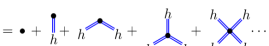
Figure 1: Schematic representation of the vertex expansion of the effective action $\Gamma[\bar{g},h]$. Blue double lines represent the fluctuating graviton and black dots mark full vertices.

The content of 10 is best illustrated at the example of the transverse-traceless component of the graviton two-point function in a flat background with $\Delta\to p^{2}$ with the parametrisation

$$\Gamma_{\textrm{tt}}^{(2,0)}(p)= \,\frac{1}{16\pi G_{N}}\,Z_{g}(p)\,p^{2}\,\Pi_{\textrm{tt}}\,,$$

$$\Gamma_{\textrm{tt}}^{(0,2)}(p)= \,\frac{1}{16\pi}Z_{h}(p)\,p^{2}\,\Pi_{\textrm{tt}}\,.$$ (12)

The tt-projection operator $\Pi_{\textrm{tt}}$ is provided in 47 in Appendix C. We have normalised the wave function of the background graviton with ${Z_{g}(p=0)=1}$, which fixes the Newton constant as the infrared or classical one. Inserting 12 into 10 leads us to

$$G(p)=\frac{G_{N}}{Z_{g}(p)}\,,$$ (13)

which fixes the prefactor $G(p)$ in 2 as the inverse wave function of the transverse-traceless background graviton, $Z_{g}$, multiplied by the classical Newton constant $G_{N}$.

Equation 13 encodes the well-known relation that the inverse wave function of the background field in the background field approach carries the running coupling of the theory. Indeed, 13 should rather be seen as the definition of a running Newton coupling for the reasons explained around 8.

Note that in terms of the diffeomorphism-covariant correlation functions $\Gamma^{(n)}$, the wave function $Z_{g}(p)$ receives contributions from different diffeomorphism-invariant terms in the effective action. In the approximation used here, it is a weighted sum of contributions or (two-point) couplings of the $\cal R$- and $R_{\mu\nu}^{2}$-terms in 7. Accordingly, while the inversion of $Z_{g}(p)$ makes sense for defining an average two-point function coupling, for higher correlation functions we first have to disentangle the different invariants in the sum before doing an inversion of the parts.

While this can be done with a sum over general tensor structures, we now restrict ourselves to that used in the present work: On the left hand side of 10 we use results for the completely tt part of the vertices at the momentum symmetric point, and parametrise the $n$-point functions as

$$\Gamma_{\textrm{tt}}^{(n)}(\bm{p}) =\gamma^{(n)}_{g}(p)\,\mathcal{T}_{R,\textrm{tt}}^{(n)}(\bm{p})\,.$$ (14)

where $\bm{p}=(p_{1},...,p_{n})$, $p=|p_{i}|$ and $\mathcal{T}_{R,\textrm{tt}}^{(n)}$ is the completely transverse-traceless projection of the $n^{\text{th}}$-derivatives of the curvature part of the Einstein-Hilbert action, see 48 in Appendix C. There it is also detailed how to project $\Gamma^{(n)}$ on the tt-coefficient $\gamma_{g}^{(n)}$, see 51. Note, that due to our choice of the tensor structures the vertex coefficients $\gamma_{g}^{(n)}$ have momentum dimension two, ${[\gamma_{g}^{(n)}]=2}$, in analogy with the classical theory where $[G_{N}^{\phantom{N}-1}]=2$.

In the present work we compute the fluctuation vertices $\Gamma^{(0,n)}$ and use the approximated Nielsen identity 10 to extract the coefficients $\gamma_{g}^{(n)}$ of the $n$-point functions of the diffeomorphism-invariant action 6 from these results. Accordingly, we can already parametrise the $\Gamma^{(0,n)}$ in terms of $\gamma_{g}^{(n)}$, to wit,

$$\Gamma_{\textrm{tt}}^{(0,n)}(\bm{p}) =\,\prod_{i=1}^{n}\sqrt{Z_{h}(p_{i})\,G(p_{i})}\,\gamma_{g}^{(n)}(p)\,\mathcal{T}_{R,\textrm{tt}}^{(n)}(\bm{p})\,.$$ (15)

The projection of the full $\Gamma^{(0,n)}$ onto $\Gamma_{\textrm{tt}}^{(0,n)}$ is detailed in Appendix C, see 50.

We note in this context, that the vertex couplings, which genuinely drive the dynamics in the fluctuation approach, are not the $\gamma_{g}^{(n)}$, but rather the coupling coefficients $\gamma_{h}^{(n)}(\bm{p})$ given by

$$\gamma_{h}^{(n)}(\bm{p})=\prod_{i=1}^{n}\sqrt{G(p_{i})}\gamma_{g}^{(n)}(\bm{p})\,.$$ (16)

These are the coefficients of the RG-invariant core $\bar{\Gamma}^{(0,n)}$ of the fluctuation $n$-point functions,

$$\bar{\Gamma}^{(0,n)}(\bm{p})=\frac{\Gamma^{(0,n)}(\bm{p})}{\prod_{i=1}^{n}\sqrt{Z_{h}(p_{i})}}\,.$$ (17)

Equation 17 naturally occurs in diagrams as all fluctuation propagators carry a $1/Z_{h}$, and a factor $1/Z_{h}^{1/2}$ can be assigned to each vertex these propagators are connected to. In short, the loop diagrams in functional approaches, which are built from full vertices and propagators, reduce to diagrams with classical propagators and $\bar{\Gamma}^{(0,n)}$ vertices. Hence, these vertices carry the full quantum dynamics of the theory. Finally, 17 is simply the non-perturbative analogue of the standard perturbative definition of the running coupling from vertices and propagators. By now, the relevance as well as significance of 17 in non-perturbative expansion schemes has been evaluated and shown in both, QCD and asymptotically safe gravity, for respective reviews see [29, 6, 30].

In order to clarify the meaning of the yet undetermined coefficient $G(p)$, as defined in 13, we use that both, $\Gamma_{\textrm{tt}}^{(2)}$ and $\Gamma_{\textrm{tt}}^{(3)}$, only receive contributions from $\cal R$ and the Ricci tensor part of the effective action 7. Hence, in a last approximation step we identify $\gamma_{g}^{(2)}$ and $\gamma_{g}^{(3)}$, leading to

$$G(p)=\left[\gamma_{h}^{(3)}(p)\right]^{2}=\left[\gamma_{g}^{(3)}(p)\right]^{-1}\,,$$ (18)

where we have used $\gamma_{h}^{(2)}=1$. Note also, that the relation 18 and similar ones for higher $n$-point functions suggest the definition ${\gamma_{h}^{(n)}=G_{n}^{n/2-1}}$. Here, the $G_{n}$ are referred to as avatars of the Newton coupling, see [10, 31, 32, 6]. However, for the present purpose of reconstructing the effective action in terms of curvature invariants this parametrisation is not suggestive and we will not use it here.

In summary, we are led to a systematic expansion of the full diffeomorphism-invariant action $\Gamma[g]$. Note that this is a non-perturbative expansion, as all the vertices appearing in Figure 1 are fully dressed. The present expansion 7 in powers of the curvature suggests to expand the effective action in terms of correlation functions on a flat Euclidean background

$$\bar{g}_{\mu\nu}=\delta_{\mu\nu}\,,$$ (19)

where all curvature invariants vanish, i.e. $R=0$ and ${R_{\mu\nu}^{2}=0}$. This simplifies computations considerably, as they can be done in momentum space. Expansions about different backgrounds have been considered e.g. in [33, 34]. Promising signs of apparent convergence of the vertex expansion about a flat background have been observed in [10] upon gradually improving the truncation, by computing the full running vertices up to the four-point function.

The analysis in the present work is based on a fRG computation of momentum-dependent fluctuation two-, three- and four-graviton correlation functions, $\Gamma^{(0,n)}$ with $n=2,3,4$, building on the computation in [10]. While in the latter work the full momentum dependence was already provided implicitly in terms of the ultraviolet-infrared flows, we will integrate these results in the present work. The fRG computation is described in the following Section III, further details can be found in [10, 6].

III Functional renormalisation group flows for gravity

For the computation of the momentum-dependent two-, three- and four-point function we employ the functional renormalisation group, for recent reviews including quantum gravity see [29, 35]. In this approach, quantum fluctuations are integrated out successively by introducing a momentum-dependent mass term with the mass function $\mathcal{R}_{k}$ to the classical dispersion. Such a deformation suppresses fluctuations with momenta $p^{2}\lesssim k^{2}$ below the IR cutoff scale $k$, and leaves the UV-regime with $p^{2}\gtrsim k^{2}$ unchanged. The flow of the scale-dependent effective action is given by the Wetterich equation [36] for quantum gravity [2],

$$\partial_{t}\Gamma_{k}[\bar{g},h]=\frac{1}{2}\text{Tr}\,\mathcal{G}_{k}[\bar{g},h]\,\partial_{t}\mathcal{R}_{k}\,.$$ (20a)

In 20a we used the definitions $${\partial_{t}=k\partial_{k}} \mathcal{G} \phi=(h_{\mu\nu},c_{\mu},\bar{c}_{\mu})$$ and is the full, field-dependent propagator of the fluctuation fields defined in 42,

$$\mathcal{G}_{k}[\bar{g},h]=\frac{1}{\Gamma_{k}^{(0,2)}[\bar{g},h]+\mathcal{R}_{k}}\,,$$ (20b)

where we drop the ghost field argument, as all our correlation functions are evaluated at vanishing ghost fields, $(c_{\mu},\bar{c}_{\mu})=0$. The trace operator Tr incorporates a sum over all fluctuation fields $\phi$, Lorentz indices and an integral over momenta or spacetime, and includes a minus sign for the Grassmann-valued ghost fields. A graphical depiction is provided in Figure 2.

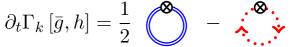
Figure 2: Diagrammatic representation of the Wetterich equation. The blue double line represents the fluctuating graviton, the dotted line denotes the ghost field. The crossed circle indicates the insertion of a regulator derivative, $\otimes=\partial_{t}\mathcal{R}_{k}$.

III.1 Flows for $n$-point functions

The flows of the 1PI $n$-point correlation functions are derived from the functional flow equation 20 by taking $n$-field derivatives w.r.t. to the fields $\bar{g}\,,\phi$. Inserting the parametrisation 15 of $\Gamma_{\textrm{tt}}^{(0,n)}$ into the flow equation allows one to extract momentum-dependent, non-perturbative beta functions for the couplings $\gamma_{h}^{(n)}$ defined in 16. These flows give rise to UV fixed points and asymptotically safe RG trajectories. Here we build upon the results in [7, 8, 9], and in particular [10, 11] where the momentum dependence of fluctuation and background correlation functions has been resolved up to the graviton four-point function. Results for the momentum-dependent propagators and running Newton coupling have been provided directly in [11], but the momentum dependence of the vertices has only be given implicitly in terms of the flows. Using this existing data, in the present work we integrated the fully momentum-dependent flow of the four-point function, which is depicted diagrammatically in Figure 3. This provides, for the first time, the full momentum dependence of the graviton four-point function $\Gamma^{(4)}(p)$ at the physical cutoff scale $k=0$.

We defer the discussion of our approximations and technical details of the full computation to Appendix E and proceed with the discussion of our results, which are summarised in Figure 4.

Figure 3: Diagrammatic representation of the flow of the graviton four-point function. All vertices and propagators are fully dressed. Reproduced from [10].

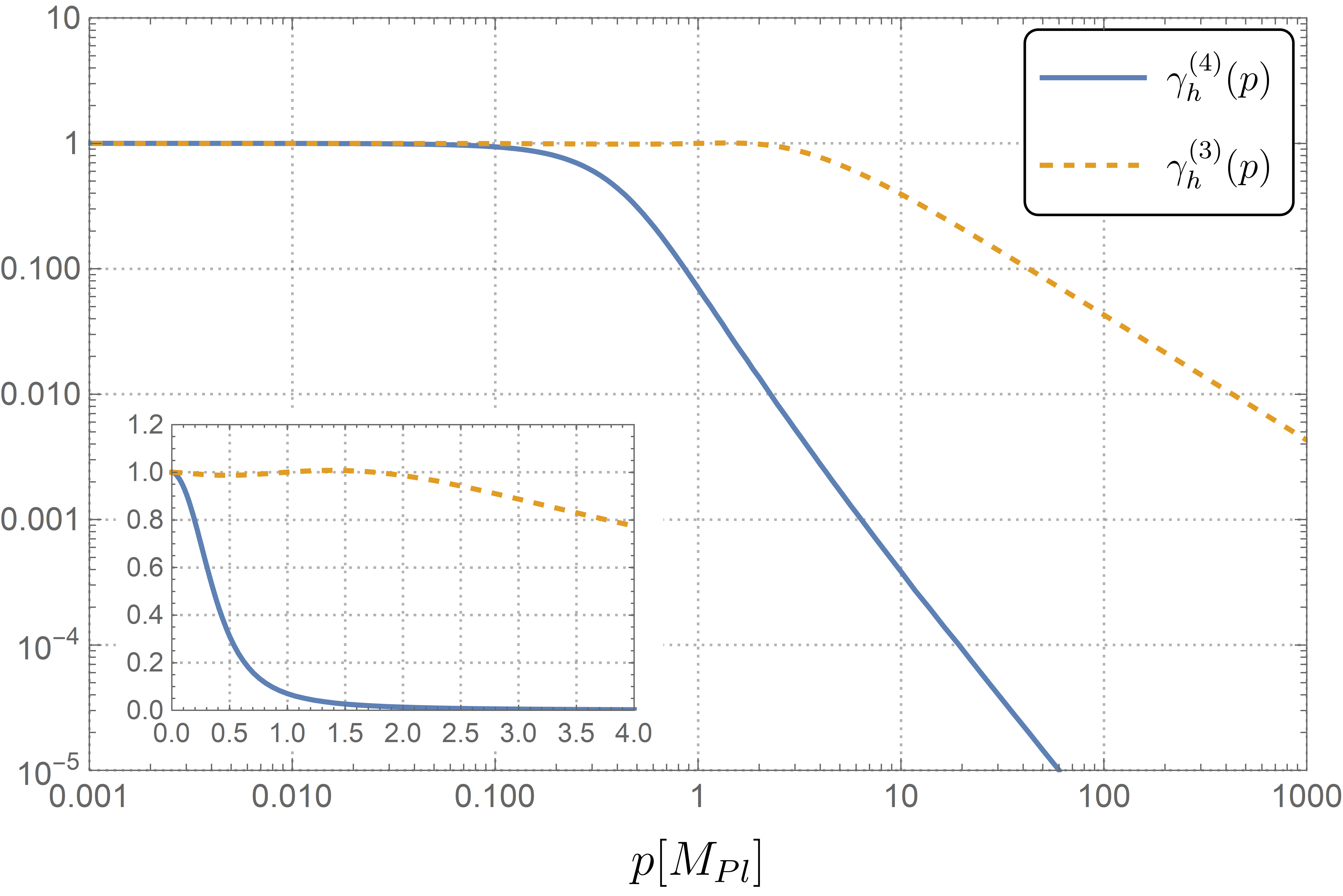
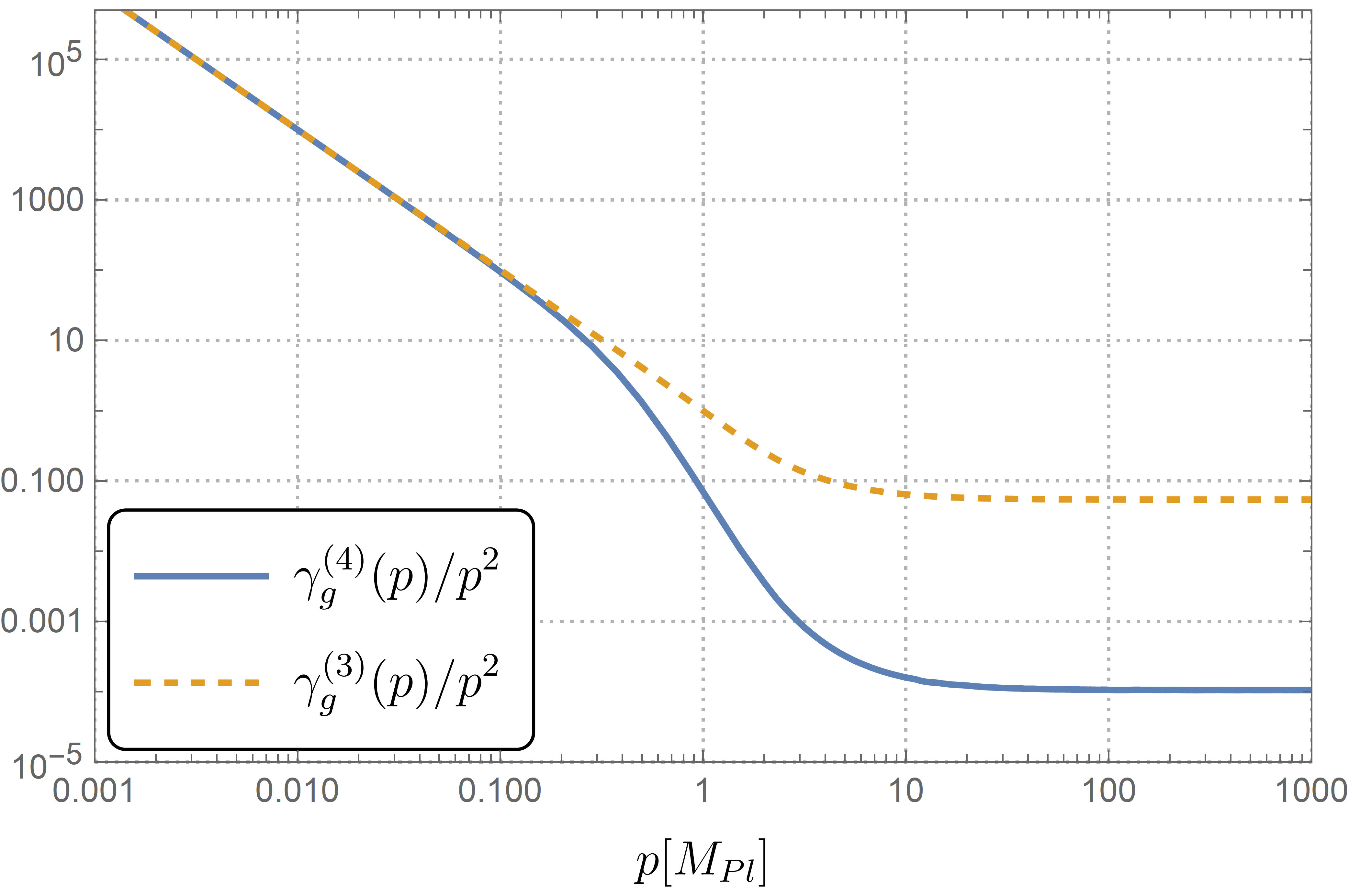
Figure 4: Momentum dependence of the fluctuation (left) and background (right) couplings of the three- and four-graviton vertex in the physical limit $k\rightarrow 0$. The dimensionful fluctuation couplings $\gamma_{h}^{(4)}(p)$ (blue) and $\gamma_{h}^{(3)}(p)$ (dashed) approach a constant value in the IR, given by the Newton coupling $(\gamma_{h}^{(3)})^{2}(0)=\gamma_{h}^{(4)}(0)=G_{N}\equiv 1$. $\gamma_{h}^{(4)}(p)$ turns to the asymptotically safe running $\propto p^{-2}$ roughly one order of magnitude earlier than $\gamma_{h}^{(3)}(p)$, which runs as $\propto p^{-1}$ due to its mass dimension $[\gamma_{h}^{(3)}]=-1$. The inset shows the same data plotted linearly. The dimensionless background couplings $\gamma_{g}^{(4)}(p)/p^{2}$ (blue) and $\gamma_{g}^{(3)}/p^{2}$ (dashed) scale $\propto p^{-2}$ in the IR and go to a constant in the UV fixed point regime. The data used for $\gamma_{g,h}^{(3)}(p)$ was computed in [11].

There, we display the momentum-dependent fluctuation coupling $\gamma_{h}^{(4)}(p)$ of the four-graviton vertex at vanishing cutoff $k=0$. It constitutes a key result of this work. We find a classical regime $p\ll M_{\text{Pl}}$, where the coupling is constant and $\gamma_{h}^{(4)}(0)=G_{N}$. Towards the fixed point regime above the Planck scale we see asymptotically safe scaling $\propto p^{-2}$, reflecting the mass dimension ${[\gamma_{h}^{(4)}]=-2}$. Interestingly, the coupling $\gamma_{h}^{(4)}(p)$ shows the non-trivial scaling behaviour already roughly one order of magnitude below the Planck scale and before its lower counterpart $\gamma_{h}^{(3)}(p)$, which is constructed from data computed in [11]. This is due to the fact that the fixed point values of the dimensionless couplings 46 satisfy $g_{3}^{*}>g_{4}^{*}$. Our finding implies that the quantum regime of asymptotically safe gravity already leads to non-trivial signatures one order of magnitude below the Planck scale. Analytic fits to the numerical data are provided in Appendix H.

On the right-hand side of Figure 4 we display the dimensionless counterparts $\gamma_{g}^{(4)}(p)/p^{2}$ and $\gamma_{g}^{(3)}(p)/p^{2}$ of the background couplings, which are computed from the fluctuation couplings by means of the relation 16. They show canonical scaling $\propto p^{-2}$ in the classical regime and take constant values in the UV, as required by asymptotic safety.

IV Form factors

We now discuss the reconstruction of the form factor factors $f_{R^{2}}(p^{2})$ and $f_{R_{\mu\nu}^{2}}(p^{2})$ introduced in 7 from the momentum-dependent background couplings $\gamma_{g}^{(3)}(p)$ and $\gamma_{g}^{(4)}(p)$ at hand.

In a first step we project the $n$-point functions on the curvature part of the Einstein-Hilbert action by contracting them with $\mathcal{T}_{R,\textrm{tt}}^{(n)}$. This projection of the background $n$-point functions 14 results in the scalar expression

$$\Gamma_{\textrm{tt}}^{(n)}\circ\mathcal{T}_{R,\textrm{tt}}^{(n)}/p^{2}=C_{R}^{(n)}\gamma_{g}^{(n)}p^{2}\,,$$ (21)

where the division with $p^{2}$ eliminates the dispersion part of the tensor structure and $\circ$ denotes the pairwise contraction of Lorentz indices. The projection scheme is described in more detail in Appendix C and the values of the coefficients $C_{R}^{(n)}$ are given in 54.

The projection leading to 21 is now also applied to the $n$-point functions resulting from respective field derivatives of 7. Equating the two sides results in

$$C_{R}^{(n)}\gamma_{g}^{(n)}p^{2}=C_{\mathcal{R}}^{(n)}g_{\mathcal{R}}p^{2}+C_{R^{2}}^{(n)}f_{R^{2}}p^{4}+C_{R_{\mu\nu}^{2}}^{(n)}f_{R_{\mu\nu}^{2}}p^{4}\,,$$ (22)

where the coefficients $C_{\mathcal{O}}^{(n)}$ are given explicitly in 54. These preparations enable us to read-off the form factors. We start with the Ricci tensor form factor, which is obtained for $n=3$,

$$f_{R_{\mu\nu}^{2}}(p^{2})=\frac{1}{C_{R_{\mu\nu}^{2}}^{(3)}}\frac{C_{R}^{(3)}\gamma_{g}^{(3)}-C_{\mathcal{R}}^{(3)}g_{\mathcal{R}}}{p^{2}}\,,$$ (23)

where we used that $C_{R^{2}}^{(3)}=0$ due to the tt-projection. The $R^{2}$ form factor is computed from the four-point function, $n=4$. Equation 22 results in

$$f_{R^{2}}(p^{2})=\frac{1}{C_{R^{2}}^{(4)}}\frac{C_{R}^{(4)}\gamma_{g}^{(4)}-C_{\mathcal{R}}^{(4)}g_{\mathcal{R}}-C_{R_{\mu\nu}^{2}}^{(4)}f_{R_{\mu\nu}^{2}}p^{2}}{p^{2}}\,.$$ (24)

It is left to reconstruct the ${\mathcal{R}}(\Delta,R)$-term, that encodes the classical curvature term in the IR. In order to satisfy the required limits 9 we choose

$$\mathcal{R}(\Delta,R)=R\frac{\gamma_{g}^{(3)}(\Delta)-\bar{\gamma}_{3}\Delta}{\Delta+R}R\,,$$ (25)

with the dimensionless constant $\bar{\gamma}_{3}$ defined in 63 in Appendix F. Equation 25 generates a $p^{2}$ contribution to the flow of the $n$-point functions ${\Gamma}_{G}^{(n)}(p)$ with the prefactor given by ${g_{\mathcal{R}}=\gamma_{g}^{(3)}(0)=G_{N}^{-1}}$, in accordance with the classical limit. This is shown in Appendix F. The denominator is a sum of the curvature scalar $R$ and the Laplace-Beltrami operator $\Delta$. The latter part arranges for the necessary disappearance of the curvature term in the UV with large spectral values of $\Delta$. In turn, in the IR with small spectral values of $\Delta$, 25 reduces to $\gamma_{g}^{(3)}(0)\,R$. We emphasise that the structure of 25 is fixed, but the general denominator in 25 is given by a weighted sum of $R$ and $\Delta$.

In Figure 5 the form factors $f_{R_{\mu\nu}^{2}}(p^{2})$ and $f_{R^{2}}(p^{2})$ are plotted as a function of the physical momentum $p$. Both form factors approach constant values in the IR as well as in the UV. The values resulting from our numerical data are given in Appendix G, 66 and 67 respectively. We observe that the UV values are one to two orders of magnitude smaller than their IR counterparts. Furthermore, we note that $f_{R_{\mu\nu}^{2}}(p^{2})$ is negative both in the IR and UV and its absolute value is smaller than $f_{R^{2}}(p^{2})$ everywhere.

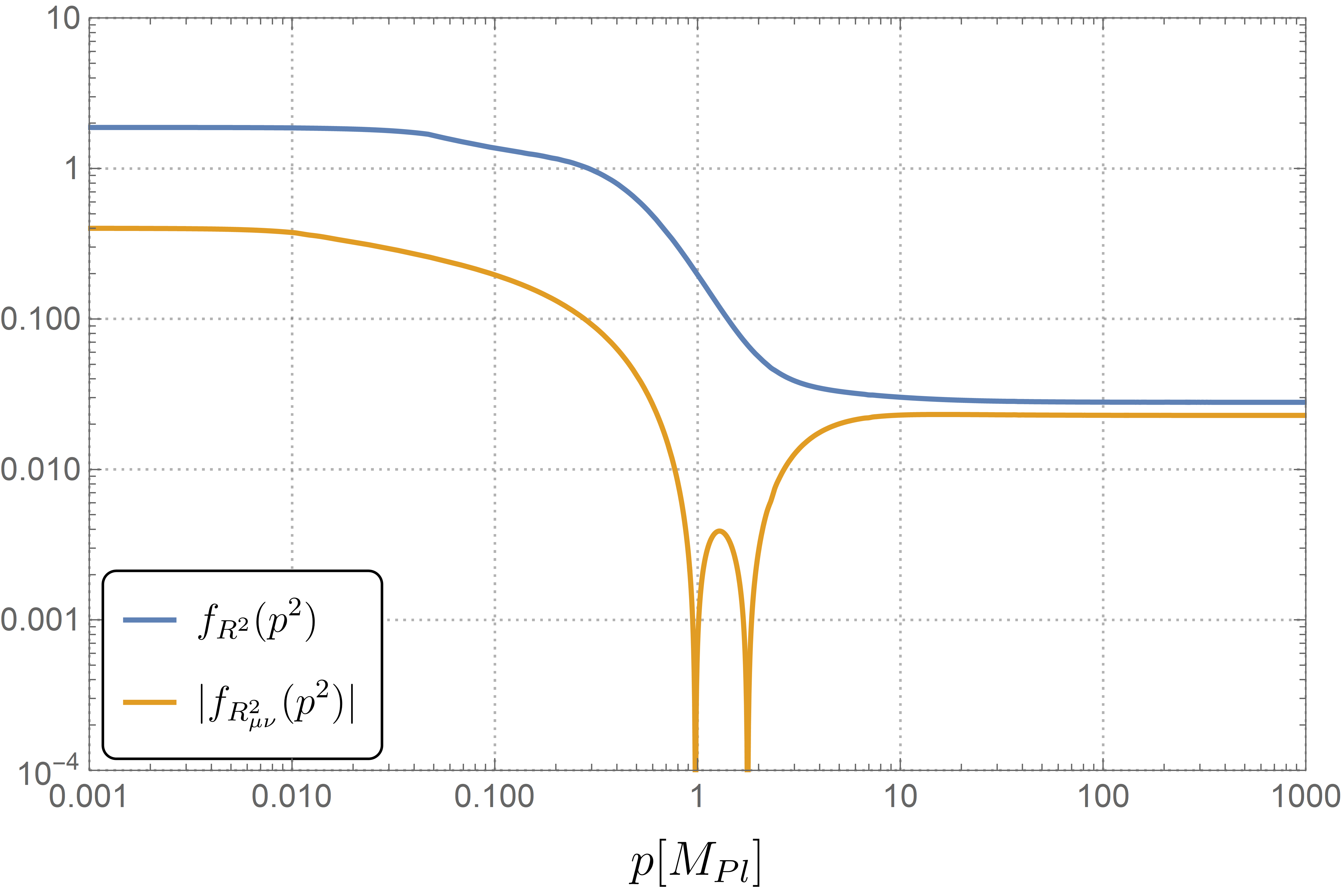
Figure 5: The form factors $f_{R_{\mu\nu}^{2}}(p^{2})$ 23 and $f_{R^{2}}(p^{2})$ 24 as a function of physical momentum $p$. Both attain constant values in the IR as well as in the UV. Note that $f_{R_{\mu\nu}^{2}}$ is negative over almost the entire momentum range, except near $p\approx 1$, and $|f_{R_{\mu\nu}^{2}}|<f_{R^{2}}$ everywhere.

For practical applications we derive very simple analytic expressions, that interpolate between the IR and UV asymptotes of $f_{R_{\mu\nu}^{2}}$ and $f_{R^{2}}$. Substituting ${p^{2}\to\Delta}$, in position space these are given by

$$f_{R_{\mu\nu}^{2}}(\Delta) \simeq\tilde{g}_{R_{\mu\nu}^{2}}+\frac{g_{R_{\mu\nu}^{2}}-\tilde{g}_{R_{\mu\nu}^{2}}}{1+p_{0}^{-2}\Delta}\,,$$

$$f_{R^{2}}(\Delta) \simeq\tilde{g}_{R^{2}}+\frac{g_{R^{2}}-\tilde{g}_{R^{2}}}{1+p_{1}^{-2}\Delta}\,,$$ (26)

with $p_{0}$ and $p_{1}$ expressed in units of the Planck mass $p_{i}/M_{\text{Pl}}$ and the numerical values of the constants given in 66, 67 and 74 respectively. These expressions capture the correct limits of the form factors as ${\Delta\to 0}$ and ${\Delta\to\infty}$. More elaborate fits to the numerical data are provided in Appendix H, see 75 and 77. Importantly, we find that the form factors introduce non-local contributions in the effective action due to the appearance of the inverse Laplace operator $\Delta^{-1}$.

Finally, we study the infrared behaviour of the form factor expressions 23, 24, 25 and 26. By construction, the operator $\mathcal{R}(\Delta,R)$ in 25 reduces to the Einstein-Hilbert term, see 9. The low energy limit of the form factors is found by Taylor expanding the analytic expressions 75 and 77 about $p^{2}=0$ to first order. In position space this yields

$$f_{R_{\mu\nu}^{2}}(\Delta) \simeq g_{R_{\mu\nu}^{2}}+c_{1}\Delta\,,$$

$$f_{R^{2}}(\Delta) \simeq g_{{R}^{2}}+c_{2}\Delta\,,$$ (27)

with the values of the coefficients $c_{1,2}$ given in 68. In terms of the vertex dressings $\gamma_{g}^{(3)}$ and $\gamma_{g}^{(4)}$, the constant IR couplings of the $R_{\mu\nu}^{2}$ and $R^{2}$ terms read

$$g_{R_{\mu\nu}^{2}} =c_{3}\left[\gamma_{g}^{(3)}\right]^{\prime}(0)\,,$$

$$g_{R^{2}} =c_{4}\left[\gamma_{g}^{(4)}\right]^{\prime}(0)-c_{5}\left[\gamma_{g}^{(3)}\right]^{\prime}(0)\,,$$ (28)

with the prime denoting a derivative with respect to $p^{2}$ and the constants $c_{3,4,5}$ defined in 69.

The reconstruction of the effective action or rather the form factors is an important result of the present work. It puts forward a systematic way to map the momentum dependent graviton correlation functions to diffeomorphism invariant expressions in the effective action. The approximations used for the explicit computation can be lifted within improved computations. The resulting effective action can be used to address important physics questions, as for example in the context of black hole spacetimes.

V Quantum black hole solutions

Asymptotic safety dictates a specific form of scale-dependence of the gravitational coupling in the UV, which is expected to ultimately resolve the curvature singularities in the classical theory. The implications of ”quantum-improving” classical black hole spacetimes by promoting the classical Newton constant $G_{N}$ to a scale-dependent quantity have received a lot of attention [37, 38, 39, 40, 41, 42, 43, 44, 45, 46, 47, 48, 49, 50, 51], see [52] for a recent review. This procedure is expected to capture the leading order quantum effects and interesting implications have been reported. However, the identification of the IR cutoff $k$ with a physical scale is not unique in gravity and different choices can result in physically distinct spacetimes. Moreover, this RG improvement can introduce unphysical coordinate dependencies [53] and physical conclusions have to be drawn with care. For a fully consistent picture of quantum black hole spacetimes a different approach is needed.

To capture the causal structure of a given spacetime geometry, it is essential to consider the theory in Lorentzian signature. Therefore, at this point we perform a Wick rotation on our Euclidean results and denote this by replacing the Euclidean Laplace operator by the full d’Alembertian, $\Delta\to\Box$.

Based on studies of the relation between Euclidean and Lorentzian asymptotically safe gravity [54], we expect that the main features of our results carry over to the theory in physical signature, although the Wick rotation in curved spacetime is still not fully understood [55, 56, 57].

V.1 Effective field equations

In order to address the question how black holes are modified in the quantum theory, we solve the field equations resulting from the effective action $\Gamma[\bar{g}]$ 7. In a slight abuse of notation we will write $g_{\mu\nu}$ when we actually refer to the background metric $\bar{g}_{\mu\nu}$ in this section.

If we neglect the $g_{\mu\nu}$ dependence of the form factors themselves, we can straightforwardly derive the field equations resulting from the second two terms in 7. Dropping boundary terms that arise from partial integration, the term ${Rf_{R^{2}}(\Box)R}$ results in the field equations

$$2\left(R_{\mu\nu}-\frac{1}{4}Rg_{\mu\nu}+g_{\mu\nu}\Box-\nabla_{\mu}\nabla_{\nu}\right)f_{R^{2}}(\Box)R=0\,,$$ (29)

and variation of the term ${R_{\mu\nu}f_{R_{\mu\nu}^{2}}(\Box)R^{\mu\nu}}$ results in

$$\left(2R_{\mu\sigma}g_{\nu\rho}-\frac{1}{2}g_{\mu\nu}R_{\rho\sigma}+g_{\rho\mu}g_{\sigma\nu}\Box\right)f_{R_{\mu\nu}^{2}}(\Box)R^{\rho\sigma}$$

$$\hskip 17.07182pt+\left(g_{\mu\nu}\nabla_{\rho}\nabla_{\sigma}-2g_{\mu\sigma}\nabla_{\rho}\nabla_{\nu}\right)f_{R_{\mu\nu}^{2}}(\Box)R^{\rho\sigma}=0\,.$$ (30)

One recognizes the similarity to the field equations of quadratic gravity [58], but with the constant couplings replaced by non-trivial form factors acting on the Ricci scalar $R$ and tensor $R^{\rho\sigma}$.

In order to generalise the classical Einstein-Hilbert term in a diffeomorphism invariant fashion we constructed the operator $\mathcal{R}(\Box,R)$ containing the non-local term $(\square+R)^{-1}$. The form factors $f_{R_{\mu\nu}^{2}}(\Box)$ and $f_{R^{2}}(\Box)$ also contain such non-local operators, c.f. the analytic fits 26, 75 and 77. This poses a non-trivial issue for numerical computations, because inverse differential operators are generically difficult to deal with and require finding Green’s functions $\mathcal{G}(x,x^{\prime})$ which solve

$$(\Box+R)\mathcal{G}(x,x^{\prime})=\frac{1}{\sqrt{-g}}\ \delta(x-x^{\prime})\,,$$ (31)

on general curved backgrounds [55, 59]. This task could be tackled e.g. by expanding $\mathcal{G}(x,x^{\prime})$ about the Feynman propagator in flat space, $\mathcal{D}_{\text{F}}(x,x^{\prime})$, or by means of an eigenfunction expansion using numerical techniques. Alternatively, one could implement an iterative procedure by starting with some initial guess for the Green’s function, using it to compute solutions to the field equations and inserting these back into 31 in order to improve the initial guess. This is beyond the scope of the present paper, however, and we leave a more thorough analysis to future work. For recent studies involving non-local terms in the context of black holes see [22, 23].

Here, we will instead focus on investigating the dominant IR quantum gravity effects. Inserting the IR limits of the form factor expressions in 27, Equation 7 results in the infrared effective action $\Gamma_{\text{IR}}[g]$

$$\Gamma_{\text{IR}}[g_{\mu\nu}]=\frac{1}{16\pi}\int_{x}\sqrt{-g}\big{(}G_{N}^{-1}R+g_{R_{\mu\nu}^{2}}R_{\mu\nu}R^{\mu\nu}$$

$$+g_{R^{2}}R^{2}+c_{1}R_{\mu\nu}\Box R^{\mu\nu}+c_{2}R\Box R\big{)}\,.$$ (32)

The field equations resulting from 32 are obtained by simply inserting 27 into 29 and 30, together with Einstein’s field equations resulting from the Einstein-Hilbert part.

We expect the effective action 32 to capture the most relevant corrections to the classical theory, that might be detectable in future gravitational wave observatories or Event Horizon Telescope images.

V.2 Spherically symmetric solutions

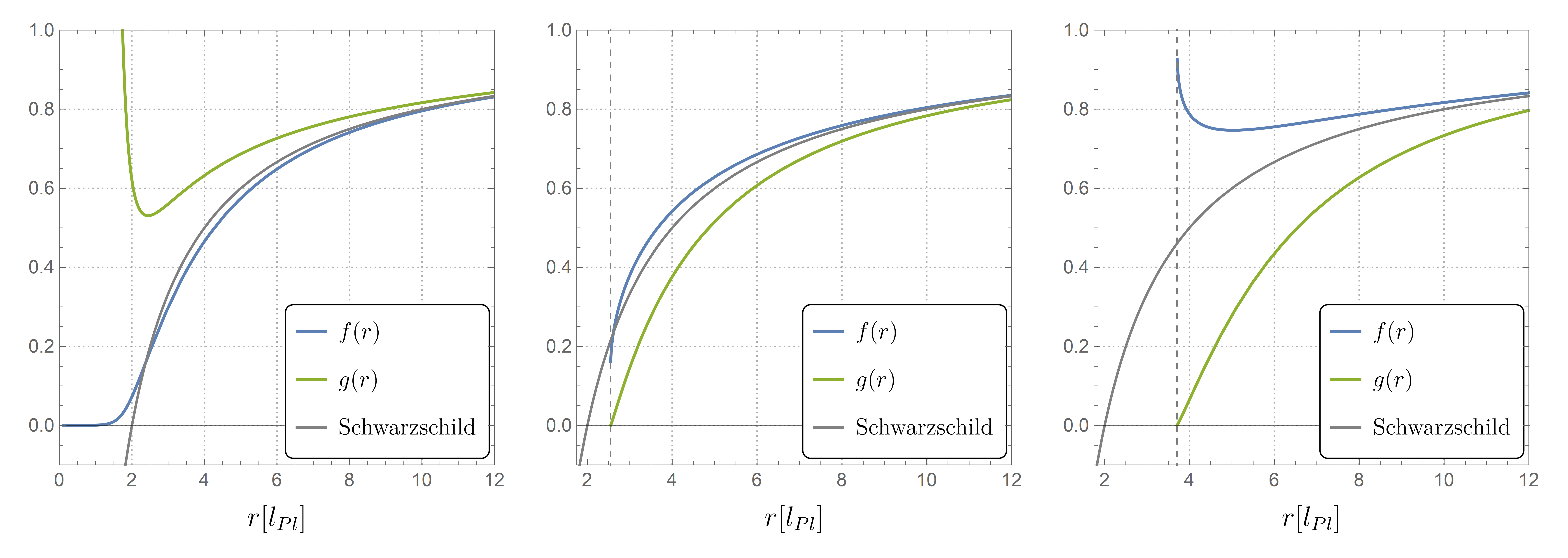
Figure 6: Examples of spherically symmetric solutions for $S_{2}=1$ and $M=1$. The solutions containing a zero-crossing $r_{h}$ are plotted only up to that radius, marked by a dashed line. The type I solution on the left has $S_{0}=-1$, the type II solution in the middle is found for $S_{0}=1$ and the type III solution shown on the right has $S_{0}=4$.

We restrict ourselves to static, spherically symmetric metrics. The most general ansatz for such metrics in Schwarzschild coordinates reads

$$ds^{2}=-f(r)\text{d}t^{2}+\frac{1}{g(r)}\text{d}r^{2}+r^{2}d\Omega^{2}\,,$$ (33)

with two a priori independent lapse functions $f(r)$ and $g(r)$ depending on the radial coordinate $r$ only. The angular element $d\Omega^{2}$ is defined by

$$d\Omega^{2}=\text{d}\theta^{2}+\text{sin}^{2}(\theta)\text{d}\varphi^{2}\,.$$ (34)

The classical Schwarzschild metric is obtained for ${f(r)=g(r)=1-2M/r}$, where $M$ corresponds to the mass of the black hole that would be measured by an observer at infinity. As initial conditions for the numerical integration we make use of the well-known weak-field limit of classical quadratic gravity, first studied in [58]. It is found by perturbing the metric and linearising the field equations resulting from the terms $R+R^{2}+R_{\mu\nu}^{2}$, which give the dominant contributions at small curvatures. Then, imposing asymptotic flatness results in the weak field solutions

$$f(r) =1-\frac{2M}{r}+S_{0}\frac{e^{-m_{0}r}}{r}+S_{2}\frac{e^{-m_{2}r}}{r}\,,$$

$$g(r) =1-\frac{2M}{r}-S_{0}\frac{e^{-m_{0}r}}{r}(1+m_{0}r)$$

$$\phantom{=1-\frac{2M}{r})}+\frac{1}{2}S_{2}\frac{e^{-m_{2}r}}{r}(1+m_{2}r)\,,$$ (35)

where the two free parameters $S_{0}$ and $S_{2}$ determine the strength of the exponentially decaying Yukawa corrections. The masses $m_{0}$ and $m_{2}$ of the spin-0 and spin-2 modes, respectively, are related to the couplings of the different curvature terms and are given in 70.

We choose to initialise our integration at the radius $r_{in}=20$, which is located in a regime far enough from the horizon such that the curvature is still small, but the exponential corrections in 35 are still sizeable enough to be captured by the numerics. Inserting this ansatz for the metric into the field equations leads to equations of motion containing up to 6 derivatives in the radial coordinate $r$. The resulting system of coupled differential equations is then integrated numerically towards $r\rightarrow 0$ for different initial values $(M,S_{0},S_{2})$.

For the initial conditions $(S_{0},S_{2})=(0,0)$ with $M=1$ we recover the classical Schwarzschild metric, as expected. The event horizon at $r_{S}=2$ is defined by the zero-crossing $f(r_{S})=g(r_{S})=0$. When the geometry contains a radius $r_{h}$ where $f(r_{h})=0$ or $g(r_{h})=0$, one cannot continue the integration towards $r=0$. In studies of spherically symmetric solutions of quadratic gravity [60, 61, 62, 63, 64, 65, 66, 67, 68, 69] this issue is dealt with by using an analytic expansion of the metric near the horizon in combination with a shooting method for the numerical integration. However, as we are considering an IR expansion of the form factors, the solutions will not be reliable in the high curvature regime below the horizon and thus we refrain from improving the numerical strategy in this regime.

Subsequently, we consider $M=1$ and non-zero initial values for $(S_{0},S_{2})$. Firstly, we observe that the behaviour of a solution is essentially determined by the value of $S_{0}$. This is because for our values of the couplings $m_{2}>m_{0}$, see 70, and therefore the terms $\propto S_{2}$ in the initial conditions 35 are suppressed. Therefore we focus our discussion on the dependence of the solutions on $S_{0}$ at fixed $S_{2}$. Depending on the value of $S_{0}$, the solutions can be classified into three types. One example of each type is shown in Figure 6.

Negative values of $S_{0}$ result in type I solutions. These are horizon-less geometries where the metric remains regular at the origin. Here, $f(r)$ vanishes towards the origin, whereas $g(r)$ diverges. However, the Kretschmann scalar of these solutions diverges at the origin, hinting at a naked singularity.

For positive values of $S_{0}$ the solutions contain a radius $r_{h}$ where $g(r_{h})=0$. This $r_{h}$ coincides with the classical Schwarzschild horizon $r_{S}$ for $S_{0}=0$. The larger $S_{0}$, the further $r_{h}$ is shifted to larger radii. The dependence of $r_{h}$ on $S_{0}$ is found to be approximately linear, ${r_{h}(S_{0})\propto S_{0}}$.

When $S_{0}$ remains smaller than a critical value $S_{0,\text{c}}$ we find modified black-hole solutions, which we label type II. In these geometries, both $f(r)$ and $g(r)$ go to zero at $r_{h}$, indicating the presence of a horizon.

For values of $S_{0}$ larger than $S_{0,\text{c}}$, we also have $g(r_{h})=0$ but $f(r)$ instead diverges to $+\infty$ at $r_{h}$. We refer to these exotic geometries as type III.

Comparing the three classes of solutions, one notices that for type I solutions $g(r)>f(r)$ holds, whereas for types II and III we have $f(r)>g(r)$. Further we note that type II and III solutions can be distinguished by the sign of the derivative $f^{\prime}(r)$ at $r_{h}$, namely $f^{\prime}(r_{h})<0$ for type II and $f^{\prime}(r_{h})>0$ for type III.

In order to map out the phase space of solutions in the $(M,S_{0})$-plane we consider the temperature

$$T=\frac{1}{4\pi}\sqrt{|f^{\prime}(r_{h})g^{\prime}(r_{h})|}\,,$$ (36)

that would be measured by a stationary observer at infinity when the spacetime contains an event horizon [49]. In the case of the Schwarzschild spacetime, 36 reproduces the Hawking temperature ${T_{H}=1/(8\pi M)}$. Although the zero-crossings of our solutions at $r_{h}$ may not mark a physical horizon for all solutions types, 36 can still be used as an order parameter for the classification.

The resulting map $T(M,S_{0})$ is displayed in Figure 7. The color scale indicates the value of the temperature parameter 36 for solutions with different values of $M$ and $S_{0}$. The horizontal dark blue line at $S_{0}=0$ indicates that the temperature of the new solutions with non-zero $S_{0}$ is larger than that of the corresponding Schwarzschild solution. The color gradient from left to right is consistent with the classical expectation, that black holes with small masses are hotter as $T_{H}\propto 1/M$.

However, we also observe a dark blue line where $T(M,S_{0})$ goes to zero, marked by a dashed line in the figure. The dependence of the corresponding $S_{0}$ value on this line is approximately linear in $M$. For solutions on this line $f^{\prime}(r_{h})=0$, causing 36 to vanish. This marks a transition between the type II and III solutions, examples of which are shown in the middle and right panel of Figure 6, respectively. Figure 7 can be understood as a phase diagram of the theory: In the lower right corner of the diagram, below the phase transition line, the geometries are the modified black hole solutions of type II. In the upper left corner, where $S_{0}$ is large, the solutions are of the exotic type III. Type I solutions do not feature a horizon-like radius $r_{h}$, such that the parameter 36 can not be defined in these cases. This type of solutions is located at negative $S_{0}$ values in the phase diagram.

The structure of the phase diagram allows for interesting speculations about the Hawking evaporation and its endpoint. In particular, astrophysical black holes with masses many orders larger than the Planck mass will be located very far on the right of the phase diagram. For $\mathcal{O}(1)$ values of the parameter $S_{0}$ the respective geometries will be of the modified black hole type II and from the outside will resemble the Schwarzschild solution (for non-rotating black holes). Due to Hawking radiation, these black holes would gradually lose mass and move towards the left of the phase diagram (assuming $S_{0}$ stays constant), until they encounter the phase transition line where the temperature according to 36 would vanish and the evaporation would stop. For a discussion of the thermodynamic properties and stability of these possible remnants, a more detailed investigation of the limiting solutions near the phase transition is needed, however.

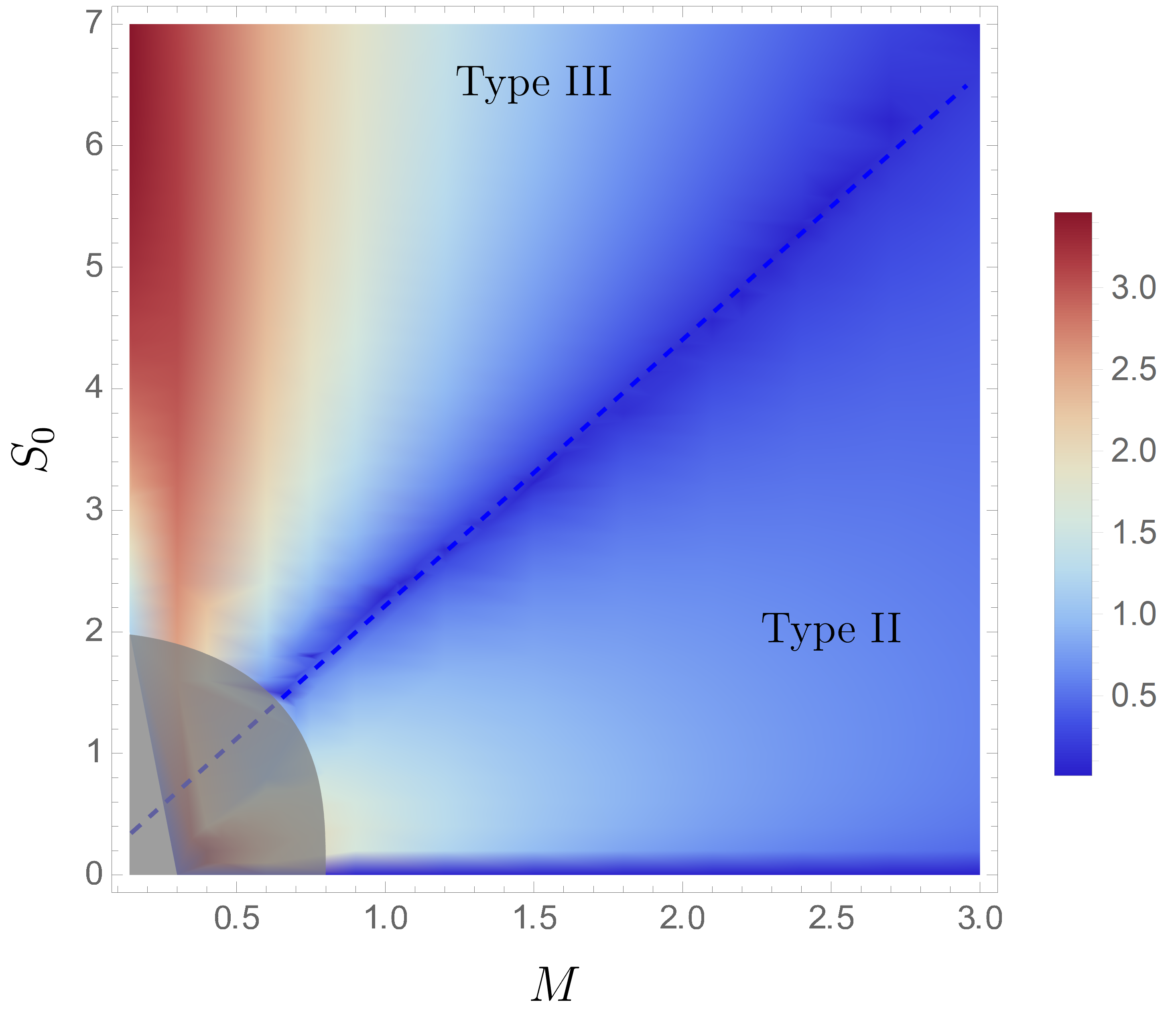
Figure 7: The phase diagram of infrared quantum gravity in the $(M,S_{0})$-plane. The color scale indicates the value of the temperature parameter $T(M,S_{0})$ as defined in 36. The lower right corner is populated by type II solutions, and in the upper left corner type III solutions are found. A dark blue line, where $T(M,S_{0})$ goes to zero, marks the phase transtion between the two solutions types. In the very low $M$ and $S_{0}$ regime in the lower left corner, $r_{h}\rightarrow 0$ and the numerics breaks down close to the origin.

It would be interesting to study the relation between our numerical solutions and other non-Schwarzschild geometries that have been found in higher derivative gravity [60, 61, 62, 63, 64, 65, 66, 67, 68, 69]. In particular it would be interesting to investigate whether the solutions we found can be classified into the same families of solutions in terms of a Frobenius expansion near the horizon. For example, our type I solution in Figure 6 resembles the type II solution plotted in [69], while our type II solution could be related to the non-Schwarzschild black hole or type III solution of [69]. However, for a definitive comparison a more detailed analysis of the causal structure and physical properties of our new geometries is needed and is left for future work.

In [61, 68] it has been argued that in a generic quadratic gravity theory any asymptotically flat solution containing a horizon must have vanishing Ricci scalar $R=0$ in the region outside the horizon. For generic $g_{R^{2}}\neq 0$ and $g_{R_{\mu\nu}^{2}}\neq 0$ this seems to single out the Schwarzschild solution as the only asymptotically flat solution with a horizon (for sufficiently massive black holes). It would be interesting to investigate whether similar restrictive statements apply for our type of action 7 with non-trivial form factors.

In conclusion, we regard it a promising feature that the inclusion of higher order curvature operators in the effective action 32 allows solutions that approach the classical Schwarzschild metric in the IR regime, but show new, non-trivial behaviour at larger curvatures. The above discussion indicates that the higher derivative corrections may alter the classical geometry significantly already outside the classical horizon.

VI Summary

In this work we studied the quantum effective action and black hole solutions in asymptotically safe gravity.

The key object of our investigation is the background effective action $\Gamma[\bar{g}_{\mu\nu}]$, which we studied in detail in Section II. We parametrised $\Gamma[\bar{g}]$ by generalising the classical Einstein-Hilbert term to the operator $\mathcal{R}(\Box,R)$ and by including the two form factors $f_{R_{\mu\nu}^{2}}(\Box)$ and $f_{R^{2}}(\Box)$ to capture higher order effects. These form factors were reconstructed from the momentum-dependent data of graviton $n$-point correlation functions.

In particular, we computed the fluctuation scattering coupling $\gamma_{h}^{(4)}(p)$ of the four-graviton vertex $\Gamma^{(0,4)}$. It shows a classical regime in the IR, where $\gamma_{h}^{(4)}$ is constant, and falls off like $p^{-2}$ in the UV, compatible with AS. It is displayed in Figure 4.

The reconstructed form factors take constant values both in the IR and the UV limits and were found to contain non-local contributions, c.f. 25 and 26. The momentum dependence of $f_{R_{\mu\nu}^{2}}(p^{2})$ and $f_{R^{2}}(p^{2})$ is plotted in Figure 5. Importantly, our work presents a mapping between the scattering-couplings of gravitons and diffeomorphism invariant operators in the effective action.

In Section V we studied spherically symmetric solutions of the effective field equations in our theory. Focussing on low-energy corrections to the classical Schwarzschild black hole, we expanded the form factors about vanishing $p^{2}$, which results in sixth order derivatives in the field equations.

Depending on the initial values for the numerical integration, our solutions can be categorized into three types, displayed in Figure 6. We observed intriguing hints that the quantum corrections may shift the location of the classical horizon and significantly alter the classical geometry already in the near-horizon regime, leading to naked singularities (type I), modified black holes (type II) or exotic type III geometries. It is interesting that the additional degrees of freedom in the field equations allow for solutions that resemble a classical Schwarzschild black hole in the IR but show new, non-trivial features in the UV.

We interpret our results as a promising and important step towards connecting the underlying asymptotically safe theory of quantum gravity to potentially observable consequences for black hole spacetimes.

Appendix A Gauge fixing

We employ a standard linear gauge fixing of the form

$$S_{gf}[\bar{g},h]=\frac{1}{2\alpha}\int_{x}\sqrt{\bar{g}}\ \bar{g}^{\mu\nu}F_{\mu}F_{\nu}\,,$$ (37)

where we choose a de-Donder type gauge-fixing condition

$$F_{\mu}[\bar{g},h]=\bar{\nabla}^{\nu}h_{\mu\nu}-\frac{1+\beta}{4}\bar{\nabla}_{\mu}h^{\nu}_{\phantom{\nu}\nu}\,.$$ (38)

For the gauge parameters $\alpha$ and $\beta$ we choose the harmonic gauge $\beta=1$ and the Landau limit $\alpha\rightarrow 0$. We enforce this condition in the path integral with the Faddeev-Popov method and introduce the ghost fields $c_{\mu}$ and $\bar{c}_{\mu}$. The ghost action reads

$$S_{gh}[\bar{g},h,c,\bar{c}]=\int_{x}\sqrt{\bar{g}}\ \bar{c}^{\mu}\mathcal{M}_{\mu\nu}c^{\nu}\,,$$ (39)

and the Faddeev-Popov operator is defined by

$$\mathcal{M}_{\mu\nu}=\bar{\nabla}^{\rho}\left(g_{\mu\nu}\nabla_{\rho}+g_{\rho\nu}\nabla_{\mu}\right)-\frac{1+\beta}{2}\bar{g}^{\sigma\rho}\bar{\nabla}_{\mu}g_{\nu\sigma}\nabla_{\rho}\,.$$ (40)

Appendix B Vertex expansion

Written explicitly, the vertex expansion of the effective action $\Gamma_{k}[\bar{g},\phi]$ shown in Figure 1 reads

$$\Gamma_{k}[\bar{g},\phi]=\displaystyle\sum_{n=0}^{\infty}\frac{1}{n!}\Gamma_{k}^{(0,\phi_{i_{1}}...\phi_{i_{n}})}[\bar{g},0]\prod_{l=1}^{n}\phi_{i_{l}}\,,$$ (41)

where summation over indices $i_{l}$ that appear twice is understood. In 41 we summarised the fluctuating graviton $h_{\mu\nu}$ and the ghost and anti-ghost fields $c_{\mu}$ and $\bar{c}_{\mu}$ in the fluctuation superfield

$$\phi=(h,\bar{c},c)\,.$$ (42)

In this work we will make a similar ansatz for the $n$-point functions $\Gamma^{(n)}$ as has already been employed in [8, 9, 10, 28, 70]. The considerations explained in Section II.3 amount to the parametrisation of the $n$-point functions

$$\Gamma_{k}^{(0,\phi_{1}...\phi_{n})}(\bm{p})=\left(\prod_{i=1}^{n}Z_{\phi_{i}}^{\frac{1}{2}}(p_{i}^{2})\right)\gamma_{h}^{(n)}(\bm{p})\mathcal{T}^{(\phi_{1}...\phi_{n})}(\bm{p};\Lambda_{n})\,,$$ (43)

where we approximate the complete set of tensor structures $\mathcal{T}^{(\phi_{1}...\phi_{n})}$ by the ones generated by the classical Einstein-Hilbert action 1. The cosmological constant is replaced by $\Lambda\rightarrow\Lambda_{n}$, capturing the momentum-independent part of the correlation functions. The tensor structures $\mathcal{T}^{(\phi_{1}...\phi_{n})}$ are then given by

$$\mathcal{T}_{\textrm{EH}}^{(\phi_{1}...\phi_{n})}(\bm{p};\Lambda_{n})=G_{N}S_{\text{EH}}^{(\phi_{1}...\phi_{n})}(\bm{p};\Lambda\rightarrow\Lambda_{n})\,.$$ (44)

Note that even though we refrain from explicitly including tensor structures derived from higher order curvature invariants, they will typically still be generated by the RG-flow and their contribution is carried by the momentum dependence of the $n^{\text{th}}$-order dressings $\gamma_{h}^{(n)}(\bm{p})$.

In this work we consider a maximally symmetric ${(n-1)}$-simplex configuration for all vertices, meaning that $|p_{i}|=p$ for all $n$ momenta. In this configuration the dressings depend only on the average momentum $p^{2}$ flowing through the vertex. Equal angles between all momenta imply that the scalar product between two momenta $i,j$ is given by ${p_{i}\cdot\leavevmode\nobreak\ p_{j}=(n\delta_{ij}-1)/(n-1)\cdot\leavevmode\nobreak\ p^{2}}$.

The dimensionless flow of the graviton $n$-point functions is defined as

$$\text{Flow}^{(n)}(\hat{p})\coloneqq\frac{\partial_{t}\Gamma^{(n)}(\hat{p})}{Z_{h}^{n/2}k^{4-n}}\,,$$ (45)

where $\hat{p}$ is the dimensionless momentum $\hat{p}=p/k$. The dimensionless counterparts of the couplings are given by

$$g_{n}\coloneqq\left(\gamma_{h}^{(n)}\right)^{\frac{2}{n-2}}k^{2},\quad\lambda_{n}\coloneqq\Lambda_{n}k^{-2},\quad\mu_{h}\coloneqq-2\lambda_{2}\,.$$ (46)

Their flows vanish in the scale invariant regime at the fixed point. $\mu_{h}$ represents the momentum independent part of the graviton propagator and is referred to as the graviton mass parameter.

In order to technically facilitate the inversion of the two-point function, which is in general a complicated rank-4 tensor, we employ a Stelle decomposition of the full graviton field [71].

The derivation of symbolic flow equations, the computation of the tensor structures and the contractions from the projection scheme are done using specialised computer algebra programs. Numerical integrations in this work have been carried out with Mathematica’s native NDSolve method [72]. More information on the computational details can be found in [10].

Appendix C Projection scheme

As we are expanding about a flat background we can work in momentum space. Then, the tensor structures will be combinations of momenta and background metrics with index structures reflecting the correct symmetries. We project on the transverse-traceless mode, which is numerically dominant as well as gauge-independent and hence expected to capture the most relevant physical information [10, 28]. The tt-projection operator $\Pi_{tt}$ for the transverse-traceless mode is defined in terms of the transversal projector $\Pi_{\bot}$ and reads

$$\Pi_{\textrm{tt}}^{\mu\nu\alpha\beta} \coloneqq\frac{1}{2}\left(\Pi_{\bot}^{\mu\alpha}\Pi_{\bot}^{\nu\beta}+\Pi_{\bot}^{\mu\beta}\Pi_{\bot}^{\nu\alpha}\right)-\frac{1}{3}\Pi_{\bot}^{\mu\nu}\Pi_{\bot}^{\alpha\beta}\,,$$ (47a)

with the transverse projection operator

$$\Pi_{\bot}^{\mu\nu} \coloneqq\delta^{\mu\nu}-\frac{p^{\mu}p^{\nu}}{p^{2}}\,.$$ (47b)

The completely transverse-traceless part of the curvature tensor structure of the classical action in the flat background is given by contracting all legs of ${{\cal T}_{\textrm{EH}}^{(n)}(\bm{p},\Lambda_{n}=0)}$ with the tt-projection operator $\Pi_{\textrm{tt}}$ to wit

$$\mathcal{T}_{R,\textrm{tt}}^{(n)}(\bm{p})=\prod_{i=1}^{n}\Pi_{\textrm{tt}}(p_{i}){\cal T}_{\textrm{EH}}^{(n)}(\bm{p},0)\,.$$ (48)

In our approximation 10 for the Nielsen identity, the full $n$-point functions take the form

$$\Gamma^{(0,n)}(\bm{p})= \,\prod_{i=1}^{n}\sqrt{Z_{h}(p_{i})\,G(p_{i})}\,\gamma_{g}^{(n)}(\bm{p})\,\mathcal{T}_{R,\textrm{tt}}^{(n)}(\bm{p})+\cdots\,,$$

$$\Gamma^{(n)}(\bm{p})= \,\gamma_{g}^{(n)}(\bm{p})\mathcal{T}_{R,\textrm{tt}}^{(n)}(\bm{p})+\cdots\,,$$ (49)

where the $\cdots$ indicate a sum over the remaining tensors structures ${\cal T}^{(n)}_{i}$ with respective fully momentum-dependent coefficients in a complete basis expansion with the basis $\{{\cal T}^{(n)}_{i}\}$ with $i=((R,\textrm{tt}),\cdots)$.

We now assume an orthogonal basis and project on the coefficients of the tt-part of the $n$-point functions. For the fluctuation $n$-point functions we arrive at

$$\gamma_{g}^{(n)}(\bm{p})= \,\prod_{i=1}^{n}\frac{1}{\sqrt{Z_{h}(p_{i})\,G(p_{i})}}\,$$

$$\,\times\frac{\Gamma_{\mu_{1}\nu_{1}\cdots\mu_{n}\nu_{n}}^{(0,n)}{\mathcal{T}_{R,\textrm{tt}}^{(n)\,\mu_{1}\nu_{1}\cdots\mu_{n}\nu_{n}}}}{{\mathcal{T}_{R,\textrm{tt}}^{(n)}}_{\mu_{1}\nu_{1}\cdots\mu_{n}\nu_{n}}{\mathcal{T}_{R,\textrm{tt}}^{(n)\,\mu_{1}\nu_{1}\cdots\mu_{n}\nu_{n}}}}\,,$$ (50)

while for the background $n$-point functions we get

$$\gamma_{g}^{(n)}(\bm{p})=\frac{\Gamma_{\mu_{1}\nu_{1}\cdots\mu_{n}\nu_{n}}^{(n)}{\mathcal{T}_{R,\textrm{tt}}^{(n)\,\mu_{1}\nu_{1}\cdots\mu_{n}\nu_{n}}}}{{\mathcal{T}_{R,\textrm{tt}}^{(n)}}_{\mu_{1}\nu_{1}\cdots\mu_{n}\nu_{n}}{\mathcal{T}_{R,\textrm{tt}}^{(n)\,\mu_{1}\nu_{1}\cdots\mu_{n}\nu_{n}}}}\,.$$ (51)

Written more explicitly, the projection of the fluctuation graviton $n$-point function 43 results in

$$\Gamma_{G}^{(0,n)}(p^{2}) \coloneqq\mathcal{T}_{R,\textrm{tt}}^{(n)}/p^{2}\circ\Gamma_{k}^{(0,n)}$$

$$=Z_{h}^{\frac{n}{2}}g_{n}^{\frac{n}{2}-1}k^{2-n}\left(C^{(n)}_{\Lambda_{n}}\lambda_{n}k^{2}+C_{R}^{(n)}p^{2}\right)\,,$$ (52)

where $\circ$ denotes the pairwise contraction of Lorentz indices and we divide $\mathcal{T}_{R,\textrm{tt}}^{(n)}$ by $p^{2}$ to ensure that the projector is dimensionless. The subscript $G$ is used from now to indicate this projection. The coefficients $C_{\cal{O}}^{(n)}$ quantify the respective overlap and are given below.

This projection scheme also allows us to compute the overlap of tensor structures generated by higher curvature operators like $R^{2}$ and $R_{\mu\nu}^{2}$ with our approximation of $\Gamma_{G}^{(0,n)}$. This is done by taking the contraction

$$\mathcal{T}_{R,\textrm{tt}}^{(n)}/p^{2}\circ S^{(n)}_{R^{2}+R_{\mu\nu}^{2}}=C_{R^{2}}^{(n)}g_{R^{2}}p^{4}+C_{R_{\mu\nu}^{2}}^{(n)}g_{R_{\mu\nu}^{2}}p^{4}\,,$$ (53)

with $S_{R^{2}+R_{\mu\nu}^{2}}=\int_{x}\sqrt{g}\left(g_{R^{2}}R^{2}+g_{R_{\mu\nu}^{2}}R_{\mu\nu}^{2}\right)$.

In [10] these overlaps have been computed. The explicit values of the numerical constants are

$$C_{\Lambda_{3}}^{(3)} =-\frac{9}{4096\pi^{2}}\,, C_{\Lambda_{4}}^{(4)} =\frac{222485}{60466176\pi^{2}}\,,$$

$$C_{R}^{(3)} =\frac{171}{32768\pi^{2}}\,, C_{R}^{(4)} =\frac{6815761}{544195584\pi^{2}}\,,$$

$$C_{R_{\mu\nu}^{2}}^{(3)} =-\frac{405}{32768\pi^{2}}\,, C_{R_{\mu\nu}^{2}}^{(4)} =-\frac{3676621}{51018336\pi^{2}}\,,$$

$$C_{R^{2}}^{(3)} =0\,, C_{R^{2}}^{(4)} =-\frac{96203921}{1632586752\pi^{2}}\,.$$ (54)

Appendix D Regulator

Here we specify the regulator function $\mathcal{R}_{k}(p^{2})$. We will adopt the common choice to take the regulator as the product of a dimensionless shape function $r(\hat{p}^{2})$, which depends on the dimensionless momentum $\hat{p}=p/k$, and the tensor structures of the kinetic part of the respective two-point function. For the graviton this reads

$$\mathcal{R}_{k}(p^{2}) =\Gamma_{k}^{(0,hh)}(p^{2})\bigg{|}_{\mu_{h}=0}r(\hat{p}^{2})$$

$$=Z_{h}(p^{2})\mathcal{T}^{(2)}(p^{2};0)r(\hat{p}^{2})\,,$$ (55)

and for the ghost $Z_{c}$ and $\mathcal{T}^{(\bar{c}c)}$ are inserted, respectively. For the shape function we choose the Litim regulator [73]

$$r(\hat{p}^{2})=\left(\frac{1}{\hat{p}^{2}}-1\right)\Theta(1-\hat{p}^{2})\,,$$ (56)

which has the advantage that the loop integrals at vanishing external momentum $p=0$ and that of the tadpole can be solved analytically.

Appendix E Flow of the four-point function

In order to compute the flow of the four-graviton coupling $\gamma_{h}^{(4)}(p^{2})$ we apply a scale derivative $\partial_{t}$ to the projected $n$-point function 52, evaluate the resulting equation bilocally at two momenta $p_{1}^{2}=p^{2}$ and $p_{2}^{2}=0$ and subtract the results. In this way the flow of the momentum independent $\lambda_{4}$ drops out. We further make an approximation which relies on $\lambda_{4}$ remaining small (which we guarantee in the truncation we will later employ) and assumes a typical shape of the RG-trajectories $g_{4,k}(p)$. This results in the beta-function for $g_{4}(p)$

$$\frac{\dot{g}_{4}(p^{2})}{g_{4}(p^{2})}= \ 2\left(1+\eta_{h}(p^{2})\right)+2C_{4}\frac{k^{2}}{p^{2}}(\eta_{h}(p^{2})-\eta_{h}(0))\lambda_{4}$$

$$+\frac{1}{C_{R}^{(4)}}\frac{k^{2}}{p^{2}}\left(\frac{\text{Flow}^{(4)}_{G}(p^{2})}{g_{4}(p^{2})}-\frac{\text{Flow}^{(4)}_{G}(0)}{g_{4}(0)}\right)\,,$$ (57)

where $\dot{g}_{4}\coloneqq\partial_{t}g_{4}$ and we introduced the ratio ${C_{4}\coloneqq C^{(4)}_{\Lambda_{4}}/C_{R}^{(4)}}$. Note that 57 corresponds to equation (E5) in [10] for a generic momentum dependence. By construction the wavefunction $Z_{\phi_{i}}$ itself does not enter the flow equations, but only the anomalous dimension defined by

$$\eta_{\phi_{i}}(p^{2})\coloneqq-\partial_{t}\ln(Z_{\phi_{i}}(p^{2}))\,.$$ (58)

$\beta_{g_{4}}$ involves the flow of the four-point function $\text{Flow}^{(4)}_{G}$, which is computed in terms of the diagrams given in Figure 3. The structure of the Wetterich equation 20a entails that the flow of each $n$-point function depends on the ($n+1$)- and ($n+2$)-point functions, c.f. Figure 3. In order to close this infinite tower of coupled equations we make an ansatz for the highest order couplings, whose flows we do not compute. In the present work we choose the identifications

$$g_{6}=g_{5}=g_{4}\quad\text{and}\quad\lambda_{6}=\lambda_{5}=\lambda_{3}\,.$$ (59)

This identification has proven to be the most numerically stable and is also used in [10], which we build upon.

As we are working at the momentum symmetric point, we do not feed back the dependence of $g_{n}$ on the loop-momentum $q$ in the diagrams. This approximation has been found to hold quantitatively in previous studies [9, 10] and technically simplifies the computation considerably. The momentum dependence of the graviton anomalous dimension is approximated by $\eta_{h}(q)\approx\eta_{h}(k)$, which is expected to capture the leading contribution because the regulator derivative $\dot{\mathcal{R}}_{k}$ is peaked at $p\approx k$. For simplicity, we will further neglect the momentum dependence of the ghost and set $\eta_{c}=0$. The remaining dependence on the loop-momentum $q$ carried by the tensor structures $\mathcal{T}^{(\phi_{1}...\phi_{n})}(p^{2},q;\Lambda_{n})$ can be integrated numerically to obtain $\text{Flow}^{(4)}_{G}(p^{2})$. We use existing data $\eta_{h,k}(p)$ and $g_{3,k}(p)$ of trajectories that have been computed in previous work [11] to feed back these momentum dependencies into the flow of $g_{4}$. Using the Newton constant $G_{N}=M_{\text{Pl}}^{-2}$, the Planck scale is set dynamically by demanding $\gamma_{h}^{(3)}(0)=G_{N}\equiv 1$ at $k=0$ and from now on we measure $k$ in units of $M_{\text{Pl}}$.

In [10] it was found that the $\lambda_{n}$ only give subleading contributions to the flow and we impose $\Lambda_{n}=0$ at $k=0$, which resembles a vanishing cosmological constant in the IR. We therefore choose to set $\mu_{h}$ and $\lambda_{n}$ to constant values. In this way we feed back part of their contribution without having to solve their flows separately. To select reasonable values for $\mu_{h}$, $\lambda_{3}$ and $\lambda_{4}$ we apply the following set of criteria based on results from the analysis in [10]: the ordering of relative sizes $|\mu_{h}^{*}|>\lambda_{3}^{*}>\lambda_{4}^{*}$ at the fixed point, small values $\lambda_{3},\lambda_{4}<1$, the relation $g_{4}^{*}<g_{3}^{*}$ of fixed point values, a fixed point with two relevant directions and real fixed point values $g_{4}^{*}\in\mathbb{R}$. In order to find values for $\mu_{h}$ and $\lambda_{n}$ that fulfil these requirements we investigate the fixed point structure of the flows for different choices. We choose to tune $\mu_{h}$ and $\lambda_{n}$ so that the ratio $g_{3}^{*}/g_{4}^{*}\approx 1.46$ matches the relative values of $g_{3}$ and $g_{4}$ at the UV fixed point of the full system. This has the advantage that it reflects the relative strength of the two couplings, even though we use data for $g_{3}$ from a different truncation. This is achieved for the values

$$\mu_{h}=-0.26,\qquad\lambda_{3}=0.145\quad\text{and}\quad\lambda_{4}=0.025\,,$$ (60)

which we from now on fix. After applying our identification scheme 59 for the higher couplings and the constant values 60 for $\lambda_{3}$, $\lambda_{4}$ and $\mu_{h}$, the Flow schematically reads

$$\text{Flow}^{(4)}_{G}(\hat{p})= \frac{g_{3}^{2}}{g_{4}}\left(c_{1}+c_{2}\eta_{h}\right)+\sqrt{g_{3}g_{4}}\left(c_{3}+c_{4}\eta_{h}\right)$$

$$+g_{3}\left(c_{5}+c_{6}\eta_{h}\right)+g_{4}\left(c_{7}+c_{8}\eta_{h}\right)\,,$$ (61)

where the $c_{i}$ are functions of the momentum $\hat{p}$.

In this setup we find a UV fixed point at the values

$$(g_{3}^{*},g_{4}^{*})=(2.15,1.48)\,,$$ (62)

with critical exponents ${(\theta_{1},\theta_{2})=(-2,-0.85)}$ indicating two relevant directions. We can now integrate the differential equation $\partial_{t}g_{4}$ to obtain trajectories $g_{4,k}(p)$. First, we solve the analytic flow at $p=0$ found in [10] with the initial condition chosen such that $g_{3}(0)=g_{4}(0)$ as $k\rightarrow 0$. At $p\neq 0$ we use $\hat{p}=p/k$ to distinguish the dependence on the external momentum $p$ and the cutoff-scale $k$ and integrate the beta-function 57 for a grid of $p$-values. As initial condition we set a value slightly below the fixed point $g_{4}^{*}$ at large $k$ and integrate the equation towards $k\rightarrow 0$. This results in one RG-trajectory $g_{4,k}(p)$ for each $p$-value.

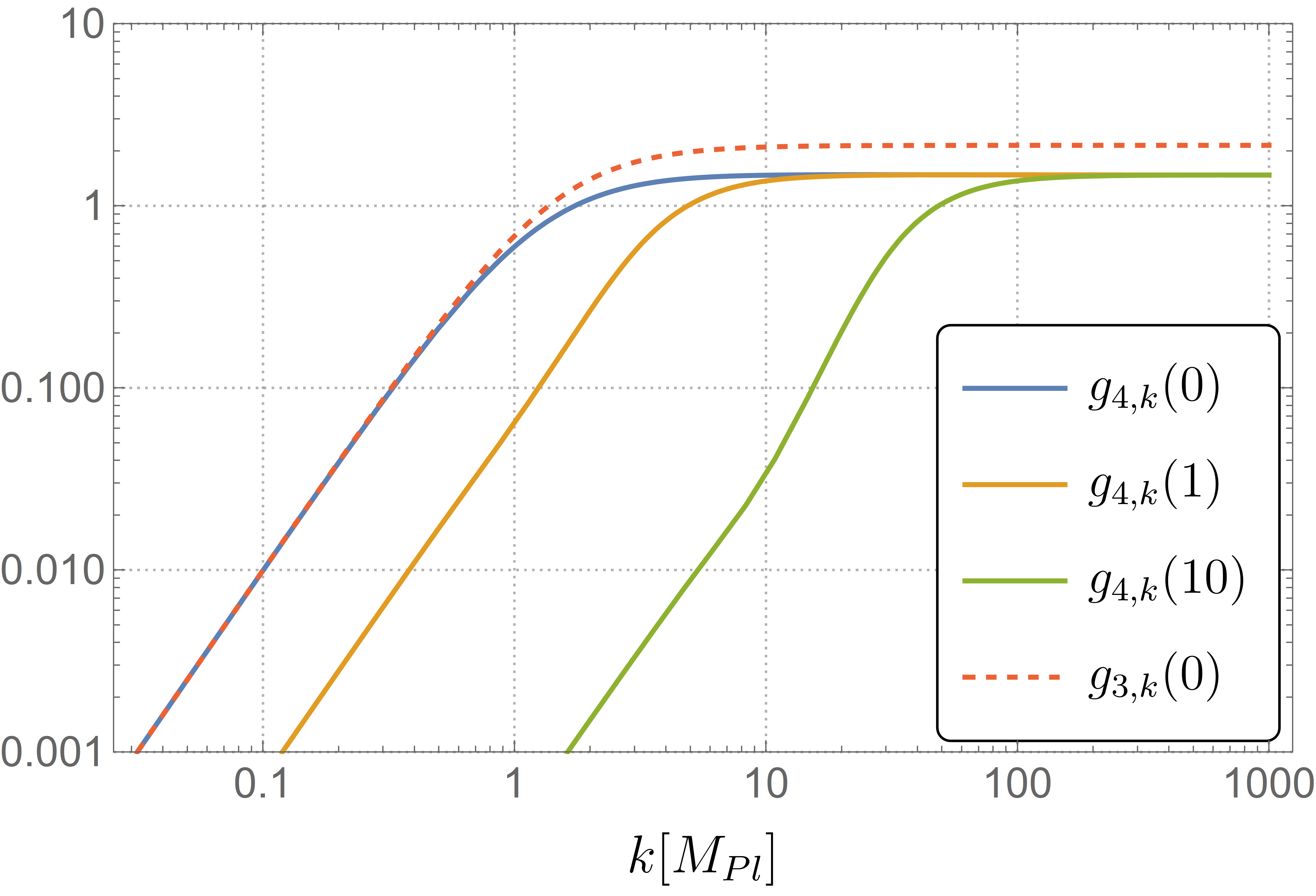
Figure 8: Examples of RG-trajectories $g_{4,k}(p)$ for different values of $p/M_{\text{Pl}}$. All scale canonically $\propto k^{2}$ below the Planck scale at $k=1$ and approach the fixed point value $g_{4}^{*}\approx 1.48$ in the UV. For reference $g_{3,k}(0)$ is also shown.

Some example trajectories are plotted in Figure 8. One can observe the canonical scaling $\propto k^{2}$ below the Planck scale at $k=1$. In the regime $k\gg 1$ all trajectories approach the UV fixed point $g_{4}^{*}$. For larger external momentum $p$ the asymptotically safe regime is reached at larger $k$, approximately when $k\gtrsim 10p$.

To obtain $\gamma_{h}^{(4)}(p)$ in the physical limit of vanishing cutoff $k\rightarrow 0$, we use 46 to transform back to the dimensionful coupling by multiplying the trajectories $g_{4,k}$ with $k^{-2}$. Upon doing this, the trajectories become constant in the IR and scale like $k^{-2}$ in the UV. Hence, we can simply read out the constant values in the IR, i.e. $k\rightarrow 0$, for each value of $p$. The resulting momentum dependent four-graviton coupling $\gamma_{h}^{(4)}(p)$ at vanishing cutoff is displayed in Figure 4.

Appendix F The generalized Einstein-Hilbert term

The dimensionless constant $\bar{\gamma}_{3}$ appearing in the definition 25 of $\mathcal{R}$ is defined by

$$\bar{\gamma}_{3}=\lim\limits_{p^{2}\to\infty}\left(\frac{\gamma_{g}^{(3)}(p^{2})}{p^{2}}\right)\,,$$ (63)

and its numerical value computed from our data is

$$\bar{\gamma}_{3}\approx 0.054\,.$$ (64)

As mentioned above, $\mathcal{R}$ contributes a term ${C_{\mathcal{R}}^{(n)}g_{\mathcal{R}}p^{2}}$ to the flow of the $n$-point functions $\bar{\Gamma}_{G}^{(n)}(p)$. In particular, for $n=3,4$ this contribution stems from the structure

$$R^{(n)}\left(\frac{\gamma_{g}^{(3)}-\bar{\gamma}_{3}\Delta}{\Delta+R}R\right)\Big{|}_{\Delta\rightarrow 0,R\rightarrow 0}\,.$$ (65)

Other derivative structures vanish due to our expansion about $R=0$ and the tt-projection. Because the field derivatives do not hit the term in brackets there is no associated momentum flow and $\Delta\rightarrow 0$ is taken before the evaluation at $h=0$ on the flat background with $R=0$.

This implies that the constant $g_{\mathcal{R}}$ which appears in the projected $\bar{\Gamma}_{G}^{(n)}(p)$ is given by ${g_{\mathcal{R}}=\gamma_{g}^{(3)}(0)=G_{N}^{-1}}$.

From 65 we further see that the $p^{2}$ contribution to the three- and four-point function generated by $\mathcal{R}$ has the same overlap with our parametrization as the tensor structures generated by $R$, i.e. ${C_{\mathcal{R}}=C_{R}}$ for $n=3,4$.

Appendix G Numerical values of couplings

The numerical values of the low energy couplings $g_{R_{\mu\nu}^{2}}$ and $g_{R^{2}}$ can be computed from our numerical data for $\gamma_{g}^{(3)}(p)$ and $\gamma_{g}^{(4)}(p)$ according to 28. Our construction results in the values

$$g_{R_{\mu\nu}^{2}}\approx-0.40\,,\qquad g_{R^{2}}\approx 1.9\,.$$ (66)

We note that $g_{R_{\mu\nu}^{2}}$ in our setup turns out to be negative, whereas $g_{R^{2}}$ is positive. The observational constraints on the couplings of higher curvature terms are still weak [74], such that our values are easily within the allowed region.

In the UV regime the form factors approach the values

$$\tilde{g}_{R_{\mu\nu}^{2}}\approx-0.023\,,\qquad\tilde{g}_{R^{2}}\approx 0.028\,.$$ (67)

The coefficients of the first order Taylor expansion 27 take the numerical values

$$c_{1}=-136.75\,,\quad c_{2}=344.09\,,$$ (68)

and

$$c_{3}=\frac{C_{R}^{(3)}}{C_{R_{\mu\nu}^{2}}^{(3)}}\,,\qquad c_{4}=\frac{C_{R}^{(4)}}{C_{R^{2}}^{(4)}}\,,\qquad c_{5}=\frac{C_{R_{\mu\nu}^{2}}^{(4)}}{C_{R^{2}}^{(4)}}\,c_{3}\,.$$ (69)

Since the seminal work [58] it is known that the spectrum of quadratic gravity, i.e. of an action containing $R+R^{2}+R_{\mu\nu}^{2}$ terms, in addition to the massless graviton contains a massive spin-two ghost and a massive spin-zero excitation with masses $m_{2}$ and $m_{0}$ respectively. With the values 66 of the couplings in our setup the masses are given by

$$m_{2}^{\phantom{2}2} =\frac{-G_{N}^{-1}}{g_{R_{\mu\nu}^{2}}}\approx 2.5\,M_{\text{pl}}^{2}\,,$$

$$m_{0}^{\phantom{0}2} =\frac{G_{N}^{-1}}{6g_{R^{2}}+2g_{R_{\mu\nu}^{2}}}\approx 0.095\,M_{\text{pl}}^{2}\,,$$ (70)

in units of the Planck mass. We note that, due to the signs and relative sizes of the couplings in 66, both masses turn out to be real and $m_{2}>m_{0}$.

Appendix H Analytic fits

Here we present analytic fits to the numerical data which could be used e.g. for phenomenological applications. Considering $\gamma_{h}^{(4)}(p)$, the simple expression

$$\gamma^{(4)}_{h,\text{simple}}(p^{2})=\frac{G_{4}^{*}}{G_{4}^{*}+p^{2}}\,,$$ (71)

with $G_{4}^{*}=0.0360$ captures the correct IR and UV asymptotes and could be used for applications in these limits. As a more elaborate model we use a Padé - type function

$$\gamma^{(4)}_{h,\text{fit}}(p^{2})=\frac{a_{1}+a_{2}p^{2}+a_{3}p^{4}+a_{4}p^{6}+a_{5}p^{8}}{b_{1}+b_{2}p^{2}+b_{3}p^{4}+b_{4}p^{6}+b_{5}p^{8}+b_{6}p^{10}}\,,$$ (72)

with free parameters $a_{i}$ and $b_{i}$. The best-fit values for this model are given by

$$a_{1} =0.0075542\,, \quad a_{2} =7.3967\,, \quad a_{3} =109.42\,,$$

$$a_{4} =122.40\,, \quad a_{5} =8.4140\,,$$

$$b_{1} =0.0075403\,, \quad b_{2} =7.4773\,, \quad b_{3} =153.00\,,$$

$$b_{4} =876.09\,, \quad b_{5} =2261.9\,, \quad b_{6} =228.87\,.$$ (73)

The fit describes the data well in the entire momentum range where numerical data is available with largest deviation from the data of $\sim 2\%$.

The best-fit values for the simple analytic model of the form factors 26 are given by

$$p_{0}\approx 0.27551\,,\quad p_{1}\approx-0.091916\,,$$ (74)

expressed in units of the Planck mass $p_{i}/M_{\text{Pl}}$. The Planck scale is defined dynamically by ${M_{\text{Pl}}^{2}\coloneqq\gamma_{g}^{(3)}(0)}$.

As a more elaborate fit function we employ

$$f_{R_{\mu\nu}^{2}\text{, fit}}(p^{2})=a_{0}+\displaystyle\sum_{i=1}^{4}\frac{a_{i}}{\left(p/p_{i}\right)^{2}+1}\,,$$ (75)

for $f_{R_{\mu\nu}^{2}}(p^{2})$ with best-fit values

$$a_{0} =-0.023601\,, \,a_{1} =-0.13727\,, \,a_{2} =0.13138\,,$$

$$a_{3} =-0.22100\,, \,a_{4} =-0.15080\,, \,p_{1} =0.12436\,,$$

$$p_{2} =1.2476\,, \,p_{3} =0.56405\,, \,p_{4} =0.021230\,.$$ (76)

For $f_{R^{2}}(p^{2})$ we use

$$f_{R^{2},\text{fit}}(p^{2})=a_{0}+\displaystyle\sum_{i=1}^{3}\frac{a_{i}}{\left(\left(p/p_{i}\right)^{2}+1\right)^{2}}\,,$$ (77)

with best-fit values given by

$$a_{0} =0.028373\,, \quad a_{1} =0.012637\,, \quad a_{2} =1.2661\,,$$

$$a_{3} =0.57040\,, \quad p_{1} =5.7131\,, \quad p_{2} =0.73200\,,$$

$$p_{3} =0.092956\,.$$ (78)

The fits describe the data to an accuracy of a few percent, with the largest deviations around $p\approx 1$.

References

- Weinberg [1980] S. Weinberg, Ultraviolet divergences in quantum theories of gravitation, in General Relativity: An Einstein Centenary Survey (1980) pp. 790–831.
- Reuter [1998] M. Reuter, Nonperturbative evolution equation for quantum gravity, Phys. Rev. D 57, 971 (1998), arXiv:hep-th/9605030 .
- Reuter and Saueressig [2019] M. Reuter and F. Saueressig, Quantum Gravity and the Functional Renormalization Group: The Road towards Asymptotic Safety (Cambridge University Press, 2019).
- Eichhorn [2020] A. Eichhorn, Asymptotically safe gravity, in 57th International School of Subnuclear Physics: In Search for the Unexpected (2020) arXiv:2003.00044 [gr-qc] .
- Bonanno et al. [2020] A. Bonanno, A. Eichhorn, H. Gies, J. M. Pawlowski, R. Percacci, M. Reuter, F. Saueressig, and G. P. Vacca, Critical reflections on asymptotically safe gravity, Front. in Phys. 8, 269 (2020), arXiv:2004.06810 [gr-qc] .
- Pawlowski and Reichert [2021] J. M. Pawlowski and M. Reichert, Quantum Gravity: A Fluctuating Point of View, Front. in Phys. 8, 551848 (2021), arXiv:2007.10353 [hep-th] .
- Christiansen et al. [2014] N. Christiansen, D. F. Litim, J. M. Pawlowski, and A. Rodigast, Fixed points and infrared completion of quantum gravity, Phys. Lett. B 728, 114 (2014), arXiv:1209.4038 [hep-th] .
- Christiansen et al. [2016] N. Christiansen, B. Knorr, J. M. Pawlowski, and A. Rodigast, Global Flows in Quantum Gravity, Phys. Rev. D 93, 044036 (2016), arXiv:1403.1232 [hep-th] .
- Christiansen et al. [2015] N. Christiansen, B. Knorr, J. Meibohm, J. M. Pawlowski, and M. Reichert, Local Quantum Gravity, Phys. Rev. D 92, 121501 (2015), arXiv:1506.07016 [hep-th] .
- Denz et al. [2018] T. Denz, J. M. Pawlowski, and M. Reichert, Towards apparent convergence in asymptotically safe quantum gravity, Eur. Phys. J. C 78, 336 (2018), arXiv:1612.07315 [hep-th] .
- Bonanno et al. [2022] A. Bonanno, T. Denz, J. M. Pawlowski, and M. Reichert, Reconstructing the graviton, SciPost Phys. 12, 001 (2022), arXiv:2102.02217 [hep-th] .
- Reichert [2020] M. Reichert, Lecture notes: Functional Renormalisation Group and Asymptotically Safe Quantum Gravity, PoS 384, 005 (2020).
- Fraaije et al. [2022] M. Fraaije, A. Platania, and F. Saueressig, On the reconstruction problem in quantum gravity, Phys. Lett. B 834, 137399 (2022), arXiv:2206.10626 [hep-th] .
- Koshelev et al. [2016] A. S. Koshelev, L. Modesto, L. Rachwal, and A. A. Starobinsky, Occurrence of exact inflation in non-local UV-complete gravity, JHEP 11, 067, arXiv:1604.03127 [hep-th] .
- Knorr and Saueressig [2018] B. Knorr and F. Saueressig, Towards reconstructing the quantum effective action of gravity, Phys. Rev. Lett. 121, 161304 (2018), arXiv:1804.03846 [hep-th] .
- Bosma et al. [2019] L. Bosma, B. Knorr, and F. Saueressig, Resolving Spacetime Singularities within Asymptotic Safety, Phys. Rev. Lett. 123, 101301 (2019), arXiv:1904.04845 [hep-th] .
- Knorr et al. [2019] B. Knorr, C. Ripken, and F. Saueressig, Form Factors in Asymptotic Safety: conceptual ideas and computational toolbox, Class. Quant. Grav. 36, 234001 (2019), arXiv:1907.02903 [hep-th] .
- Draper et al. [2020a] T. Draper, B. Knorr, C. Ripken, and F. Saueressig, Finite Quantum Gravity Amplitudes: No Strings Attached, Phys. Rev. Lett. 125, 181301 (2020a), arXiv:2007.00733 [hep-th] .
- Draper et al. [2020b] T. Draper, B. Knorr, C. Ripken, and F. Saueressig, Graviton-Mediated Scattering Amplitudes from the Quantum Effective Action, JHEP 11, 136, arXiv:2007.04396 [hep-th] .
- Knorr et al. [2022a] B. Knorr, C. Ripken, and F. Saueressig, Form Factors in Quantum Gravity: Contrasting non-local, ghost-free gravity and Asymptotic Safety, Nuovo Cim. C 45, 28 (2022a), arXiv:2111.12365 [hep-th] .
- Knorr and Schiffer [2021] B. Knorr and M. Schiffer, Non-Perturbative Propagators in Quantum Gravity, Universe 7, 216 (2021), arXiv:2105.04566 [hep-th] .
- Knorr and Platania [2022] B. Knorr and A. Platania, Sifting quantum black holes through the principle of least action, Phys. Rev. D 106, L021901 (2022), arXiv:2202.01216 [hep-th] .
- Platania and Redondo-Yuste [2023] A. Platania and J. Redondo-Yuste, Diverging black hole entropy from quantum infrared non-localities, (2023), arXiv:2303.17621 [hep-th] .
- Knorr et al. [2022b] B. Knorr, C. Ripken, and F. Saueressig, Form Factors in Asymptotically Safe Quantum Gravity, (2022b), arXiv:2210.16072 [hep-th] .
- Falls et al. [2016] K. Falls, D. F. Litim, K. Nikolakopoulos, and C. Rahmede, Further evidence for asymptotic safety of quantum gravity, Phys. Rev. D 93, 104022 (2016), arXiv:1410.4815 [hep-th] .
- Falls et al. [2019] K. G. Falls, D. F. Litim, and J. Schröder, Aspects of asymptotic safety for quantum gravity, Phys. Rev. D 99, 126015 (2019), arXiv:1810.08550 [gr-qc] .
- Baldazzi and Falls [2021] A. Baldazzi and K. Falls, Essential Quantum Einstein Gravity, Universe 7, 294 (2021), arXiv:2107.00671 [hep-th] .
- Christiansen [2016] N. Christiansen, Four-Derivative Quantum Gravity Beyond Perturbation Theory (2016) arXiv:1612.06223 [hep-th] .
- Dupuis et al. [2021] N. Dupuis, L. Canet, A. Eichhorn, W. Metzner, J. M. Pawlowski, M. Tissier, and N. Wschebor, The nonperturbative functional renormalization group and its applications, Phys. Rept. 910, 1 (2021), arXiv:2006.04853 [cond-mat.stat-mech] .
- Fu [2022] W.-j. Fu, QCD at finite temperature and density within the fRG approach: an overview, Commun. Theor. Phys. 74, 097304 (2022), arXiv:2205.00468 [hep-ph] .
- Eichhorn et al. [2018] A. Eichhorn, P. Labus, J. M. Pawlowski, and M. Reichert, Effective universality in quantum gravity, SciPost Phys. 5, 031 (2018), arXiv:1804.00012 [hep-th] .
- Eichhorn et al. [2019] A. Eichhorn, S. Lippoldt, J. M. Pawlowski, M. Reichert, and M. Schiffer, How perturbative is quantum gravity?, Phys. Lett. B 792, 310 (2019), arXiv:1810.02828 [hep-th] .
- Christiansen et al. [2018] N. Christiansen, K. Falls, J. M. Pawlowski, and M. Reichert, Curvature dependence of quantum gravity, Phys. Rev. D 97, 046007 (2018), arXiv:1711.09259 [hep-th] .
- Bürger et al. [2019] B. Bürger, J. M. Pawlowski, M. Reichert, and B.-J. Schaefer, Curvature dependence of quantum gravity with scalars (2019) arXiv:1912.01624 [hep-th] .
- Saueressig [2023] F. Saueressig, The Functional Renormalization Group in Quantum Gravity, (2023), arXiv:2302.14152 [hep-th] .
- Wetterich [1993] C. Wetterich, Exact evolution equation for the effective potential, Phys. Lett. B 301, 90 (1993), arXiv:1710.05815 [hep-th] .
- Bonanno and Reuter [2000] A. Bonanno and M. Reuter, Renormalization group improved black hole space-times, Phys. Rev. D 62, 043008 (2000), arXiv:hep-th/0002196 .
- Bonanno and Reuter [2006] A. Bonanno and M. Reuter, Spacetime structure of an evaporating black hole in quantum gravity, Phys. Rev. D 73, 083005 (2006), arXiv:hep-th/0602159 .
- Falls et al. [2012] K. Falls, D. F. Litim, and A. Raghuraman, Black Holes and Asymptotically Safe Gravity, Int. J. Mod. Phys. A 27, 1250019 (2012), arXiv:1002.0260 [hep-th] .
- Cai and Easson [2010] Y.-F. Cai and D. A. Easson, Black holes in an asymptotically safe gravity theory with higher derivatives, JCAP 09, 002, arXiv:1007.1317 [hep-th] .
- Becker and Reuter [2012] D. Becker and M. Reuter, Running boundary actions, Asymptotic Safety, and black hole thermodynamics, JHEP 07, 172, arXiv:1205.3583 [hep-th] .
- Falls and Litim [2014] K. Falls and D. F. Litim, Black hole thermodynamics under the microscope, Phys. Rev. D 89, 084002 (2014), arXiv:1212.1821 [gr-qc] .
- Koch and Saueressig [2014a] B. Koch and F. Saueressig, Structural aspects of asymptotically safe black holes, Class. Quant. Grav. 31, 015006 (2014a), arXiv:1306.1546 [hep-th] .
- Koch et al. [2016] B. Koch, C. Contreras, P. Rioseco, and F. Saueressig, Black holes and running couplings: A comparison of two complementary approaches, Springer Proc. Phys. 170, 263 (2016), arXiv:1311.1121 [hep-th] .
- Koch and Saueressig [2014b] B. Koch and F. Saueressig, Black holes within Asymptotic Safety, Int. J. Mod. Phys. A 29, 1430011 (2014b), arXiv:1401.4452 [hep-th] .
- Saueressig et al. [2016] F. Saueressig, N. Alkofer, G. D’Odorico, and F. Vidotto, Black holes in Asymptotically Safe Gravity, PoS FFP14, 174 (2016), arXiv:1503.06472 [hep-th] .
- Pawlowski and Stock [2018] J. M. Pawlowski and D. Stock, Quantum-improved Schwarzschild-(A)dS and Kerr-(A)dS spacetimes, Phys. Rev. D 98, 106008 (2018), arXiv:1807.10512 [hep-th] .
- Platania [2019] A. Platania, Dynamical renormalization of black-hole spacetimes, Eur. Phys. J. C 79, 470 (2019), arXiv:1903.10411 [gr-qc] .
- Borissova et al. [2022] J. N. Borissova, A. Held, and N. Afshordi, Scale-Invariance at the Core of Quantum Black Holes (2022) (2022), arXiv:2203.02559 [gr-qc] .
- Chen et al. [2022] C.-M. Chen, Y. Chen, A. Ishibashi, N. Ohta, and D. Yamaguchi, Running Newton coupling, scale identification, and black hole thermodynamics, Phys. Rev. D 105, 106026 (2022), arXiv:2204.09892 [hep-th] .
- Bonanno et al. [2023] A. Bonanno, D. Malafarina, and A. Panassiti, Dust collapse in asymptotic safety: a path to regular black holes, (2023), arXiv:2308.10890 [gr-qc] .
- Platania [2023] A. Platania, Black Holes in Asymptotically Safe Gravity, (2023), arXiv:2302.04272 [gr-qc] .
- Held [2021] A. Held, Invariant Renormalization-Group improvement, (2021), arXiv:2105.11458 [gr-qc] .
- Manrique et al. [2011] E. Manrique, S. Rechenberger, and F. Saueressig, Asymptotically Safe Lorentzian Gravity, Phys. Rev. Lett. 106, 251302 (2011), arXiv:1102.5012 [hep-th] .
- Candelas and Raine [1977] P. Candelas and D. J. Raine, Feynman Propagator in Curved Space-Time, Phys. Rev. D 15, 1494 (1977).
- Visser [2017] M. Visser, How to Wick rotate generic curved spacetime, (2017), arXiv:1702.05572 [gr-qc] .
- Baldazzi et al. [2019] A. Baldazzi, R. Percacci, and V. Skrinjar, Wicked metrics, Class. Quant. Grav. 36, 105008 (2019), arXiv:1811.03369 [gr-qc] .
- Stelle [1978] K. S. Stelle, Classical Gravity with Higher Derivatives, Gen. Rel. Grav. 9, 353 (1978).
- Antonsen and Bormann [1996] F. Antonsen and K. Bormann, Propagators in curved space (1996) arXiv:hep-th/9608141 .
- Lü et al. [2015a] H. Lü, A. Perkins, C. N. Pope, and K. S. Stelle, Black Holes in Higher-Derivative Gravity, Phys. Rev. Lett. 114, 171601 (2015a), arXiv:1502.01028 [hep-th] .
- Lü et al. [2015b] H. Lü, A. Perkins, C. N. Pope, and K. S. Stelle, Spherically Symmetric Solutions in Higher-Derivative Gravity, Phys. Rev. D 92, 124019 (2015b), arXiv:1508.00010 [hep-th] .
- Holdom and Ren [2017] B. Holdom and J. Ren, Not quite a black hole, Phys. Rev. D 95, 084034 (2017), arXiv:1612.04889 [gr-qc] .
- Podolsky et al. [2018] J. Podolsky, R. Svarc, V. Pravda, and A. Pravdova, Explicit black hole solutions in higher-derivative gravity, Phys. Rev. D 98, 021502 (2018), arXiv:1806.08209 [gr-qc] .
- Goldstein and Mashiyane [2018] K. Goldstein and J. J. Mashiyane, Ineffective Higher Derivative Black Hole Hair, Phys. Rev. D 97, 024015 (2018), arXiv:1703.02803 [hep-th] .
- Bonanno and Silveravalle [2019] A. Bonanno and S. Silveravalle, Characterizing black hole metrics in quadratic gravity, Phys. Rev. D 99, 101501 (2019), arXiv:1903.08759 [gr-qc] .
- Podolský et al. [2020] J. Podolský, R. Švarc, V. Pravda, and A. Pravdova, Black holes and other exact spherical solutions in Quadratic Gravity, Phys. Rev. D 101, 024027 (2020), arXiv:1907.00046 [gr-qc] .
- Saueressig et al. [2021] F. Saueressig, M. Galis, J. Daas, and A. Khosravi, Asymptotically flat black hole solutions in quadratic gravity, Int. J. Mod. Phys. D 30, 2142015 (2021).
- Daas et al. [2022] J. Daas, K. Kuijpers, F. Saueressig, M. F. Wondrak, and H. Falcke, Probing Quadratic Gravity with the Event Horizon Telescope (2022) arXiv:2204.08480 [gr-qc] .
- Silveravalle and Zuccotti [2022] S. Silveravalle and A. Zuccotti, The phase diagram of Einstein-Weyl gravity, (2022), arXiv:2210.13877 [gr-qc] .
- Meibohm et al. [2016] J. Meibohm, J. M. Pawlowski, and M. Reichert, Asymptotic safety of gravity-matter systems, Phys. Rev. D 93, 084035 (2016), arXiv:1510.07018 [hep-th] .
- Stelle [1977] K. S. Stelle, Renormalization of Higher Derivative Quantum Gravity, Phys. Rev. D 16, 953 (1977).
- Wolfram Research (2019) [1991] Wolfram Research (1991), NDSolve - wolfram language function, https://reference.wolfram.com/language/ref/NDSolve.html (2019).
- Litim [2001] D. F. Litim, Optimized renormalization group flows, Phys. Rev. D 64, 105007 (2001), arXiv:hep-th/0103195 .
- Berry and Gair [2011] C. P. L. Berry and J. R. Gair, Linearized f(R) Gravity: Gravitational Radiation and Solar System Tests, Phys. Rev. D 83, 104022 (2011), [Erratum: Phys.Rev.D 85, 089906 (2012)], arXiv:1104.0819 [gr-qc] .