Computing singular and near-singular integrals over curved boundary elements: The strongly singular case

Abstract

We present algorithms for computing strongly singular and near-singular surface integrals over curved triangular patches, based on singularity subtraction, the continuation approach, and transplanted Gauss quadrature. We demonstrate the accuracy and robustness of our method for quadratic basis functions and quadratic triangles by integrating it into a boundary element code and solving several scattering problems in 3D. We also give numerical evidence that the utilization of curved boundary elements enhances computational efficiency compared to conventional planar elements.

35J05, 41A55, 41A58, 45E05, 45E99, 65N38, 65R20, 78M15

1 Introduction

The Helmholtz equation, which has the form

(1) $$\Delta u+k^{2}u=0,$$

appears when one looks for time-harmonic solutions to the wave equation—if $v(\boldsymbol{x},t)=u(\boldsymbol{x})e^{-i\omega t}$ is a solution to $v_{tt}=c^{2}\Delta v$, then $u$ satisfies Eq. 1 with wavenumber $k=\omega/c$. It is of fundamental importance in science and engineering, with applications as diverse as noise scattering, radar and sonar technology, and seismology. For instance, given an incident acoustic wave $u^{i}$ that is a solution to Eq. 1 in $\mathbb{R}^{3}$, the outgoing scattered field $u^{s}$ generated by a bounded obstacle $D$ is also a solution to Eq. 1, in $\mathbb{R}^{3}\setminus\overline{D}$, with $u^{i}+u^{s}=0$ on the boundary $\partial D$ (for sound-soft scattering).

For obstacles $D$ whose complements are connected, a popular technique for calculating scattered fields is based on integral equations. As an example, one can show that the solution $u^{s}$ to the sound-soft scattering problem of the previous paragraph may be obtained by solving [4, eq. (3.51)],

(2) $$\int_{\partial D}\left\{\frac{\partial G(\boldsymbol{x},\boldsymbol{y})}{\partial\boldsymbol{n}(\boldsymbol{y})}-i\eta G(\boldsymbol{x},\boldsymbol{y})\right\}\varphi^{s}(\boldsymbol{y})dS(\boldsymbol{y})+\frac{\varphi^{s}(\boldsymbol{x})}{2}=-u^{i}(\boldsymbol{x}),\quad\boldsymbol{x}\in\partial D,$$

for some arbitrary real number $\eta\neq 0$ such that $\eta\mathrm{Re}(k)\geq 0$. (The solution to Eq. 2 is unique when $\mathrm{Im}\,k\geq 0$ [4, Thm. 3.33].) Once Eq. 2 is solved for $\varphi^{s}$, the scattered field is given by [4, eq. (3.49)]

(3) $$u^{s}(\boldsymbol{x})=\int_{\partial D}\left\{\frac{\partial G(\boldsymbol{x},\boldsymbol{y})}{\partial\boldsymbol{n}(\boldsymbol{y})}-i\eta G(\boldsymbol{x},\boldsymbol{y})\right\}\varphi^{s}(\boldsymbol{y})dS(\boldsymbol{y}),\quad\boldsymbol{x}\in\mathbb{R}^{3}\setminus{\overline{D}}.$$

The function $G$ in Eq. 2 and Eq. 3 is the Green’s function of the Helmholtz equation in 3D,

(4) $$G(\boldsymbol{x},\boldsymbol{y})=\frac{1}{4\pi}\frac{e^{ik|\boldsymbol{x}-\boldsymbol{y}|}}{|\boldsymbol{x}-\boldsymbol{y}|}.$$

One of the challenges one faces when solving integral equations of the form of Eq. 2 is the computation of singular integrals—when $\boldsymbol{x}$ is close or equal to $\boldsymbol{y}$, the Green’s function and its derivatives become (numerically) unbounded. There are many specialized methods to compute such integrals, including singularity subtraction [1, 9, 10, 12], singularity cancellation [6, 13, 20, 21], and the continuation approach [15, 22, 23, 26, 30]. Recent works include [7, 14, 19, 32].

We proposed, in a previous paper, algorithms to compute weakly singular integrals using singularity subtraction and the continuation approach [17]. The term weakly singular refers to integrals with singularities of the same type as the Green’s function Eq. 4. We extend, here, our method to strongly singular integrals, which have singularities of the same nature as the derivatives of Eq. 4. Specifically, we consider strongly singular and near-singular integrals of the form

(5) $$I(\boldsymbol{x}_{0})=\int_{\mathcal{T}}\frac{(\boldsymbol{x}-\boldsymbol{x}_{0})\cdot\boldsymbol{n}(\boldsymbol{x})}{|\boldsymbol{x}-\boldsymbol{x}_{0}|^{3}}\varphi(F^{-1}(\boldsymbol{x}))dS(\boldsymbol{x}),$$

where $\mathcal{T}\subset\mathbb{R}^{3}$ is a curved triangle defined by a polynomial transformation $F:\widehat{T}\to\mathcal{T}$ of degree $q\geq 1$ from some reference planar triangle $\widehat{T}\subset\mathbb{R}^{2}$, $\boldsymbol{x}_{0}\in\mathbb{R}^{3}$ is a point on/or close to $\mathcal{T}$, $\varphi:\widehat{T}\to\mathbb{R}$ is a polynomial function of degree $p\geq 0$ (not necessarily equal to $q$), and $\boldsymbol{n}(\boldsymbol{x})$ is the unit normal vector at $\boldsymbol{x}$. As in the companion paper [17], our method is based on the computation of the preimage of the singularity in the reference element’s space using Newton’s method, singularity subtraction with Taylor-like asymptotic expansions, the continuation approach, and transplanted Gauss quadrature. Integrals of the form of Eq. 5 appear when evaluating the solution Eq. 3 at $\boldsymbol{x}_{0}$—we will also look at integrals over two triangles, which occur when solving Eq. 2 with a boundary element method [27].

One of the main advantages of our method over the standard continuation approach [23] is that we perform singularity subtraction and continuation after mapping back to the reference triangle, which is both computationally less expensive and much easier to implement. Our novel algorithms are also particularly well-suited for configurations where the singularity is close to the patch’s edges. Finally, the benefit of being able to compute strong singularities is that we can solve the Dirichlet problem using the combined boundary integral equation Eq. 2, which is coercive when $k$ is large [28]. (Coercivity gives explicit bounds one the number of GMRES iterations to achieve a given accuracy.) Our previous work was limited to weak singularities and the (inferior) single-layer formulation.

We start by reviewing the properties of the solid angle in Section 2, which is closely connected to the strongly singular and near-singular integrals Eq. 5. We then present our method for computing such integrals in Section 3, and provide several numerical examples in Section 4.

2 The solid angle

When $\varphi$ is the constant function $1$, the integral Eq. 5 simplifies to

(6) $$I(\boldsymbol{x}_{0})=\int_{\mathcal{T}}\frac{(\boldsymbol{x}-\boldsymbol{x}_{0})\cdot\boldsymbol{n}(\boldsymbol{x})}{|\boldsymbol{x}-\boldsymbol{x}_{0}|^{3}}dS(\boldsymbol{x})=-\Omega(\boldsymbol{x}_{0}),$$

where $\Omega(\boldsymbol{x}_{0})$ is the solid angle of the curved triangle $\mathcal{T}$ subtended at the point $\boldsymbol{x}_{0}$. The solid angle $\Omega(\boldsymbol{x}_{0})$ cannot be expressed using a closed-form formula for a general curved triangle of degree $q\geq 2$. However, in the case of planar triangles where $q=1$, a closed-form formula does exist, which we will examine next to highlight some of the key features of strongly singular integrals.

2.1 Planar triangles

Figure 1: An arbitrary planar triangle $\mathcal{T}$ is obtained from the planar reference triangle $\widehat{T}$ via the linear map $F$ defined in Eq. 8. The $\boldsymbol{\hat{a}}_{j}$’s verify $\lambda_{i}(\boldsymbol{\hat{a}}_{j})=\delta_{ij}$, while the $\boldsymbol{a}_{j}$’s verify $\boldsymbol{a}_{j}=F(\boldsymbol{\hat{a}}_{j})$.

Let $\widehat{T}$ be the reference planar triangle,

(7) $$\widehat{T}=\{(\hat{x}_{1},\hat{x}_{2})\,:\,0\leq\hat{x}_{1}\leq 1,\;0\leq\hat{x}_{2}\leq 1-\hat{x}_{1}\}\subset\mathbb{R}^{2}.$$

An arbitrary planar triangle $\mathcal{T}\subset\mathbb{R}^{3}$ may be defined by three points $\boldsymbol{a}_{j}\in\mathbb{R}^{3}$ and a linear transformation $F:\widehat{T}\mapsto\mathcal{T}$,

(8) $$F(\boldsymbol{\hat{x}})=\sum_{j=1}^{3}\lambda_{j}(\boldsymbol{\hat{x}})\boldsymbol{a}_{j}\in\mathbb{R}^{3},$$

with $\boldsymbol{\hat{x}}=(\hat{x}_{1},\hat{x}_{2})$, and where the $\lambda_{j}$’s are the linear basis functions defined on $\widehat{T}$ by

(9) $$\lambda_{1}(\boldsymbol{\hat{x}})=1-\hat{x}_{1}-\hat{x}_{2},\quad\lambda_{2}(\boldsymbol{\hat{x}})=\hat{x}_{1},\quad\lambda_{3}(\boldsymbol{\hat{x}})=\hat{x}_{2}.$$

We illustrate this in Fig. 1. Note that $F(\boldsymbol{\hat{x}})=J\boldsymbol{\hat{x}}+\boldsymbol{a}_{1}$ with a constant Jacobian matrix

(13) $$J=\left(\begin{array}[]{c|c}&\\ \boldsymbol{a}_{2}-\boldsymbol{a}_{1}&\boldsymbol{a}_{3}-\boldsymbol{a}_{1}\\ &\end{array}\right)\in\mathbb{R}^{3\times 2}.$$

For such a triangle, the solid angle

(14) $$\Omega(\boldsymbol{x}_{0})=\int_{\mathcal{T}}\frac{(\boldsymbol{x}_{0}-\boldsymbol{x})\cdot\boldsymbol{n}}{|\boldsymbol{x}-\boldsymbol{x}_{0}|^{3}}dS(\boldsymbol{x}),\quad\boldsymbol{n}=\frac{(\boldsymbol{a}_{2}-\boldsymbol{a}_{1})\times(\boldsymbol{a}_{3}-\boldsymbol{a}_{2})}{|(\boldsymbol{a}_{2}-\boldsymbol{a}_{1})\times(\boldsymbol{a}_{3}-\boldsymbol{a}_{2})|},$$

may be computed via the following formula [29],

(15) $$\Omega(\boldsymbol{x}_{0})=\mathrm{sign}((\boldsymbol{x}_{0}-\boldsymbol{a}_{1})\cdot\boldsymbol{n})\times(-\pi+\phi_{1}(\boldsymbol{x}_{0})+\phi_{2}(\boldsymbol{x}_{0})+\phi_{3}(\boldsymbol{x}_{0})),$$

with dihedral angles

(16) $$\phi_{1}=\mathrm{acos}\left(\frac{c_{1}-c_{2}c_{3}}{s_{2}s_{3}}\right),\quad\phi_{2}=\mathrm{acos}\left(\frac{c_{2}-c_{1}c_{3}}{s_{1}s_{3}}\right),\quad\phi_{3}=\mathrm{acos}\left(\frac{c_{3}-c_{1}c_{2}}{s_{1}s_{2}}\right).$$

The $c_{i}$’s above are given by

(17) $$c_{1}=\frac{(\boldsymbol{a}_{2}-\boldsymbol{x}_{0})\cdot(\boldsymbol{a}_{3}-\boldsymbol{x}_{0})}{\big{|}\boldsymbol{a}_{2}-\boldsymbol{x}_{0}\big{|}\big{|}\boldsymbol{a}_{3}-\boldsymbol{x}_{0}\big{|}},\quad c_{2}=\frac{(\boldsymbol{a}_{1}-\boldsymbol{x}_{0})\cdot(\boldsymbol{a}_{3}-\boldsymbol{x}_{0})}{\big{|}\boldsymbol{a}_{1}-\boldsymbol{x}_{0}\big{|}\big{|}\boldsymbol{a}_{3}-\boldsymbol{x}_{0}\big{|}},\quad c_{3}=\frac{(\boldsymbol{a}_{1}-\boldsymbol{x}_{0})\cdot(\boldsymbol{a}_{2}-\boldsymbol{x}_{0})}{\big{|}\boldsymbol{a}_{1}-\boldsymbol{x}_{0}\big{|}\big{|}\boldsymbol{a}_{2}-\boldsymbol{x}_{0}\big{|}},$$

while the $s_{i}$’s are given by $s_{i}=\sqrt{1-c_{i}^{2}}$.

An important consequence of Eq. 15 is that, as $\boldsymbol{x}_{0}$ approaches the interior of $\mathcal{T}$ from above (with respect to its normal), $\Omega(\boldsymbol{x}_{0})$ tends to $2\pi$, since each of the dihedral angles tends to $\pi$. On the other hand, when $\boldsymbol{x}_{0}$ approaches an edge or the vertex $\boldsymbol{a}_{i}$ of $\mathcal{T}$, $\Omega(\boldsymbol{x}_{0})$ tends to $\pi$ or to the dihedral angle $\phi_{i}$, respectively. Finally, $\Omega(\boldsymbol{x}_{0})$ goes to $0$ when $\boldsymbol{x}_{0}$ approaches a point in the plane of $\mathcal{T}$ while staying outside of $\mathcal{T}$. (These results have to be changed to their negatives if $\boldsymbol{x}_{0}$ approaches $\mathcal{T}$ from below.) To summarize, we have the following limits:

(18) $$\Omega(\boldsymbol{x}_{0})\to\pm 2\pi, \text{as $\boldsymbol{x}_{0}$ approaches the interior of $\mathcal{T}$},$$

$$\Omega(\boldsymbol{x}_{0})\to\pm\pi, \text{as $\boldsymbol{x}_{0}$ approaches an edge of $\mathcal{T}$ but not a vertex},$$

$$\Omega(\boldsymbol{x}_{0})\to\pm\phi_{i}, \text{as $\boldsymbol{x}_{0}$ approaches the vertex $\boldsymbol{a}_{i}$ of $\mathcal{T}$},$$

$$\Omega(\boldsymbol{x}_{0})\to 0, \text{as $\boldsymbol{x}_{0}$ approaches the exterior $\mathcal{T}$}.$$

Therefore, the solid angle is discontinuous through $\mathcal{T}$ but, in view of Eq. 18, we may set

(19) $$\Omega(\boldsymbol{x}_{0})=\frac{\lim_{\boldsymbol{x}_{0}\to\mathcal{T}^{+}}\Omega(\boldsymbol{x}_{0})+\lim_{\boldsymbol{x}_{0}\to\mathcal{T}^{-}}\Omega(\boldsymbol{x}_{0})}{2}=0,\quad\boldsymbol{x}_{0}\in\mathcal{T}.$$

(In this formula, $\mathcal{T}^{\pm}$ means that the point $\boldsymbol{x}_{0}$ approaches the triangle $\mathcal{T}$ from above/below.)

Another way to obtain the limits Eq. 18, which will be useful for curved triangles, is to map the solid angle back to the reference triangle $\widehat{T}$,

(20) $$\Omega(\boldsymbol{x}_{0})=\int_{\widehat{T}}\frac{(\boldsymbol{x}_{0}-F(\boldsymbol{\hat{x}}))\cdot\boldsymbol{\hat{n}}}{|F(\boldsymbol{\hat{x}})-\boldsymbol{x}_{0}|^{3}}dS(\boldsymbol{\hat{x}}),\quad\boldsymbol{\hat{n}}=J_{1}\times J_{2},$$

and write $\boldsymbol{x}_{0}$ as the sum of a vector parallel to $\mathcal{T}$ and a vector orthogonal to $\mathcal{T}$,

(21) $$\boldsymbol{x}_{0}=F(\boldsymbol{\hat{x}}_{0})+h\frac{\boldsymbol{\hat{n}}}{|\boldsymbol{\hat{n}}|},$$

for some scalar $h$. Using $F(\boldsymbol{\hat{x}})=J\boldsymbol{\hat{x}}+\boldsymbol{a}_{1}$, we get $\Omega(\boldsymbol{\hat{x}}_{0},h)=\Omega_{-1}(\boldsymbol{\hat{x}}_{0},h)+\Omega_{-2}(\boldsymbol{\hat{x}}_{0},h)$ with

(22) $$\Omega_{-1}(\boldsymbol{\hat{x}}_{0},h)=\int_{\widehat{T}}\frac{\left[J(\boldsymbol{\hat{x}}_{0}-\boldsymbol{\hat{x}})\right]\cdot\boldsymbol{\hat{n}}}{\left[|J(\boldsymbol{\hat{x}}-\boldsymbol{\hat{x}}_{0})|^{2}+h^{2}\right]^{\frac{3}{2}}}dS(\boldsymbol{\hat{x}}),$$

$$\Omega_{-2}(\boldsymbol{\hat{x}}_{0},h)=\int_{\widehat{T}}\frac{h|\boldsymbol{\hat{n}}|}{\left[|J(\boldsymbol{\hat{x}}-\boldsymbol{\hat{x}}_{0})|^{2}+h^{2}\right]^{\frac{3}{2}}}dS(\boldsymbol{\hat{x}}).$$

The term $\Omega_{-1}(\boldsymbol{\hat{x}}_{0},h)$ vanishes for all $\boldsymbol{\hat{x}}_{0}$ and $h$ since $J(\boldsymbol{\hat{x}}_{0}-\boldsymbol{\hat{x}})$ is orthogonal to the normal $\boldsymbol{\hat{n}}$. The term $\Omega_{-2}(\boldsymbol{\hat{x}}_{0},h)$ is strongly singular and we recover the limits Eq. 18 by noting that the integrand approaches the radially symmetric Dirac delta as $h\to 0^{\pm}$. In other words, we have

(23) $$\Omega(\boldsymbol{\hat{x}}_{0},h)=\int_{\widehat{T}}\frac{h|\boldsymbol{\hat{n}}|}{\left[|J(\boldsymbol{\hat{x}}-\boldsymbol{\hat{x}}_{0})|^{2}+h^{2}\right]^{\frac{3}{2}}}dS(\boldsymbol{\hat{x}}),$$

with the limits

(24) $$\lim_{h\to 0^{\pm}}\Omega(\boldsymbol{\hat{x}}_{0},h)\to\pm 2\pi, \text{if $\boldsymbol{\hat{x}}_{0}$ is in the interior of $\widehat{T}$},$$

$$\lim_{h\to 0^{\pm}}\Omega(\boldsymbol{\hat{x}}_{0},h)\to\pm\pi, \text{if $\boldsymbol{\hat{x}}_{0}$ is on an edge of $\widehat{T}$ but is not a vertex},$$

$$\lim_{h\to 0^{\pm}}\Omega(\boldsymbol{\hat{x}}_{0},h)\to\pm\phi_{i}, \text{if $\boldsymbol{\hat{x}}_{0}$ is a vertex of $\widehat{T}$, that is, $F(\boldsymbol{\hat{x}}_{0})=\boldsymbol{a}_{i}$},$$

$$\lim_{h\to 0^{\pm}}\Omega(\boldsymbol{\hat{x}}_{0},h)\to 0, \text{if $\boldsymbol{\hat{x}}_{0}$ is in the exterior $\widehat{T}$}.$$

Once again, we observe that $\Omega(\boldsymbol{\hat{x}}_{0},h)$ is discontinuous at $h=0$ but, in view of Eq. 24, we may set

(25) $$\Omega(\boldsymbol{\hat{x}}_{0},0)=0,\quad\boldsymbol{\hat{x}}_{0}\in\widehat{T}.$$

We summarize the limits Eq. 24 and Eq. 25 in Table 1. We may be tempted to say that the solid angle is merely weakly singular because of the cancellation when $h=0$. However, in practice, it will act as if it were strongly singular when $h$ is small. We will come back to this in Section 4.

Table 1: Limiting values of the solid angle $\Omega(\boldsymbol{\hat{x}}_{0},h)$ for planar triangles.

$h\to 0^{+}$	$h\to 0^{-}$	$h=0$

2.2 Curved triangles

Throughout the paper, we will utilize quadratic triangles to illustrate our results for curved triangles. A quadratic triangle $\mathcal{T}\subset\mathbb{R}^{3}$ may be defined by six points $\boldsymbol{a}_{j}\in\mathbb{R}^{3}$ and a quadratic map $F:\widehat{T}\to\mathcal{T}$,

(26) $$F(\boldsymbol{\hat{x}})=\sum_{j=1}^{6}\varphi_{j}(\boldsymbol{\hat{x}})\boldsymbol{a}_{j}\in\mathbb{R}^{3},$$

where the $\varphi_{j}$’s are the quadratic basis functions defined on $\widehat{T}$ by

(27) $$\varphi_{1}(\boldsymbol{\hat{x}})=\lambda_{1}(\boldsymbol{\hat{x}})(2\lambda_{1}(\boldsymbol{\hat{x}})-1),\quad\quad\varphi_{4}(\boldsymbol{\hat{x}})=4\lambda_{1}(\boldsymbol{\hat{x}})\lambda_{2}(\boldsymbol{\hat{x}}),$$

$$\varphi_{2}(\boldsymbol{\hat{x}})=\lambda_{2}(\boldsymbol{\hat{x}})(2\lambda_{2}(\boldsymbol{\hat{x}})-1),\quad\quad\varphi_{5}(\boldsymbol{\hat{x}})=4\lambda_{2}(\boldsymbol{\hat{x}})\lambda_{3}(\boldsymbol{\hat{x}}),$$

$$\varphi_{3}(\boldsymbol{\hat{x}})=\lambda_{3}(\boldsymbol{\hat{x}})(2\lambda_{3}(\boldsymbol{\hat{x}})-1),\quad\quad\varphi_{6}(\boldsymbol{\hat{x}})=4\lambda_{1}(\boldsymbol{\hat{x}})\lambda_{3}(\boldsymbol{\hat{x}}),$$

and the $\lambda_{j}$’s are defined in Eq. 9. We illustrate this in Fig. 2. Here, the Jacobian matrix $J$ reads

(31) $$J(\boldsymbol{\hat{x}})=\left(\begin{array}[]{c|c}&\\ F_{\hat{x}_{1}}(\boldsymbol{\hat{x}})&F_{\hat{x}_{2}}(\boldsymbol{\hat{x}})\phantom{}\\ &\end{array}\right)\in\mathbb{R}^{3\times 2},$$

with (componentwise) partial derivatives $F_{\hat{x}_{1}}(\boldsymbol{\hat{x}})\in\mathbb{R}^{3}$ and $F_{\hat{x}_{2}}(\boldsymbol{\hat{x}})\in\mathbb{R}^{3}$ with respect to $\hat{x}_{1}$ and $\hat{x}_{2}$.

Figure 2: A quadratic triangle $\mathcal{T}$ is obtained from $\widehat{T}$ via the quadratic map $F$ Eq. 26. Note that $\boldsymbol{\hat{a}}_{4}$, $\boldsymbol{\hat{a}}_{5}$, and $\boldsymbol{\hat{a}}_{6}$ are the midpoints. Again, the $\boldsymbol{\hat{a}}_{j}$’s verify $\varphi_{i}(\boldsymbol{\hat{a}}_{j})=\delta_{ij}$, while the $\boldsymbol{a}_{j}$’s verify $\boldsymbol{a}_{j}=F(\boldsymbol{\hat{a}}_{j})$.

Similarly to what we did for planar triangles, we may write the solid angle as

(32) $$\Omega(\boldsymbol{x}_{0})=\int_{\widehat{T}}\frac{(\boldsymbol{x}_{0}-F(\boldsymbol{\hat{x}}))\cdot\boldsymbol{\hat{n}}(\boldsymbol{\hat{x}})}{|F(\boldsymbol{\hat{x}})-\boldsymbol{x}_{0}|^{3}}dS(\boldsymbol{\hat{x}}),\quad\boldsymbol{\hat{n}}(\boldsymbol{\hat{x}})=F_{\hat{x}_{1}}(\boldsymbol{\hat{x}})\times F_{\hat{x}_{2}}(\boldsymbol{\hat{x}}),$$

and decompose $\boldsymbol{x}_{0}$ as the sum of a vector parallel to the tangent plane to the triangle $\mathcal{T}$ at $F(\boldsymbol{\hat{x}}_{0})$ and a vector orthogonal to that plane,

(33) $$\boldsymbol{x}_{0}=F(\boldsymbol{\hat{x}}_{0})+h\frac{\boldsymbol{\hat{n}}_{0}}{|\boldsymbol{\hat{n}}_{0}|},\quad\boldsymbol{\hat{n}}_{0}=\boldsymbol{\hat{n}}(\boldsymbol{\hat{x}}_{0}).$$

This yields $\Omega(\boldsymbol{\hat{x}}_{0},h)=\Omega_{-1}(\boldsymbol{\hat{x}}_{0},h)+\Omega_{-2}(\boldsymbol{\hat{x}}_{0},h)$ with

(34) $$\Omega_{-1}(\boldsymbol{\hat{x}}_{0},h)=\int_{\widehat{T}}\frac{(F(\boldsymbol{\hat{x}}_{0})-F(\boldsymbol{\hat{x}}))\cdot\boldsymbol{\hat{n}}(\boldsymbol{\hat{x}})}{|F(\boldsymbol{\hat{x}})-F(\boldsymbol{\hat{x}}_{0})-h\boldsymbol{\hat{n}}_{0}/|\boldsymbol{\hat{n}}_{0}||^{3}}dS(\boldsymbol{\hat{x}}),$$

$$\Omega_{-2}(\boldsymbol{\hat{x}}_{0},h)=\int_{\widehat{T}}\frac{h\boldsymbol{\hat{n}}_{0}/|\boldsymbol{\hat{n}}_{0}|\cdot\boldsymbol{\hat{n}}(\boldsymbol{\hat{x}})}{|F(\boldsymbol{\hat{x}})-F(\boldsymbol{\hat{x}}_{0})-h\boldsymbol{\hat{n}}_{0}/|\boldsymbol{\hat{n}}_{0}||^{3}}dS(\boldsymbol{\hat{x}}).$$

The term $\Omega_{-1}(\boldsymbol{\hat{x}}_{0},h)$ is weakly singular, continuous at $h=0$, and does not vanish in general, while the term $\Omega_{-2}(\boldsymbol{\hat{x}}_{0},h)$ is strongly singular, discontinuous at $h=0$, and has the same limits as Eq. 24. This can be shown by nothing that

(35) $$\int_{\widehat{T}}\frac{h\boldsymbol{\hat{n}}_{0}/|\boldsymbol{\hat{n}}_{0}|\cdot\boldsymbol{\hat{n}}(\boldsymbol{\hat{x}})}{|F(\boldsymbol{\hat{x}})-F(\boldsymbol{\hat{x}}_{0})-h\boldsymbol{\hat{n}}_{0}/|\boldsymbol{\hat{n}}_{0}||^{3}}dS(\boldsymbol{\hat{x}})=\int_{\widehat{T}}\frac{h|\boldsymbol{\hat{n}}_{0}|}{\left[|J_{0}(\boldsymbol{\hat{x}}-\boldsymbol{\hat{x}}_{0})|^{2}+h^{2}\right]^{\frac{3}{2}}}dS(\boldsymbol{\hat{x}})+\mathcal{O}(h),$$

where $J_{0}=J(\boldsymbol{\hat{x}}_{0})$. Again, we may set $\Omega_{-2}(\boldsymbol{\hat{x}}_{0},0)=0$ for all $\boldsymbol{\hat{x}}_{0}\in\widehat{T}$; see Table 2. The solid angle is mathematically weakly singular but numerically strongly singular, as we will see in Section 4.

Table 2: Limiting values of the solid angle $\Omega(\boldsymbol{\hat{x}}_{0},h)=\Omega_{-1}(\boldsymbol{\hat{x}}_{0},h)+\Omega_{-2}(\boldsymbol{\hat{x}}_{0},h)$ for curved triangles.

$h\to 0^{+}$	$h\to 0^{-}$	$h=0$
$\Omega_{-1}(\boldsymbol{\hat{x}}_{0},0^{+})\neq 0$ in general	$\Omega_{-1}(\boldsymbol{\hat{x}}_{0},0^{-})\neq 0$ in general	$\Omega_{-1}(\boldsymbol{\hat{x}}_{0},0)\neq 0$ in general
values of $\Omega_{-2}(\boldsymbol{\hat{x}}_{0},0^{+})$:	values of $\Omega_{-2}(\boldsymbol{\hat{x}}_{0},0^{-})$:	values of $\Omega_{-2}(\boldsymbol{\hat{x}}_{0},0)$:

3 Computing strongly singular integrals over curved triangles

To compute strongly singular integrals of the form of Eq. 5, we proceed in five steps, as in [17] for the computation of weakly singular integrals. We quickly review the five steps, highlighting some of the differences; for details, we refer to [17, sect. 2].

Step 1. Mapping back

We map $\mathcal{T}$ back to the reference element $\widehat{T}$. The integral Eq. 5 becomes

(36) $$I(\boldsymbol{x}_{0})=\int_{\widehat{T}}\frac{(F(\boldsymbol{\hat{x}})-\boldsymbol{x}_{0})\cdot\boldsymbol{\hat{n}}(\boldsymbol{\hat{x}})}{|F(\boldsymbol{\hat{x}})-\boldsymbol{x}_{0}|^{3}}\varphi(\boldsymbol{\hat{x}})dS(\boldsymbol{\hat{x}}),\quad\boldsymbol{\hat{n}}(\boldsymbol{\hat{x}})=F_{\hat{x}_{1}}(\boldsymbol{\hat{x}})\times F_{\hat{x}_{2}}(\boldsymbol{\hat{x}}).$$

Step 2. Locating the singularity

We compute $\boldsymbol{\hat{x}}_{0}\in\mathbb{R}^{2}$ such that $F(\boldsymbol{\hat{x}}_{0})\in\mathcal{T}$ is the closest point to $\boldsymbol{x}_{0}$ on $\mathcal{T}$ (this is done with numerical optimization). We then decompose $\boldsymbol{x}_{0}$ as

(37) $$\boldsymbol{x}_{0}=F(\boldsymbol{\hat{x}}_{0})+h\frac{\boldsymbol{\hat{n}}_{0}}{|\boldsymbol{\hat{n}}_{0}|},\quad\boldsymbol{\hat{n}}_{0}=\boldsymbol{\hat{n}}(\boldsymbol{\hat{x}}_{0}),$$

for some scalar $h$, which may be negative, obtained via

(38) $$h=(\boldsymbol{x}_{0}-F(\boldsymbol{\hat{x}}_{0}))\cdot\frac{\boldsymbol{\hat{n}}_{0}}{|\boldsymbol{\hat{n}}_{0}|}.$$

Step 3. Taylor expanding/subtracting

We compute the strongly singular term in Eq. 36,

(39) $$T_{-2}(\boldsymbol{\hat{x}},h)=-\frac{h\varphi_{0}|\boldsymbol{\hat{n}}_{0}|}{\left[|J_{0}(\boldsymbol{\hat{x}}-\boldsymbol{\hat{x}}_{0})|^{2}+h^{2}\right]^{\frac{3}{2}}},$$

where $J_{0}$ is the Jacobian matrix at $\boldsymbol{\hat{x}}_{0}$ and $\varphi_{0}=\varphi(\boldsymbol{\hat{x}}_{0})$, as well as the weakly singular term $T_{-1}$, whose expression will be derived in Section 3.1. We subtract them from/add them to Eq. 36,

(40) $$I(\boldsymbol{x}_{0})=\, \int_{\widehat{T}}\left[\frac{(F(\boldsymbol{\hat{x}})-\boldsymbol{x}_{0})\cdot\boldsymbol{\hat{n}}(\boldsymbol{\hat{x}})}{|F(\boldsymbol{\hat{x}})-\boldsymbol{x}_{0}|^{3}}\varphi(\boldsymbol{\hat{x}})-T_{-2}(\boldsymbol{\hat{x}},h)-T_{-1}(\boldsymbol{\hat{x}},h)\right]dS(\boldsymbol{\hat{x}})$$

$$+\int_{\widehat{T}}T_{-2}(\boldsymbol{\hat{x}},h)dS(\boldsymbol{\hat{x}})+\int_{\widehat{T}}T_{-1}(\boldsymbol{\hat{x}},h)dS(\boldsymbol{\hat{x}}).$$

The first integral is regularized—it may be computed with Gauss quadrature on triangles [16]. The last two integrals are singular or near-singular and will be computed in steps 4–5.

Step 4. Continuation approach

Let

(41) $$I_{-2}(h)=\int_{\widehat{T}}T_{-2}(\boldsymbol{\hat{x}},h)dS(\boldsymbol{\hat{x}}),\quad I_{-1}(h)=\int_{\widehat{T}}T_{-1}(\boldsymbol{\hat{x}},h)dS(\boldsymbol{\hat{x}}).$$

Since $T_{-2}$ and $T_{-1}$ are homogeneous in $\boldsymbol{\hat{x}}$ and $h$, using the continuation approach [23], we reduce the 2D integrals in Eq. 41 to a sum of three 1D integrals along the edges of the shifted triangle $\widehat{T}-\boldsymbol{\hat{x}}_{0}$. For instance, for $I_{-2}$, this yields

(42) $$I_{-2}(h)=-\mathrm{sign}(h)\varphi_{0}|\boldsymbol{\hat{n}}_{0}|\sum_{j=1}^{3}\hat{s}_{j}\int_{\partial\widehat{T}_{j}-\boldsymbol{\hat{x}}_{0}}\frac{\sqrt{|J_{0}\boldsymbol{\hat{x}}|^{2}+h^{2}}-|h|}{|J_{0}\boldsymbol{\hat{x}}|^{2}\sqrt{|J_{0}\boldsymbol{\hat{x}}|^{2}+h^{2}}}ds(\boldsymbol{\hat{x}}),$$

where the $\hat{s}_{j}$’s are the distances from the origin to the edges of $\widehat{T}-\boldsymbol{\hat{x}}_{0}$; see Fig. 3. We will provide the rigorous derivation of Eq. 42 in Section 3.2, as well as a formula for $I_{-1}$. We emphasize that Eq. 42 is equivalent to the solid angle formula Eq. 15. The advantages of Eq. 42 are that it is applicable to other types of boundary elements, including quadrilateral elements, and that the methodology to derive it extends to elasticity potentials; see Appendix A. There is a price to pay, however, as the formula requires the computation of 1D integrals. Nevertheless, since these integrals may be efficiently and exponentially accurately evaluated, their computational cost is negligible.

Figure 3: The triangle $\widehat{T}-\boldsymbol{\hat{x}}_{0}$ above is the reference triangle $\widehat{T}$ of Fig. 1 shifted by $\boldsymbol{\hat{x}}_{0}=(\hat{x}_{0},\hat{y}_{0})$. The (signed) distances $\hat{s}_{j}$ to the edges are given by $\hat{s}_{1}=\hat{y}_{0}$, $\hat{s}_{2}=\sqrt{2}/2(1-\hat{x}_{0}-\hat{y}_{0})$, and $\hat{s}_{3}=\hat{x}_{0}$.

Step 5. Transplanted Gauss quadrature

To circumvent near-singularity issues in the computation of $I_{-2}$ and $I_{-1}$, we employ transplanted quadrature [11] when the singularity is close to the edges. As in the companion paper [17], we take advantage of the a priori knowledge of the singularities to utilize transplanted rules with significantly improved convergence rates [17, Thm. 2.1].

We now give more details about steps 3 and 4.

3.1 Taylor expanding/subtracting (step 3)

Let $\rho$ be the diameter of the triangle $\mathcal{T}$, defined as the largest distance between two points on $\mathcal{T}$. We assume that the parameter of near-singularity $h$ in Eq. 38 is much smaller than $\rho$. (When $h\sim\rho$, the integral is analytic and Gauss quadrature converges exponentially—there is no need for any of this.) To compute $T_{-2}$ and $T_{-1}$, we first derive an expansion for $R=|F(\boldsymbol{\hat{x}})-\boldsymbol{x}_{0}|$. Let $\delta\hat{\boldsymbol{x}}=\boldsymbol{\hat{x}}-\boldsymbol{\hat{x}}_{0}=(\delta\hat{x}_{1},\delta\hat{x}_{2})$ and $\delta\hat{x}=|\delta\boldsymbol{\hat{x}}|$. Then,

(43) $$R^{-3}=R_{1}^{-3}-\frac{3}{2}hA_{2}R_{1}^{-5}-\frac{3}{2}C_{3}R_{1}^{-5}+\mathcal{O}(\delta\hat{x}^{-1}),$$

with $R_{1}=\sqrt{|J_{0}\delta\boldsymbol{\hat{x}}|^{2}+h^{2}}=\mathcal{O}(\delta\hat{x})$, so that $R_{1}^{-3}=\mathcal{O}(\delta\hat{x}^{-3})$, and

(44) $$hA_{2}=h\sum_{i=1}^{3}a_{i}\delta\hat{x}_{1}^{3-i}\delta\hat{x}_{2}^{i-1},\quad C_{3}=\sum_{i=1}^{4}c_{i}\delta\hat{x}_{1}^{4-i}\delta\hat{x}_{2}^{i-1}.$$

Since $h\ll\rho$, we have that $hA_{2}\ll R_{1}^{2}$, which implies that $hA_{2}R_{1}^{-5}$ and $C_{3}R_{1}^{-5}$ both are $\mathcal{O}(\delta\hat{x}^{-2})$. (In the equations above and in what follows, the subscript $i$ in variables like $A_{2}$ and $C_{3}$ means that it is $\mathcal{O}(\delta\hat{x}^{i})$.) The formula Eq. 43 regroups $r$-homogeneous functions in $(\delta\boldsymbol{\hat{x}},h)$ for increasing values of $r$ ($r=-3$ for $R_{1}^{-3}$ and $r=-2$ for the next two); the $a_{i}$’s and $c_{i}$’s are given in [17, App. A]. The integrand in Eq. 36 that we wish to regularize may be written as $VR^{-3}$ with

(45) $$V(\boldsymbol{\hat{x}})=(F(\boldsymbol{\hat{x}})-F(\boldsymbol{\hat{x}}_{0})-h\boldsymbol{\hat{n}}_{0}/|\boldsymbol{\hat{n}}_{0}|)\cdot\varphi(\boldsymbol{\hat{x}})\boldsymbol{\hat{n}}(\boldsymbol{\hat{x}})=P(\boldsymbol{\hat{x}})\cdot Q(\boldsymbol{\hat{x}}).$$

We write the Taylor series of $V$ as $V(\boldsymbol{\hat{x}})=V_{0}+V_{1}+V_{2}(\boldsymbol{\hat{x}})+\mathcal{O}(\delta\hat{x}^{3})$ with $V_{0}=0=\mathcal{O}(1)$ and

(46) $$V_{1}=-h\varphi_{0}|\boldsymbol{\hat{n}}_{0}|=\mathcal{O}(\delta\hat{x}^{1}),\quad V_{2}(\boldsymbol{\hat{x}})=P_{2}(\boldsymbol{\hat{x}})\cdot Q_{0}+P_{1}(\boldsymbol{\hat{x}})\cdot Q_{1}(\boldsymbol{\hat{x}})=\mathcal{O}(\delta\hat{x}^{2}).$$

The functions in Eq. 46 are $Q_{0}=\varphi_{0}\boldsymbol{\hat{n}}_{0}$, $P_{1}(\boldsymbol{\hat{x}})=J_{0}(\boldsymbol{\hat{x}}-\boldsymbol{\hat{x}}_{0})-h\boldsymbol{\hat{n}}_{0}/|\boldsymbol{\hat{n}}_{0}|$, and

(47) $$P_{2}(\boldsymbol{\hat{x}})=\frac{1}{2}F_{\hat{x}_{1}\hat{x}_{1}}\delta\hat{x}_{1}^{2}+\frac{1}{2}F_{\hat{x}_{2}\hat{x}_{2}}\delta\hat{x}_{2}^{2}+F_{\hat{x}_{1}\hat{x}_{2}}\delta\hat{x}_{1}\delta\hat{x}_{2},$$

$$Q_{1}(\boldsymbol{\hat{x}})=\left[\varphi_{\hat{x}_{1}}\delta\hat{x}_{1}+\varphi_{\hat{x}_{2}}\delta\hat{x}_{2}\right]\boldsymbol{\hat{n}}_{0}+\varphi_{0}\left[\boldsymbol{\hat{n}}_{\hat{x}_{1}}\delta\hat{x}_{1}+\boldsymbol{\hat{n}}_{\hat{x}_{2}}\delta\hat{x}_{2}\right].$$

(The derivatives are evaluated at $\boldsymbol{\hat{x}}_{0}$.) Note that $\boldsymbol{\hat{n}}(\hat{\boldsymbol{x}})=F_{\hat{x}_{1}}(\boldsymbol{\hat{x}})\times F_{\hat{x}_{2}}(\boldsymbol{\hat{x}})$ and hence

(48) $$\boldsymbol{\hat{n}}_{\hat{x}_{1}}(\hat{\boldsymbol{x}})=F_{\hat{x}_{1}\hat{x}_{1}}(\boldsymbol{\hat{x}})\times F_{\hat{x}_{2}}(\boldsymbol{\hat{x}})+F_{\hat{x}_{1}}(\boldsymbol{\hat{x}})\times F_{\hat{x}_{1}\hat{x}_{2}}(\boldsymbol{\hat{x}}),$$

$$\boldsymbol{\hat{n}}_{\hat{x}_{2}}(\hat{\boldsymbol{x}})=F_{\hat{x}_{1}\hat{x}_{2}}(\boldsymbol{\hat{x}})\times F_{\hat{x}_{2}}(\boldsymbol{\hat{x}})+F_{\hat{x}_{1}}(\boldsymbol{\hat{x}})\times F_{\hat{x}_{2}\hat{x}_{2}}(\boldsymbol{\hat{x}}).$$

We conclude by writing $T_{-2}=V_{1}R_{1}^{-3}$ and $T_{-1}=V_{2}R_{1}^{-3}-\frac{3}{2}hV_{1}A_{2}R_{1}^{-5}-\frac{3}{2}V_{1}C_{3}R_{1}^{-5}$, i.e.,

(49) $$T_{-1}(\boldsymbol{\hat{x}},h)=\, \frac{P_{2}(\boldsymbol{\hat{x}})\cdot\varphi_{0}\boldsymbol{\hat{n}}_{0}+\left[J_{0}(\boldsymbol{\hat{x}}-\boldsymbol{\hat{x}}_{0})-h\boldsymbol{\hat{n}}_{0}/|\boldsymbol{\hat{n}}_{0}|\right]\cdot Q_{1}(\boldsymbol{\hat{x}})}{\left[|J_{0}(\boldsymbol{\hat{x}}-\boldsymbol{\hat{x}}_{0})|^{2}+h^{2}\right]^{\frac{3}{2}}}$$

$$+\frac{3}{2}\sum_{i=1}^{3}a_{i}\delta\hat{x}_{1}^{3-i}\delta\hat{x}_{2}^{i-1}\frac{h^{2}\varphi_{0}|\boldsymbol{\hat{n}}_{0}|}{\left[|J_{0}(\boldsymbol{\hat{x}}-\boldsymbol{\hat{x}}_{0})|^{2}+h^{2}\right]^{\frac{5}{2}}}$$

$$+\frac{3}{2}\sum_{i=1}^{4}c_{i}\delta\hat{x}_{1}^{4-i}\delta\hat{x}_{2}^{i-1}\frac{h\varphi_{0}|\boldsymbol{\hat{n}}_{0}|}{\left[|J_{0}(\boldsymbol{\hat{x}}-\boldsymbol{\hat{x}}_{0})|^{2}+h^{2}\right]^{\frac{5}{2}}}.$$

For planar triangles, the formula Eq. 49 simplifies to

(50) $$T_{-1}(\boldsymbol{\hat{x}},h)=-h|\boldsymbol{\hat{n}}|\frac{\varphi_{\hat{x}_{1}}\delta\hat{x}_{1}+\varphi_{\hat{x}_{2}}\delta\hat{x}_{2}}{\left[|J(\boldsymbol{\hat{x}}-\boldsymbol{\hat{x}}_{0})|^{2}+h^{2}\right]^{\frac{3}{2}}}\quad\quad\text{(planar triangles)},$$

where the normal $\boldsymbol{\hat{n}}$ and the Jacobian $J$ are independent of $\boldsymbol{\hat{x}}_{0}$. We numerically validated the somewhat intricate formula Eq. 49 and its simpler version Eq. 50 by plotting the regularizaition

$$\frac{(F(\boldsymbol{\hat{x}})-\boldsymbol{x}_{0})\cdot\boldsymbol{\hat{n}}(\boldsymbol{\hat{x}})}{|F(\boldsymbol{\hat{x}})-\boldsymbol{x}_{0}|^{3}}\varphi(\boldsymbol{\hat{x}})-T_{-2}(\boldsymbol{\hat{x}},h)-T_{-1}(\boldsymbol{\hat{x}},h)$$

and checking that it remains bound throughout the domain for various values of $\boldsymbol{\hat{x}}_{0}$.

3.2 The continuation approach (step 4)

We review the continuation approach for strong singularities, which yields the 1D formula Eq. 42 for $I_{-2}$. We also derive a 1D formula for $I_{-1}$.

Suppose $f$ is positive homogeneous in both $\boldsymbol{x}$ and $h$, i.e., there exists an integer $r$ such that $f(\lambda\boldsymbol{\hat{x}},\lambda h)=\lambda^{r}f(\boldsymbol{\hat{x}},h)$, for all $\boldsymbol{\hat{x}}$, $h\geq 0$ and $\lambda>0$, and that we want to compute

(51) $$I(h)=\int_{\Omega}f(\boldsymbol{\hat{x}},h)dS(\boldsymbol{\hat{x}}),$$

for some bounded $\Omega$. The continuation approach yields the differential equation [23, Eqn. (2.3)]

(52) $$hI^{\prime}(h)-(r+2)I(h)=-\int_{\partial\Omega}f(\boldsymbol{\hat{x}},h)\boldsymbol{\hat{x}}\cdot\boldsymbol{\hat{\nu}}(\boldsymbol{\hat{x}})ds(\boldsymbol{\hat{x}}),$$

where $\boldsymbol{\hat{\nu}}(\boldsymbol{\hat{x}})$ is the normal along the boundary of $\Omega$. It can be integrated analytically to get

(53) $$I(h)=h^{r+2}\int_{\partial\Omega}\boldsymbol{\hat{x}}\cdot\boldsymbol{\hat{\nu}}(\boldsymbol{\hat{x}})\int_{h}^{\mathrm{sign}(h)\infty}\frac{f(\boldsymbol{\hat{x}},u)}{u^{r+3}}du\,ds(\boldsymbol{\hat{x}}).$$

Strong singularities

For strong singularities we have $r=-2$, which leads to

(54) $$I(h)=\int_{\partial\Omega}\boldsymbol{\hat{x}}\cdot\boldsymbol{\hat{\nu}}(\boldsymbol{\hat{x}})\int_{h}^{\pm\infty}\frac{f(\boldsymbol{\hat{x}},u)}{u}du\,ds(\boldsymbol{\hat{x}}).$$

Let $F$ denote the indefinite integral

(55) $$F(\boldsymbol{\hat{x}},h)=\int_{0}^{h}\frac{f(\boldsymbol{\hat{x}},u)}{u}du,$$

and write $F_{\pm\infty}(\boldsymbol{\hat{x}})=F(\boldsymbol{\hat{x}},\pm\infty)$. We also define the residues of $f$ and $F_{\pm\infty}$ via

(56) $$\mathrm{Res}(f)=\int_{\partial\Omega}f(\boldsymbol{\hat{x}},0)\boldsymbol{\hat{x}}\cdot\boldsymbol{\hat{\nu}}(\boldsymbol{\hat{x}})ds(\boldsymbol{\hat{x}}),\quad\mathrm{Res}(F_{\pm\infty})=\int_{\partial\Omega}F_{\pm\infty}(\boldsymbol{\hat{x}})\boldsymbol{\hat{x}}\cdot\boldsymbol{\hat{\nu}}(\boldsymbol{\hat{x}})ds(\boldsymbol{\hat{x}}).$$

The formula Eq. 54 can then be rewritten as

(57) $$I(h)=\int_{\partial\Omega}\left[F_{\pm\infty}(\boldsymbol{\hat{x}})-F(\boldsymbol{\hat{x}},h)\right]\boldsymbol{\hat{x}}\cdot\boldsymbol{\hat{\nu}}(\boldsymbol{\hat{x}})ds(\boldsymbol{\hat{x}})=\mathrm{Res}(F_{\pm\infty})-\int_{\partial\Omega}F(\boldsymbol{\hat{x}},h)\boldsymbol{\hat{x}}\cdot\boldsymbol{\hat{\nu}}(\boldsymbol{\hat{x}})ds(\boldsymbol{\hat{x}}),$$

and the singular integral is

(58) $$I(0^{\pm})=\lim_{h\to 0^{\pm}}I(h)=\mathrm{Res}(F_{\pm\infty})-\lim_{h\to 0^{\pm}}\int_{\partial\Omega}F(\boldsymbol{\hat{x}},h)\boldsymbol{\hat{x}}\cdot\boldsymbol{\hat{\nu}}(\boldsymbol{\hat{x}})ds(\boldsymbol{\hat{x}}).$$

The values of $I(0^{\pm})$ can be either bounded or unbounded. Suppose that $f$ is of the form

(59) $$f(\boldsymbol{\hat{x}},h)=\frac{\hat{x}_{1}^{\ell_{1}}\hat{x}_{2}^{\ell_{2}}h^{\ell}}{(|\boldsymbol{\hat{x}}|^{2}+h^{2})^{\frac{m}{2}}},\quad r=\ell_{1}+\ell_{2}+\ell-m=-2,$$

for some integers $\ell_{1},\ell_{2},\ell,m\geq 0$. We have the following theorem [23, Thm. 4].

Theorem 3.1 (Continuation for strong singularities).

If $\ell=0$, then $F_{\pm\infty}=0$ and therefore

(60) $$I(h)=-\int_{\partial\Omega}F(\boldsymbol{\hat{x}},h)\boldsymbol{\hat{x}}\cdot\boldsymbol{\hat{\nu}}(\boldsymbol{\hat{x}})ds(\boldsymbol{\hat{x}}).$$

If $\mathrm{Res}(f)=0$, then $I(0)$ is bounded and coincides with the Cauchy principal value on the boundary,

(61) $$I(0)=-\lim_{h\to 0}\int_{\partial\Omega}F(\boldsymbol{\hat{x}},h)\boldsymbol{\hat{x}}\cdot\boldsymbol{\hat{\nu}}(\boldsymbol{\hat{x}})ds(\boldsymbol{\hat{x}})=\int_{\partial\Omega}f(\boldsymbol{\hat{x}},0)\log\left(|\boldsymbol{\hat{x}}|\right)\boldsymbol{\hat{x}}\cdot\boldsymbol{\hat{\nu}}(\boldsymbol{\hat{x}})ds(\boldsymbol{\hat{x}}).$$

If $\mathrm{Res}(f)\neq 0$, then $I(0)$ is unbounded and the formula

(62) $$I(0)=-\lim_{h\to 0}\int_{\partial\Omega}F(\boldsymbol{\hat{x}},h)\boldsymbol{\hat{x}}\cdot\boldsymbol{\hat{\nu}}(\boldsymbol{\hat{x}})ds(\boldsymbol{\hat{x}})$$

will generate a finite part (the Cauchy principal value), as well as an infinite part with asymptotics of the form $\mathrm{Res}(f)\log|h|$. In both cases, the integral is continuous at $h=0$.

If $\ell\neq 0$ is odd, then $F_{\infty}\neq 0$, and $\mathrm{Res}(F_{\infty})=-\mathrm{Res}(F_{-\infty})\neq 0$ in general. The integral reads

(63) $$I(h)=\pm\mathrm{Res}(F_{\infty})-\int_{\partial\Omega}F(\boldsymbol{\hat{x}},h)\boldsymbol{\hat{x}}\cdot\boldsymbol{\hat{\nu}}(\boldsymbol{\hat{x}})ds(\boldsymbol{\hat{x}}),$$

with bounded value $I(0^{\pm})=\pm\mathrm{Res}(F_{\infty})$, which is discontinuous at $h=0$.

If $\ell\neq 0$ is even, then $F_{\infty}\neq 0$ but $\mathrm{Res}(F_{\pm\infty})=0$. The integral is given by

(64) $$I(h)=-\int_{\partial\Omega}F(\boldsymbol{\hat{x}},h)\boldsymbol{\hat{x}}\cdot\boldsymbol{\hat{\nu}}(\boldsymbol{\hat{x}})ds(\boldsymbol{\hat{x}}),$$

with bounded and continuous value $I(0)$.

Proof 3.2.

See [23, Thm. 4] and [22, sect. 3.3].

We utilize the continuation approach to derive Eq. 42. The integrand Eq. 39 reads

(65) $$f(\boldsymbol{\hat{x}},h)=-\frac{h\varphi_{0}|\boldsymbol{\hat{n}}_{0}|}{\left[|J_{0}\boldsymbol{\hat{x}}|^{2}+h^{2}\right]^{\frac{3}{2}}},$$

after translation by $\boldsymbol{\hat{x}}_{0}$. We apply Theorem 3.1 with $\ell_{1}=\ell_{2}=0$, $\ell=1$, and $m=3$. We have

(66) $$F(\boldsymbol{\hat{x}},h)=-\frac{h\varphi_{0}|\boldsymbol{\hat{n}}_{0}|}{|J_{0}\boldsymbol{\hat{x}}|^{2}\sqrt{|J_{0}\boldsymbol{\hat{x}}|^{2}+h^{2}}},\quad\mathrm{Res}(F_{\infty})=-\int_{\partial\widehat{T}-\boldsymbol{\hat{x}}_{0}}\frac{\varphi_{0}|\boldsymbol{\hat{n}}_{0}|}{|J_{0}\boldsymbol{\hat{x}}|^{2}}\boldsymbol{\hat{x}}\cdot\boldsymbol{\hat{\nu}}(\boldsymbol{\hat{x}})ds(\boldsymbol{\hat{x}}).$$

Therefore, we arrive at the following formula,

(67) $$I_{-2}(h)=\mp\int_{\partial\widehat{T}-\boldsymbol{\hat{x}}_{0}}\frac{\varphi_{0}|\boldsymbol{\hat{n}}_{0}|}{|J_{0}\boldsymbol{\hat{x}}|^{2}}\boldsymbol{\hat{x}}\cdot\boldsymbol{\hat{\nu}}(\boldsymbol{\hat{x}})ds(\boldsymbol{\hat{x}})+\int_{\partial\widehat{T}-\boldsymbol{\hat{x}}_{0}}\frac{h\varphi_{0}|\boldsymbol{\hat{n}}_{0}|}{|J_{0}\boldsymbol{\hat{x}}|^{2}\sqrt{|J_{0}\boldsymbol{\hat{x}}|^{2}+h^{2}}}\boldsymbol{\hat{x}}\cdot\boldsymbol{\hat{\nu}}(\boldsymbol{\hat{x}})ds(\boldsymbol{\hat{x}}).$$

To obtain Eq. 42, we write $h=\mathrm{sign}(h)|h|$ and observe that $\boldsymbol{\hat{x}}\cdot\boldsymbol{\hat{\nu}}(\boldsymbol{\hat{x}})$ is constant on each edge $\partial\widehat{T}_{j}-\boldsymbol{\hat{x}}_{0}$ of the shifted triangle and equals the distance from the origin; see Fig. 3. Finally, we emphasize that Theorem 3.1 tells us that $I_{-2}(h)$ is discontinuous but remains bounded at $0^{\pm}$; the limiting values are those listed in Table 1 (with a minus sign). In practice, we set $I_{-2}(0)=(I_{-2}(0^{+})+I_{-2}(0^{-}))/2=0$ and $I_{-2}(h)=0$ for $|h|$ below some threshold.

Weak singularities

To compute $I_{-1}$, we utilize to continuation approach as in [17]. This yields

(68) $$I_{-1}(\boldsymbol{x}_{0})=\, \sum_{j=1}^{3}\hat{s}_{j}\int_{\partial\widehat{T}_{j}-\boldsymbol{\hat{x}}_{0}}\left[P_{2}(\boldsymbol{\hat{x}})\cdot\varphi_{0}\boldsymbol{\hat{n}}_{0}+J_{0}\boldsymbol{\hat{x}}\cdot Q_{1}(\boldsymbol{\hat{x}})\right]T_{-1}^{p}(\boldsymbol{\hat{x}},h)ds(\boldsymbol{\hat{x}})$$

$$-h\sum_{j=1}^{3}\hat{s}_{j}\int_{\partial\widehat{T}_{j}-\boldsymbol{\hat{x}}_{0}}\left[\boldsymbol{\hat{n}}_{0}/|\boldsymbol{\hat{n}}_{0}|\cdot Q_{1}(\boldsymbol{\hat{x}})\right]T_{-1}^{q}(\boldsymbol{\hat{x}},h)ds(\boldsymbol{\hat{x}})$$

$$+\frac{3}{2}h\varphi_{0}|\boldsymbol{\hat{n}}_{0}|\sum_{i=1}^{3}a_{i}\sum_{j=1}^{3}\hat{s}_{j}\int_{\partial\widehat{T}_{j}-\boldsymbol{\hat{x}}_{0}}\hat{x}_{1}^{3-i}\hat{x}_{2}^{i-1}T_{-1}^{a}(\boldsymbol{\hat{x}},h)ds(\boldsymbol{\hat{x}})$$

$$+\frac{3}{2}h\varphi_{0}|\boldsymbol{\hat{n}}_{0}|\sum_{i=1}^{4}c_{i}\sum_{j=1}^{3}\hat{s}_{j}\int_{\partial\widehat{T}_{j}-\boldsymbol{\hat{x}}_{0}}\hat{x}_{1}^{4-i}\hat{x}_{2}^{i-1}T_{-1}^{c}(\boldsymbol{\hat{x}},h)ds(\boldsymbol{\hat{x}}),$$

with functions $T_{-1}^{p}$, $T_{-1}^{q}$, $T_{-1}^{a}$, and $T_{-1}^{c}$ given by

(69) $$T_{-1}^{p}(\boldsymbol{\hat{x}},h)=\frac{|J_{0}\boldsymbol{\hat{x}}|^{2}+2h\left(h-\mathrm{sign}(h)\sqrt{|J_{0}\boldsymbol{\hat{x}}|^{2}+h^{2}}\right)}{|J_{0}\boldsymbol{\hat{x}}|^{4}\sqrt{|J_{0}\boldsymbol{\hat{x}}|^{2}+h^{2}}},$$

$$T_{-1}^{q}(\boldsymbol{\hat{x}},h)=\frac{\sqrt{|J_{0}\boldsymbol{\hat{x}}|^{2}+h^{2}}\mathrm{arcsinh}\left(\frac{|J_{0}\boldsymbol{\hat{x}}|}{|h|}\right)-|J_{0}\boldsymbol{\hat{x}}|}{|J_{0}\boldsymbol{\hat{x}}|^{3}\sqrt{|J_{0}\boldsymbol{\hat{x}}|^{2}+h^{2}}},$$

$$T_{-1}^{a}(\boldsymbol{\hat{x}},h)=\frac{-2h^{3}-3h|J_{0}\boldsymbol{\hat{x}}|^{2}+2\,\mathrm{sign}(h)\left[|J_{0}\boldsymbol{\hat{x}}|^{2}+h^{2}\right]^{\frac{3}{2}}}{3|J_{0}\boldsymbol{\hat{x}}|^{4}\left[|J_{0}\boldsymbol{\hat{x}}|^{2}+h^{2}\right]^{\frac{3}{2}}},$$

$$T_{-1}^{c}(\boldsymbol{\hat{x}},h)=\frac{\frac{-3h^{2}|J_{0}\boldsymbol{\hat{x}}_{0}|-4|J_{0}\boldsymbol{\hat{x}}|^{3}}{\left[|J_{0}\boldsymbol{\hat{x}}|^{2}+h^{2}\right]^{\frac{3}{2}}}+3\mathrm{arcsinh}\left(\frac{|J_{0}\boldsymbol{\hat{x}}_{0}|}{|h|}\right)}{3|J_{0}\boldsymbol{\hat{x}}|^{5}}.$$

For planar triangles, the formula Eq. 68 simplifies to

(70) $$I_{-1}(\boldsymbol{x}_{0})=-h|\boldsymbol{\hat{n}}|\sum_{j=1}^{3}\hat{s}_{j}\int_{\partial\widehat{T}_{j}-\boldsymbol{\hat{x}}_{0}}\left(\varphi_{\hat{x}_{1}}\delta\hat{x}_{1}+\varphi_{\hat{x}_{2}}\delta\hat{x}_{2}\right)T_{-1}^{q}(\boldsymbol{\hat{x}},h)ds(\boldsymbol{\hat{x}})\quad\quad\text{(planar triangles)}.$$

3.3 Computing integrals over two curved triangles

The simplest example of an integral over two curved triangles is

(71) $$I=-\int_{\mathcal{T}}\Omega(\boldsymbol{y})dS(\boldsymbol{y})=\int_{\mathcal{T}}\int_{\mathcal{T}}\frac{(\boldsymbol{x}-\boldsymbol{y})\cdot\boldsymbol{n}(\boldsymbol{x})}{|\boldsymbol{x}-\boldsymbol{y}|^{3}}dS(\boldsymbol{x})dS(\boldsymbol{y}),$$

where $\mathcal{T}$ is parametrized by some function $F$. We map the $\boldsymbol{y}$-integral back to $\widehat{T}$,

(72) $$I=\int_{\mathcal{T}}\int_{\widehat{T}}\frac{(\boldsymbol{x}-F(\boldsymbol{\hat{y}}))\cdot\boldsymbol{n}(\boldsymbol{x})}{|\boldsymbol{x}-F(\boldsymbol{\hat{y}})|^{3}}|\boldsymbol{\hat{n}}(\boldsymbol{\hat{y}})|dS(\boldsymbol{\hat{y}})dS(\boldsymbol{x}),\quad\boldsymbol{\hat{n}}(\boldsymbol{\hat{y}})=F_{\hat{y}_{1}}(\boldsymbol{\hat{y}})\times F_{\hat{y}_{2}}(\boldsymbol{\hat{y}}).$$

We then compute the $\boldsymbol{\hat{y}}$-integral with $N$-point Gauss quadrature on triangles [16],

(73) $$I\approx\sum_{n=1}^{N}w_{n}|\boldsymbol{\hat{n}}(\boldsymbol{\hat{y}}_{n})|I_{n},\quad I_{n}=\int_{\mathcal{T}}\frac{(\boldsymbol{x}-F(\boldsymbol{\hat{y}}_{n}))\cdot\boldsymbol{n}(\boldsymbol{x})}{|\boldsymbol{x}-F(\boldsymbol{\hat{y}}_{n})|^{3}}dS(\boldsymbol{x}).$$

The $I_{n}$’s are computed with the method described in this paper with $N$ points; the total number of points is therefore $M=N^{2}$. We adopt the same approach when we integrate over two different curved triangles $\mathcal{T}$ and $\mathcal{T}^{\prime}$. For planar triangles, exact formulas may be found in [15].

3.4 Assembling boundary element matrices

Discretizing Eq. 2 with a boundary element method yields the computation of integrals of the form [27, Chap. 5]

(74) $$I=\int_{\mathcal{T}}\int_{\mathcal{T}}\frac{\partial G(\boldsymbol{x},\boldsymbol{y})}{\partial\boldsymbol{n}(\boldsymbol{y})}\varphi(F^{-1}(\boldsymbol{x}))\varphi(F^{-1}(\boldsymbol{y}))dS(\boldsymbol{x})dS(\boldsymbol{y}),$$

for some curved triangle $\mathcal{T}$ parametrized by a function $F$ of degree $q\geq 1$ and for some basis function $\varphi$ of degree $p\geq 0$. (For the sake of clarity and simplicity, our focus here is directed towards the strongly singular integrals that appear in Eq. 2 and scenarios involving identical triangles and basis functions.) The conormal derivative of $G$ is given by

(75) $$\frac{\partial G(\boldsymbol{x},\boldsymbol{y})}{\partial\boldsymbol{n}(\boldsymbol{y})}=\frac{1}{4\pi}\left(1-ik|\boldsymbol{x}-\boldsymbol{y}|\right)\frac{e^{ik|\boldsymbol{x}-\boldsymbol{y}|}}{|\boldsymbol{x}-\boldsymbol{y}|^{3}}(\boldsymbol{x}-\boldsymbol{y})\cdot\boldsymbol{n}(\boldsymbol{y}),$$

which we write as

(76) $$\frac{\partial G(\boldsymbol{x},\boldsymbol{y})}{\partial\boldsymbol{n}(\boldsymbol{y})}=\frac{1}{4\pi}\left[\frac{1}{|\boldsymbol{x}-\boldsymbol{y}|^{3}}+\frac{k^{2}}{2}\frac{1}{|\boldsymbol{x}-\boldsymbol{y}|}+S(|\boldsymbol{x}-\boldsymbol{y}|)\right](\boldsymbol{x}-\boldsymbol{y})\cdot\boldsymbol{n}(\boldsymbol{y}),$$

with a function $S(r)$ given by

(77) $$S(r)=\frac{-1-k^{2}r^{2}/2+e^{ikr}(1-ikr)}{r^{3}}.$$

We first map the $\boldsymbol{x}$-integral back to $\widehat{T}$ and then discretize it with $N$-point Gauss quadrature,

(78) $$I\approx\sum_{n=1}^{N}w_{n}\varphi(\boldsymbol{\hat{x}}_{n})|\boldsymbol{\hat{n}}(\boldsymbol{\hat{x}}_{n})|I_{n},$$

where the $I_{n}$’s are given by, for $\boldsymbol{y}_{n}=F(\boldsymbol{\hat{x}}_{n})$,

(79) $$I_{n}=\frac{1}{4\pi}\int_{\mathcal{T}}\left[\frac{1}{|\boldsymbol{y}_{n}-\boldsymbol{y}|^{3}}+\frac{k^{2}}{2}\frac{1}{|\boldsymbol{y}_{n}-\boldsymbol{y}|}+S(|\boldsymbol{y}_{n}-\boldsymbol{y}|)\right](\boldsymbol{y}_{n}-\boldsymbol{y})\cdot\boldsymbol{n}(\boldsymbol{y})\varphi(F^{-1}(\boldsymbol{y}))dS(\boldsymbol{y}).$$

The first term is integrated with the method described in this paper with $N$ quadrature points—the convergence rate is $\mathcal{O}(N^{-1})$, as we will see in Section 4. The second and third terms are integrated with $N$-point Gauss quadrature on triangles—the convergence rate is $\mathcal{O}(N^{-1})$ for the first one (it is bounded) and $\mathcal{O}(N^{-1.5})$ for the second one (it has bounded first derivatives).

4 Numerical examples

We present in this section several numerical experiments in 3D to demonstrate the capabilities of our algorithms.

4.1 Computation of singular/near-singular integrals

We start by testing our method for computing 2D and 4D singular/near-singular integrals.

Singluar/near-singular integrals over a triangle

Consider the quadratic triangle $\mathcal{T}$ given by

(80) $$\boldsymbol{a}_{1}=(0,0,0),\quad\quad\boldsymbol{a}_{4}=(1/2,0,0),$$

$$\boldsymbol{a}_{2}=(1,0,0),\quad\quad\boldsymbol{a}_{5}=(a,b,c),$$

$$\boldsymbol{a}_{3}=(0,1,0),\quad\quad\boldsymbol{a}_{6}=(0,1/2,0),$$

for some scalars $a$, $b$, and $c$; see Fig. 4 (left). The mapping $F$ and its Jacobian matrix $J$ read

(81) $$F(\boldsymbol{\hat{x}})=\begin{pmatrix}\hat{x}_{1}+2(2a-1)\hat{x}_{1}\hat{x}_{2}\\[2.5pt] \hat{x}_{2}+2(2b-1)\hat{x}_{1}\hat{x}_{2}\\[2.5pt] 4c\hat{x}_{1}\hat{x}_{2}\end{pmatrix},\quad J(\boldsymbol{\hat{x}})=\begin{pmatrix}1+2(2a-1)\hat{x}_{2}&2(2a-1)\hat{x}_{1}\\[2.5pt] 2(2b-1)\hat{x}_{2}&1+2(2b-1)\hat{x}_{1}\\[2.5pt] 4c\hat{x}_{2}&4c\hat{x}_{1}\end{pmatrix}.$$

We take $a=0.6$, $b=0.7$, and $c=0.5$, and compute the following integral for different values of $\boldsymbol{x}_{0}$,

(82) $$I(\boldsymbol{x}_{0})=\int_{\mathcal{T}}\frac{(\boldsymbol{x}-\boldsymbol{x}_{0})\cdot\boldsymbol{n}(\boldsymbol{x})}{|\boldsymbol{x}-\boldsymbol{x}_{0}|^{3}}dS(\boldsymbol{x}).$$

We report the results for $\boldsymbol{x}_{0}=F(0.2,0.4)$ and $\boldsymbol{x}_{0}=F(0.2,0.4)-10^{-4}\boldsymbol{z}$ with $\boldsymbol{z}=(0,0,1)$ in Fig. 5. The “exact” values are computed in Mathematica to $12$-digit accuracy, while the numerical values are computed with $N=n^{2}$ points for the 2D integrals and $n$ points in 1D; we take $2\leq n\leq 200$. (The errors come from the 2D integrals—the 1D errors are much smaller.) In the singular case, the integrand is only weakly singular. Therefore, regularizing with $T_{-2}$ does not accelerate convergence, while $T_{-1}$ regularizaiton yields linear convergence, which is consistent with our previous work [17]. In the nearly singular case, the kernel is “numerically” strongly singular, and hence $T_{-2}$ regulariztion is needed to get $\mathcal{O}(N^{-0.5})$ convergence. Again, regularizing with $T_{-1}$ leads to linear convergence.

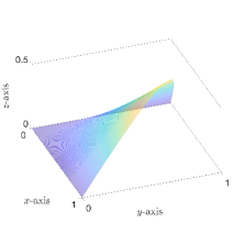
Figure 4: We demonstrate our algorithms on the quadratic triangle $\mathcal{T}$ displayed on the left, which is defined by Eq. 80–Eq. 81 with parameters $a=0.6$, $b=0.7$, and $c=0.5$. For 4D integrals, we integrate over the two quadratic triangles $\mathcal{T}$ and $\mathcal{T}^{\prime}=\mathcal{T}+5\times 10^{-2}(1,1,0)$ shown on the right.

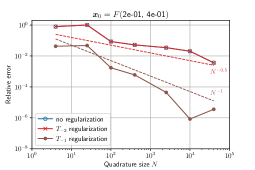
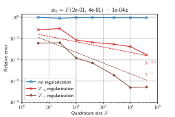
Figure 5: When the singularity is exactly on the triangle, cancellation with the normal leads to a weakly singular kernel. Regularization is not needed to obtain convergence at a rate $\mathcal{O}(N^{-0.5})$, while $T_{-1}$ regularization accelerates the convergence to linear (left). The nearly singular case is harder—the integrand is numerically strongly singular and regularization is needed to converge (right).

Singluar/near-singular integrals over two triangles

We first compute 4D singular integrals of the form of Eq. 71 by integrating twice over the triangle $\mathcal{T}$ defined by Eq. 80–Eq. 81. We combine our method for the $\boldsymbol{x}$-integral with Gauss quadrature for the $\boldsymbol{y}$-integral, and report the results in Fig. 6 (left). The “exact” value is computed with the method of Sauter and Schwab to 8-digit accuracy [27, Chap. 5]. We observe convergence at a rate $\mathcal{O}(M^{-0.5})$ for $T_{-1}$ regularization, where $M$ is the total number of points in 4D. This is consistent with our previous work [17]. To understand this convergence rate, we note that quadrature for the $\boldsymbol{x}$-integral converges at a rate $\mathcal{O}(N^{-1})$ using $T_{-1}$ regularization, while quadrature for the $\boldsymbol{y}$-integral converges at a rate at least $\mathcal{O}(N^{-1})$ since the solid angle $\Omega(\boldsymbol{y})$ is as smooth as the regularized $\boldsymbol{x}$-integrand (they are both of bounded variation), as illustrated in Fig. 7 (left)—the 4D convergence rate is therefore $\mathcal{O}(M^{-0.5})$.

We consider now the case where we integrate over $\boldsymbol{x}\in\mathcal{T}$, where $\mathcal{T}$ is given by Eq. 80–Eq. 81, and $\boldsymbol{y}\in\mathcal{T}^{\prime}=\mathcal{T}+5\times 10^{-2}(1,1,0)$; see Fig. 4 (right). We report the results in Fig. 6 (right). The “exact” value is computed in Mathematica to $6$-digit accuracy. For this example, the method of Sauter and Schwab fails to provide accurate results as it simply utilizes 4D Gauss quadrature, which corresponds to the case with no regularization. (Their method is tailored to the cases where the triangles are identical, or share an edge or a vertex.) Our method converges slightly faster than in the singular case. We emphasize that the solid angle $\Omega(\boldsymbol{y})=\Omega_{-2}(\boldsymbol{y})+\Omega_{-1}(\boldsymbol{y})$ may have sharp variations since $\Omega_{-2}(\boldsymbol{y})$ quickly varies between values around $2\pi$ and $0$ when $\boldsymbol{y}\in\mathcal{T}^{\prime}$ lies below the interior or the exterior of $\mathcal{T}$, as seen in Fig. 7 (right)—however, it is still at least as smooth as the regularized $\boldsymbol{x}$-integrand, so it does not affect the 4D convergence rate.

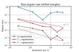
Figure 6: Combining the method described in this paper with Gauss quadrature on triangles yields a method for computing 4D singular integrals of the form of Eq. 71. The method converges at a speed $\mathcal{O}(M^{-0.5})$ with the total 4D number of points $M=N^{2}$ when using $T_{-1}$-regularization.

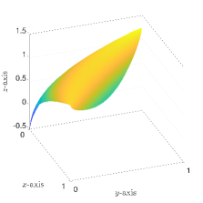
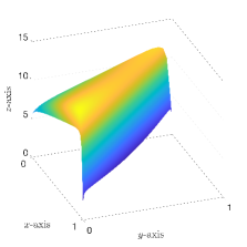
Figure 7: Solid angle function $\Omega(\boldsymbol{y})$ for identical (left) and shifted triangles (right). Despite the sharp variations near the edges, the solid angle function $\Omega(\boldsymbol{y})$ is of bounded variation.

Singluar/near-singular integrals over two triangles (spherical mesh)

We consider a mesh of 84 quadratic triangles, which we generated with Gmsh [8]. (This corresponds to the coarser mesh we will use in Section 4.2 for boundary element computations.) We compute 4D singular integrals of the form of Eq. 71 in three different scenarios: identical triangles, triangles sharing an edge, and triangles sharing a vertex. For each scenario, the reference value is computed to $8$-digit accuracy with the method of Sauter and Schwab. We report the results in Fig. 8.

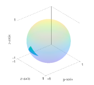
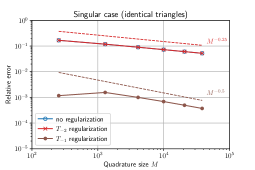
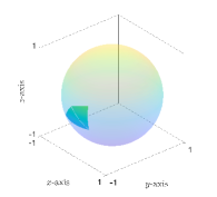
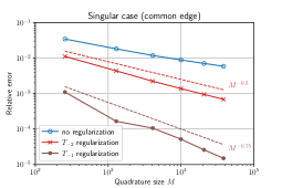
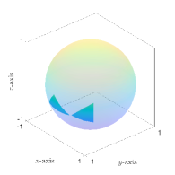
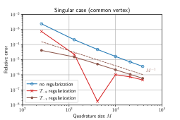
Figure 8: As in the previous experiment, our method converges at a speed $\mathcal{O}(M^{-0.5})$ with the total 4D number of points $M=N^{2}$ when using $T_{-1}$-regularization for identical triangles. For triangles sharing an edge or a vertex, the singularity is somewhat weaker and we observe superconvergence.

4.2 Boundary element computations

We integrate our method into a boundary element code and solve several scattering problems in 3D to illustrate the advantage of using curved elements.

Scattering by a sphere

We consider the sound-soft scattering of a plane wave $u^{i}(r,\theta)=e^{ikr\cos\theta}$ by the unit sphere. We utilize the integral equation Eq. 2 with $\eta=k/2$ and discretize it with a boundary element method with quadratic basis functions ($p=2)$ and quadratic triangles ($q=2$), as described in Section 3.4. We take $k=2\pi$, solve Eq. 2 for $\varphi^{s}$, and evaluate the far-field pattern

(83) $$u_{\infty}(\boldsymbol{\theta})=\frac{1}{4\pi}\int_{\partial D}e^{-ik\boldsymbol{\theta}\cdot\boldsymbol{y}}\varphi^{s}(\boldsymbol{y})dS(\boldsymbol{y}),\quad\boldsymbol{\theta}\in\mathbb{S}^{2},$$

for an increasing number of triangles; see Table 3. For the sphere, the exact pattern is [5, eq. 3.32]

(84) $$u_{\infty}(\theta)=\frac{i}{k}\sum_{n=0}^{\infty}(2n+1)\frac{j_{n}(k)}{h_{n}^{(1)}(k)}P_{n}(\cos\theta),\quad\theta\in[0,2\pi],$$

with Legendre polynomials $P_{n}$, and spherical Bessel and Hankel functions $j_{n}$ and $h_{n}^{(1)}$. We plot the relative error in the far-field pattern in Fig. 9 (left). We observe quartic superconvergence as the mesh size $h\to 0$; cubic convergence was expected. We also display the convergence curve for linear basis functions ($p=1$) and planar triangles ($q=1$).

Table 3: The triangular meshes of the unit sphere, generated by Gmsh [8], comprise up to a million triangles. For linear basis functions ($p=1$), the degrees of freedom (DoFs) are the function values at the vertices. For quadratic basis functions ($p=2$), the DoFs also consist in the function values at the center of the edges.

		DoFs
Mesh size	Triangles	$p=1$	$p=2$
$1.09\times 10^{+0}$	84	44	170
$4.48\text{\times}{10}^{-01}$	324	164	650
$2.57\text{\times}{10}^{-01}$	1,136	570	2,274
$1.35\text{\times}{10}^{-01}$	4,232	2,118	8,466
$7.45\text{\times}{10}^{-02}$	16,310	8,157	32,622
$3.43\text{\times}{10}^{-02}$	65,394	32,699	–
$1.80\text{\times}{10}^{-02}$	258,520	129,262	–
$8.99\text{\times}{10}^{-03}$	1,097,434	548,719	–

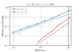
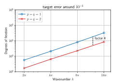
Figure 9: The relative error in the far-field pattern, on the left, decreases like $h^{2}$ for linear basis functions and planar triangles $(p=q=1)$, while it decreases like $h^{4}$ for quadratic basis functions and triangles ($p=q=2$). This is a significant speed-up. A consequence of this, on the right, is that to reach a given target error of around $10^{-3}$ for a given wavenumber $k$, a method with quadratic elements needs four times fewer degrees of freedom.

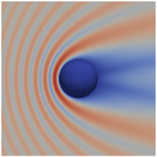
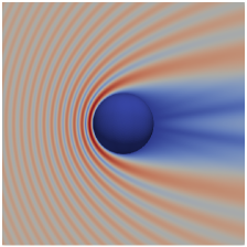
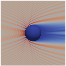
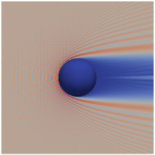
Figure 10: The incident plane wave $u^{i}(r,\theta)=e^{ikr\cos\theta}$ is scattered by the unit sphere. We plot the amplitude of the total field $u^{i}+u^{s}$ for $k=2\pi$ (top left), $k=4\pi$ (top right), $k=8\pi$ (bottom left), and $k=16\pi$ (bottom right). The solution is computed to about six digits of accuracy with a boundary element method with quadratic triangles.

We now take $k\in\{2\pi,4\pi,8\pi,16\pi\}$, solve Eq. 2 for $\varphi^{s}$, and seek the number of degrees of freedom needed to reach a relative error on the far-field pattern around $10^{-3}$ for each $k$. We report the results in Fig. 9 (right). We observe that using quadratic basis functions and triangles reduces the number of degrees of freedom by a factor of about four, while also decreasing computer time by a similar factor at high frequency, as seen in Table 4. All solutions are shown in Fig. 10.

Table 4: To solve the combined boundary integral Eq. 2, one has to assemble the boundary element matrices and then solve the resulting linear system—the dominant cost of the inversion is the computation of the hierarchical $LU$ factors, as discussed in the last paragraph of this section. We display below the computer time, in seconds, to obtain the target error of Fig. 9 (right). We observe that using quadratic elements ($p=q=2$) decreases the total computer time by a factor up to $4.6$ at high frequency.

	$p=q=1$		$p=q=2$
$k$	Assembling matrices	Computing $LU$	Assembling matrices	Computing $LU$
$2\pi$	$1.09\mathrm{e}$$-$$1$	$6.26\mathrm{e}$$-$$2$	$7.55\mathrm{e}$$+$$0$	$4.29\mathrm{e}$$-$$3$
$4\pi$	$1.48\mathrm{e}$$+$$0$	$6.54\mathrm{e}$$+$$0$	$7.39\mathrm{e}$$+$$0$	$1.02\mathrm{e}$$-$$1$
$8\pi$	$8.09\mathrm{e}$$+$$0$	$7.30\mathrm{e}$$+$$1$	$2.59\mathrm{e}$$+$$1$	$1.17\mathrm{e}$$+$$1$
$16\pi$	$8.55\mathrm{e}$$+$$1$	$1.96\mathrm{e}$$+$$3$	$1.40\mathrm{e}$$+$$2$	$3.02\mathrm{e}$$+$$2$

Scattering by half-spheres

We now illustrate the robustness of our method by considering the scattering of a plane wave by two half-spheres of radius one centered at $(0,0,\pm\delta)$ for $\delta=0.5$, $\delta=0.2$, $\delta=0.1$, and $\delta=0$; see Fig. 11. Meshes were created using Gmsh, and the accuracy of the solutions was assessed by comparing them to the numerical solutions presented in [17]. The solutions are correct to about six digits of accuracy.

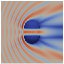
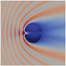
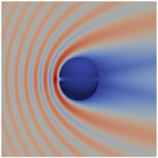
Figure 11: The incident plane wave $u^{i}(r,\theta)=e^{ikr\cos\theta}$ is scattered by two half-spheres of radius one centered at $(0,0,\pm\delta)$. We plot the amplitude of the total field $u^{i}+u^{s}$ for $k=2\pi$ and $\delta=0.5$ (top left), $\delta=0.2$ (top right), $\delta=0.1$ (bottom left), and $\delta=0$ (bottom right). This is a challenging configuration as assembling the boundary element matrices requires to computation of many near-singular integrals.

We conclude this section with a few comments on implementation. We have added our method for computing singular integrals to the C++ castor library of École Polytechnique. The castor library provides tools to create and manipulate matrices à la MATLAB, and uses an optimized BLAS library for fast linear algebra computations. The finest mesh ($h\approx 8.99\times 10^{-3}$) yields dense matrices of size $10^{6}\times 10^{6}$—we employed hierarchical matrices for compression, and, to solve the resulting linear systems, GMRES [25] preconditioned with a hierarchical $LU$ factorization at a lower precision [2]. In this setup, the dominant cost is the computation of the $LU$ factors—GMRES typically converges to a relative residual below $10^{-10}$ in a few iterations. The computations were carried out on an Intel Xeon Gold 6154 processor (3.00 GHz, 36 cores) with 512 GB of RAM.

5 Discussion

We have presented in this paper a novel method for computing strongly singular and near-singular integrals based on singularity subtraction and the continuation approach. This method allows us to solve the Helmholtz exterior Dirichlet problem with a combined boundary integral equation and curved elements. We have demonstrated the accuracy and robustness of our algorithms with several experiments in 3D and have shown numerical evidence that using curved elements is advantageous—it reduces memory usage and computer time by a factor up to four.

We aim to explore various strategies to improve the efficiency of curved boundary element methods. One strategy we are considering is using the continuation approach on curved patches directly. Currently, our method involves projecting the patches onto a reference flat domain, which leads to complex formulas and the computation of 2D integrals. However, if we could use the continuation approach directly, we would only need to deal with smooth 1D integrals on the patches’ boundaries, significantly reducing computational time and making curved boundary element methods even more attractive. This could be based on the generalized Stokes theorem for differential forms, similarly to [32]. Lastly, one of the drawbacks of our method is the lack of rigorous justification of the convergence speeds. To address this, we plan to prove rigorous error bounds, starting with the weakly-singular case. These bounds will be based on convergence results for Gauss-Legendre quadrature rules for functions of limited regularity [31].

Appendix A Elasticity potentials

Elastodynamics requires the computation of singular integrals of the form of

(86) $$\widetilde{I}(\boldsymbol{x}_{0})=\int_{\mathcal{T}}\frac{(\boldsymbol{x}-\boldsymbol{x}_{0})\cdot\boldsymbol{e}}{|\boldsymbol{x}-\boldsymbol{x}_{0}|^{3}}\varphi(F^{-1}(\boldsymbol{x}))dS(\boldsymbol{x}),$$

for some arbitrary unit vector $\boldsymbol{e}$; see, e.g., [3]. Following steps 1–2 of Section 3 leads to

(87) $$\widetilde{I}(\boldsymbol{x}_{0})=\int_{\widehat{T}}\frac{(F(\boldsymbol{\hat{x}})-F(\boldsymbol{\hat{x}}_{0})-h\boldsymbol{\hat{n}}_{0}/|\boldsymbol{\hat{n}}_{0}|)\cdot|\boldsymbol{\hat{n}}(\boldsymbol{\hat{x}})|\boldsymbol{e}}{|F(\boldsymbol{\hat{x}})-\boldsymbol{x}_{0}|^{3}}\varphi(\boldsymbol{\hat{x}})dS(\boldsymbol{\hat{x}}).$$

We compute the asymptotic term $\widetilde{T}_{-2}$,

(88) $$\widetilde{T}_{-2}(\boldsymbol{\hat{x}},h)=\frac{\left[J_{0}(\boldsymbol{\hat{x}}-\boldsymbol{\hat{x}}_{0})-h\boldsymbol{\hat{n}}_{0}/|\boldsymbol{\hat{n}}_{0}|\right]\cdot|\boldsymbol{\hat{n}}_{0}|\boldsymbol{e}}{\left[|J_{0}(\boldsymbol{\hat{x}}-\boldsymbol{\hat{x}}_{0})|^{2}+h^{2}\right]^{\frac{3}{2}}}\varphi_{0}.$$

For the new term in Eq. 88, we apply Theorem 3.1 with $\ell=0$. This yields

(89) $$\widetilde{I}_{-2}(\boldsymbol{x}_{0})=\, \varphi_{0}\sum_{j=1}^{3}\hat{s}_{j}\int_{\partial\widehat{T}_{j}-\boldsymbol{\hat{x}}_{0}}\left(J_{0}\boldsymbol{\hat{x}}\cdot|\boldsymbol{\hat{n}}_{0}|\boldsymbol{e}\right)\widetilde{g}_{-2}(\boldsymbol{\hat{x}},h)ds(\boldsymbol{\hat{x}})$$

$$-\mathrm{sign}(h)\varphi_{0}\left(\boldsymbol{\hat{n}}_{0}\cdot\boldsymbol{e}\right)\sum_{j=1}^{3}\hat{s}_{j}\int_{\partial\widehat{T}_{j}-\boldsymbol{\hat{x}}_{0}}\frac{\sqrt{|J_{0}\boldsymbol{\hat{x}}|^{2}+h^{2}}-|h|}{|J_{0}\boldsymbol{\hat{x}}|^{2}\sqrt{|J_{0}\boldsymbol{\hat{x}}|^{2}+h^{2}}}ds(\boldsymbol{\hat{x}}),$$

where the one-dimensional integrand $\widetilde{g}_{-2}$ is defined by

(90) $$\widetilde{g}_{-2}(\boldsymbol{\hat{x}},h)=-\frac{1}{|J_{0}\boldsymbol{\hat{x}}|^{2}\sqrt{|J_{0}\boldsymbol{\hat{x}}|^{2}+h^{2}}}+\frac{\mathrm{arcsinh}\left(\frac{|J_{0}\boldsymbol{\hat{x}}|}{|h|}\right)}{|J_{0}\boldsymbol{\hat{x}}|^{3}}.$$

When $h=0$, the first term in Eq. 90 integrates to $0$ (it is the residue of Theorem 3.1), while the second term may be replaced by $\log|\boldsymbol{\hat{x}}|/|J_{0}\boldsymbol{\hat{x}}|^{3}$ (it is the Cauchy principal value).

References

- [1] M. H. Aliabadi, W. S. Hall, and T. Phemister, Taylor expansions for singular kernels in the boundary element method, Internat. J. Numer. Methods Engrg., 21 (1985), pp. 221–2236.
- [2] M. Bebendorf, Hierarchical LU decomposition-based preconditioners for BEM, Computing, 74 (2005), pp. 225–247.
- [3] S. Chaillat, M. Darbas, and F. Le Louër, Fast iterative boundary element methods for high-frequency scattering problems in D elastodynamics, J. Comput. Phys., 341 (2017), pp. 429–446.
- [4] D. Colton and R. Kress, Integral Equation Methods in Scattering Theory, SIAM, Philadelphia, 1983.
- [5] D. Colton and R. Kress, Inverse Acoustic and Electromagnetic Scattering Theory, Springer, New York, 3rd ed., 2013.
- [6] M. G. Duffy, Quadrature over a pyramid or cube of integrands with a singularity at a vertex, SIAM J. Numer. Anal., 19 (1982), pp. 1260–1262.
- [7] L. Faria, Pérez-Aranciabia, and M. Bonnet, General-purpose kernel regularization of boundary integral equations via density interpolation, Comput. Methods Appl. Mech. Engrg., 378 (2021), p. 113703.
- [8] C. Geuzaine and J.-F. Remacle, Gmsh: a three-dimensional finite element mesh generator with built-in pre- and post-processing facilities, Internat. J. Numer. Methods Engrg., 79 (2009), pp. 1309–1331.
- [9] M. Guiggiani and A. Gigante, A general algorithm for multidimensional Cauchy principal value integrals in the boundary element method, ASME J. Appl. Mech., 57 (1990), pp. 906–915.
- [10] M. Guiggiani, G. Krishnasamy, T. J. Rudolphi, and F. J. Rizzo, A general algorithm for the numerical solution of hypersingular boundary integral equations, ASME J. Appl. Mech., 59 (1992), pp. 603–614.
- [11] N. Hale and L. N. Trefethen, New quadrature formulas from conformal maps, SIAM J. Numer. Anal., 46 (2008), pp. 930–948.
- [12] W. S. Hall and T. T. Hibbs, Subtraction, expansion and regularising transformation methods for singular kernel integrations in elastostatics, Math. Comput. Model., 15 (1991), pp. 313–323.
- [13] B. Johnston, P. R. Johnston, and D. Elliott, A new method for the numerical evaluation of nearly singular integrals on triangular elements in the D boundary element method, J. Comput. Appl. Math., 245 (2013), pp. 148–161.
- [14] A. Klöckner, A. Barnett, L. Greengard, and M. O’Neil, Quadrature by expansion: A new method for the evaluation of layer potentials, J. Comput. Phys., 252 (2013), pp. 332–349.
- [15] M. Lenoir and N. Salles, Evaluation of D singular and nearly singular integrals in Galerkin BEM for thin layers, SIAM J. Sci. Comput., 34 (2012), pp. A3057–A3078.
- [16] F. M. Lether, Computation of double integrals over a triangle, J. Comput. Appl. Math., 2 (1976), pp. 219–224.
- [17] H. Montanelli, M. Aussal, and H. Haddar, Computing weakly singular and near-singular integrals over curved boundary elements, SIAM J. Sci. Comput., 44 (2022), pp. A3728–A3753.
- [18] J. C. Nédélec, Curved finite element methods for the solution of singular integral equations on surfaces in , Comput. Methods Appl. Mech. Engrg., 8 (1976), pp. 61–80.
- [19] C. Pérez-Arancibia, C. Turc, and L. Faria, Planewave density interpolation methods for D Helmholtz boundary integral equations, SIAM J. Sci. Comput., 41 (2019), pp. A2088–A2116.
- [20] X. Qin, J. Zhang, X. Guizhong, Z. Fenglin, and L. Guanyao, A general algorithm for the numerical evaluation of nearly singular integrals on D boundary element, J. Comput. Appl. Math., 235 (2011), pp. 4174–4186.
- [21] M. T. H. Reid, K. White, J, and S. G. Johnson, Generalized Taylor–Duffy method for efficient evaluation of Galerkin integrals in boundary-element method computations, IEEE Trans. Antennas and Propagation, 63 (2015), pp. 195–209.
- [22] D. Rosen and D. E. Cormack, Singular and near singular integrals in the BEM: A global approach, SIAM J. Appl. Math., 53 (1993), pp. 340–357.
- [23] D. Rosen and D. E. Cormack, The continuation approach: A general framework for the analysis and evaluation of singular and near-singular integrals, SIAM J. Appl. Math., 55 (1995), pp. 723–762.
- [24] E. Ruiz-Gironés, J. Sarrate, and X. Roca, Measuring and improving the geometric accuracy of piece-wise polynomial boundary meshes, J. Comput. Phys., 443 (2021), p. 110500.
- [25] Y. Saad and M. H. Schultz, GMRES: A generalized minimal residual algorithm for solving nonsymmetric linear systems, SIAM J. Sci. Statist. Comput., 7 (1986), pp. 856–869.
- [26] N. Salles, Calcul des singularités dans les méthodes d’équations intégrales variationnelles, PhD thesis, Université Paris-Sud, 2013.
- [27] S. Sauter and C. Schwab, Boundary Element Methods, Springer, Berlin, 2011.
- [28] E. A. Spence, I. V. Kamotski, and V. P. Smyshlyaev, Coercivity of combined boundary integral equations in high-frequency scattering, Comm. Pure Appl. Math., 68 (2015).
- [29] A. Van Oosterom and J. Strackee, The solid angle of a plane triangle, IEEE Trans. Biomed. Eng., BME-30 (1983), pp. 125–126.
- [30] S. Vijayakumar and D. E. Cormack, A new concept in near-singular integral evaluation: The continuation approach, SIAM J. Appl. Math., 49 (1989), pp. 1285–1295.
- [31] S. Xiang and F. Bornemann, On the convergence rates of Gauss and Clenshaw–Curtis quadrature for functions of limited regularity, SIAM. J. Numer. Anal., 50 (2012).
- [32] H. Zhu and S. Veerapaneni, High-order close evluation of Laplace layer potentials: A differential geoemtric approach, SIAM J. Sci. Comput., 44 (2022), pp. A1381–A1404.