Exploring the unique properties of gravastars exhibiting string clouds and quintessence
Abstract
Gravastars, theoretical alternatives to black holes, have captured the interest of scientists in astrophysics due to their unique properties. This paper aims to further investigate the exact solution of a novel gravastar model based on the Mazur-Mottola (2004) method within the framework of general relativity, specifically by incorporating the cloud of strings and quintessence. By analyzing the gravitational field and energy density of gravastars, valuable insights into the nature of compact objects in the universe can be gained. Understanding the stability of gravastars is also crucial for our comprehension of black holes and alternative compact objects. For this purpose, we presents the Einstein field equations with the modified matter source and calculate the exact solutions for the inner and intermediate regions of gravastars. The exterior region is considered as a black hole surrounded by the cloud of strings and quintessence, and the spacetimes are matched using the Darmoise-Israel formalism. The stability of gravastars is explored through linearized radial perturbation, and the proper length, energy content, and entropy of the shell are calculated. The paper concludes with a summary of the findings and their implications in the field of astrophysics and cosmology.
Keywords: Gravastar; cloud of strings; quintessence field; stability analysis.
I Introduction
Astrophysical objects known as black holes, which are the mathematical solutions to the Einstein equations, are widely acknowledged. Two significant observations about black holes in our universe were recently reported. The first is the discovery of gravitational waves coming from black hole binaries 1m ,2m , and the second is the discovery of photographic proof of black holes at the centers of our galaxy’s M87 and Sgr A* 3m ,4m . But distant observers should be able to observe phenomena that happen outside the event horizon or even before they form. As a result, it is still unclear whether an astrophysical object has an event horizon. Several authors have suggested that the gravitational collapse of a massive star could make the densest celestial objects other than black holes. To address this idea, Mazur and Mottola introduced a new theory of collapsing stellar objects known as gravitational vacuum stars, or “gravastars”, which incorporates the expanded concept of Bose-Einstein condensation in the gravitational system. Gravastar has been proposed as a black hole substitute that also takes into account quantum effects 5m ,6m . The gravastar model is believed to offer a solution to issues associated with traditional black holes, while also meeting all theoretical requirements for a stable endpoint of stellar evolution. This theory suggests that quantum vacuum fluctuations play a significant role in collapse dynamics, leading to a phase transition that results in a repulsive de Sitter core that balances the collapsing body and prevents the formation of a horizon (and singularity) near the bound of . However, this phenomenon occurs very close to the limit, making it challenging for an outsider to differentiate between a gravastar and a true black hole.
Gravastars exhibit a distinctive structure characterized by three distinct zones. The internal region () consists of an isotropic de Sitter core governed by the equation of state (EoS) . The external zone () corresponds to the vacuum and is described by the Schwarzschild geometry, with an EoS of . Separating these internal and external regions is a thin shell () of stiff matter having EoS , where and depict the internal and external radii of gravastar. After the proposal of Mazur and Mottola, enormous discussion has been done on gravastar. Visser and Wiltshire 3 analyzed the stable structure of gravastars and examined that distinct EoSs yield the dynamically stable configuration of gravastars. Carter 4 presented novel exact gravastar solutions and observed the impact of EoS on different zones of gravastar geometry. Bilić et al. 5 obtained the gravastars solutions by considering the Born-Infeld phantom instead of de Sitter spacetime and observed that at the center of stars, their findings can manifest the dark compact configurations.
The role of energy limits within the gravastar shell and its stability were investigated by Horvat and Ilijic 6 using radial perturbations and the sound speed on the shell. Various researchers 7 -12 have explored the internal structure of the gravastar using different equations of state. Lobo and Arellano 13 built several gravastar models that incorporated nonlinear electrodynamics and discussed specific characteristics of their models. Horvat et al. 14 extended the concept of gravastar by introducing an electric field and examined the stability of both the internal and external regions. In a similar vein, Turimov et al. 15 studied the effects of a magnetic field on the gravastar geometry and obtained precise solutions for a slowly rotating gravastar. The stability of thin-shell gravastars developed from inner nonsingular de Sitter manifold and outer charged noncommutative black hole solution by using Visser’s cut and paste approach is discussed in 15q .
In the field of cosmology, researchers have developed modified gravitational theories as alternatives to general relativity (GR) in order to explain the causes behind the expansion of the universe. These theories introduce different approaches, such as gravity 16 , gravity 17 , and theory 18 , where represents the curvature invariant, represents the trace of the energy-momentum tensor (EMT), and represents the Gauss-Bonnet invariant. The study of gravastar geometries has motivated researchers to investigate the effects of these extended gravitational theories on different types of gravastars. In the context of gravity, Das et al. 19 explored the concept of gravastar geometry and analyzed its characteristics using graphical methods for various equations of state (EoSs). Shamir and Ahmad 20 derived non-singular solutions for gravastars and obtained mathematical expressions for various physical parameters within the framework of theory. Sharif and Waseem 21 investigated the influence of the Kuchowicz metric potential on the structure of gravastars in theory. Sharif and Naz 25 ,26 studied important aspects of gravastars in the absence and presence of an electric field within the framework of gravity. Usmani et al. 27 utilized these Killing vectors to investigate various aspects of gravastars with electric charge, obtaining solutions that corresponded to different eras of gravastar evolution. They specifically focused on the influence of conformal vectors on the gravastar structure. Sharif and Waseem 28 examined the impact of charge on the gravastar’s structure within the framework of theory, taking into account the conformal Killing vectors. Bhar and Rej 29 proposed a charged gravastar model that incorporated conformal motion within the framework of theory. They explored the consequences of this motion on the properties of the charged gravastar. Sharif and his collaborators 30 ,31 investigated analytic solutions for both charged and uncharged gravastar models using conformal Killing vectors in the context of theory.
The presence of dark energy in black holes aligns with the standard model of cosmology, which indicates its dominance in the universe 38q ,39q . This interaction between dark energy and black holes, similar to the cosmological constant or vacuum energy, can have significant implications 41q . Astronomical observations have shown that the universe is expanding at an accelerating rate, implying the existence of negative pressure, which can be explained by quintessence dark energy 42q -45q . Theoretical advancements propose that one-dimensional strings, rather than point-like particles, are the fundamental units of nature. Exploring Einstein’s equations with string clouds is crucial, as relativistic strings can be used to construct appropriate models 54q . The concept of a cloud of strings as the source of the gravitational field was initially introduced by Lately, who discovered an exact solution for a Schwarzschild black hole surrounded by strings 54q ,55q . The effects of both quintessence and cloud of strings on the black hole thermodynamics are explored in 60q .
The concept of gravastars, which are theoretical alternatives to black holes, has captured the interest of scientists and researchers in the field of astrophysics. However, there is still much to be explored and understood about these intriguing objects. The motivation behind this paper lies in the desire to further investigate the exact solution of gravastars within the framework of general relativity, specifically by incorporating the cloud of strings and quintessence. The paper is organized as follows: In section-II, we present the Einstein filed equations with the presence of modified matter source as cloud of strings and quintessence. In section-III, we calculate the exact solutions of inner, outer regions of gravastars. Then, we consider exterior region as a black hole surrounded by cloud of strings and quintessence. Then, we math these spacetimes through well-known Darmoise-Israel formalism as present in In section-IV. Section-V is denoted to explore the stability of gravastars using linearized radial perturbation and also calculate the proper length, energy content, entropy of the shell. Last section devoted to present the concluding remarks.
II Assessing the Impacts of cloud of strings and quintessence on Einstein’s Field Equations
The focus of this section is on the 4-dimensional spacetime that is both spherically symmetric and static, and it is bounded by a spherical surface. Using the Schwarzschild coordinates, the respective metric is presented as follows
| (1) |
here the gravitational functions of temporal and radial coordinates are denoted by and , respectively. By using the modified form of matter, the respective Einstein field equations for the metric (1) become
| (2) |
where
| (3) |
here represents the matter due to cloud of string and depicts the matter influenced by quintessence fields. Consequently, in the background of strings of clouds, the respective Lagrangian density can be written as 122
| (4) |
where the tension of the string and bi-vector is denoted by a constant . In this regards, we obtain the following relation
| (5) |
here relation for the parameterization of the world sheet is referred as and Levi-Civita tensor is represented by . By using induced metric, it can be described for the string as follows 122
| (6) |
Consequently, the some important identities is obtained from given as 122 , 123
| (7) |
where the determinant of is denoted with h.
Further, by varying the Lagrangian density with respect to the metric tensor , we get 123
| (8) |
where denotes the density of the string cloud. We obtain the following expression by considering the identities mentioned in Eq.(7). In the background of string clouds, the respective components of stress-energy tensor become 124 :
| (9) |
where the parameter denotes the cloud of strings. Also, we obtain the following relation for quintessence matter distribution as follows 125
| (10) |
The stress-energy-momentum tensor components that are physically viable under the influence of the quintessence field () are specified by , which denotes the potential term of the quintessence field. 122 , 126
| (11) |
where and denote the quintessence field parameter and quintessence density, respectively, and are used to characterize the system’s internal makeup in the presence of the matter source . To analyze the physical composition of spacetime, we examine the energy density of an isotropic matter distribution that covers the area. Here, the radial pressure is represented by and the energy density is depicted with . Further, the respective components of stress-energy tensor become
| (12) |
Consequently, we get the modified form of field equations (2) in the presence of cloud of strings and quintessence field given as
| (13) | |||
| (14) | |||
| (15) |
where the derivative with respect to radial component is denoted by primes. Now, by solving the above field equations for , , and , we get the following expressions for the corresponding quantities:
| (16) | |||||
| (17) | |||||
| (18) |
Now, for the GR gravity the energy conservation equation under the current scenario can be provided as
| (19) |
From the equation mentioned above, it becomes apparent that for a gravitating system to be in a state of equilibrium, the force of gravity must be counter balanced by an equal pressure gradient known as the hydro-static force.
Further, we are interested to develop gravastar structure in the background of cloud of strings and quintessence by using the exact field equations with modified matter source. Overall, the gravastar configuration with cloud of strings and quintessence is a fascinating model that may shed light on the nature of dark energy and the origins of the universe. Gravastar is a hypothetical model that is formed from the collapse of matter in the presence of a negative pressure source which can be better explained by quintessence field. Quintessence is a form of dark energy that is believed to be responsible for the acceleration of the universe’s expansion. In this model, the gravastar consists of a thin-shell of negative pressure, surrounded by a thick shell of ultra-relativistic cosmic string. The cosmic string is a hypothetical one-dimensional object that is formed from the stretching of space-time due to the presence of a concentrated mass. The configuration of the gravastar is such that the cosmic string provides the necessary self-gravity to support the quintessence shell. The negative pressure of the quintessence further contributes to the self-gravity of the system, creating a stable equilibrium. One interesting property of the gravastar configuration is that it can be allowed for the existence of stable orbits within the object. This is due to the fact that the quintessence shell exerts gravitational pull on nearby masses, while the cosmic string shell provides a repulsive force. The combination of these forces can be leads to the creation of a stable region within the gravastar where orbits can be maintained.
III Gravastar configuration with string and quintessence
In this section, we develop the gravastar structure by using the field equation in the framework of modified matter source. For this purpose, we devlop the gravastar by understanding its geometrical structure which can be partitioned into three different regions. The behavior of matter contents of these regions can be chracterized through specific type of EoS. Such geometrical structure is partitioned into interior (), intermediate or thin-shell () and exterior region (). Here, and denote the radius of inner and outer regions. Also, the thickness of the intermediate region is referred as . The specific EoS for these regions are expressed as
-
•
for inner region;
-
•
for intermediate region;
-
•
for outer region.
In the following subsections, we discuss in detail the solution of these regions by using the respective EoS.
III.1 Interior region of the gravastar with string and quintessence
The relationship between the metric potentials and the physical parameters like and from Eq. (16) and Eq. (17) by using the interior area as stated in Mazur, Mottola’s work is provided below:
| (20) |
the parameterized version of this EoS is known as the dark energy EoS with . This negative pressure acts radially outwards from the center of the spherically symmetric gravitating system, counteracting the inward gravitational attraction of the shell. It can be shown, by using Eq. (20) in Eq. (19) as
| (21) |
where represents the critical density of the gravastar. Now, by the help of Eq. (20) within the scope of the Eqs. (16) and (17), we have following relation
| (22) |
Now, by solving the Eq. (22), we have the following connection between gravitational metric components:
| (23) |
here represents the constant of integration. Now, by plugging the Eqs. (21) and (23) in Eq. (16), we have following differential equation:
| (24) |
It is noticed that, the above equation is depending on one gravitational metric components, i.e., , and quintessence field . Now, we can solve the above differential equation for the specific value of , which should posing quintessence matter. In this regard, we shall choose, (quintessence matter), and get the following expression for as:
| (25) |
where and are constants of integration. For the purpose of the regular solution at the center, we must impose the condition, i.e., . Finally, we have the following simplified relation for metric component written as
| (26) |
Now, by using the Eq. (26) in Eq. (23), we have the following metric component:
| (27) |
III.2 Intermediate region
Herein, we calculate the exact solution for intermediate region with physical parameters in the framework of EoS, which is defined as
| (28) |
Now, by plugging the Eqs. (16) and (17) in Eq. (28), we have the following relation
| (29) | |||||
The intermediate shell is assumed to be created by an ultra-relativistic fluid with a non-vacuum background and an EoS . In the non-vacuum zone, it is difficult to determine the solution to the complicated set of field equations. To avoid this inquiry, we will make some approximations and discover an analytical answer, namely, . We use the embedded technique to find the precise answer, i.e. the product terms of metric functions and derivative of metric component become vanish as . In this regard, we get a modified version of field equations in the simplified form as:
| (30) |
On solving the above equation, one can get the following expression for metric component:
| (31) |
with as integrating constant. For the metric component, we make a use of Eq. (19) and get the following relation of the metric components:
| (32) |
Now, again we are adopting the embedded procedure as mentioned above and get the following final differential equation:
| (33) |
By plugging the Eq. (31) in Eq. (33), one can get the following expression for metric component:
| (34) |
where is an integrating constant. By using these metric function in the energy conservation equation for stiff matter distributions, we get
| (35) |
with integrating constant .
III.3 The Exterior Region
A black hole with quintessence and cloud of strings would be a very interesting and complex phenomenon. Quintessence is a theoretical form of dark energy that is thought to be responsible for the accelerating expansion of the universe. It is a hypothetical scalar field that permeates all of space and time, and it has the potential to affect the behavior of objects near a black hole. Cloud strings are another hypothetical phenomenon that could potentially exist in the vicinity of a black hole. They are thin, long, and extremely dense configurations of matter that are thought to form in the early universe. These cloud strings could exist in the vicinity of a black hole and modify its properties. Combining these two phenomena, we can imagine a black hole that is surrounded by a cloud of quintessence and cloud strings. This could have a number of interesting effects on the black hole, including altering its mass, spin, and other properties. For example, the presence of the quintessence field could have the effect of slowing down the rate at which matter and energy fall into the black hole. This could in turn reduce the rate at which the black hole grows in mass over time. The presence of the cloud strings could also modify the behavior of particles in the vicinity of the black hole, potentially leading to novel and unexpected phenomena. In the present work, we are interested to observe the affects of both cloud of strings and quintessence on the geometrical structure of gravastars. In this regards, we consider the exact solution of the black hole geometry surrounded by cloud of strings and quintessence as an exterior manifold 60q . The line element of such black hole geometry can be expressed as 60q
| (36) |
where stands for the Kiselev parameter. In the absence of and , the considered black hole geometry reduces to the Schwarzschild black hole.
IV Matching of interior and exterior regions through junction conditions
In order to develop the geometry of gravastar, we match the exact solutions of exterior (+) and interior (-) regions through junction conditions. These geoemtries are matched at the hypersurface by implementing Visser cut and paste approach q1 ; q2 ; q3 . Hence, we cut inner and outer manifolds into the following regions as
| (37) |
during this Darmois-Israel formalism, it is necessary to maintain the radius of shell () must be greater then the radius of event horizon of the considered exterior black hole spacetime. In this approach, the developed structure is free from event horizon as well as the spacetime singularity q1 ; q2 ; q3 . Both, spacetimes are connected at the hypersurface () which is (2+1)-dimensional manifold given as
| (38) |
Hence, we get the unique regular spacetime which can be written as mathematically as . The coordinates of hypersurface and manifolds have the following form , , respectively. Here proper time is represented with . Also, the coordinates of hypersurface and the manifolds are connected through the following coordinate transformation
| (39) |
Consequently, the hypersurface parametric equation can be written as
The thin layer of matter content located at the shell is very important to discuss the dynamics as well as stable configuration of the shell. The surface pressure and the energy density of the matter can be evaluated through the Lanczos equations given as q1 ; q2 ; q3
| (40) |
where and represents the components of extrinsic curvature. The energy-momentum tensor for the perfect fluid can be written as where and denotes the energy density and surface pressure of ideal fluid. Also, the components of extrinsic curvature are written as
| (41) |
where denoted the normal vector which can be given as
| (42) |
here over dot represents the derivative with respect to the proper time. By employing the Lanczos equations, we obtain
| (43) | |||||
| (44) |
The surface pressure and energy density of shell follows the energy conservation constraints as
which leads to
It is noted that the equilibrium position of the shell () leads to vanishing of derivative of shell radius with respect to the proper time, i.e., .. At equilibrium shell radius, shell does not move in the radial direction. Hence, we have
| (45) | |||||
| (46) |
where and are the energy density and pressure at equilibrium position, respectively.
V Some Physical characteristics of Gravastars
This section is devoted to examine the impact of cloud of strings and quintessence field on different physical features of gravastar. In this context, we shall calculate the stability through linearized perturbation. Then, we observe the proper length, shell energy and entropy of the gravastars.
V.1 Stability with Linearized Radial Perturbation
First, we calculate the equation of motion of the shell from Eq. (43) as
| (47) |
where depicts the potential function which can be calculated as
| (48) | |||||
We are interested to perturb the system about equilibrium shell radius to explore the stability of the gravastars. In this regards, we expand potential function around using Taylor series up to 2nd order terms . Hence, we get
| (49) |
By using the conservation equation, we get
Now, we consider the following parameter for the second derivative of the potential function as
It is interesting to mention that and . Hence, we have
| (50) |
consequently, the equation of motion become
| (51) |
Thus, the developed structure become stable if otherwise unstable. Hence, the stability condition of the developed structure can be characterized as
| (52) |
where
where
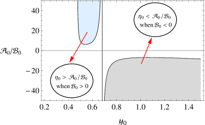
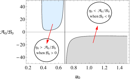

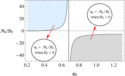
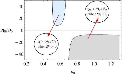
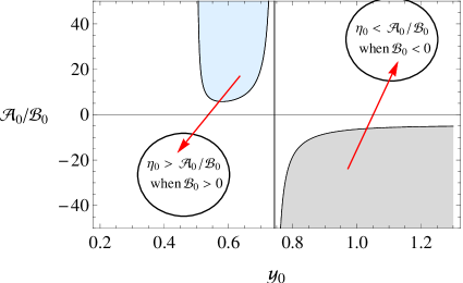
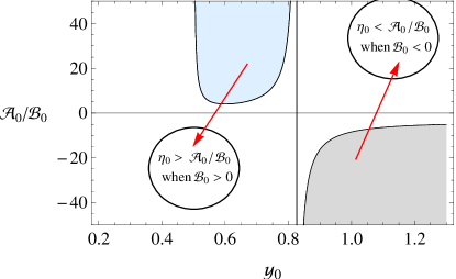
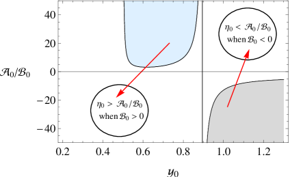
In Figs. (1) and (2), we are interested to explore the stable configuration of the gravastars in the framework of quintessence and cloud of strings. It is very interesting to mention that the stable regions of the gravastars greatly affected by the presence of cloud of strings and quintessence field parameters. It is found that stable regions increases as the cloud of strings parameter increases. This shows that the developed structure is more stable due to the effects of cloud of strings (Figs. (1)). It is found that the stability regions decreases as quintessence field parameter increases as shown in (Figs. (2)). Hence, both quintessence and cloud of strings play a remarkable to maintain the stability of gravatars.
V.2 Proper Length of the Thin Shell
We are interested to discuss the proper length of the shell and the thickness of the shell is represented by . The shell thickness is a very small positive real number such as . The lower and upper boundaries of the shell are and . Mathematically, the proper length of the shell can be evaluated as qm
| (53) |
In order to solve the above complicated integration, we assume that the as
| (54) |
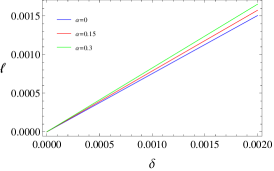
where is a very small positive real constant, therefore, its square and higher powers must be ignored. In this regard, we obtain a relationship between the thickness and the proper length of shell. This relation depends on the shell radius and cloud of strings parameter. The behavior of proper length versus thickness of the shell for different values of cloud of quintessence are shown in the left plot of Fig. (3). Proper length increases as thickness as well as cloud of strings parameter increases.
V.3 Energy content
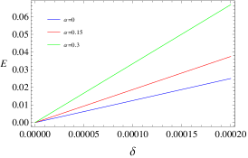
The inner region of gravastar is negative energy zone with non-attractive force and matter obey the EoS . Applying the same technique, such as determining the proper length, the energy distribution in the shell’s region can be evaluated as qm
| (55) |
The final expression of the shell energy is directly related with shell radius, thickness and cloud of strings parameter. Hence, the cloud of strings parameter directly effects the energy of the shell. The graphical analysis of energy content versus thickness of the shell for different values of cloud of quintessence are shown in middle plot of Fig. (3). It increases as thickness as well as cloud of strings parameter increases.
V.4 Entropy
The degree of disorder or disturbance in a geometric structure is related to the entropy measure. To understand the randomness of gravastar geometry, we look at the entropy of thin-shell gravastars. Mazur and Mottola’s idea is used to calculate an equation for the entropy of a thin-shell gravastar as qm
| (56) |
For local temperature, the entropy density is calculated as
| (57) |
where represented as a dimensionless parameter. Here, we take Planck units so that the shell’s entropy becomes qm
| (58) |
It is noted that shell’s entropy is also proportional to . Similarly, we investigate entropy of the shell along thickness of the shell for different values of cloud of strings are shown in right plot of Fig. (3). It is noted that the entropy increases by increasing as well as cloud of strings parameter.

VI Conclusion
The motivation behind the gravastar solution with a modified matter source in the background of a cloud of strings and quintessence is to explore alternative models of gravastars and study their implications in the context of string theory and dark energy. Gravastars are hypothetical objects that have been proposed as an alternative to black holes. They are thought to be made up of exotic matter that can prevent the formation of an event horizon, which is a defining feature of black holes. Instead, gravastars have a surface called a “gravitational vacuum star” that can mimic some of the properties of a black hole without the singularity at its center. In this particular scenario, the background is assumed to be a cloud of strings. String theory is a theoretical framework that attempts to reconcile quantum mechanics and general relativity by describing fundamental particles as tiny, vibrating strings. The cloud of strings provides a unique environment for studying the behavior of gravastars and their interaction with the underlying string structure. Additionally, quintessence is a form of dark energy that is hypothesized to explain the accelerating expansion of the universe. By incorporating quintessence into the gravastar solution, researchers aim to investigate the potential interplay between exotic matter, string theory, and dark energy. Overall, the motivation for studying the gravastar solution with a modified matter source in the background of a cloud of strings and quintessence is to explore novel theoretical frameworks, investigate alternative models of black hole-like objects, and gain a deeper understanding of the fundamental nature of the universe. For this purpose, we developed the Einstein field equation in the framework of modified matter source. Further, we have calculated the gravastar structure and their physical properties as mentioned below:
-
•
Inner region: By applying the EoS to the interior region and analyzing the equations of motion and conservation equation, it has been established that the solution does not have a singularity. Additionally, the energy density and pressure of the system remain constant, which is consistent with the characteristics associated with dark energy.
-
•
Intermediate thin shell: We have considered the EoS that follows the intermediate shell condition and also determined the respective metric potential.
-
•
Outer region: We have used the exact black hole solution surrounded by cloud of strings and quintessence as an outer manifold. Then, we have developed the gravastar structure by considering Darmois-Israel formalism. The detailed outcomes related to stability and physical properties of gravastars are given below:
-
1.
Stability analysis: We are interested to explore the effects of cloud of strings and quintessence on the stability of gravastar structure through linearized perturbation. It is noted that cloud of strings parameter enhances the stable regions of gravastars and stability decreases as decreases as shown in Fig. (1). The quintessence field parameter also effects the stability of the gravastars. The stable region decreases as the quintessence field parameter increases see Fig. (2).
-
2.
Proper length: We have established a connection between the thickness of the shell and its proper length. This connection is influenced by both the radius of the shell and the parameter representing the cloud of strings. The left plot in Fig. (3) illustrates how the proper length changes with varying thickness of the shell for different values of the cloud of quintessence. As both the thickness and the cloud of strings parameter increase, the proper length also increases.
-
3.
Energy: The equation for the energy of the shell is directly dependent on the shell radius, thickness, and the parameter representing the cloud of strings. As a result, the energy of the shell is directly influenced by the cloud of strings parameter. The middle plot in Fig. (3) illustrates how the energy content changes with varying thickness of the shell for different values of the cloud of strings. The energy content increases as both the thickness and the cloud of strings parameter increase.
-
4.
Entropy: The analysis reveals that the entropy of the shell’s region is directly proportional to the thickness of the shell. Likewise, we examine the entropy of the shell as we vary its thickness for different values of the cloud of strings. This investigation is depicted in the right plot of Fig. (3). It is worth noting that the entropy increases as both the thickness and the cloud of strings parameter increase.
-
1.
It is concluded that the gravastar solutions in the presence of cloud of strings and quintessence fields having attractive features. We have developed a singularity free solution which is physically acceptable. It is interesting to mention that the developed exact novel solutions are reduced to the exact Mazur and Mottola model in the absence of cloud of strings and quintessence fields.
Acknowledgement
F. Javed acknowledges the financial support provided through Grant No. YS304023917, which has contributed to his Postdoctoral Fellowship at Zhejiang Normal University.
References
References
- (1) Abbott, B. P. et al. [LIGO Scientific and Virgo], Phys. Rev. Lett. 116, no.6, 061102 (2016).
- (2) Abbott, R. et al. [LIGO Scientific, VIRGO and KAGRA], [arXiv:2111.03606 [gr-qc]].
- (3) Akiyama, K. et al. [Event Horizon Telescope], Astrophys. J. Lett. 875, L1 (2019).
- (4) Akiyama, K. et al. [Event Horizon Telescope], Astrophys. J. Lett. 930, no.2, L12 (2022).
- (5) Mazur, P. O. and Mottola, E.: arXiv:gr-qc/0109035 [gr-qc].
- (6) Mazur, P. O. and Mottola, E.: Proc. Nat. Acad. Sci. 101, 9545-9550 (2004).
- (7) Visser, M. and Wiltshire, D.L.: Class. Quantum Grav. 21(2004)1135.
- (8) Carter, B.M.N.: Class. Quantum Grav. 22(2005)4551.
- (9) Bilić, N., Tupper, G.B. and Viollier, R.D.: J. Cosmol. Astropart. Phys. 02(2006)013.
- (10) Horvat, D. and Ilijić, S.: Class. Quantum Grav. 24(2007)5637.
- (11) Broderick, A.E. and Narayan, R.: Class. Quantum Grav. 24(2007)659.
- (12) Chirenti, C.B.M.H. and Rezzolla, L. Class. Quantum Grav. 24(2007)4191.
- (13) Rocha, P. et al.: J. Cosmol. Astropart. Phys. 11(2008)010.
- (14) Cardoso, V. et al.: Phys. Rev. D 77(2008)124044.
- (15) Harko, T., Kovács, Z. and Lobo, F.S.N.: Class. Quantum Grav. 26(2009)215006.
- (16) Pani, P. et al.: Phys. Rev. D 80(2009)124047.
- (17) Lobo, F.S.N. and Arellano, A.V.B.: Class. Quantum Grav. 24(2007)1069.
- (18) Horvat, D., Ilijić, S. and Marunovic, A.: Class. Quantum Grav. 26(2009)025003.
- (19) Turimov, B.V., Ahmedov, B.J. and Abdujabbarov, A.A.: Mod. Phys. Lett. A 24(2009)733.
- (20) Ovgun, A., Banerjee, A ., Jusufi, K.: Eur. Phys. J. C 77(2017)566.
- (21) Harko, T. et al.: Phys. Rev. D 84(2011)024020.
- (22) Haghani, Z. et al.: Phys. Rev. D 88(2013)044023; Odintsov, S.D. and Sáez-Gómes, D.: Phys. Lett. B 725(2013)437.
- (23) Sharif, M. and Ikram, A.: Eur. Phys. J. C 76(2016)640.
- (24) Das, A. et al.: Phys. Rev. D 95(2017)124011.
- (25) Shamir, F. and Ahmad, M.: Phys. Rev. D 97(2018)104031.
- (26) Sharif, M. and Waseem, A.: Eur. Phys. J. Plus 135(2020)930.
- (27) Sharif, M. and Naz, S.: Mod. Phys. Lett. A 37(2022)2250125.
- (28) Sharif, M. and Naz, S.: Mod. Phys. Lett. A 37(2022)2250065.
- (29) Usmani, A.A. et al.: Phys. Lett. B 701(2011)388.
- (30) Sharif, M. and Waseem, A.: Astrophys. Space Sci. 364(2019)189.
- (31) Bhar, P. and Rej, P.: Int. J. Geom. Meth. Mod. Phys. 18(2021)2150112.
- (32) Sharif, M. and Saeed, M.: Chin. J. Phys. 77(2022)583.
- (33) Sharif, M. and Naz, S.: Eur. Phys. J. Plus 137(2022)421.
- (34) Pope, A. C., et al.: Astrophys. J. 607, 655-660 (2004).
- (35) Komatsu, E. et al.: Cosmological Interpretation, Astrophys. J. Suppl. 192, 18 (2011).
- (36) Copeland, E. J., Sami, M. and Tsujikawa, S.: Int. J. Mod. Phys. D 15, 1753-1936 (2006).
- (37) Perlmutter, S. et al.: Astrophys. J. 517, 565-586 (1999).
- (38) Riess, A. G. et al.: Astron. J. 116, 1009-1038 (1998).
- (39) Garnavich, P. M. et al.: Astrophys. J. 509, 74-79 (1998).
- (40) Vagnozzi, S., Bambi, C. and Visinelli, L.: Class. Quant. Grav. 37, no.8, 087001 (2020).
- (41) Letelier, P. S.: Phys. Rev. D 20, 1294-1302 (1979).
- (42) Letelier, P. S.: Phys. Rev. D 28, 2414-2419 (1983).
- (43) Chabab, M. and Iraoui, S.: Gen. Rel. Grav. 52(2020)75.
- (44) Sakti, M.F.A.R., Prihadi, H.L., Suroso, A. and Zen, F.P..: J. Phys. Conf. Ser. 1949(2021)012016.
- (45) Herscovich, E. and Richarte, M. G.: Phys. Lett. B 689(2010)192.
- (46) Barriola, M. and Vilenkin, A.: Phys. Rev. Lett. 63(1989)341.
- (47) Tsujikawa, S.: Class. Quantum Gravit. 30(2013)214003.
- (48) Toledo, J.M. and Bezerra, V.B.: Int. J. Mod. Phys. D 28(2018)1950023.
- (49) Israel, W.: Nuovo Cimento B44, 1 (1966).
- (50) Visser, M.: Phys. Rev. D 39(1989)3182.
- (51) Visser, M.: Nucl. Phys. B 328(1989)203.
- (52) S. Ghosh, F. Rahaman, B.K. Guha, S. Ray, Phys. Lett. B 767, 380 (2017).