Optimization on the smallest eigenvalue of grounded Laplacian matrix via edge addition

Abstract

The grounded Laplacian matrix $\bm{\mathit{L}}_{-S}$ of a graph $\mathcal{G}=(V,E)$ with $n=|V|$ nodes and $m=|E|$ edges is a $(n-s)\times(n-s)$ submatrix of its Laplacian matrix $\bm{\mathit{L}}$, obtained from $\bm{\mathit{L}}$ by deleting rows and columns corresponding to $s=|S|\ll n$ ground nodes forming set $S\subset V$. The smallest eigenvalue of $\bm{\mathit{L}}_{-S}$ plays an important role in various practical scenarios, such as characterizing the convergence rate of leader-follower opinion dynamics, with a larger eigenvalue indicating faster convergence of opinion. In this paper, we study the problem of adding $k\ll n$ edges among all the nonexistent edges forming the candidate edge set $Q=(V\times V)\backslash E$, in order to maximize the smallest eigenvalue of the grounded Laplacian matrix. We show that the objective function of the combinatorial optimization problem is monotone but non-submodular. To solve the problem, we first simplify the problem by restricting the candidate edge set $Q$ to be $(S\times(V\backslash S))\backslash E$, and prove that it has the same optimal solution as the original problem, although the size of set $Q$ is reduced from $O(n^{2})$ to $O(n)$. Then, we propose two greedy approximation algorithms. One is a simple greedy algorithm with an approximation ratio $(1-e^{-\alpha\gamma})/\alpha$ and time complexity $O(kn^{4})$, where $\gamma$ and $\alpha$ are, respectively, submodularity ratio and curvature, whose bounds are provided for some particular cases. The other is a fast greedy algorithm without approximation guarantee, which has a running time $\tilde{O}(km)$, where $\tilde{O}(\cdot)$ suppresses the ${\rm poly}(\log n)$ factors. Numerous experiments on various real networks are performed to validate the superiority of our algorithms, in terms of effectiveness and efficiency.

[1]organization=Shanghai Key Laboratory of Intelligent Information Processing, School of Computer Science, Fudan University, postcode=200433, city=Shanghai, country=China [2]organization=Academy for Engineering and Technology, Fudan University, postcode=200433, city=Shanghai, country=China [3]organization=Shanghai Engineering Research Institute of Blockchains, Fudan University, postcode=200433, city=Shanghai, country=China [4]organization=Research Institute of Intelligent Complex Systems, Fudan University, postcode=200433, city=Shanghai, country=China

1 Introduction

The eigenvalues of different matrices associated with a network encode rich information of various structural properties and dynamical processes taking place on the network [1]. It has been shown that the largest eigenvalue of the adjacency matrix characterizes the thresholds for the susceptible-infectious-susceptible epidemic dynamics [2, 3, 4] and bond percolation [5] on a graph. The number of distinct eigenvalues of the adjacency matrix provides an upper bound for the diameter of a connected graph [6]. And the sum of the powers of each eigenvalue measures the structural robustness in complex networks [7]. In the context of Laplacian matrix, its smallest and largest nonzero eigenvalues are, respectively, related to the convergence time and delay robustness of the consensus problem [8], while the ratio of the largest eigenvalue and the smallest nonzero eigenvalue represents the synchronizability of the graph [9], with smaller ratio corresponding to better synchronizability. Moreover, it has been demonstrated that the product of all the nonzero eigenvalues of the Laplacian matrix determines the number of spanning trees [10], and that the reciprocal sum of these eigenvalues determines the sum of resistance distances [11, 12, 13, 14] and the sum of hitting times [15, 16, 17] over all node pairs.

Apart from the adjacency matrix and Laplacian matrix, the eigenvalues of the grounded Laplacian matrix of a graph also characterize various dynamical processes or systems defined on the graph [18, 19, 20, 21, 22, 23]. For a graph $\mathcal{G}=(V,E)$ with Laplacian matrix $\bm{\mathit{L}}$, the grounded Laplacian matrix $\bm{\mathit{L}}_{-S}$ is a principal submatrix of $\bm{\mathit{L}}$, which is obtained from $\bm{\mathit{L}}$ by removing rows and columns corresponding to nodes in a given set $S\subseteq V$ [24]. The $s=|S|$ nodes in set $S$ are called grounded nodes, which have different meanings in different dynamical processes. In leader-follower opinion dynamics [18], $S$ denotes the set of leader nodes, while in the pinning control system [22], $S$ represents the set of pinned nodes. For an undirected connected graph, matrix $\bm{\mathit{L}}_{-S}$ are positive definite, and its eigenvalues, especially the smallest one denoted by $\lambda(\bm{\mathit{L}}_{-S})$, are related to diverse dynamical processes. For example, the sum of the reciprocal of eigenvalues of $\bm{\mathit{L}}_{-S}$ measures the robustness of a leader-follower system with follower nodes subject to noise [19] or the centrality of a node group [21]. The smallest eigenvalue $\lambda(\bm{\mathit{L}}_{-S})$ quantifies the effectiveness of a pinning scheme for pinning control [22], as well as the convergence rate of leader-follower dynamical systems [18], with larger $\lambda(\bm{\mathit{L}}_{-S})$ corresponding to better performance of the systems.

Since the smallest eigenvalue $\lambda(\bm{\mathit{L}}_{-S})$ of matrix $\bm{\mathit{L}}_{-S}$ encodes the performance of various dynamical systems, with larger $\lambda(\bm{\mathit{L}}_{-S})$ indicating better performance, a concerted effort has been devoted to optimizing $\lambda(\bm{\mathit{L}}_{-S})$. Recently, the problem of optimizing $\lambda(\bm{\mathit{L}}_{-S})$ has been studied by selecting a fixed number of grounded nodes [22, 25, 26, 27, 28, 29]. However, the problem to optimize $\lambda(\bm{\mathit{L}}_{-S})$ by edge operation has been less studied, despite the fact that edge operation has been frequently used in various application scenarios. As a less invasive modification of network structure, the operation of adding edges in a graph has good explanations in application settings, which is equivalent to making friends in social networks such as Twitter or establishing physical lines in power grids. In this paper, we propose and study the following optimization problem by adding edges: For a given connected undirected unweighted $\mathcal{G}=(V,E)$ with $n$ nodes and $m\ll n^{2}$ edges, grounded node set $S\subset V$ of $s$ nodes with $s=|S|\ll n$, a positive integer $k\ll n$, how to add $k$ nonexistent edges from a candidate edge set $Q=(V\times V)\backslash E$ to graph $\mathcal{G}$, so that the smallest eigenvalue of the grounded Laplacian matrix for the resulting graph is maximized.

The main reason for studying the above problem lies in its motivating applications in practical situations, such as leader-follower opinion dynamics and pinning control systems. For leader-follower opinion dynamics, the equilibrium behavior of opinions is relevant only if opinions converge in a reasonably small time [30]. The operation of adding an edge indicates building friendship between the two individuals linked by the edge, which can lead to faster convergence of followers’ opinion to that of leaders. Regarding pinning control systems, adding edges such as establishing physical lines in a power grid can improve the effectiveness of pinning control without increasing pinned nodes. Our formulated problem is combinatorial in nature, we thus aim to provide a suboptimal solution. Our main contributions are summarized as follows.

• We show that the objective function is non-submodular, although it is monotonically increasing.

• We simplify the problem by reducing the candidate edge set $Q=(V\times V)\backslash E$ with $O(n^{2})$ edges to its proper set $(S\times(V\backslash S))\backslash E$ with $O(n)$ edges, and prove that the simplified problem has the same optimal solution as the original problem.

• We propose a simple greedy algorithm with $O(kn^{4})$ time complexity and an approximation ratio $(1-e^{\alpha\gamma})/\alpha$, where $\gamma$ and $\alpha$ are, respectively, the submodularity ratio and curvature of the objective function. We provide a lower bound for $\gamma$ and an upper bound for $\alpha$ for some particular cases.

• We propose a fast approximation algorithm with $\tilde{O}(km)$ time complexity, where $\tilde{O}(\cdot)$ notation suppresses the ${\rm poly}(\log n)$ factors.

• We perform various experiments on real networks, which show that both of our algorithms are effective, outperforming alternative baselines, and that our fast algorithm is scalable to large graphs with over one million nodes.

2 Preliminaries

In this section, we introduce some notations, concepts of graphs and some related matrices, and concepts about set functions.

2.1 Notations

In this paper, we use normal lowercase letters like $a,b,c$ to denote scalars in $\mathbb{R}$, normal uppercase letters like $A,B,C$ to represent sets, bold lowercase letters like $\bm{\mathit{a}},\bm{\mathit{b}},\bm{\mathit{c}}$ to denote vectors, and bold uppercase letters like $\bm{\mathit{A}},\bm{\mathit{B}},\bm{\mathit{C}}$ to denote matrices. We write $\bm{\mathit{a}}^{\top}$ and $\bm{\mathit{A}}^{\top}$to represent the transposes of vector $\bm{\mathit{a}}$ and matrix $\bm{\mathit{A}}$, respectively. We use $\bm{\mathit{a}}_{i}$ to denote the $i$-th element of vector $\bm{\mathit{a}}$, and notation $\bm{\mathit{A}}_{i,j}$ to denote entry $(i,j)$ of matrix $\bm{\mathit{A}}$. Let $\bm{\mathit{I}}$ be the identify matrix of approximate dimension. Let $\bm{\mathit{E}}_{i,j}$ denote the matrix with the element at row $i$ and column $j$ being 1 and other elements being 0. For a positive definite matrix with the minimum eigenvalue $\lambda$ and corresponding unit eigenvector $\bm{\mathit{u}}$, we call $(\lambda,\bm{\mathit{u}})$ as its smallest eigen-pair. We use $\bm{\mathit{A}}_{-S}$ to denote the submatrix of matrix $\bm{\mathit{A}}$ obtained from $\bm{\mathit{A}}$ by deleting those rows and columns corresponding to nodes in set $S$, where if $S=\{i\}$, we use $\bm{\mathit{A}}_{-i}$ to represent $\bm{\mathit{A}}_{-\{i\}}$ for simplicity.

2.2 Graph and grounded Laplacian matrix

Let $\mathcal{G}=(V,E)$ denote a connected undirected unweighted graph with $|V|=n$ nodes and $|E|=m$ edges. The set $\mathcal{N}_{i}$ of neighbors of node $i\in V$ is defined by $\mathcal{N}_{i}=\{j\in V|(i,j)\in E\}$. Then the degree of node $i$ is $d_{i}=|\mathcal{N}_{i}|$. The adjacency matrix $\bm{\mathit{A}}$ of graph $\mathcal{G}$ is a $n\times n$ matrix, whose entry $\bm{\mathit{A}}_{i,j}=\bm{\mathit{A}}_{j,i}=1$ if there is an edge $e=(i,j)\in E$ linking nodes $i$ and $j$, $\bm{\mathit{A}}_{i,j}=\bm{\mathit{A}}_{j,i}=0$ otherwise. The degree matrix $\bm{\mathit{D}}$ of graph $\mathcal{G}$ is $\text{diag}(d_{1},\dots,d_{n})$ with the $i$-th diagonal element being $d_{i}$. The Laplacian matrix of graph $\mathcal{G}$ is $\bm{\mathit{L}}=\bm{\mathit{D}}-\bm{\mathit{A}}$, which is a symmetric positive semi-definite matrix with a unique smallest eigenvalue 0.

For graph $\mathcal{G}=(V,E)$, a grounded Laplacian matrix $\bm{\mathit{L}}_{-S}$ induced by set $S\subset V$ with $s=|S|$ nodes is an $(n-s)\times(n-s)$ principle submatrix of $\bm{\mathit{L}}$ obtained by removing rows and columns of Laplacian matrix $\bm{\mathit{L}}$ corresponding to those nodes in $S$, which are called grounded nodes. We use $\mathcal{G}[V\backslash S]$ to represent the subgraph of $\mathcal{G}$, which is formed from $\mathcal{G}$ by deleting those nodes in set $S$ and the edges incident to nodes in $S$. The grounded Laplacian matrix $\bm{\mathit{L}}_{-S}$ is a symmetric diagonally-dominant M-matrix (SDDM). By Perron–Frobenius theorem [31], the smallest eigenvalue $\lambda(\bm{\mathit{L}}_{-S})$ of matrix $\bm{\mathit{L}}_{-S}$ is positive, and the components of the eigenvector associated with $\lambda(\bm{\mathit{L}}_{-S})$ are positive (non-negative) if $\mathcal{G}[V\backslash S]$ is connected (disconnected). Lemma 1 provides the relation between the smallest eigenvalue $\lambda(\bm{\mathit{L}}_{-S})$ and the degree of any node $i\in V\backslash S$.

Lemma 1

Given a graph $\mathcal{G}=(V,E)$ with grounded Laplacian matrix $\bm{\mathit{L}}_{-S}$ induced by the grounded node set $S\subset V$, then for any node $i\in V\backslash S$, its degree $d_{i}$ is not less than the smallest eigenvalue $\lambda(\bm{\mathit{L}}_{-S})$ of $\bm{\mathit{L}}_{-S}$.

Proof.   Let $(\lambda(\bm{\mathit{L}}_{-S}),\bm{\mathit{u}})$ be the smallest eigen-pair of matrix $\bm{\mathit{L}}_{-S}$. Then, for any unit vector $\bm{\mathit{v}}$, we have

$$\bm{\mathit{v}}^{\top}(\bm{\mathit{L}}_{-S}-\lambda(\bm{\mathit{L}}_{-S})\bm{\mathit{I}})\bm{\mathit{v}}\geq\bm{\mathit{u}}^{\top}(\bm{\mathit{L}}_{-S}-\lambda(\bm{\mathit{L}}_{-S})\bm{\mathit{I}})\bm{\mathit{u}}=0.$$

Replacing $\bm{\mathit{e}}_{i}$ with $\bm{\mathit{v}}$ leads to

$$d_{i}=(\bm{\mathit{L}}_{-S})_{i,i}\geq\lambda(\bm{\mathit{L}}_{-S})\,,$$

which completes the proof.  $\Box$

2.3 Concepts related to set function

We give a brief introduction to some concepts about set functions.

Definition 2.1 (Monotonicity)

For set $Q$, a set function $f:2^{Q}\rightarrow\mathbb{R}$ is monotone non-decreasing if $f(H)\leq f(T)$ holds for all $H\subseteq T\subseteq Q$.

Definition 2.2 (Submodularity)

A set function $f:2^{Q}\rightarrow\mathbb{R}$ is said to be submodular if

$$f(H\cup\{u\})-f(H)\geq f(T\cup\{u\})-f(T)$$

holds for all $H\subseteq T\subseteq Q$ and $u\in Q\backslash T$.

For those functions without submodularity, one can define some quantities to observe the gap between them and submodular functions.

Definition 2.3 (Submodularity ratio [32])

For a non-negative set function $f:2^{Q}\rightarrow\mathbb{R}$, its submodularity ratio is defined as the largest scalar $\gamma$ satisfying

$$\sum_{u\in T\backslash H}(f(H\cup\{u\})-f(H))\geq\gamma(f(T)-f(H)),\forall H\subseteq T\subseteq Q.$$

Definition 2.4 (Curvature [33])

For a non-negative set function $f:2^{Q}\rightarrow\mathbb{R}$, its curvature is defined as the smallest scalar $\alpha$ satisfying

$$f(T)-f(T\backslash\{u\})\geq(1-\alpha)(f(H)-f(H\backslash\{u\})),\forall H\subseteq T\subseteq Q,u\in H.$$

3 Problem formulation

The smallest eigenvalue $\lambda(\bm{\mathit{L}}_{-S})$ of grounded Laplacian matrix $\bm{\mathit{L}}_{-S}$ is a good measure in many application scenarios. For example, it can be used to characterize the convergence speed of a leader-follower system [18], the effectiveness of pinning control [22], robustness to disturbances of the leader-follower system via the $\mathcal{H}_{\infty}$ norm [20], to a name a few. In these practical aspects, a larger value of $\lambda(\bm{\mathit{L}}_{-S})$ indicates that the systems have a better performance. As will be shown later, adding edges to graph $\mathcal{G}$ will lead to an increase of $\lambda(\bm{\mathit{L}}_{-S})$, which motivates us to propose and study the problem of how to maximize $\lambda(\bm{\mathit{L}}_{-S})$ by creating $k$ new edges.

3.1 Monotonicity

For a connected undirected graph $\mathcal{G}=(V,E)$, if a set $T$ of new edges is added to $\mathcal{G}$ from a candidate edge set $Q$ containing all non-existing edges, we obtain a new graph $\mathcal{G}(T)=(V,E\cup T)$. Let $\bm{\mathit{L}}_{-S}(T)$ be the grounded Laplacian matrix of graph $\mathcal{G}(T)$, and let $\lambda(T)=\lambda(\bm{\mathit{L}}_{-S}(T))$ be the smallest eigenvalue of $\bm{\mathit{L}}_{-S}(T)$.

Lemma 2

For a connected graph $\mathcal{G}=(V,E)$ with grounded Laplacian matrix $\bm{\mathit{L}}_{-S}$ induced by grounded nodes in set $S$, if we add an edge $e\notin E$ to $\mathcal{G}$ forming graph $\mathcal{G}(\{e\})$, then

$$\lambda(\{e\})\geq\lambda(\emptyset)=\lambda(\bm{\mathit{L}}_{-S}).$$ (1)

We omit the proof of Lemma 2, since it is similar to that in [34].

Lemma 2 indicates that adding an edge $e\in(V\times V)\backslash E$ can increase the smallest eigenvalue of the grounded Laplacian matrix. Below we show that the increase of the smallest eigenvalue is not necessarily strict, by distinguishing three cases of $e$.

For the first case, when $e$ connects two grounded nodes, $\lambda(\{e\})=\lambda(\bm{\mathit{L}}_{-S})$.

For the second case that $e$ connects two non-grounded nodes, consider the graph $\mathcal{G}$ in Fig. 1, where node 0 is the grounded node, and nodes 1 to 4 are non-grounded nodes. The five solid lines are existing edges in $\mathcal{G}$, and the dashed line $e=(2,3)$ is a candidate edge, which will be added to $\mathcal{G}$. After simple computation, we have $\lambda(\{e\})=\lambda(\bm{\mathit{L}}_{-0})=0.1864$, implying that adding an edge linking two non-grounded does not necessarily lead to a strict increase of the smallest eigenvalue of the grounded Laplacian matrix.

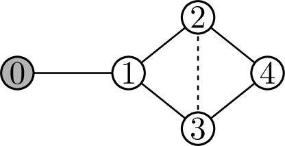
Figure 1: A graph with 5 nodes, with the grey node being the grounded one.

For the third case that $e$ connects a grounded node and a non-grounded node, we further distinguish two sub-cases: (i) subgraph $\mathcal{G}[V\backslash S]$ is connected, and (ii) subgraph $\mathcal{G}[V\backslash S]$ is disconnected. If $\mathcal{G}[V\backslash S]$ is connected, according to the result in [34], we obtain that the smallest eigenvalue of grounded Laplacian matrix grows strictly.

If $\mathcal{G}[V\backslash S]$ is disconnected, suppose that $\mathcal{G}[V\backslash S]$ consists of $r>1$ connected subgraphs. Then $\bm{\mathit{L}}_{-S}$ can be rewritten in block form as

$$\bm{\mathit{L}}_{-S}=\begin{pmatrix}\bm{\mathit{L}}_{1}&\bm{0}&\bm{0}\\ \bm{0}&\ddots&\bm{0}\\ \bm{0}&\bm{0}&\bm{\mathit{L}}_{r}\end{pmatrix}.$$ (2)

It is easy to observe that $\lambda(\bm{\mathit{L}}_{-S})=\min\{\lambda(\bm{\mathit{L}}_{1}),\dots,\lambda(\bm{\mathit{L}}_{r})\}$. According to the above analysis, when we add a new edge $e=(i,t)$ with $i\in V\backslash S$ and $t\in S$, the smallest eigenvalue of the block matrix including node $i$ will strictly increase, while the smallest eigenvalues of other blocks remain unchanged. Thus the addition of edge $e$ will lead to strict increase of the smallest eigenvalue if and only if the block matrix containing node $i$ has the unique minimum eigenvalue among all blocks.

3.2 Problem statement

Lemma 2 shows that adding an edge will increase the smallest eigenvalue of the grounded Laplacian matrix. Thus, we put forward the following eigenvalue maximization problem: How to select $k$ edges from a candidate edge set $Q$ to graph $\mathcal{G}=(V,E)$ with a grounded node set $S$, so that the smallest eigenvalue of the grounded Laplacian matrix generated by set $S$ is maximized.

When $\mathcal{G}=(V,E)$ is a small graph, $\lambda(\bm{\mathit{L}}_{-S})$ is large enough for practical applications. In what follows, we focus on large graphs, even those with more than one million nodes. In a large-scale network, if there is an edge between every pair of nodes $u\in S$ and $v\in V\backslash S$, it is easy to verify that $\lambda(\bm{\mathit{L}}_{-S})$ is not less than 1 [35], with the lower bound 1 achieved in the star graph whose center is the unique grounded node, which is already sufficiently large for application purposes and thus omitted hereafter. Finally, for a large-scale network where the number of inexistent edges linking nodes $u\in S$ and $v\in V\backslash S$ is smaller than $k$, $\lambda(\bm{\mathit{L}}_{-S})$ is generally large enough for applications [36], which we also do not consider. Therefore, in the sequel, we only treat large graphs, excluding the above two particular cases that are not significant for practical applications.

Problem 1 is a combinatorial optimization problem. To get its optimal solution, a straightforward approach is to exhaust all $\tbinom{|Q|}{k}$ possible cases for set $T$, calculate the smallest eigenvalue $\lambda(T)$ for each edge set $T$, and then output the optimal solution edge set $T^{*}$, whose addition to graph $\mathcal{G}$ leads to the largest smallest eigenvalue $\lambda(T^{*})$. The calculation of the smallest eigenvalue takes $O(n^{3})$ time for each $T$. For a sparse graph, the size of candidate edge set $Q$ is $O(n^{2})$. Thus, the computation complexity is $O\left(\tbinom{|Q|}{k}n^{3}\right)$, which is intractable even for small networks.

On the other hand, the objective function $\lambda(\cdot)$ of Problem 1 is non-submodular as stated in Theorem 3.

Theorem 3

The objective function $\lambda(\cdot):2^{Q}\rightarrow\mathbb{R}$ is a non-submodular function. That is, there exists two edge sets $A$ and $B$ obeying $A\subseteq B\subseteq Q$ and an edge $e\in Q\backslash B$, which satisfies

$$\lambda(A\cup\{e\})-\lambda(A)<\lambda(B\cup\{e\})-\lambda(B).$$ (3)

Proof.   To show its non-submodularity, consider an example of a line graph with 8 nodes in Fig. 2. Let node 0 be the grounded node, and let $A$ = $\emptyset$, $B$ = $\{(0,2)\}$ and $e$ = $(0,6)$. After simple computation, we have

$$\lambda(A)=0.0437, \lambda(A\cup\{e\})=0.1837,$$

$$\lambda(B)=0.0644, \lambda(B\cup\{e\})=0.2544.$$

Thus,

$$\lambda(A\cup\{e\})-\lambda(A)=0.14<0.19=\lambda(B\cup\{e\})-\lambda(B).$$

This finishes the proof.  $\Box$

Figure 2: A line graph with 8 nodes and 7 edges.

4 Simplification of the Problem 1

Since for each edge $e\in(S\times S)\backslash E$, $\lambda(\{e\})=\lambda(\bm{\mathit{L}}_{-S})$, indicating that adding $e$ has no influence on the smallest eigenvalue of the grounded Laplacian matrix. Thus, candidate set $Q=(V\times V)\backslash E$ in Problem 1 reduces to $(V\times(V\backslash S))\backslash E$, which, however, still has $O(n^{2})$ edges. This is one of the challenges for solving Problem 1. Below we will show that Problem 1 can be further simplified by restricting $Q$ to a subset with $O(n)$ edges, without alerting the optimal solution. The core idea is to prune a large portion of insignificant edges in $Q$.

Lemma 4

Given a graph $\mathcal{G}=(V,E)$, a grounded node set $S\subset V$, grounded Laplacian matrix $\bm{\mathit{L}}_{-S}$, a candidate edge set $Q=(V\times V)\backslash E$, for an edge $e=(i,j)\in Q$ with $i,j\in V\backslash S$, there must exist an edge $y=(z,x)\in Q$ with $z\in V\backslash S$ and $x\in S$, satisfying

$$\lambda(\{y\})\geq\lambda(\{e\}).$$ (4)

Proof.   Let $(\lambda,\bm{\mathit{u}})$ be the smallest eigen-pair of grounded Laplacian matrix $\bm{\mathit{L}}_{-S}$ for graph $\mathcal{G}=(V,E)$. When we add a new edge $e=(i,j)$, $i,j\in V\backslash S$, to $\mathcal{G}$, the grounded Laplacian matrix $\bm{\mathit{L}}_{-S}$ is perturbed with matrix $\bm{\mathit{P}}=\bm{\mathit{E}}_{i,i}+\bm{\mathit{E}}_{j,j}-\bm{\mathit{E}}_{i,j}-\bm{\mathit{E}}_{j,i}$, and the smallest eigenvalue and eigenvector $\lambda$ and $\bm{\mathit{u}}$ varies, separately, with $\mu$ and $\bm{\mathit{v}}$. Thus, we obtain

$$(\bm{\mathit{L}}_{-S}+\bm{\mathit{P}})(\bm{\mathit{u}}+\bm{\mathit{v}})=(\lambda+\mu)(\bm{\mathit{u}}+\bm{\mathit{v}}).$$ (5)

Left multiplying $\bm{\mathit{u}}^{\top}$ on both sides of the above equation gives

$$\mu=\frac{\bm{\mathit{u}}^{\top}\bm{\mathit{P}}(\bm{\mathit{u}}+\bm{\mathit{v}})}{\bm{\mathit{u}}^{\top}(\bm{\mathit{u}}+\bm{\mathit{v}})}.$$ (6)

According to matrix perturbation theory [37, 38], the small perturbation $\bm{\mathit{P}}$ on the matrix $\bm{\mathit{L}}_{-S}$ has little influence on the eigenvector $\bm{\mathit{u}}$, especially the matrix $\bm{\mathit{L}}_{-S}$ is large scaled matrix, which means $\bm{\mathit{v}}\approx\bm{0}$ [39, 40, 41, 42]. Hence,

$$\mu\approx(\bm{\mathit{u}}_{i}-\bm{\mathit{u}}_{j})^{2}.$$ (7)

In order to prove the lemma, we distinguish the following three cases.

For the first case that there exist edges $e_{1}=(i,s_{1})\in Q$, $e_{2}=(j,s_{2})\in Q$, $s_{1},s_{2}\in S$, adding $e_{1}$ or $e_{2}$ to graph $\mathcal{G}$ will lead to the grounded Laplacian matrix $\bm{\mathit{L}}_{-S}$ perturbed by $\bm{\mathit{E}}_{i,i}$ or $\bm{\mathit{E}}_{j,j}$. Let $\xi$ and $\phi$ denote, respectively, the increment of the smallest eigenvalue $\lambda$ after adding $e_{1}$ and $e_{2}$. Using a similar analysis as above, we obtain

$$\xi\approx\bm{\mathit{u}}_{i}^{2},\phi\approx\bm{\mathit{u}}_{j}^{2}.$$ (8)

Since $\bm{\mathit{u}}_{i}\geq 0$ and $\bm{\mathit{u}}_{j}\geq 0$, $\max\{\bm{\mathit{u}}_{i}^{2},\bm{\mathit{u}}_{j}^{2}\}\geq(\bm{\mathit{u}}_{i}-\bm{\mathit{u}}_{j})^{2}$ holds for any $e=(i,j)\in Q$ with $i,j\in V\backslash S$, which indicates that the maximal eigengain induced by edge $e_{1}$ or $e_{2}$ is not less than that of $e$.

For the second case only that there still exists an edge $e_{2}=(j,s_{2})\in Q$ (resp. $e_{2}=(i,s_{2})\in Q$), $s_{2}\in S$, while node $i$ (resp. $j$) connects all grounded nodes, according to [43], there exists one node $p\in V\backslash S$, and an edge $e_{3}=(p,s_{3})\in Q$, $s_{3}\in S$, such that $\bm{\mathit{u}}_{p}\geq\bm{\mathit{u}}_{i}$ (resp. $\bm{\mathit{u}}_{p}\geq\bm{\mathit{u}}_{j}$). It is easy to derive that the increment of the smallest eigenvalue induced $e_{3}$ can be approximated by $\bm{\mathit{u}}_{p}^{2}$. Hence, $\max\{\bm{\mathit{u}}_{p}^{2},\bm{\mathit{u}}_{j}^{2}\}\geq\max\{\bm{\mathit{u}}_{i}^{2},\bm{\mathit{u}}_{j}^{2}\}\geq(\bm{\mathit{u}}_{i}-\bm{\mathit{u}}_{j})^{2}$, indicating that the maximal eigengain of edges $e_{2}$ and $e_{3}$ is not smaller than that of $e$.

For the third case that both nodes $i$ and $j$ are connected to all grounded nodes, according to the result in [43], there exists one node $p\in V\backslash S$, and an edge $e_{4}=(q,s_{4})\in Q$, $s_{4}\in S$, such that $\bm{\mathit{u}}_{q}\geq\max\{\bm{\mathit{u}}_{i},\bm{\mathit{u}}_{j}\}$. Hence, $\bm{\mathit{u}}_{q}^{2}\geq(\bm{\mathit{u}}_{i}-\bm{\mathit{u}}_{j})^{2}$, indicating edge $e_{4}$ more important than $e$, with respect to increasing the smallest eigenvalue of grounded Laplacian matrix.

The analysis of the above three cases together complete our proof.  $\Box$

By Lemma 4, there are a large portion of insignificant edges in the candidate edge set $Q$, each of which links two non-grounded nodes. Thus, Problem 1 can be simplified by pruning insignificant edges, only keeping those edges in $Q$, each of which is connected to a grounded node and a non-grounded node. Also, the non-grounded node of the candidate edge decides the changes in the eigenvalue. This reduces the size of the candidate edge set $Q$ from $O(n^{2})$ to $O(n)$. Then we naturally propose a simplified version of Problem 1.

The only difference between Problems 1 and 2 is the candidate edge set $Q$. Theorem 5 provides the connection for optimal solutions between these two Problems.

Theorem 5

Any optimal solution to Problem 2 is also an optimal solution for Problem 1.

Proof.   For graph $\mathcal{G}=(V,E)$ with grounded node set $S\subset V$, let $Q_{1}=(V\times V)\backslash E$ and $Q_{2}=(S\times(V\backslash S))\backslash E$, and let $T_{1}$, and $T_{2}$ be the optimal solution of Problem 1 and Problem 2, respectively. Obviously, $\lambda(T_{2})\leq\lambda(T_{1})$ since $Q_{2}\subseteq Q_{1}$. We next prove $\lambda(T_{1})\leq\lambda(T_{2})$ by distinguishing two cases: (i) $T_{1}\subset Q_{2}$ and (ii) $T_{1}\subsetneq Q_{2}$.

For case (i) $T_{1}\subset Q_{2}$, $T_{1}$ is obviously an optimal solution to Problem 2. Thus, $\lambda(T_{2})\leq\lambda(T_{1})\leq\lambda(T_{2})$.

For case (ii) $T_{1}\subsetneq Q_{2}$, there must exist at least one edge $e_{1}=(i,j)\in T_{1}$, $i,j\in V\backslash S$. By Lemma 4, for graph $\mathcal{G}(T_{1}\backslash\{e_{1}\})=(V,E\cup T_{1}\backslash\{e_{1}\})$, there exists an edge $r_{1}=(p,t)\in Q_{1}\backslash T_{1}$, $p\in V\backslash S$, $t\in S$, satisfying $\lambda(T_{1}\cup\{r_{1}\}\backslash\{e_{1}\})\geq\lambda(T_{1})$. Define edge set $P_{1}=T_{1}\cup\{r_{1}\}\backslash\{e_{1}\}$, which is obtained from $T_{1}$ by replacing edge $e_{1}\in T_{1}$ with edge $r_{1}$. Then, we have $\lambda(P_{1})\geq\lambda(T_{1})$. Repeating this replacement at most $k$ times, we get an edge set $P_{k}\subseteq Q_{2}$, where no edge is in set $Q_{1}\backslash Q_{2}$, satisfying $\lambda(P_{k})\geq\lambda(P_{1})\geq\lambda(T_{1})$. Therefore, we have

$$\lambda(T_{2})\leq\lambda(T_{1})\leq\lambda(P_{1})\leq\lambda(P_{k})\leq\lambda(T_{2}),$$ (9)

which finishes the proof.  $\Box$

To deepen the understanding of Theorem 5, we present a simple example. Consider the graph in Fig. 1, where node 0 be the grounded node and the solid lines represent the edges in the original graph. Then, for Problem 1, the candidate edge set is $Q_{1}=\{(0,2),(0,3),(0,4),(2,3),(1,4)\}$; while for Problem 2, the candidate edge set is $Q_{2}=\{(0,2),(0,3),(0,4)\}$. We consider the case of $k=2$ for both problems. We calculate the smallest eigenvalue of the grounded Laplacian matrix after adding $2$ edges from each candidate edge set. Below we list the corresponding smallest eigenvalues for all possible sets of edges added.

$$\lambda(\{(0,2),(0,4)\})=\lambda(\{(0,3),(0,4)\})=\lambda(\{(0,2),(0,3)\})=1.120,$$

$$\lambda(\{(0,2),(2,3)\})=\lambda(\{(0,3),(2,3)\})=1.000,\lambda(\{(0,4),(2,3)\})=0.829,$$

$$\lambda(\{(0,2),(1,4)\})=\lambda(\{(0,3),(1,4)\})=1.000,\lambda(\{(0,4),(1,4)\})=0.824,$$

$$\lambda(\{(2,3),(1,4)\})=0.697.$$

Thus, the optimal solutions for Problem 2 are the edge sets $\{(0,2),(0,4)\}$, $\{(0,2),(0,3)\}$, or $\{(0,3),(0,4)\}$, which are also the optimal solutions for Problem 1.

Now, we can obtain the optimal solution Problem 1 by exhausting $\tbinom{|Q|}{k}$ possible cases for edge set $T$ in time $O(\tbinom{|Q|}{k}n^{3})$. However, this naïve method only works for very small $n$ and $k$.

5 Simple greedy algorithm

As shown above, for Problem 1 exhausting possible cases needs an exponential time. In this section, we resort to a simple greedy algorithm to approximately solve Problem 1, which is outlined in Algorithm 1. Initially, the augmented edge set $T$ is set to be empty. Then $k$ edges are iteratively selected to the augmented edge set from set $Q\setminus T$. In each iteration, the edge $e$ in candidate set with maximum $\lambda(T\cup\{e\})-\lambda(T)$ denoted by $\lambda_{T}(e)$ is chosen. The standard greedy algorithm terminates when $k$ edges are chosen to be added to $T$.

Input     :  A graph $\mathcal{G}=(V,E)$; an integer $k$; a grounded node set $S$

Output :  $T$: an edge set with $|T|=k$

1 Initialize solution $T=\emptyset$

2 Initialize candidate edge set $Q=(S\times(V\backslash S))\backslash E$

3 for $i=1$ to $k$ do

4       Compute $\lambda_{T}(e)=\lambda(T\cup\{e\})-\lambda(T)$ for each $e\in Q$

5       Select $e$ s.t. $e\leftarrow\mathrm{arg\,max}_{e\in Q}\lambda_{T}(e)$

6       Update $Q\leftarrow Q\backslash\{e\}$

7       Update solution $T\leftarrow T\cup\{e\}$

8      

return $T$

Algorithm 1 Greedy$(\mathcal{G},k,S)$

Although the objective function of Problem 2 is not submodular, the standard greedy algorithm usually has a good performance [33, 32] with a tight approximation guarantee of $(1-e^{-\gamma\alpha})/\alpha$ [33] where $\gamma$ and $\alpha$ are submodularity ratio and curvature, respectively. The effectiveness and the time complexity of Algorithm 1 are summarized in Theorem 6.

Theorem 6

Let $\gamma\in[0,1]$ and $\alpha\in[0,1]$ be submodularity ratio and curvature of the objective function of Problem 2. Then, Algorithm 1 runs in time $O(kn^{4})$, and edge set $T$ returned by Algorithm 1 satisfies

$$\lambda(T)\geq\frac{1}{\alpha}(1-e^{-\alpha\gamma})\lambda(T^{*}),$$ (10)

where

$$T^{*}=\arg\max_{T\subseteq Q,|T|=k}\lambda(T).$$

Proof.   In line 4 of Algorithm 1, for each candidate edge $e\in Q$, calculating the smallest eigenvalue $\lambda(T\cup\{e\})$ needs $O(n^{3})$ time. Since there are $O(n)$ edges in the candidate edge set, the running time of computing $\lambda_{T}(e)$ for all $e\in Q$ is $O(n^{4})$. Picking out the edge $e$ with the largest $\lambda_{T}(e)$ takes $O(n)$ time. Thus, the overall time complexity of the Algorithm 1 to pick $k$ edges is $O(kn^{4})$.

The proof of the ratio $(1-e^{-\gamma\alpha})/\alpha$ for approximation guarantee is omitted, since it is similar to that in [33].  $\Box$

It is difficult to determine the submodularity ratio $\gamma$ and the curvature $\alpha$ for the objective function of Problem 2 for general cases. However, when graph $\mathcal{G}[V\backslash S]$ is connected, we can provide a lower bound and an upper bound for $\gamma$ and $\alpha$, respectively.

Theorem 7

For a graph $\mathcal{G}=(V,E)$ with grounded node set $S\subset V$, candidate edge set $Q=(S\times(V\backslash S))\backslash E$, let $\bar{\bm{\mathit{L}}}$ be the Laplacian matrix of its subgraph $\mathcal{G}[V\backslash S]$, and let $\lambda_{2}(\bar{\bm{\mathit{L}}})$ be smallest non-zero eigenvalue of $\bar{\bm{\mathit{L}}}$. Then, when $\mathcal{G}[V\backslash S]$ is connected, for the function $\lambda(\cdot):2^{Q}\rightarrow\mathbb{R}$ of Problem 2, the submodularity ratio $\gamma$ is bounded by:

$$\gamma\geq\frac{1}{sn}\left(1-\frac{2s\sqrt{(n-s)}}{\lambda_{2}(\bar{\bm{\mathit{L}}})}\right)^{2},$$ (11)

and the curvature $\alpha$ is bounded by:

$$\alpha\leq 1-\frac{1}{sn}\left(1-\frac{2s\sqrt{(n-s)}}{\lambda_{2}(\bar{\bm{\mathit{L}}})}\right)^{2}.$$ (12)

Proof.   We first provide a lower bound for $\gamma$. To this end, for

$$\frac{\sum_{x\in T\backslash H}(\lambda(H\cup\{x\})-\lambda(H))}{\lambda(T)-\lambda(H)},\forall H\subset T\subseteq Q.$$ (13)

we provide a lower bound and an upper for its numerator and denominator, respectively.

Let $\bm{\mathit{u}}$ be the eigenvector corresponding to $\lambda(H)$ of matrix $\bm{\mathit{L}}_{-S}(H)$, and let $\bm{\mathit{u}}^{(x)}$ be the eigenvector corresponding to $\lambda(H\cup\{x\})$ of matrix $\bm{\mathit{L}}_{-S}(H\cup\{x\})$. Moreover, let $x_{i}$ be the non-grounded node incident to edge $x$. According to matrix perturbation theory [39, 41, 42], we have

$$\lambda(H\cup\{x\})-\lambda(H)=\frac{\bm{\mathit{u}}_{x_{i}}\bm{\mathit{u}}_{x_{i}}^{(x)}}{\bm{\mathit{u}}^{\top}\bm{\mathit{u}}^{(x)}}.$$ (14)

For the numerator of (13), we have

$$\sum_{x\in T\backslash H}(\lambda(H\cup\{x\})-\lambda(H))=\sum_{x\in T\backslash H}\frac{\bm{\mathit{u}}_{x_{i}}\bm{\mathit{u}}^{(x)}_{x_{i}}}{\bm{\mathit{u}}^{\top}\bm{\mathit{u}}^{(x)}}$$

$$\geq\sum_{x\in T\backslash H}\frac{\bm{\mathit{u}}_{x_{i}}\bm{\mathit{u}}^{(x)}_{x_{i}}}{\left\|\bm{\mathit{u}}\right\|_{2}\|\bm{\mathit{u}}^{(x)}\|_{2}}\geq\sum_{x\in T\backslash H}(\bm{\mathit{u}}^{(x)}_{\min})^{2}$$

$$=\sum_{x\in T\backslash H}\frac{(\bm{\mathit{u}}^{(x)}_{\min})^{2}}{(\bm{\mathit{u}}^{(x)}_{\max})^{2}}(\bm{\mathit{u}}^{(x)}_{\max})^{2}\geq\frac{1}{n}\left(1-\frac{2s\sqrt{(n-s)}}{\lambda_{2}(\bar{\bm{\mathit{L}}})}\right)^{2},$$ (15)

where $\bm{\mathit{u}}^{(x)}_{\max}$ and $\bm{\mathit{u}}^{(x)}_{\min}$ are, respectively, the largest and the smallest components of vector $\bm{\mathit{u}}^{(x)}$, and the last inequality is established based on the results in [44, 43].

For the denominator of (13), we have

$$\lambda(T)-\lambda(H)\leq\lambda(Q)-\lambda(\emptyset)\leq s.$$ (16)

Combining (5) and (16) leads to

$$\gamma\geq\frac{1}{sn}\left(1-\frac{2s\sqrt{(n-s)}}{\lambda_{2}(\bar{\bm{\mathit{L}}})}\right)^{2}\,.$$ (17)

In order to give an upper bound for $\alpha$, we provide, respectively, a lower bound and an upper for the numerator and denominator of $\frac{\lambda(T)-\lambda(T\backslash\{u\})}{\lambda(H)-\lambda(H\backslash\{u\})}$, $\forall H\subseteq T\subseteq Q,u\in H$. Utilizing an approach similar to (5) and (16), we obtain

$$\lambda(T)-f(T\backslash\{u\})\geq\frac{1}{n}\left(1-\frac{2s\sqrt{(n-s)}}{\lambda_{2}(\bar{\bm{\mathit{L}}})}\right)^{2}$$ (18)

and

$$\lambda(H)-\lambda(H\backslash\{u\})\leq\lambda(Q)-\lambda(\emptyset)\leq s,$$ (19)

both of which lead to

$$\alpha\leq 1-\frac{1}{sn}\left(1-\frac{2s\sqrt{(n-s)}}{\lambda_{2}(\bar{\bm{\mathit{L}}})}\right)^{2}.$$ (20)

This completes the proof.  $\Box$

Note that the approximation ratio $(1-e^{-\gamma\alpha})/\alpha$ characterizes the theoretical performance of the greedy algorithm, with larger $(1-e^{-\gamma\alpha})/\alpha$ corresponding to better performance. On the other hand, the approximation ratio $(1-e^{-\gamma\alpha})/\alpha$ depends on $\alpha$ and $\gamma$. It is desirable that $\alpha$ is small and $\gamma$ is large. Theorem 7 indicates that the bounds of $\gamma$ and $\alpha$ are related to $\lambda_{2}(\bar{\bm{\mathit{L}}})$. Concretely, a larger $\lambda_{2}(\bar{\bm{\mathit{L}}})$ implies a larger lower bound of $\gamma$ and a smaller upper bound of $\alpha$. Since denser graphs usually have a larger $\lambda_{2}(\bar{\bm{\mathit{L}}})$, a tighter bound for approximation ratio can be achieved on denser graphs.

6 Fast greedy algorithm

The complexity of the simple greedy algorithm 1 has been significantly reduced compared with the exhaustive search method, but it is still not applicable to large networks since it takes too much time to calculate $\lambda_{T}(e)$ for each $e\in Q$ in each iteration. On the other hand, although the approximation for $\lambda_{T}(e)$ in the proof of Lemma 4 is enough for proving the Lemma, it is not suitable for estimating the importance of two edges linking non-grounded nodes and grounded nodes, since the difference for their eigengains may be small that cannot be discriminated by this rough approximation. To overcome this issue, we use an alternative way to evaluate the upper bound for the eigengain of an edge, based on which we further give a fast approximation algorithm to solve Problem 2 in time $\tilde{O}(km)$. Note that the idea of this bound estimation method has been previously used in the literature [45, 46].

We next provide an upper bound of $\lambda_{T}(e)$ for an edge in the candidate edge $Q$ of Problem 2. For an edge $e=(t,i)\in Q$ that connects a grounded node $t\in S$ and a non-grounded node $i\in V\backslash S$, according to Cauchy’s interlacing theorem [19], we have

$$\lambda(\bm{\mathit{L}}_{-S}(T))\leq\lambda(\bm{\mathit{L}}_{-S}(T)+\bm{\mathit{E}}_{i,i})\leq\lambda((\bm{\mathit{L}}_{-S}(T))_{-i}).$$

Define $\bar{\lambda}_{T}(e)=\lambda((\bm{\mathit{L}}_{-S}(T)_{-i})-\lambda(\bm{\mathit{L}}_{-S}(T))\geq\lambda_{T}(e)$, then $\bar{\lambda}_{T}(e)$ is an upper bound of $\lambda_{T}(e)$.

To bridge the gap between matrix $\bm{\mathit{L}}_{-S}(T)$ and matrix $\bm{\mathit{L}}_{-S}(T)_{-i}$, we introduce the following matrix $\bm{\mathit{M}}_{i}$,

$$\bm{\mathit{M}}_{i}=\begin{pmatrix}(\bm{\mathit{L}}_{-S}(T))_{-i}&\bm{0}\\ \bm{0}&(\bm{\mathit{L}}_{-S}(T))_{i,i}\end{pmatrix}.$$

If there exists one node $j\in V\backslash S$ whose degree is not larger than the degree of node $i$, then by Lemma 1 the smallest eigenvalue $\lambda(\bm{\mathit{M}}_{i})$ of matrix $\bm{\mathit{M}}_{i}$ is equal to $\lambda((\bm{\mathit{L}}_{\mathcal{G}}(T))_{-i})$. Thus, as long as $i$ is not the unique node in $V\backslash S$ with the smallest degree, $\lambda(\bm{\mathit{M}}_{i})=\lambda((\bm{\mathit{L}}_{\mathcal{G}}(T))_{-i})$ always holds. In other words, there exists at most one such node $i$, whose degree is smaller than all other nodes. This situation is almost negligible, since adding a new edge from a grounded node to the node with smallest degree is often not a good choice. Thus, with a probability of at least $1-|S|/|Q|$, $\bar{\lambda}_{T}(e)=\lambda(\bm{\mathit{M}}_{i})-\lambda(\bm{\mathit{L}}_{-S}(T))$ holds. Below, we use $\lambda(\bm{\mathit{M}}_{i})-\lambda(\bm{\mathit{L}}_{-S}(T))$ instead of $\bar{\lambda}_{T}(e)$, as an upper bound of $\lambda_{T}(e)$.

The following Lemma provides an approximation of $\lambda(\bm{\mathit{M}}_{i})-\lambda(\bm{\mathit{L}}_{-S}(T))$ by using a partial derivative method [47, 48, 49].

Lemma 8

Given a connected graph $\mathcal{G}=(V,E)$, a grounded node set $S\subset V$, a candidate edge set $Q=(S\times(V\backslash S))\backslash E$, and $T\subseteq Q$, let $\bm{\mathit{L}}_{-S}(T)$ be the grounded Laplacian matrix of graph $\mathcal{G}(T)=(V,E\cup T)$, and let $(\lambda,\bm{\mathit{u}})$ be the smallest eigen-pair of matrix $\bm{\mathit{L}}_{-S}(T)$. Then, for any node $i\in V\backslash S$, we have the following approximation:

$$\lambda(\bm{\mathit{M}}_{i})-\lambda(\bm{\mathit{L}}_{-S}(T))\approx 2\bm{\mathit{u}}_{i}\sum_{j\in\mathcal{N}_{i}\backslash S}\bm{\mathit{u}}_{j}=\tilde{\lambda}_{T}(e).$$ (21)

Proof.   Notice that matrix $\bm{\mathit{M}}_{i}$ is obtained from matrix $\bm{\mathit{L}}_{-S}(T)$ by deleting the non-diagonal entries in the row and column corresponding to node $i$. To evaluate $\lambda(\bm{\mathit{M}}_{i})-\lambda(\bm{\mathit{L}}_{-S}(T))$, we use the partial derivative [47, 48, 49] to measure the change of the smallest eigenvalue $\lambda(\bm{\mathit{L}}_{-S}(T))$, caused by a nonzero non-diagonal entry at row $i$ or column $i$.

By definition of eigenvalue, we have $\lambda\bm{\mathit{L}}_{-S}(T)=\lambda\bm{\mathit{u}}$. For any $j\neq i$ and $\bm{\mathit{L}}_{-S}(T)_{i,j}\neq 0$, performing the derivative of both sides of $\lambda\bm{\mathit{L}}_{-S}(T)=\lambda\bm{\mathit{u}}$ with respect to $\bm{\mathit{L}}_{-S}(T)_{i,j}$ yields

$$\frac{\partial\bm{\mathit{L}}_{-S}(T)}{\partial\bm{\mathit{L}}_{-S}(T)_{i,j}}\bm{\mathit{u}}+\bm{\mathit{L}}_{-S}(T)\frac{\partial\bm{\mathit{u}}}{\partial\bm{\mathit{L}}_{-S}(T)_{i,j}}=\frac{\partial\lambda}{\partial\bm{\mathit{L}}_{-S}(T)_{i,j}}\bm{\mathit{u}}+\lambda\frac{\partial\bm{\mathit{u}}}{\partial\bm{\mathit{L}}_{-S}(T)_{i,j}}.$$

Left multiplying $\bm{\mathit{u}}^{\top}$ on both sides, we obtain

$$\frac{\partial\lambda}{\partial\bm{\mathit{L}}_{-S}(T)_{i,j}}=\bm{\mathit{u}}^{\top}\frac{\partial\bm{\mathit{L}}_{-S}(T)}{\partial\bm{\mathit{L}}_{-S}(T)_{i,j}}\bm{\mathit{u}}=\bm{\mathit{u}}_{i}\bm{\mathit{u}}_{j}.$$

Adding up all the partial derivative on non-diagonal nonzero element at $i$-th row and $i$-th column of matrix $\bm{\mathit{L}}_{-S}(T)$, we get an approximation of

$$\lambda(\bm{\mathit{M}}_{i})-\lambda(\bm{\mathit{L}}_{-S}(T))\approx 2\bm{\mathit{u}}_{i}\sum_{j\in\mathcal{N}_{i}\backslash S}\bm{\mathit{u}}_{j}=\tilde{\lambda}_{T}(e),$$

which is exactly (21).  $\Box$

Lemma 8 and the above analysis show that finding the maximum $\lambda_{T}(e)$ is reduced to maximizing its upper bound $\bar{\lambda}_{T}(e)$, which can be approximated by $\tilde{\lambda}_{T}(e)$ for each non-existing edge. Then, to compute $\tilde{\lambda}_{T}(e)$, the only thing left is to evaluate the smallest eigen-pair of the grounded Laplacian matrix $\bm{\mathit{L}}_{-S}$ with a low computational cost. Fortunately, this can be solved by the method in [50, 51, 52], as given in the following lemma.

Lemma 9

Given a grounded Laplacian matrix $\bm{\mathit{L}}_{-S}$ with smallest eigenvalue $\lambda(\bm{\mathit{L}}_{-S})$, there exists a nearly-linear time algorithm $\bm{\mathit{u}}=\textsc{Vector}(\bm{\mathit{L}}_{-S},\epsilon)$ with the output vector $\bm{\mathit{u}}$ and $\bm{\mathit{u}}^{\top}\bm{\mathit{L}}_{-S}\bm{\mathit{u}}$ satisfying $\bm{\mathit{u}}^{\top}\bm{\mathit{L}}_{-S}\bm{\mathit{u}}\leq(1+\epsilon)\lambda(\bm{\mathit{L}}_{-S})$. The algorithm takes $\tilde{O}(m)$ time, where $\tilde{O}(\cdot)$ hides the ${\rm poly}(\log n)$ factor.

Note that except for the approximation eigenvector $\bm{\mathit{u}}$ of matrix $\bm{\mathit{L}}_{-S}$, the algorithm $\textsc{Vector}(\bm{\mathit{L}}_{-S},\epsilon)$ in Lemma 9 can be also used to approximate $\lambda(\bm{\mathit{L}}_{-S})$ by $\bm{\mathit{u}}^{\top}\bm{\mathit{L}}_{-S}\bm{\mathit{u}}$.

Next we are in a position to propose a fast approximation algorithm for Problem 2, the pseudo-code of which is outlined in Algorithm 2, and the efficiency of which is stated in Theorem 10.

Input     :  A graph $\mathcal{G}=(V,E)$; an integer $k$; a grounded node set $S$; an error parameter $\epsilon$

Output :  $T$: an edge set with $|T|=k$

1 Initialize solution $T=\emptyset$

2 Initialize candidate edge set $Q=(S\times(V\backslash S))\backslash E$

3

4for $j=1$ to $k$ do

5       $\bm{\mathit{u}}=\textsc{Vector}(\bm{\mathit{L}}_{-S}(T),\epsilon)$

6       for each $e\in Q$ do

7             $i=$ the non-grounded node $e$ is incident to

8             Compute $\tilde{\lambda}_{T}(e)=2\bm{\mathit{u}}_{i}\sum_{t\in\mathcal{N}_{i}\backslash S}\bm{\mathit{u}}_{t}$

9            

10      Select $e$ s.t. $e\leftarrow\mathrm{arg\,max}_{e\in Q}\tilde{\lambda}_{T}(e)$

11       Update $Q\leftarrow Q\backslash\{e\}$

12       Update solution $T\leftarrow T\cup\{e\}$

13      

return $T$

Algorithm 2 Fast$(\mathcal{G},k,S,\epsilon)$

Theorem 10

The time complexity of Algorithm 2 is $\tilde{O}(km)$.

Proof.   In Algorithm 2, we first initialize the edge set $T$ and the candidate set $Q$ with size $O(n)$. Then in $k$ iterations, we calculate the eigenvector $\bm{\mathit{u}}$ associated with the smallest eigenvalue of matrix $\bm{\mathit{L}}_{-S}(T)$, which takes $\tilde{O}(m)$ time. Next, for all edges $e\in Q$, we calculate $\tilde{\lambda}_{T}(e)$, which takes $O(m)$ time. Finally, we select the edge that maximizes $\tilde{\lambda}_{T}(e)$ and add it to the edge set $T$, which need $O(n)$ time. Thus, the overall running time of Algorithm 2 is $\tilde{O}(km)$.  $\Box$

Remark 6.1

Theorem 10 shows that the time complexity of Algorithm 2 is $\tilde{O}(km)$, which is nearly linearly with respect to the number of edges. Thus, among graphs with the same number of nodes, Algorithm 2 is more efficient on sparser graphs. Specifically, for trees—the sparest class of connected graphs, the complexity of Algorithm 2 is $\tilde{O}(kn)$. As shown in the experiments Section, for those networks with similar number of nodes, Algorithm 2 runs faster on sparse networks than on dense ones.

7 Experiments

In this section, we perform experiments on a large set of real-life networks to demonstrate the effectiveness, efficiency, and scalability of our algorithms.

Table 1: Running time, smallest eigenvalues of the grounded Laplacian matrices and their ratio for Algorithms 1 and 2 on real-world networks.

Networks	Nodes	Edges	Running		Smallest Eigenvalue
			Time (s)		$(\times 10^{-4})$
			Greedy	Fast	Greedy	Fast	Ratio
Minnesota	2642	3303	9931	2.63	105	99.4	1.064
USGrid	4941	6594	20283	3.88	68.7	66.8	1.028
Bcspwr10	5300	8271	27127	5.01	69.1	67.3	1.026
RealityCall	6809	51247	37219	3.21	74.8	71.9	1.040
Eurqsa	7245	20509	61009	7.49	73.5	69.3	1.062
WHOIS	7476	56943	67233	8.04	66.1	65.8	1.003
Rajat06	10922	18061	–	11.8	–	27.9	–
Indochina2004	11358	47606	–	10.5	–	40.3	–
Amazon	91813	125704	–	179	–	0.23	–
Luxembourg	114599	119666	–	151	–	0.25	–
Sk2005	121422	334419	–	740	–	2.58	–
Caida	190914	607610	–	294	–	2.52	–
Pwtk	217891	5653221	–	1278	–	2.03	–
DBLP2010	226413	716460	–	398	–	2.17	–
TwitterFollows	404719	713319	–	270	–	1.22	–
Delicious	536108	1365961	–	729	–	0.93	–
FourSquare	639014	3214986	–	873	–	0.78	–
BerkStan	685230	7600595	–	5138	–	0.67	–
RoadNetPA	1088092	3083796	–	3001	–	0.27	–
YoutubeSnap	1134890	2987624	–	2757	–	0.44	–

7.1 Setup

Datasets. We select a large number of real-world networks of different sizes, up to one million nodes, which are publicly available in KONECT [53] and SNAP [54]. Information of networks and their nodes and edges are shown in the first three columns of Table 1. All our experiments are conducted on the largest connected component for each of these networks.

Machine Configuration and Reproducibility. Our algorithms are programmed and implemented in Julia, for convenient use of algorithm $\textsc{Vector}(\bm{\mathit{L}}_{-S},\epsilon)$ in the Julia Laplacian.jl package, which is available on https://github.com/danspielman/Laplacians.jl. The error parameter $\epsilon$ is set to be $10^{-3}$ in the experiments. All our experiments are conducted on a machine equipped with 3.5 GHz Intel i5-4690K CPU and 16G memory, using a single thread. Our source code is available on https://github.com/kedges/kedges.

Baseline Methods. We select several baselines to compare with our proposed algorithms Greedy and Fast. The baseline methods are as follows.

1. Optimum: choose $k$ edges from the candidate set $Q$, which maximize $\lambda(T)$ by exhaustive search.

2. Degree: choose $k$ edges incident to $k$ non-grounded nodes with largest degrees.

3. Eigenvector [55]: choose $k$ edges incident to $k$ non-grounded nodes with highest eigenvector centrality associated with leading eigenvalue of adjacency matrix.

4. Betweenness [56]: choose $k$ edges incident to $k$ non-grounded nodes with highest betweenness centrality.

5. Closeness [57]: choose $k$ edges incident to $k$ non-grounded nodes with highest closeness centrality.

6. $k$-center [58, 59]: choose one edge at one time to minimize the maximum distance between grounded nodes and non-grounded nodes by iterating $k$ times.

7. Eigen-approx: select $k$ edges in an iterative way. At each round, choose one edge incident to a non-grounded node with the largest component in the eigenvector $\bm{\mathit{u}}$ associated with the smallest eigenvalue for the grounded Laplacian matrix.

7.2 Effectiveness and accuracy

To exhibit the effectiveness of our two algorithms, we compare the results returned by our algorithms with the optimal solution on four small networks from KONECT [53]: Dolphins with 62 nodes and 159 edges, Tribes with 16 nodes and 58 edges, Karate with 34 nodes and 78 edges, and FirmHiTech with 33 nodes and 147 edges. For each of these four networks, we randomly select one node as the grounded node, and then add $k=1,2,\cdots,5$ edges. Due to the small scales of these networks, we can get the optimum solution within an acceptable time. We present the results in Fig. 3, which shows that both algorithms Greedy and Fast return very accurate results, which are very close to the optimum solution.

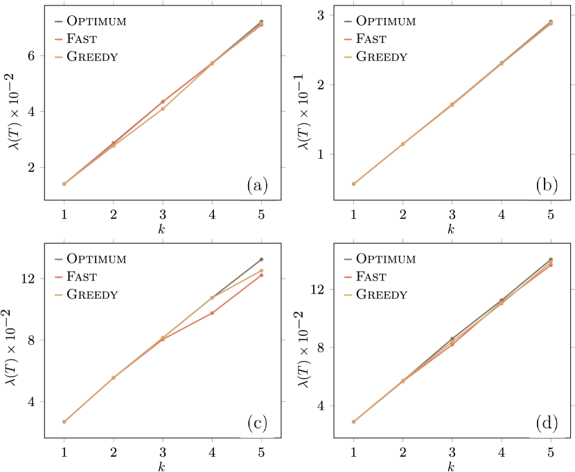
Figure 3: $\lambda(T)$ given by Fast, Greedy, and Optimum schemes for $k$ ranging from 1 to 5 on four small networks: (a) Dolphins, (b) Tribes, (c) Karate and (d) FirmHiTech.

To further show the similarity of algorithms Greedy and Fast in terms of effectiveness, we conduct experiments on six mid-sized networks in the first six rows of Table 1. For each of these six networks, we randomly select 5 nodes as grounded nodes and set $k=50$, then compute the smallest eigenvalue of the grounded Laplacian matrix after edge addition, by using algorithms Greedy and Fast. In the last three columns of Table 1, we can see the smallest eigenvalues returned by the two algorithms have little difference, since the ratio of them is close to 1.

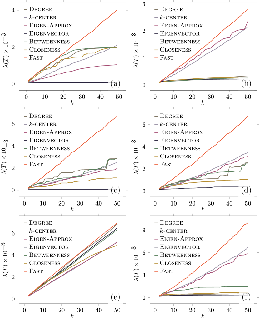
Figure 4: $\lambda(T)$ returned by Fast, Degree, Eigenvector, Betweenness, Closeness, $k$-center and Eigen-Approx, for $k$ ranging from 1 to 50 on six medium-size networks: (a) Indochina2004, (b) Rajat06, (c) USGrid, (d) Bcspwr10, (e) Eurqsa, and (f) Minnesota.

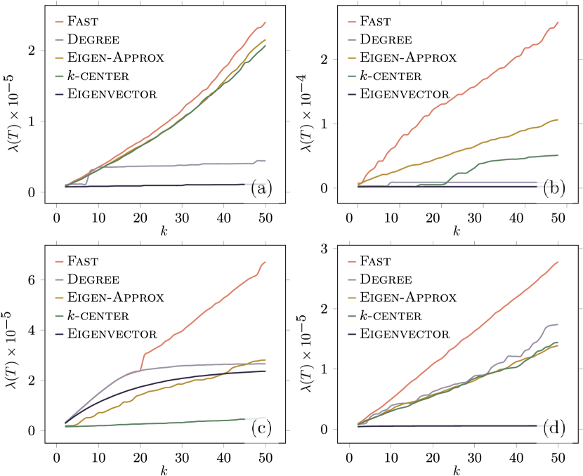
Figure 5: $\lambda(T)$ returned by Fast compared with Degree, $k$-center, Eigen-Approx and Eigenvector with $k$ ranging from 1 to 50 on four large networks: (a) Amazon, (b) Sk2005, (c) BerkStan, (d) RoadNetPA.

We also compare the results returned by algorithm Fast with those corresponding to six baseline methods on six mid-size real networks, including Degree, Eigenvector, Betweenness, Closeness, $k$-center and Eigen-Approx. For each network, we randomly select 5 nodes as grounded nodes and add $k=1,2,\cdots,50$ edges. The smallest eigenvalues returned by these 7 methods are reported in Fig. 4, which demonstrates that for Problem 2, algorithm Fast always outperforms these six baselines.

7.3 Efficiency and scalability

Theorems 6 and 10 show theoretically that the time complexity of algorithms Greedy and Fast differ greatly. Here we show experimentally that algorithm Fast runs faster than algorithm Greedy. To this end, we randomly select 5 grounded nodes and add $k=50$ edges by our two algorithms for each network listed in Table 1, and report their running time for computing the smallest eigenvalues of all augmented networks in the middle three columns of Table 1. For the networks with more than 10,000 nodes, algorithm Greedy fails due to its tremendous time cost that may be more than one day, while algorithm Fast finishes running within 2 hours even on networks with over one million nodes, indicating that Fast is scalable to large networks.

Besides our Algorithm Fast, the four baselines, Degree, $k$-center, Eigen-Approx and Eigenvector, can also quickly solve Problem 2 on large networks, the time complexity of which are $O(n)$, $O(kn)$, $\tilde{O}(km)$ and $O(m)$, respectively. However, the effectiveness of algorithm Fast is much better than the four baselines. In Fig. 5, we compare the results of algorithm Fast with those of the four baselines on four large networks with randomly selected 5 grounded nodes and varying number $k$ of adding edges. From Fig. 5, we observe that although our Fast is not the fastest, it outperforms the baseline methods.

8 Related works

In this section, we review some applications and properties of the smallest eigenvalue of the grounded Laplacian matrix, and the eigenvalue optimization problem by edge manipulation.

Applications. The notion of grounded Laplacian matrix $\bm{\mathit{L}}_{-S}$ was first proposed in [24], which arises in various practical scenarios. In particular, its smallest eigenvalue $\lambda(\bm{\mathit{L}}_{-S})$ contains a wealth of important information in different applications. For example, in leader-follower multi-agent systems describing opinion dynamics [60, 19], $\lambda(\bm{\mathit{L}}_{-S})$ characterizes the convergence speed of the states for follower agents. While in pinning control of complex networks [61, 62], $\lambda(\bm{\mathit{L}}_{-S})$ is used to measure the effectiveness of pinning control scheme [22]. Other applications for grounded Laplacian matrix include vehicle platooning [63, 64, 65], power systems [66], centrality of a group of nodes [21], and so on.

Properties of the smallest eigenvalue $\lambda(\bm{\mathit{L}}_{-S})$. Due to the vast applications of the smallest eigenvalue $\lambda(\bm{\mathit{L}}_{-S})$ for the grounded Laplacian matrix $\bm{\mathit{L}}_{-S}$, it has attracted considerable attention of many groups in recent years, in order to analyze its properties and unveil its connection with other matrices. In [43, 67, 36, 44], upper and lower bounds of $\lambda(\bm{\mathit{L}}_{-S})$ were provided; while in [22], some other properties of $\lambda(\bm{\mathit{L}}_{-S})$ were analyzed in terms of the $(|S|+1)$-th smallest eigenvalue of the Laplacian matrix $\bm{\mathit{L}}$ and the smallest degree of nodes in set $V\backslash S$. In addition, properties of $\lambda(\bm{\mathit{L}}_{-S})$ for weighted undirected graphs [68] and directed graphs [69] were also studied.

Eigenvalue optimization with edge manipulation. Addition or deletion of edges is a commonly used approach in various practical optimization problems, including the optimization problems for specific eigenvalues or their ratios of different matrices. In [70, 71] maximizing or minimizing the leading eigenvalue of the adjacency matrix was explored by adding or removing a fixed number of edges, which was shown to be NP-hard [72]. In [73], the problem of minimizing the largest eigenvalue of non-backtracking matrix [74, 75] was addressed by removing a given number of edges. In [76], the authors addressed the problem of maximizing the algebraic connectivity by creating a given number of edges, which is the smallest non-zero eigenvalue of the Laplacian matrix $\bm{\mathit{L}}$. Finally, in [77], optimizing the synchronizability was considered by adding edges, where synchronizability is measured by the ratio of the largest eigenvalue and the smallest non-zero eigenvalue of Laplacian matrix $\bm{\mathit{L}}$. Thus far, optimizing $\lambda(\bm{\mathit{L}}_{-S})$ of grounded Laplacian matrix by adding edge has not been studied. Moreover, prior methods for optimizing eigenvalues of other matrices do not apply the problem studied in this paper.

9 Conclusion

In this paper, we proposed and studied the problem of maximizing the smallest eigenvalue of the grounded Laplacian matrix $\bm{\mathit{L}}_{-S}$ of a graph $\mathcal{G}=(V,E)$ with $n$ nodes, $m\ll n^{2}$ edges, and a grounded node set $S$, by adding $k$ nonexistent edges from the candidate edge set $Q=(V\times V)\backslash E$ to graph $\mathcal{G}$. We proved that the objective function is monotonic increasing, but not submodular. Since the size of the candidate edge set is $O(n^{2})$, we simplified the problem by restricting the candidate edge set to be its proper set $(S\times(V\backslash S))\backslash E$ with $O(n)$ edges, and proved that both the simplified problem and the original problem have identical optimal solutions. We then developed two greedy algorithms to solve the problem. The first is a simple greedy algorithm, with $O(kn^{4})$ time complexity and a $(1-e^{-\gamma\alpha})/\alpha$ approximation ratio, where $\gamma$ and $\alpha$ are, respectively, the submodularity ratio and curvature of the objective function. We provided a lower bound for $\gamma$ and an upper bound for $\alpha$, when subgraph $\mathcal{G}[V\backslash S]$ is connected. The second one is a fast algorithm, with running time $\tilde{O}(km)$, where $\tilde{O}(\cdot)$ suppresses the ${\rm poly}(\log n)$ factors. Extensive experiments on real networks show that the results of our algorithms are close to each other, and both algorithms are more effective than baseline methods. Moreover, our fast algorithm is scalable to large networks with more than one million nodes. Finally, it should be mentioned that our methods and results only apply to undirected graphs. In future, we will extend or modify our techniques to directed graphs.

Declaration of competing interest

The authors declare that they have no known competing financial interests or personal relationships that could have appeared to influence the work reported in this paper.

References

- [1] M. E. J. Newman, The structure and function of complex networks, SIAM Review 45 (2) (2003) 167–256.
- [2] Y. Wang, D. Chakrabarti, C. Wang, C. Faloutsos, Epidemic spreading in real networks: An eigenvalue viewpoint, in: Proceedings of 22nd International Symposium on Reliable Distributed Systems, IEEE, 2003, pp. 25–34.
- [3] D. Chakrabarti, Y. Wang, C. Wang, J. Leskovec, C. Faloutsos, Epidemic thresholds in real networks, ACM Transactions on Information and System Security 10 (4) (2008) 1–26.
- [4] P. Van Mieghem, J. Omic, R. Kooij, Virus spread in networks, IEEE/ACM Transactions On Networking 17 (1) (2008) 1–14.
- [5] B. Bollobás, C. Borgs, J. Chayes, O. Riordan, Percolation on dense graph sequences, The Annals of Probability 38 (1) (2010) 150–183.
- [6] L. Hogben, Spectral graph theory and the inverse eigenvalue problem of a graph, Electronic Journal of Linear Algebra 14 (2005) 12–31.
- [7] J. Wu, M. Barahona, Y.-J. Tan, H.-Z. Deng, Spectral measure of structural robustness in complex networks, IEEE Transactions on Systems, Man, and Cybernetics-Part A: Systems and Humans 41 (6) (2011) 1244–1252.
- [8] R. Olfati-Saber, R. M. Murray, Consensus problems in networks of agents with switching topology and time-delays, IEEE Transactions on Automatic Control 49 (9) (2004) 1520–1533.
- [9] M. Barahona, L. M. Pecora, Synchronization in small-world systems, Physical Review Letters 89 (5) (2002) 054101.
- [10] H. Li, S. Patterson, Y. Yi, Z. Zhang, Maximizing the number of spanning trees in a connected graph, IEEE Transactions on Information Theory 66 (2) (2020) 1248–1260.
- [11] D. J. Klein, M. Randić, Resistance distance, Journal of Mathematical Chemistry 12 (1) (1993) 81–95.
- [12] H. Li, Z. Zhang, Kirchhoff index as a measure of edge centrality in weighted networks: Nearly linear time algorithms, in: Proceedings of the Twenty-Ninth Annual ACM-SIAM Symposium on Discrete Algorithms, SIAM, 2018, pp. 2377–2396.
- [13] Y. Yi, Z. Zhang, S. Patterson, Scale-free loopy structure is resistant to noise in consensus dynamics in complex networks, IEEE Transactions on Cybernetics 50 (1) (2020) 190–200.
- [14] Y. Yi, B. Yang, Z. Zhang, Z. Zhang, S. Patterson, Biharmonic distance-based performance metric for second-order noisy consensus networks, IEEE Transactions on Information Theory 68 (2) (2022) 1220–1236.
- [15] P. Tetali, Random walks and the effective resistance of networks, Journal of Theoretical Probability 4 (1) (1991) 101–109.
- [16] A. K. Chandra, P. Raghavan, W. L. Ruzzo, R. Smolensky, The electrical resistance of a graph captures its commute and cover times, in: Proceedings of the 21st Annual ACM Symposium on Theory of Computing, 1989, pp. 574–586.
- [17] Y. Sheng, Z. Zhang, Low-mean hitting time for random walks on heterogeneous networks, IEEE Transactions on Information Theory 65 (11) (2019) 6898–6910.
- [18] A. Rahmani, M. Ji, M. Mesbahi, M. Egerstedt, Controllability of multi-agent systems from a graph-theoretic perspective, SIAM Journal on Control and Optimization 48 (1) (2009) 162–186.
- [19] P. Stacy, B. Bassam, Leader selection for optimal network coherence, in: Proceedings of the 49th IEEE Conference on Decision and Control, IEEE, 2017, pp. 2692–2697.
- [20] M. Pirani, E. M. Shahrivar, B. Fidan, S. Sundaram, Robustness of leader–follower networked dynamical systems, IEEE Transactions on Control of Network Systems 5 (4) (2018) 1752–1763.
- [21] H. Li, R. Peng, L. Shan, Y. Yi, Z. Zhang, Current flow group closeness centrality for complex networks, in: Proceedings of the 2019 World Wide Web Conference, ACM, 2019, pp. 961–971.
- [22] H. Liu, X. Xu, J.-A. Lu, G. Chen, Z. Zeng, Optimizing pinning control of complex dynamical networks based on spectral properties of grounded Laplacian matrices, IEEE Transactions on Systems, Man, and Cybernetics 51 (2) (2021) 786–796.
- [23] J. A. Torres, S. Roy, A two-layer transformation for zeros analysis of networked dynamical systems, Automatica 146 (2022) 110587.
- [24] U. Miekkala, Graph properties for splitting with grounded Laplacian matrices, BIT Numerical Mathematics 33 (3) (1993) 485–495.
- [25] B. Wang, H. Liu, J. Xu, J. Liu, Pining control algorithm for complex networks, in: Proceedings of 2019 China Control Conference, IEEE, 2019, pp. 964–969.
- [26] A. Clark, B. Alomair, L. Bushnell, R. Poovendran, Leader selection in multi-agent systems for smooth convergence via fast mixing, in: Proceedings of the 51th IEEE Conference on Decision and Control, IEEE, 2012, pp. 818–824.
- [27] A. Clark, L. Bushnell, R. Poovendran, Leader selection for minimizing convergence error in leader-follower systems: A supermodular optimization approach, in: Proceedings of 10th International Symposium on Modeling and Optimization in Mobile, IEEE, 2012, pp. 111–115.
- [28] A. Clark, Q. Hou, L. Bushnell, R. Poovendran, Maximizing the smallest eigenvalue of a symmetric matrix: A submodular optimization approach, Automatica 95 (2018) 446–454.
- [29] J. Zhou, W. K. Tang, Feature-embedded evolutionary algorithm for network optimization, in: IEEE International Symposium on Circuits and Systems, IEEE, 2020, pp. 1–5.
- [30] G. Ellison, Learning, local interaction, and coordination, Econometrica: Journal of the Econometric Society (1993) 1047–1071.
- [31] C. R. MacCluer, The many proofs and applications of Perron’s theorem, SIAM Review 42 (3) (2000) 487–498.
- [32] A. Das, D. Kempe, Submodular meets spectral: Greedy algorithms for subset selection, sparse approximation and dictionary selection, in: Proceedings of the 28th International Conference on Machine Learning, Omnipress, 2011, pp. 1057–1064.
- [33] A. A. Bian, J. M. Buhmann, A. Krause, S. Tschiatschek, Guarantees for greedy maximization of non-submodular functions with applications, in: Proceedings of the 34th International Conference on Machine Learning, JMLR, 2017, pp. 498–507.
- [34] M. Fiedler, Algebraic connectivity of graphs, Czechoslovak Mathematical Journal 23 (2) (1973) 298–305.
- [35] J. Ghaderi, R. Srikant, Opinion dynamics in social networks with stubborn agents: Equilibrium and convergence rate, Automatica 50 (12) (2014) 3209–3215.
- [36] M. Pirani, S. Sundaram, On the smallest eigenvalue of grounded Laplacian matrices, IEEE Transactions on Automatic Control 61 (2) (2016) 509–514.
- [37] P. Van Mieghem, Graph Spectra for Complex Networks, Cambridge University Press, Cambridge, 2011.
- [38] A. H. Nayfeh, Perturbation Methods, John Wiley, New York, 2006.
- [39] Z. He, C. Yao, J. Yu, M. Zhan, Perturbation analysis and comparison of network synchronization methods, Physical Review E 99.
- [40] H. Liu, X. Cao, J. He, P. Cheng, C. Li, J. Chen, Y. Sun, Distributed identification of the most critical node for average consensus, IEEE Transactions on Signal Processing 63 (16) (2015) 4315–4328.
- [41] A. Milanese, J. Sun, T. Nishikawa, Approximating spectral impact of structural perturbations in large networks, Physical Review E 81.
- [42] J. G. Restrepo, E. Ott, B. R. Hunt, Characterizing the dynamical importance of network nodes and links, Physical Review Letters 97 (9) (2006) 094102.
- [43] M. Pirani, On spectral properties of the grounded Laplacian matrix, Master’s thesis, University of Waterloo (2014).
- [44] M. Pirani, E. M. Shahrivar, S. Sundaram, Coherence and convergence rate in networked dynamical systems, in: Proceedings of 54th IEEE Conference on Decision and Control, IEEE, 2015, pp. 968–973.
- [45] S. Mo, Z. Bao, P. Zhang, Z. Peng, Towards an efficient weighted random walk domination, Proceedings of the VLDB Endowment 14 (4) (2020) 560–572.
- [46] L. Torres, K. S. Chan, H. Tong, T. Eliassi-Rad, Nonbacktracking eigenvalues under node removal: X-centrality and targeted immunization, SIAM Journal on Mathematics of Data Science 3 (2) (2021) 656–675.
- [47] Y. Yi, L. Shan, H. Li, Z. Zhang, Biharmonic distance related centrality for edges in weighted networks., in: Proceedings of the 27th International Joint Conference on Artificial Intelligence, 2018, pp. 3620–3626.
- [48] M. Siami, S. Bolouki, B. Bamieh, N. Motee, Centrality measures in linear consensus networks with structured network uncertainties, IEEE Transactions on Control of Network Systems 5 (3) (2018) 924–934.
- [49] J. Kang, H. Tong, N2N: Network derivative mining, in: Proceedings of the 28th ACM International Conference on Information and Knowledge Management, ACM, 2019, pp. 861–870.
- [50] J. Batson, D. A. Spielman, N. Srivastava, S. H. Teng, Spectral sparsification of graphs: Theory and algorithms, Communications of the ACM 56 (8) (2013) 87–94.
- [51] D. A. Spielman, S.-H. Teng, Nearly linear time algorithms for preconditioning and solving symmetric, diagonally dominant linear systems, SIAM Journal on Matrix Analysis and Applications 35 (3) (2014) 835–885.
- [52] M. B. Cohen, R. Kyng, G. L. Miller, J. W. Pachocki, R. Peng, A. B. Rao, S. C. Xu, Solving SDD linear systems in nearly time, in: Proceedings of the Forty-Sixth Annual ACM Symposium on Theory of Computing, ACM, 2014, pp. 343–352.
- [53] J. Kunegis, Konect: The koblenz network collection, in: Proceedings of the 22nd International Conference on World Wide Web, ACM, 2013, pp. 1343–1350.
- [54] J. Leskovec, R. Sosič, SNAP: A general-purpose network analysis and graph-mining library, ACM Transactions on Intelligent Systems and Technolog 8 (1) (2016) 1.
- [55] B. Ruhnau, Eigenvector-centrality - a node-centrality?, Social Networks 22 (4) (2000) 357–365.
- [56] U. Brandes, A faster algorithm for betweenness centrality, Journal of Mathematical Sociology 25 (2) (2001) 163–177.
- [57] M. A. Beauchamp, An improved index of centrality, Systems Research and Behavioral Science 10 (2) (1965) 161–163.
- [58] G. Shi, K. C. Sou, H. Sandberg, K. Johansson, A graph-theoretic approach on optimizing informed-node selection in multi-agent tracking control, Physica D: Nonlinear Phenomena 267 (2014) 104–111.
- [59] T. F. Gonzalez, Clustering to minimize the maximum intercluster distance, Theoretical Computer Science 38 (1985) 293–306.
- [60] P. Barooah, J. P. Hespanha, Graph effective resistance and distributed control: Spectral properties and applications, in: Proceedings of 45th IEEE Conference on Decision and Control, IEEE, 2006, pp. 3479–3485.
- [61] X. F. Wang, G. Chen, Pinning control of scale-free dynamical networks, Physica A: Statistical Mechanics and its Applications 310 (3-4) (2002) 521–531.
- [62] X. Li, X. Wang, G. Chen, Pinning a complex dynamical network to its equilibrium, IEEE Transactions on Circuits and Systems I: Regular Papers 51 (10) (2004) 2074–2087.
- [63] B. Bamieh, M. R. Jovanovic, P. Mitra, S. Patterson, Coherence in large-scale networks: Dimension-dependent limitations of local feedback, IEEE Transactions on Automatic Control 57 (9) (2012) 2235–2249.
- [64] I. Herman, D. Martinec, Z. Hurák, M. Šebek, Nonzero bound on Fiedler eigenvalue causes exponential growth of H-infinity norm of vehicular platoon, IEEE Transactions on Automatic Control 60 (8) (2015) 2248–2253.
- [65] M. Pirani, S. Baldi, K. H. Johansson, Impact of network topology on the resilience of vehicle platoons, IEEE Transactions on Intelligent Transportation Systems.
- [66] E. Tegling, B. Bamieh, D. F. Gayme, The price of synchrony: Evaluating the resistive losses in synchronizing power networks, IEEE Transactions on Control of Network Systems 2 (3) (2015) 254–266.
- [67] M. Pirani, S. Sundaram, Spectral properties of the grounded Laplacian matrix with applications to consensus in the presence of stubborn agents, in: Proceedings of American Control Conference, IEEE, 2014, pp. 2160–2165.
- [68] S. Manaffam, A. Behal, Bounds on the smallest eigenvalue of a pinned Laplacian matrix, IEEE Transactions on Automatic Control 63 (8) (2017) 2641–2646.
- [69] W. Xia, M. Cao, Analysis and applications of spectral properties of grounded Laplacian matrices for directed networks, Automatica 80 (2017) 10–16.
- [70] C. Chen, H. Tong, B. A. Prakash, T. Eliassi-Rad, M. Faloutsos, C. Faloutsos, Eigen-optimization on large graphs by edge manipulation, ACM Transactions on Knowledge Discovery from Data 10 (4) (2016) 49:1–49:30.
- [71] C. Chen, R. Peng, L. Ying, H. Tong, Fast connectivity minimization on large-scale networks, ACM Transactions on Knowledge Discovery from Data 15 (3) (2021) 53:1–53:25.
- [72] P. Van Mieghem, D. Stevanović, F. Kuipers, C. Li, R. Van De Bovenkamp, D. Liu, H. Wang, Decreasing the spectral radius of a graph by link removals, Physical Review E 84 (1) (2011) 016101.
- [73] Z. Zhang, Z. Zhang, G. Chen, Minimizing spectral radius of non-backtracking matrix by edge removal, in: Proceedings of the 30th ACM International Conference on Information & Knowledge Management, ACM, 2021, pp. 2657–2667.
- [74] Y. Lin, W. Chen, Z. Zhang, Assessing percolation threshold based on high-order non-backtracking matrices, in: Proceedings of the 26th International Conference on World Wide Web, 2017, pp. 223–232.
- [75] Y. Lin, Z. Zhang, Non-backtracking centrality based random walk on networks, Comput. J. 62 (1) (2019) 63–80.
- [76] A. Ghosh, S. P. Boyd, Growing well-connected graphs, in: 45th IEEE Conference on Decision and Control, IEEE, 2006, pp. 6605–6611.
- [77] S. Jafarizadeh, D. Veitch, F. Tofigh, J. Lipman, M. Abolhasan, Optimal synchronizability in networks of coupled systems: Topological view, IEEE Transactions on Network Science and Engineering 8 (2) (2021) 1517–1530.