Power Spectrum in the Chaotic Regime of Axionic Blue Isocurvature Perturbations

Abstract

Large blue tilted spectral index axionic isocurvature perturbations can be produced when the axion sector is far out of equilibrium during inflation through an initial Peccei-Quinn (PQ) symmetry breaking field displacement along a nearly flat direction in the effective potential. As a companion to a previous work, we present analytic formulae for the blue isocurvature spectrum for the case of the kinetic energy density of the PQ symmetry breaking field being larger than the quartic power of the final spontaneous PQ symmetry breaking scale. It corresponds to a regime in which the nonlinearities of the classical potential become important many times during the formation of the axion isocurvature quantum perturbations leading to interesting resonant behavior. One consequence of this nonlinearity-driven resonance is the chaotic nature of the map that links the underlying Lagrangian parameters to the isocurvature amplitudes. We point out an accidental duality symmetry between the perturbation equations and the background field equations that can be used to understand this. Finally, we present two types of analytic results. The first relies on a computation utilizing an effective potential wherein fast time scale fluctuations have been integrated out. The second is grounded in a functional ansatz, requiring only a limited set of fitting parameters. Both analytic results should be useful for carrying out forecasts and fits to the data.

I Introduction

Axions offer a compelling solution to the strong CP problem (Kim:2008hd, ; Srednicki:2002ww, ; Peccei:2006as, ; Peccei:2010ed, ; DiLuzio:2020wdo, ). Due to their weak interactions with the Standard Model (SM), axions can also potentially constitute a substantial portion of the cosmological cold dark matter (CDM) Abbott:1982af ; Preskill:1982cy ; Dine:1982ah ; Kolb:1990vq ; Sikivie:2006ni ; Kawasaki:2013ae ; Marsh:2015xka . Given this dual significance of axions in both particle physics and cosmology, numerous experiments have been dedicated to their detection B_hre_2013 ; 2017 ; Ouellet_2019 ; Braine_2020 ; Gramolin_2020 ; Kwon_2021 ; Brubaker_2017 ; McAllister:2017lkb ; Alesini:2017ifp ; Alesini:2020vny ; ARIADNE:2017tdd ; Budker_2014 ; Brun_2019 ; Armengaud_2014 ; Armengaud2019 . Reviews on direct detection can be found in sources such as Ringwald:2012hr ; Redondo_2011 ; Ringwald_2014 ; Stadnik_2017 ; Carosi:2013rla ; Graham_2013 ; Agarwal_2011 ; Irastorza_2018 . In situations where the axions are spectator fields during inflation, a well-known cosmological observable called CDM-photon isocurvature perturbations can become detectable if the axions interact sufficiently weakly and do not thermalize. The generation of isocurvature perturbations by spectator axions, including its model-specific characteristics and the related observational limitations, have been extensively investigated in Kasuya1997 ; Kawasaki1995 ; Nakayama2015 ; Harigaya2015 ; Kadota2014 ; Kitajima2014 ; Kawasaki2014 ; Higaki2014 ; Jeong2013 ; Kobayashi2013 ; Hamann2009 ; Hertzberg2008 ; Beltran2006 ; Fox:2004kb ; Estevez2016 ; Kearney2016 ; Nomura2015 ; Kadota2015 ; Hikage2012 ; Langlois:2003fq ; Mollerach1990 ; Axenides1983 ; Jo2020 ; Iso:2021tuf ; Bae2018 ; Visinelli2017 ; Takeuchi:2013hza ; Bucher:2000hy ; Lu:2021gso ; Sakharov:2021dim ; Rosa:2021gbe ; Jukko:2021hql ; Chen:2021wcf ; Jeong:2022kdr ; Cicoli:2022fzy ; Koutsangelas:2022lte ; Kawasaki:2023zpd . The isocurvature spectrum studied in these cases is typically flat, and comparisons with data leads to constraints in the ($H$, $F_{a}$) parameter space Marsh:2015xka where $H$ is the inflationary Hubble scale and $F_{a}$ is the axion decay constant in equilibrium. For PQ symmetry breaking to complete before or during inflation, these parameters typically need to satisfy $F_{a}>H$. Phenomenologically, these isocurvature constraints can be naturally relaxed by introducing blue-tilted isocurvature fluctuations that can be highly suppressed on large-scales where most of the observational constraints are most severe.

Interestingly, it has been shown that axionic sector out of equilibrium dynamics during inflation can generate a large blue spectral tilt to the quantum isocurvature perturbations (Kasuya2009, ). Notably, the work of Chung:2015tha has highlighted that a detectable isocurvature signal from a linear spectator with spectral index $\gtrsim 2.4$ provides a nontrivial evidence of dynamical degrees of freedom with time-dependent masses during inflation. In a companion paper Chung:2021lfg , we have analytically and numerically computed the blue-tilted isocurvature spectrum in the model of (Kasuya2009, ) in the underdamped parametric region which produces background classical field dynamics that are only mildly resonant with the isocurvature quantum fluctuations. In this work, we focus on analytically capturing the isocurvature perturbations in strongly resonant situations in which the two Peccei-Quinn (PQ) symmetry breaking background fields cross each other many times while undergoing strongly nonlinear classical oscillations.

During these crossings, the axion perturbation amplitudes can become amplified through an effective negative mass squared effects similar to the physics of Chung:2021lfg . In our earlier study Chung:2021lfg , we focused on cases involving a maximum of one crossing after the transition where at the moment of that one crossing, the dominant force in the system is the Hubble damping term (even when the nonlinear forces driving the resonance are significant in magnitude). In this current study, as we explore situations with higher kinetic energy corresponding to quartic-potential driven forces dominating over the damping force during the crossings, we observe that the motion of the two fields becomes chaotic when the nonlinear forces dominate over the Hubble expansion rate driven damping force and the harmonic linear forces. Qualitatively, the quartic interaction within the blue axion system considered here as well as in Chung:2021lfg  can induce a chaotic behavior akin to the chaos observed in classical so-called Yang-Mills-like potentials (Carnegie_1984, ; Dahlqvist:1990zz, ; Marcinek:1994, ). Quantitatively, we observe that the field trajectory can become chaotic when the average quartic interaction energy at transition surpasses a certain threshold, $\approx O(\alpha_{{\rm Ch}})\left(F_{a}/H\right)^{4}$, where $\alpha_{{\rm Ch}}$ is an $O(1)$ threshold parameter that varies mildly with $F_{a}/H$.

This background field dynamics approximately determines the amplitude of the long wavelength quantum fluctuations because of an accidental duality between the linearized quantum mode equations and the nonlinear background field equations. This means that for the rising part of the isocurvature spectrum and the first few bumps after the resonant transition occurs, the magnitude of the isocurvature amplitude maps chaotically to the underlying Lagrangian parameters. In addition to explaining the dynamics in this strongly resonant situation, this paper presents two sets of fitting models that can be used for forecasts and data fits. One set is based on modeling the dynamical axion mass through a set of approximately square and exponential effective potentials that can be derived after integrating out the high-frequency fluctuations of the background fields. The other is a slightly simpler fitting function designed to directly match the shape and amplitude of the final isocurvature spectrum and is checked by matching with explicitly solved numerical examples.

The order of presentation is as follows. In Sec. II we provide a review of our axion toy-model introduced by Kasuya-Kawasaki in (Kasuya2009, ) and explore the dynamics of the background fields for massive underdamped fields. Moving to Sec. III, we expand upon the analysis of Chung:2021lfg  by considering massive fields that result in multiple zero-crossings of the background fields before the transition. We present an analytic expression for estimating the transition time $T_{c}$ in these cases. Next in Sec. IV, we examine the characteristics of the isocurvature power spectrum in the blue-tilted region. We accomplish this by analyzing the zero-mode ($k=0$) system and establishing appropriate matching conditions (based on an accidental duality of the mode equations) to reconcile the values with those of finite $k$ modes. This approach enables us to investigate the shape and magnitude of the isocurvature power spectrum in greater detail. We find that for massive background fields with large $O(F_{a}^{4}/H^{4})$ nonlinear interaction, the corresponding zero-mode amplitudes can show chaotic structure. We end that section by demonstrating how the duality can be used to understand the chaotic map between the Lagrangian parameters and the isocurvature amplitudes. In Sec. V we provide empirical fitting functions of the zero-mode amplitudes for the non-chaotic cases and a distribution function for the chaotic cases. In Sec. VI, we revisit the mass-model first presented in Chung:2021lfg , and expand it by applying it to several cases, fitting both the blue-tilted and oscillating regions of the spectra. Inspired by the results of the mass model, we present a simpler 7-parameter sinusoidal fitting function in Sec. VII to reduce the complexity of possible future fitting efforts. We conclude in Sec. VIII.

We present some of the finer details of our work in the following list of appendices. In App. A we estimate the non-adiabatic effects from zero-crossings and quantify their effects on the transition of the background fields. In App. B we give an approximate estimation of the phase, $\theta$, of the zero-mode solution $I_{0}$. App. C discusses the chaotic structure of the background fields. We explore one of the subdominant mass parameter dependence of the isocurvature power spectrum in App. D. Finally, in App. E we list the best-fit model parameters for the examples discussed in Sec. VII

II Massive underdamped fields

This paper is concerned with a scenario in which the complex field sector containing axion is far out of equilibrium. The key non-axion field degrees of freedom that determine the properties of the axion are $\phi_{\pm}$ fields where $\phi_{+}$ is initially displaced far from the minimum of the potential located near $F_{a}$ which is the axion decay constant. The non-equilibrium dynamics of $\phi_{\pm}$ lead to a rich set of isocurvature power spectra for the axion.

In a previous work Chung:2021lfg , we presented analytic results for axionic blue isocurvature power spectrum for the resonant underdamped cases within a specific region of the parametric space. Here, “underdamped” refers to the situation when the spectator field has a time-dependent effective mass $m$ such that $m^{2}/H^{2}>9/4$ for which the perturbation mode behaves like an underdamped oscillator. Even though $m$ is time-dependent because of its time-varying background field $\phi_{\pm}$ dependence, it happens to be approximately constant for some initial time period (specified more fully below). In Chung:2021lfg , the analysis was strictly limited to cases where the mass $m$ is minimally greater than $3H/2$ such that the background fields, $\phi_{\pm}$, cross each other close to the first zero-crossing of $\phi_{+}$ and the kinetic energy at the crossing is $\leq O(F_{a}^{4}/H^{4})$. One of the aims of this paper is to explain the dynamics for the case when $m^{2}\gg H^{2}$ (initially) which will lead to multiple zero-crossings.

In this section, we will first give a brief review of an example axion model and then discuss background field dynamics for massive fields with multiple zero-crossings before transition.

II.1 A brief review of an example axion model

In Kasuya2009 , the authors pointed out that if a PQ charged SM singlet moves along a flat direction lifted only by gravity-mediated supersymmetry (SUSY) breaking masses of $O(H)$, then the amplitude of the isocurvature fluctuations can generically have a strong blue tilt.

Consider then the chiral superfields $\Phi_{\pm,0}$ from (Kasuya2009, ) where the indices indicate the associated $U(1)_{{\rm PQ}}$ global Peccei-Quinn charges. The resulting effective potential obtained after summing up $F$-term and Kaehler induced contributions while looking along the flat direction $\Phi_{0}=0$ is

$$V\approx h^{2}|\Phi_{+}\Phi_{-}-F_{a}^{2}|^{2}+c_{+}H^{2}|\Phi_{+}|^{2}+c_{-}H^{2}|\Phi_{-}|^{2}.$$ (1)

where $h$ is a coupling coefficient, $c_{\pm}$ are positive constants, and $H$ is the inflationary Hubble scale. The parameter $c_{+}$ dominantly controls the blue isocurvature spectral index, $n_{{\rm I}}-1=3-2\sqrt{9/4-c_{+}}$ since $\Phi_{+}$ is initially displaced hierarchically larger than $\Phi_{-}$ and $F_{a}$ along the flat direction $\Phi_{+}\Phi_{-}-F_{a}^{2}=0$. Soft SUSY-breaking mass terms (${\rm TeV}$ range) are neglected as they are assumed to be much smaller than the inflationary Hubble scale $H$. This setup (even generalized away from this SUSY example) implicitly assumes that the inflation sector can be arranged to have $H\ll F_{a}$ and that the flat directions are only lifted by the quadratic terms at renormalizable level.

During inflation, the $U(1)_{{\rm PQ}}$ is broken and the $\Phi_{+}$ field rolls down along the flat direction from an initial large displacement. The magnitude of the initial displacement will eventually determine the $k$ interval over which the blue spectrum persists, and the maximum displacement of the field is of $O(M_{P})$ to have the effective field theory be under control. Such large displacements can be generically induced through supergravity induced effects from a UV completion of the theory. The Nambu-Goldstone boson associated with a linear combination of the phases of the two fields is recognized as the axion. In particular, with the parameterization

$$\Phi_{\pm}\equiv\frac{\varphi_{\pm}}{\sqrt{2}}\exp\left(i\frac{a_{\pm}}{\sqrt{2}\varphi_{\pm}}\right)$$ (2)

where $\varphi_{\pm}$ and $a_{\pm}$ are real, the axion is

$$a=\frac{\varphi_{+}}{\sqrt{\varphi_{+}^{2}+\varphi_{-}^{2}}}a_{+}-\frac{\varphi_{-}}{\sqrt{\varphi_{+}^{2}+\varphi_{-}^{2}}}a_{-}$$ (3)

while the heavier partner is ignored as it is not dynamically important. Using the scalings defined as

$$\phi_{\pm}\equiv\Phi_{\pm}\frac{h}{H}$$ (4)

$$F=hF_{a}/H$$ (5)

$$\xi(\phi_{+},\phi_{-})\equiv\phi_{+}\phi_{-}-F^{2}$$ (6)

and

$$T\equiv tH,$$ (7)

the background equations of motion with the interaction force $\xi\phi_{\pm}$ can be written as

$$\ddot{\phi}_{+}(T)+3\dot{\phi}_{+}(T)+c_{+}\phi_{+}+\xi(\phi_{+},\phi_{-})\phi_{-} =0$$ (8)

$$\ddot{\phi}_{-}(T)+3\dot{\phi}_{-}(T)+c_{-}\phi_{-}+\xi(\phi_{+},\phi_{-})\phi_{+} =0$$ (9)

for motions of $\Phi_{\pm}$ where the background $\Phi_{\pm}$ does not change its phase. The associated mode equation for the fluctuations $I_{\text{$\pm$}}\equiv\delta a_{\pm}/2$ (see Chung:2016wvv for details) is

$$\left(\partial_{T}^{2}+3\partial_{T}\right)I+\left(\frac{Ka(0)}{a(T)}\right)^{2}I+\tilde{M}^{2}I=0$$ (10)

where

$$K\equiv\frac{k}{a(0)H}$$ (11)

is the scaled physical wave vector at the initial time of $\phi_{+}$ rolling defined as $T=0$, the vector $I=(I_{+},I_{-})$ contains the quantum axion fluctuation information, and the mass matrix is

$$\tilde{M}^{2}(T)\equiv\left(\begin{array}[]{cc}c_{+}&F^{2}\\ F^{2}&c_{-}\end{array}\right)+\left(\begin{array}[]{cc}\phi_{-}^{2}(T)&0\\ 0&\phi_{+}^{2}(T)\end{array}\right).$$ (12)

Hence, at the Lagrangian level, the effective set of parameters governing the background and linearized perturbation dynamics is $\{c_{+},c_{-},F\equiv hF_{a}/H\}$. As will be detailed in Sec II.2, the initial condition of the background fields will be restricted to a two parameter family $\left(\phi_{+}(0),\dot{\phi}_{+}(0)\right)$ with the $\phi_{-}(0)$ and $\dot{\phi}_{-}(0)$ fixed according to the constraint that the fields are sitting on the flat direction. The boundary conditions for the mode functions will be Bunch-Davies (BD).

The expression for the isocurvature fluctuations during inflation can be written as

$$\Delta_{s}^{2}(t,\vec{k})\approx 4\omega_{a}^{2}\frac{k^{3}}{2\pi^{2}}I^{\dagger}\left(\begin{array}[]{cc}r_{+}^{2}&0\\ 0&r_{-}^{2}\end{array}\right)I$$ (13)

for

$$r_{\pm}\equiv\sqrt{\frac{\phi_{\pm}^{2}(t)}{(\phi_{+}^{2}(t)+\phi_{-}^{2}(t))^{2}\theta_{+}^{2}(t_{i})}}$$ (14)

where $\omega_{a}$ is the ratio of axion energy density to the dark matter fraction today and $\theta_{+}(t_{i})$ is the initial axion angle. The quantity $\omega_{a}$ is sensitive to the assumption of whether or not the axion contained in $I$ is the QCD axion. For specificity, the reader can assume that this is the QCD axion and refer to the formula of the misalignment scenario dark matter fraction given in Chung:2016wvv , although this paper is largely insensitive to this assumption. Hence, as far as the CDM-photon isocurvature is concerned, there is one more parameter of $\omega_{a}^{2}/\theta_{+}^{2}(t_{i})$. In summary, as far as the power spectrum is concerned, what we will focus in on this paper is a 3 (Lagrangian) + 2 (initial conditions) + 1 (initial misalignment angle) parameter model.

II.2 Resonance and transition

In Chung:2021lfg , we derived analytic expressions for the isocurvature power spectrum in the underdamped cases. These cases occur when the mass-squared term $c_{+}H^{2}$ of the $\phi_{+}$ field slightly exceeds $9H^{2}/4$ and the kinetic energy of the background fields $\phi_{\pm}$ is within specific parametric bounds when at their crossing. To analyze these scenarios, the authors in Chung:2021lfg  employed a combination of perturbative and non-perturbative methods, due to the deviation of the fields from the flat direction described in Eq. (6) which leads to non-adiabatic effects when the background fields are approaching the potential minimum. This deviation is caused by the $\phi_{+}$ field tending to zero while the total energy of the system is $O(F^{4}$). Consequently, there is a significant increase in the kinetic energy during the field crossing. In comparison to an overdamped scenario, the authors in Chung:2021lfg  discovered that this substantial kinetic energy at the crossing leads to diverse spectral shapes with multiple bumps. Moreover, the underdamped cases examined in Chung:2021lfg   exhibited an amplification of the isocurvature spectral amplitude by at least $O(30)$ relative to the massless plateau.

More explicitly, consider the zeroth order perturbed solution of Eqs. (8) and (9) which is valid in the limit $\sqrt{\phi_{-}/\phi_{+}}\ll 1$ where we assume that $\phi_{+}$ field rolls down along the flat direction from an initial displacement much greater than $F$ (typically $O(M_{P}/H)$). Hence, we can approximate $\phi_{+}$ as

$$\phi_{+}(T)\approx\phi_{+}^{(0)}(T) =\phi_{+}(0)e^{-\frac{3}{2}T}\sec(\varphi)\cos(\omega T-\varphi)$$ (15)

where

$$\omega=\sqrt{c_{+}-9/4},$$ (16)

$$\tan\varphi\equiv\frac{3/2+\epsilon_{0}}{\omega},$$ (17)

and

$$\epsilon_{0}\equiv\frac{\dot{\phi}_{+}(0)}{\phi_{+}(0)}$$ (18)

describes the initial velocity. Note that underdamped cases imply that $c_{+}>9/4$. The matching order $\phi_{-}(T)$ solution is given as

$$\phi_{-}(T)\approx\phi_{-}^{(0)}(T)=\frac{F^{2}}{\phi_{+}^{(0)}}.$$ (19)

In Chung:2021lfg , the analysis was carried out by defining a new parameter

$$\alpha \equiv\frac{\left|\partial_{T}\phi_{+}^{(0)}(T_{z})\right|}{F^{2}}$$ (20)

$$=\omega\frac{\phi_{+}(0)}{F^{2}}\,\sec\varphi\,e^{-3/2T_{z}}$$ (21)

that characterizes the kinetic energy of the underdamped background fields close to a zero-crossing. Here, $T_{z}$ is the zero of the $\phi_{+}^{(0)}$ field defined by

$$\phi_{+}^{(0)}\left(T_{z}\right)=0.$$ (22)

Figure 1: Plot highlighting the background field dynamics for $c_{+}=4.533$ where the $\phi_{+}$ field undergoes multiple zero-crossings before transitioning at approximately $T_{c}\approx 9.4$. The remaining Lagrangian parameters are set at $F_{a}/H=20.2$, $c_{-}=0.5$, $\epsilon_{0}=0$ and $\phi_{+}(0)/H=3.32\times 10^{8}$.

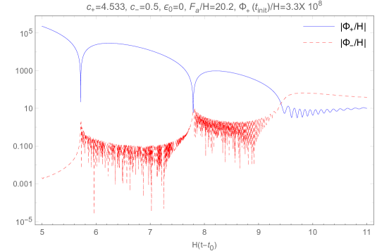
As the $\phi_{+}$ field approaches zero, it intersects with the $\phi_{-}$ field. The number of these crossings is uniquely determined by the value of $c_{+}$ through $\omega$ defined in Eq. (16). Fig. 1 shows the rolling down of the background fields for a fiducial value of $c_{+}=4.533$ that exhibits multiple zero-crossings of $\phi_{+}^{(0)}$ occurring at times $T_{z}\approx 1.56,\;3.63,\;5.7,\;7.79,\;\mbox{and }9.87$. The plot is obtained for an illustrative fiducial set $P_{A}$ of parameters that we will often use throughout this paper:

$$P_{A}\equiv\{F=20.2,\,c_{-}=0.5,\,\epsilon_{0}=0,\,\phi_{+}(0)=0.1M_{p}/H\}.$$ (23)

At each crossing, we can assess the influence of the $\phi_{-}$ field on $\phi_{+}$ by evaluating the force $\xi\phi_{-}$. These forces can induce displacements of $\phi_{+}$ towards the “steep” direction of the potential (perpendicular to the flat direction), where $\xi$ is significant. This in turn causes strong oscillatory behavior of both $\phi_{+}$ and the order unity coupled $\phi_{-}$. Thus, during each crossing at a time $T_{{\rm cross}}$ when $\phi_{+}(T_{{\rm cross}})=\phi_{-}(T_{{\rm cross}})$, we can express the effective coupling force $f_{+}$ on $\phi_{+}$ as follows:

$$f_{+}(T_{{\rm cross}})=-\xi\phi_{-}|_{T_{{\rm cross}}}$$ (24)

whose magnitude measures the deviation of $\phi_{+}$ from the flat direction trajectory or the zeroth order solution given in Eq. (15). This deviation is a sufficient condition for the force in the steep direction to be significant. Hence, we define resonant transition time $T_{c}$ as the first $T_{{\rm cross}}$ that satisfies the following two conditions:

$$\left.f_{+}\right|_{T=T_{c}}\gtrsim O(0.1)\left|\ddot{\phi}_{+}(T_{c})\right|$$ (25)

and

$$|\dot{\phi}_{+}(T_{{\rm c}})|\gtrsim\alpha_{{\rm L}}F^{2}.$$ (26)

The first of the conditions ensure sufficient coupling force from $\phi_{-}$ such that $\phi_{+}$ deviates significantly from the unperturbed solution $\phi_{+}^{(0)}$ while the second condition here is required for $\phi_{+}$ to oscillate with an amplitude such that the kinetic energy is sufficiently large, $O(F^{4})$. When the above two conditions are satisfied, the two background fields oscillate with a frequency of $O(F)$. We call this situation “resonance”. In Chung:2021lfg , we chose $\alpha_{{\rm L}}\approx 0.2$ as the threshold for resonance. For the fiducial example presented in Fig. 1, the transition occurs at $T_{c}\approx 9.5$ which is close to the $5$th zero-crossing, $T_{z,5}=9.87$. Note that the force $f_{+}$ is directly proportional to the amplitude of $\phi_{-}$, and from Eq. (19), we see that $\phi_{-}$ becomes $O(F)$ when $\phi_{+}\sim O(F)$. Therefore, the transition typically occurs in the vicinity of a zero-crossing of $\phi_{+}^{(0)}$. The moment of transition serves as a pivotal time in the coupled dynamics of the background fields. It marks the point in time when the axion begins to make a dynamical transition to a massless final state. From an observational perspective, it defines the wavenumber, $k_{c}$, which corresponds to the location of the cutoff where the isocurvature spectrum smoothly departs from a blue-tilted power law.

Unlike the case presented in Fig. 1, the analysis and findings described in Chung:2021lfg  were focused on $c_{+}$ values for which the background fields $\phi_{\pm}$ undergo a transition close to the first zero-crossing of the $\phi_{+}^{(0)}$ field. Additionally, the parameter $\alpha$ was constrained within approximate bounds of $[0.2,1)$. However, for larger $c_{+}$ values, the condition specified in Eq. (25) may not be fulfilled at the first zero-crossing. In the next section, we will estimate the $n$th zero-crossing point which is closest to the transition $T_{c}$ and hence satisfies the conditions outlined in Eqs. (25) and (26). Then, by determining the value of $\alpha$ at this zero-crossing, we can effectively characterize the dynamics of the background fields after the transition.

III Estimation of the $T_{z}$ closest to $T_{c}$

As discussed above and illustrated in Fig. 1, in case of underdamped scenarios, the background fields $\phi_{\pm}$ intersect each other near each zero-crossing of $\phi_{+}^{(0)}$ until the transition occurs at time $T_{c}$. The zero-crossings of the zeroth order solution $\phi_{+}^{(0)}$ in Eq. (15) are given by the expression

$$T_{z,j}=\frac{1}{\omega}\left(\left(j-\frac{1}{2}\right)\pi+\varphi\right)$$ (27)

where $j$ gives us the location of the $j$th zero-crossing. Using Eq. (20), we define the quantity $\alpha_{j}$ at each $T_{z,j}$ as

$$\alpha_{j}=\omega\frac{\phi_{+}(0)}{F^{2}}e^{-\frac{3}{2}T_{z,j}}\sec(\varphi).$$ (28)

From Fig. 1 we observe that close to each $T_{z,j}$, the two background fields cross each other at $T_{{\rm cross},j}$. The amplitude of the fields at each $T_{{\rm cross},j}$ is controlled by the parameter $\alpha_{j}$. In Appendix. A, we demonstrate that a higher value of $\alpha_{j}$ results in a greater incoming velocity of the $\phi_{+}$ field, resulting in a smaller crossing amplitude $\phi_{\pm}\left(T_{{\rm cross},j}\right)$. Since the force $f_{+}$ as defined in Eq. (24) is proportional to the amplitudes of the two fields at the crossing, there exists an upper limit on the value of $\alpha_{j}$ for the transition to occur while satisfying the condition described in Eq. (25). Thus, for $\alpha_{j}$ higher than the upper limit, the field amplitudes are too small at the crossings and correspondingly the force $f_{+}$ isn’t significant to cause the transition.

To estimate the value of $T_{z,j}$ which is closest to the transition, we consider the first condition stated in Eq. (25) and perform an integration in a small neighborhood around $T_{c}$. By integrating this condition, we determine the smallest value of $j$ that satisfies the condition and corresponds to the occurrence of the transition. Thus, we obtain

$$\int_{T_{c}-\delta T_{2}}^{T_{c}+\delta T_{1}}dT\left(\phi_{+}\phi_{-}^{2}-F^{2}\phi_{-}\right)\gtrsim O(0.1)\left|\left.\dot{\phi}_{+}\right|_{T_{c}-\delta T_{2}}^{T_{c}+\delta T_{1}}\right|.$$ (29)

Since the fields must cross before the zero-crossing of $\phi_{+}$, we choose the lower and upper boundaries as $T_{c}-\delta T_{2}=T_{s}$ and $T_{c}+\delta T_{1}=T_{z,j}$ where

$$T_{s}=T_{z,j}-2\epsilon_{j}$$ (30)

for $\epsilon_{j}=1/\left(F\sqrt{\alpha_{j}}\right)$. In Chung:2021lfg , this choice of $\epsilon_{j}$ was defined to be approximately when the deviation of the $\phi_{-}$ from $\phi_{-}^{(0)}$ of Eq. (19) is roughly 10$\%$. Since we have $F\gg 1$, the time interval $\epsilon_{j}$ is far less than unity for values of $\alpha_{j}\gg 1$, and thus we can expand $\phi_{\pm}$ within the interval of integration as

$$\phi_{-}(T) \approx\phi_{-}^{(0)}(T_{s})+\dot{\phi}_{-}^{(0)}(T_{s})(T-T_{s})$$ (31)

$$\phi_{+}(T) \approx\phi_{+}^{(0)}(T)\approx\alpha_{j}F^{2}\left((T-T_{z,j})-\frac{3}{2}(T-T_{z,j})^{2}\right).$$ (32)

In Appendix A of Chung:2021lfg , it was shown explicitly that neglecting higher order derivatives for the $\phi_{-}$ field near transition ($T\sim T_{c}-O(2/F)$) leads to a much better approximation and hence we restrict ourselves to a first-order expansion for $\phi_{-}$. Upon substitution into Eq. (29) we get

$$\int_{T_{s}}^{T_{z}}\left(\phi_{+}^{(0)}\phi_{-}^{2}-F^{2}\phi_{-}\right)dt \gtrsim O(0.1)\left|\left.\dot{\phi}_{+}^{(0)}\right|_{T_{s}}^{T_{z,j}}\right|$$ (33)

$$\frac{F^{3}\left(1944+1458F\sqrt{\alpha_{j}}+384F^{2}\alpha_{j}+35F^{3}\alpha_{j}^{3/2}\right)}{60\sqrt{\alpha_{j}}\left(3+F\sqrt{\alpha_{j}}\right)^{4}} \gtrsim O(0.1)\;6F\sqrt{\alpha_{j}}$$ (34)

$$\frac{7F^{2}}{12\alpha_{j}}-\frac{3F}{5\alpha_{j}^{3/2}}+O\left(\frac{1}{F\alpha_{j}^{5/2}}\right) \gtrsim O(0.1)\;6F\sqrt{\alpha_{j}}$$ (35)

which when solved in the limit $F\gg 1$ yields

$$\alpha_{j}\lesssim\left(\frac{7F}{72\,O(0.1)}\right)^{\frac{2}{3}}.$$ (36)

We note that the upper limit in the right hand side (RHS) of Eq. (36) is sensitive to the choice of an $O(0.1)$ number. By comparing with the numerical results, we choose a value of $0.07$, and thus obtain

$$\alpha_{j}\lesssim 1.244\times F^{\frac{2}{3}}$$ (37)

as the upper limit on the value of $\alpha_{j}$ for the transition to occur close to the zero-crossing at $T_{z,j}$. Hence, using Eqs. (20), (25) and (36) we infer that the background fields transition when

$$\left|\dot{\phi}_{+}^{(0)}\right|_{T_{z,j}}=\alpha_{j}F^{2}\lesssim F^{\frac{2}{3}+2}.$$ (38)

Eq. (38) is isomorphic to Eq. (25). Since $F\gg 1$, our assumption that $\alpha_{j}\gg 1$ above Eq. (32) is justified. For instance, if $F=20$ we obtain the upper bound as $\alpha\approx 9$ which also satisfies the second condition given in Eq. (26). We will now estimate the smallest value of $j$ that satisfies the condition in Eq. (38) for a given $c_{+}$ and initial conditions. Defining the upper bound as $\alpha_{{\rm max}}=1.244F^{\frac{2}{3}}$ from Eq. (36) and $j_{c}$ as the $j$th index corresponding to the zero-crossing closest to transition $T_{c}$, we require that

$$\alpha_{j_{c}} <\alpha_{{\rm max}}$$ (39)

$$\omega\frac{\phi_{+}(0)}{F^{2}}e^{-\frac{3}{2}T_{z,j_{c}}}\sec(\varphi) <\alpha_{{\rm max}}$$ (40)

$$T_{z,j_{c}} >\frac{-2}{3}\ln\left(\frac{\alpha_{{\rm max}}F^{2}}{\omega\phi_{+}(0)\sec(\varphi)}\right)$$ (41)

$$\frac{1}{\omega}\left(\left(j_{c}-\frac{1}{2}\right)\pi+\varphi\right) >\frac{-2}{3}\ln\left(\frac{\alpha_{\max}F^{2}}{\omega\phi_{+}(0)\sec(\varphi)}\right)$$ (42)

$$j_{c} >\frac{1}{2}-\frac{1}{\pi}\left(\frac{2\omega}{3}\ln\left(\frac{\alpha_{{\rm max}}F^{2}}{\omega\phi_{+}(0)\sec(\varphi)}\right)+\varphi\right).$$ (43)

Therefore, the zero-crossing $T_{z,j_{c}}$ closest to the transition $T_{c}$ is given by the expression

$$T_{z,j_{c}}=\frac{1}{\omega}\left(\left(\text{Ceiling}\left[\frac{1}{2}-\frac{1}{\pi}\left(\varphi+\frac{2\omega}{3}\ln\left(\frac{\alpha_{{\rm max}}F^{2}}{\omega\phi_{+}(0)\sec(\varphi)}\right)\right)\right]-\frac{1}{2}\right)\pi+\varphi\right)$$ (44)

which has a limiting behavior

$$\lim_{\omega\gg 1}T_{z,j_{c}} \approx\frac{\pi}{\omega}\text{Ceiling}\left[-\frac{2\omega}{\pi 3}\ln\left(\frac{\alpha_{{\rm max}}F^{2}}{\omega\phi_{+}(0)\sec(\varphi)}\right)-\frac{1}{2}\right].$$ (45)

Figure 2: Plot of $T_{z,j_{c}}$ with respect to $\omega$ providing an approximate time at which the background fields transition for different values of $c_{+}$. The curve is generated using Eq. (44) and exhibits discontinuous curves corresponding to increasing integer values of $j=j_{c}$ starting with $j_{c}=1$ for the first branch corresponding to $\omega\lesssim 0.4$. Once $T_{z,j_{c}}$ is known for given Lagrangian parameters, an analytical estimate for the location of the transition $T_{c}$ can be made using Eq. (50). The above plot is obtained using the standard fiducial set $P_{A}$ given in Eq. (23).

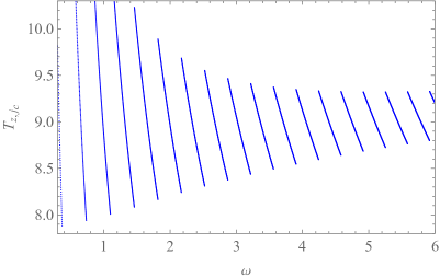
In Fig. 2 we plot $T_{z,j_{c}}$ with respect to $\omega$ using Eq. (44). The corresponding value of the parameter $\alpha$ at $T_{z,j_{c}}$ is

$$\alpha_{c}=\omega\frac{\phi_{+}(0)}{F^{2}}e^{-\frac{3}{2}T_{z,j_{c}}}\sec(\varphi)$$ (46)

where we introduce the index $c$ on $\alpha$ to distinguish it from other non-transition $\alpha_{j}$ values. Note that for the rest of our discussion, $\alpha_{c}$ refers to the value at $T_{z,j_{c}}$ close to transition $T_{c}$. In Fig. 3 we show the value of $\alpha_{c}$ as a function of $\omega$ where the individual discontinuous curves are bounded from above by the upper bound $\alpha_{{\rm max}}$ given in Eq. (36), while the lower bound in each successive branch increases with $\omega$. The plot highlights distinct monotonic branches in the $\omega(c_{+})-\alpha_{c}$ phase space. Within a branch, such as the range $c_{+}\in[3.5,4.21]$, $\alpha_{c}$ exhibits a monotonically increasing behavior, reaching the maxima defined in Eq. (36), before abruptly transitioning to the next branch.

Figure 3: Plot highlighting different monotonic branches in the $\omega(c_{+})-\alpha_{c}$ phase space showing the $c_{+}$ dependence of $\alpha_{c}$ for standard fiducial set $P_{A}$ defined in Eq. (23). Each of the branches in the above figures corresponds to an increasing value of $j_{c}$ where $j_{c}=1$ for the first branch starting from $c_{+}=9/4$ and similarly $j_{c}=4$ for the branch where $\omega\in[1.11,1.4]$ corresponding to $c_{+}\in[3.5,4.21]$.

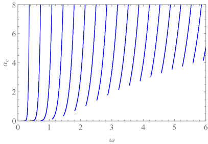
This can be understood by recalling that, for the background fields to transition, the condition described in Eq. (25) must be fulfilled. As $\alpha$ increases, the LHS in Eq. (25) decreases while the RHS increases. Consequently, for sufficiently large values of $\alpha$, the left-hand side can drop below the threshold required to meet the condition, prompting the fields to transition at the next zero-crossing (succeeding branch). This occurs as they dissipate enough total kinetic energy through Hubble friction, leading to a reduction in the value of $\alpha$.

Furthermore, we observe that for cases with larger values of $c_{+}$, the value of $\alpha$ at transition is larger than $O(1)$. This will have intriguing implications when we study the isocurvature power spectrum in Sec. IV for the cases where the background fields tend to exhibit chaotic behavior.

To summarize the above analysis, as the parameter $c_{+}$ increases, the background fields undergo more frequent oscillations with shorter time periods. Since the system of background fields must lose sufficient energy before transition, the number of zero-crossings before transition increases with $c_{+}$. Close to each zero-crossing, the fields momentarily cross each other. If the field velocity, characterized by the parameter $\alpha$, is sufficiently small at a given crossing $T_{{\rm cross},j_{c}}$ while still satisfying Eq. (25), then the two fields are said to transition. This imposes an upper bound on the value of $\alpha$ for the transition to occur.

In the above analysis, we have focused on the adiabatic approximation, neglecting the nonadiabatic effects originating from all zero-crossings ($j<j_{c}$) prior to transition. The analysis and examples considered in Chung:2021lfg  had $T_{c}$ close to the first zero-crossing ($j_{c}=1$) and therefore nonadiabatic effects due to previous zero-crossings $T_{z,j}$ were absent. These nonadiabatic oscillations can be understood as rapid transient (homogeneous) oscillations of the $\phi_{-}$ field, generated at $T_{z,j}$, due to the quartic interaction term, $(\phi_{+}\phi_{-}-F^{2})^{2}$, in the reduced Lagrangian. Consequently, the homogeneous component, $\phi_{-}\approx\phi_{-,{\rm Tr}}$, oscillates rapidly with an effective frequency controlled by $\phi_{+}$ and an amplitude approximately proportional to $\alpha_{j}^{-3/4}$. In Appendix A we provide a detailed derivation of $\phi_{-,{\rm Tr}}$.

However, if $T_{z,j}$ is at least two e-folds time interval prior to $T_{c}$, with the corresponding value of $\alpha_{j}$ much larger than unity, the nonadiabatic effects from previous zero-crossings corresponding to values of $\alpha_{j}\gg\alpha_{\max}$ do not induce significant changes in the mode functions. This is because the dynamical effects differing from that of a constant mass decays as

$$\frac{\Delta I_{\pm}}{I_{\pm}}\sim O\left(\frac{1}{\alpha_{j}}\right)\sim O\left(e^{-\frac{3}{2}(T_{c}-T_{z,j})}\right).$$ (47)

These $\alpha_{j}^{-1}$ effects are the non perturbative resonant oscillations that occur at each crossing of the background fields.

For cases where a previous zero-crossing has occurred within about two e-folds time interval of $T_{c}$ (applicable to $c_{+}\gtrsim 5$), the nonadiabatic effects from the zero-crossing at $T_{z,j_{c}-1}$ can have a significant impact. The rapid oscillations of $\phi_{-,{\rm Tr}}$ lead to an increase in the effective mass of the $\phi_{+}$ field, resulting in a mass-squared function $m_{+}^{2}\approx c_{+}+\phi_{-}^{2}$ of the $\phi_{+}$ field that can exceed $c_{+}$ for $T_{z,j_{c}-1}<T<T_{c}$. As a consequence, the zero-crossing $T_{z,j_{c}}$ corresponding to $T_{c}$ is modified and occurs slightly earlier than predicted by Eq. (44) due to an increased frequency of $\phi_{+}$ during the time-interval $T_{z,j_{c}-1}<T<T_{c}$.

In Appendix A we analytically solve the equation of motion (EoM) for the $\phi_{+}$ field in the time-region $T_{z,j_{c}-1}<T<T_{c}$, taking into account the finite nonadiabatic effects arising due to the UV oscillations of $\phi_{-}$ field. We derive a general expression for the deviation of the $\phi_{+}$ field from the zeroth order solution $\phi_{+}^{(0)}$. This modified analytic solution for the $\phi_{+}$ given in Eq. (152) is useful in predicting the location of the next zero-crossing at $T_{z,j_{c}}$. Consequently we can state that the next zero-crossing at $T_{z,j_{c}}$ occurs at

$$T_{z,j_{c}}-T_{z,j_{c}-1}=\frac{\pi}{\omega}-\Delta T\left(A_{j_{c}-1}\right)$$ (48)

where $\Delta T\left(A_{j_{c}-1}\right)$ is a function of the amplitude of $\phi_{-,{\rm Tr}}$ at $T_{z,j_{c}-1}$. We can obtain an estimate for $\Delta T$ by solving the transcendental equation corresponding to $\phi_{+}(T_{z,j_{c}})=0$ using the analytic solution of $\phi_{+}$ given in Eq. (152).

For resonant underdamped cases where $\alpha_{c}\gtrsim\alpha_{{\rm L}}\approx 0.2$, the transition time $T_{c}$ can be estimated using the expression

$$T_{c}\approx T_{z,j_{c}}-\frac{0.7}{F\alpha_{c}}\qquad\alpha_{c}\gtrsim\alpha_{{\rm L}}$$ (49)

given in Sec. 4 of Chung:2021lfg . For a broad range of $\alpha_{c}$ values including non-resonant cases, we propose the following fitting formula:

$$T_{c}\approx T_{z,j_{c}}-\left(-2.396+\frac{9.8047}{1+1.112\left(F\alpha_{c}/20.2\right)-6.013\left(F\alpha_{c}/20.2\right)^{0.5}+7.935\left(F\alpha_{c}/20.2\right)^{0.25}}\right)\qquad\alpha_{c}\gtrsim 10^{-4}$$ (50)

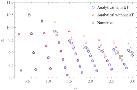
where $T_{z,j_{c}}$ is obtained from Eq. (48). In Fig. 4 we plot the transition time, $T_{c}$, as a function of $\omega$ for fiducial set $P_{A}\equiv\{F=20.2,\,c_{-}=0.5,\,\epsilon_{0}=0,\,\phi_{+}(0)=0.1M_{p}/H\}$. We compare our analytic estimates obtained from the expressions given in Eq. (50) with the numerical values and find an accuracy $\gtrsim 90\%$. We observe that the non-adiabatic effects generated from the previous zero-crossing must be taken into account using the $\Delta T$ correction for $\omega\gtrsim 1.5$ corresponding to $c_{+}\gtrsim 4.5$. Note that these corrections are important when $\alpha_{c}\lesssim 1$ since the corresponding non-adiabatic effects from a previous zero-crossing scale as $A_{j_{c}-1}^{2}\sim O\left(\alpha_{j_{c}-1}^{-1/2}F^{3}\right)$ where

$$\alpha_{j_{c}-1}^{-1/2}\approx\left(\alpha_{c}e^{\frac{3\pi}{2\omega}}\right)^{-1/2}\propto\alpha_{c}^{-1/2}$$ (51)

where we remind the reader that $\alpha_{c}\equiv\alpha_{j_{c}}$ is the value of the $\alpha$ parameter at the zero-crossing $T_{z,j_{c}}$.

Figure 4: Plot showing the transition time $T_{c}$ as a function of $\omega$ for the standard fiducial set $P_{A}\equiv\{F=20.2,\,c_{-}=0.5,\,\epsilon_{0}=0,\,\phi_{+}(0)=0.1M_{p}/H\}$. For comparison, we plot the values using our analytical estimate from Eq. (50) with and without the $\Delta T$ correction for $T_{z,j_{c}}$ as described in Eq. (48). We observe that our analytical prediction including the $\Delta T$ correction matches with the numerical values with an accuracy $\gtrsim 90\%$. As noted in the main text, the $\Delta T$ correction becomes significant for $\omega\gtrsim 1.5$ which corresponds to a time-interval $\pi/\omega\lesssim 2$ e-folds between the adjacent zero-crossings and hence the non-adiabatic corrections described in App. A cannot be neglected. We find that these corrections are important when $\alpha_{c}\lesssim 1$ since the corresponding non-adiabatic effects from a previous zero-crossing scale as $\approx e^{\frac{-\pi}{\omega}}\alpha_{c}^{-1/2}$.

In Chung:2021lfg , the authors observed that the location of the first bump in the isocurvature power spectrum is approximately $k_{{\rm first-bump}}\approx 2Ha(0)\exp\left(T_{c}\right)$. Since $T_{c}\approx T_{z,j_{c}}+O(1/F)$ for $\alpha_{c}>\alpha_{{\rm L}}$, we find that for $c_{+}\gg 9/4$,

$$T_{c}\approx T_{z,j_{c}} \sim O\left(\text{$\frac{2}{3}\ln\left(\frac{\phi_{+}(0)}{F^{8/3}}\right)$}\right).$$ (52)

Therefore, the location of the first bump or the cutoff scale from a blue-tilted part of the spectrum to a flat plateau is related to the hierarchy between the initial displacement of the $\phi_{+}$ field and the $f_{PQ}\equiv F_{a}$ scale. In order to hide the isocurvature spectrum at large CMB scales, we require a large hierarchy or displacement along the flat direction. This is a generic requirement for the blue axion models where the blue index is generated during the slow roll along a flat direction. Conversely, it is possible to move the cutoff scale towards lower $k$ values by choosing a larger $F$, while keeping all other cosmological parameters such as the number of inflationary efolds $N_{{\rm inf}}$, $\phi_{+}(0)$, $H$, and reheating temperature $T_{{\rm RH}}$ fixed. The estimation of $T_{c}$, given in this section, allows us to predict the cutoff scale $k_{c}$ for the high-blue isocurvature spectrum.

In the next section, we will discuss the isocurvature power spectrum in the blue-tilted region for for the massive $c_{+}$ cases and present plots highlighting the $\alpha_{c}$ dependence of the final isocurvature amplitudes.

IV Isocurvature power spectrum in the blue region

For the axion model considered in this work, the isocurvature power spectrum generated during inflation is evaluated using the expression given in Eq. (13) by solving the coupled differential system in Eq. (10) for the associated mode fluctuations $\delta a_{\pm}/2\equiv I_{\text{$\pm$}}$. Since we are considering massive underdamped cases where $c_{+}>9/4$, the isocurvature power spectrum generically has a high-blue spectral index $\text{Re}\left[n_{{\rm I}}\right]\approx 4$. This blue-tilted region of the power spectrum extends to all modes $k<k_{c}$ that exit the horizon well before the transition of the background fields $\phi_{\pm}$ at time $T_{c}$, where the cutoff scale $k_{c}$, is associated with transition $T_{c}$, and marks the region in the spectrum where the power spectrum begins to settle into a scale-invariant massless plateau.

In Chung:2021lfg , the authors uncovered that for specific cases where the value of the parameter $\alpha_{c}$ at transition is $\gtrsim O(0.1)$, there is a significant increase in the kinetic energy during the field crossing. This substantial kinetic energy at the transition leads to nonadiabatic effects during the period when the background fields are approaching the potential minimum that results in diverse spectral shapes with multiple bumps/oscillations. Moreover, for the cases covered in Chung:2021lfg , the authors found that these resonant non-adiabatic effects for the underdamped cases lead to an amplification of at least $O(30)$ relative to the massless plateau. In summary, the isocurvature power spectrum for the massive underdamped fields consists of two regions: a blue-titled spectrum for $k\lesssim k_{c}$ and a region with multiple bumps for $k>k_{c}$ that eventually settles to a scale-invariant massless plateau. The cutoff scale $k_{c}$ that separates these two regions of the spectrum is a function of $T_{c}$.

IV.1 Zero-mode $I_{0}$

Because the superhorizon inhomogeneous modes $I_{\pm}(k)$ behave similarly as the background fields (as explained below), the superhorizon modes in principle only need to be solved until the horizon crossing and matched to the background fields, similar to what happens to curvature perturbation variables during the quasi-dS era. This simplifies the computation if one has access to an accurate computation of background field solutions. The inhomogeneous modes $I_{\pm}(k)$ can be solved trivially for $T<T_{c}$ for the small $k$ region analytically, which allows this matching program to be efficient for the rising blue part of the power spectrum characterized by a simple power law. The main nontriviality is to argue that despite the nonadiabaticities of the mass matrix that affects the mode equations for $T>T_{c}$, we can compute the functional behavior of the power spectrum (to a matching condition-dependent $r_{a}$ accuracy). This will allow us to obtain an expression for the approximate $k$ dependence of the power spectrum for long wavelength modes. Furthermore, because of the accidental duality that exists between the superhorizon modes and the background fields, we will be able to semi-quantatively explain the chaotic map between the Lagrangian parameters such as $c_{+}$ and the isocurvature amplitude.

Let us begin with the mode function governed by Eq. (10) for the axion model. After normalizing with the BD adiabatic vacuum, the mode function for $T<T_{c}$ when $\phi_{+}^{2}\gg F^{2}$ is given as

$$\lim_{K\exp(-T)\gg 1}I(K,T\ll T_{c})\approx I^{(\mathrm{early})}(K,T)\equiv\left(\frac{e^{-T}}{2a(0)}\right)^{3/2}\sqrt{\frac{\pi}{H}}e^{-\omega\frac{\pi}{2}+i\frac{\pi}{4}}H_{i\omega}^{(1)}\left(Ke^{-T}\right)\left[\begin{array}[]{c}1\\ 0\end{array}\right]+O\left(\frac{F^{2}}{\phi_{+}^{2}(T)}\right)\left[\begin{array}[]{c}0\\ 1\end{array}\right]$$ (53)

where $\omega=\sqrt{c_{+}-9/4}$, $a(0)$ is the scale factor at a chosen initial time $T_{0}=0$, and the normalized wave vector $K$ is defined in Eq. (11). Note that the normalization here is different from $1/\sqrt{2ka^{2}}$ by another factor of $1/\sqrt{2}$. Here we emphasize that the BD boundary condition is aligned along the lightest normalized real eigenvector, $e_{1}$, of the mode mass-matrix $\tilde{M}^{2}$ which was defined in Eq. (12). In terms of a parameter, $\lambda=F^{2}/\phi_{+}^{2}$, the lightest eigenvector of $\tilde{M}^{2}$ in the limit $\lambda\ll 1$ can be given as

$$e_{1}(T)=\left[\begin{array}[]{c}1\\ 0\end{array}\right]-\lambda\left[\begin{array}[]{c}0\\ 1\end{array}\right]+O(\lambda^{2}).$$ (54)

while the heavier eigenvector, $e_{2}$, is

$$e_{2}(T)=\left[\begin{array}[]{c}0\\ 1\end{array}\right]+\lambda\left[\begin{array}[]{c}1\\ 0\end{array}\right]+O(\lambda^{2}).$$ (55)

Hence, Eq. (53) can be equivalently written as

$$I^{(\mathrm{early})}(K,T\ll T_{c})\approx\left(\frac{e^{-T}}{2a(0)}\right)^{3/2}\sqrt{\frac{\pi}{H}}e^{-\omega\frac{\pi}{2}+i\frac{\pi}{4}}H_{i\omega}^{1}\left(Ke^{-T}\right)e_{1}(T)$$ (56)

which has a peculiar normalization in that in the $K\rightarrow\infty$ limit, it has an extra power of $1/\sqrt{2}$ coming from a choice of axion normalization and a physically irrelevant extra overall minus sign coming from a phase choice. We note that Eq. (56) is an approximation that holds only when the contribution from the heavier mode can be neglected. The most general expression for $I(K,T)$ valid at all times can be written as

$$I(K,T)=y_{1}(K,T)e_{1}(T)+y_{2}(K,T)e_{2}(T)$$ (57)

where $y_{1,2}$ are the corresponding mode functions in the instantaneous eigenstate basis. In Chung:2021lfg  the authors demonstrated that as the background fields approach transition at $T_{c}$, substantial mode mixing occurs. Through their analysis, they revealed that the heavy-mode mixing is most significant when the hierarchy between the lightest and the heaviest mass eigenvalues is minimal. As a result, the expression in Eq. (56) is generically invalid as $T\rightarrow T_{c}$. However, when the background fields have settled to the minima, the mode function asymptotes to

$$I(K,T_{\infty})\approx y_{1}(K,T_{\infty})e_{1}(T_{\infty})$$ (58)

where $e_{1}(T_{\infty})$ corresponds to the Goldstone mode of the axionic system.

Let us now consider modes that exit the horizon at $\mathcal{T}_{K}<T_{c}$ which is defined to be when

$$K^{2}\exp\left(-2\mathcal{T}_{K}\right)=r_{a}(c_{+}-2)$$ (59)

where $r_{a}\sim 0.1$ represents the accuracy with which one wants to estimate the amplitude. Because of Eq. (56), we know

$$y_{1}(K,\mathcal{T}_{K})\approx\left(\frac{e^{-\mathcal{T}_{K}}}{2a(0)}\right)^{3/2}\sqrt{\frac{\pi}{H}}e^{-\omega\frac{\pi}{2}+i\frac{\pi}{4}}H_{i\omega}^{(1)}\left(Ke^{-\mathcal{T}_{K}}\right).$$ (60)

One can also check that $y_{2}(K,\mathcal{T}_{K})$ term is comparatively negligible for $\mathcal{T}_{K}<T_{c}$.Now let us consider Eq. (10) with $k=0$ which describes a mode a priori distinct from any physical modes because $k=0$ is always outside of the horizon:

$$\left(\partial_{T}^{2}+3\partial_{T}\right)I_{0}+\tilde{M}^{2}I_{0}=0.$$ (61)

Note that the variable change

$$I_{0}\rightarrow I_{0}^{(\mathrm{dual})}\equiv(f_{0}\phi_{+},-f_{0}\phi_{-})$$ (62)

maps the zero-mode system in Eq. (61) to the background field EoMs in Eqs. (8) and (9) for a nonvanishing constant $f_{0}$. This is a type of an accidental duality in which the background equations become identical to the perturbation equations even though the background equations are nonlinear. Although $I$ that we seek appearing in Eq. (57) is fundamentally different from $I_{0}^{\mathrm{(dual)}}$ since $I_{0}^{\mathrm{(dual)}}$ is real up to a time-independent phase, we know that one linear combination of $I_{0}$ and $I_{0}^{*}$ can be made to equal $I_{0}^{\mathrm{(dual)}}$. This, in particular, means that if $\phi_{\pm}$ solutions exhibit exponential sensitivity to parameters, then $I_{0}$ will as well. Such exponentially sensitive parametric dependence will be presented later in this section.

We impose boundary conditions for Eq. (61) for the zero-mode $I_{0}$ at a time $T_{0}\ll T_{c}$ along the direction of the lightest eigenvector $e_{1}$, following a similar phase expression as shown in Eq. (56):

$$I_{0}(T_{0}) =e^{-\left(3/2+i\omega\right)T_{0}}e_{1}$$ (63)

$$\left.\partial_{T}I_{0}\right|_{T=T_{0}} =-\left(3/2+i\omega\right)e^{-\left(3/2+i\omega\right)T_{0}}e_{1}$$ (64)

which is not the same as the BD condition since these modes are already outside of the horizon. On the other hand, unlike the dual $I_{0}^{\mathrm{(dual)}}$ which can be made real by dividing by $f_{0}$, the zero mode $I_{0}(T)$ here is complex with a time-dependent phase just like $I(K,T)$ which means that $I_{0}^{*}$ will be an independent solution once $I_{0}$ is known owing to the real valued nature of the differential equation system. At the horizon exit time $\mathcal{T}_{K}<T_{c}$, the zero-mode near time $\mathcal{T}_{K}$ can be given by the expression

$$I_{0}(T)\approx e^{-\left(3/2+i\omega\right)T}e_{1}(T)\,\,\,\,\,\,\,\,\,\,\,\,\,\mbox{ near }T\sim\mathcal{T}_{K}$$ (65)

because the heavier mode contribution can still be neglected at that time. The $k$-dependent mode function $I(K,\mathcal{T}_{K}$) can be written as

$$y_{1}(K,T)e_{1}(T)\approx c_{1}(K)I_{0}(T)+c_{2}(K)I_{0}^{*}(T)$$ (66)

for $T\sim\mathcal{T}_{K}$. Note that we have conveniently avoided any contribution from the heavier eigenmode $e_{2}$ at $\mathcal{T}_{K}$ by ensuring that $\lambda(\mathcal{T}_{K})\ll 1$. The coefficients $c_{1,2}(K)$ are obtained by using Eqs. (54), (60), (65), and (66). For $T>T_{c}>\mathcal{T}_{K}$, the complete $I_{0}(T)$ solution incorporates all significant interactions arising from the mixing of nontrivial heavier mode such that $I(T\geq\mathcal{T}_{K})$ can be evaluated as

$$I(K,T\geq\mathcal{T}_{K})=c_{1}(K)I_{0}(T)+c_{2}(K)I_{0}^{*}(T)$$ (67)

where we obtain the matched coefficients $c_{1,2}(k)$ to be

$$c_{1}(k)=\left(1+i\right)2^{-2-i\omega}\left(\frac{1}{a(0)}\right)^{3/2}\left(\frac{k}{a(0)H}\right)^{i\omega}\exp\left(-\pi\omega/2\right)\sqrt{\frac{\pi}{H}}\frac{\left(1+\coth\left[\omega\pi\right]\right)}{\Gamma\left(1+i\omega\right)}+O(r_{a})$$ (68)

$$c_{2}(k) = \left(1-i\right)2^{-2+i\omega}\left(\frac{1}{a(0)}\right)^{3/2}\left(\frac{k}{a(0)H}\right)^{-i\omega}\exp\left(-\pi\omega/2\right)\frac{1}{\sqrt{\pi H}}\Gamma(i\omega)+O(r_{a})$$ (69)

where $k=Ka(0)H$. Since we require that $\mathcal{T}_{K}<T_{c}$, the above method is valid for $k$ modes that satisfy

$$\ln\left[\frac{k}{a(0)H\sqrt{r_{a}c_{+}}}\right]<T_{c}.$$ (70)

Numerically we found an accuracy up to $90\%$ for modes $K\lesssim 0.35\exp\left(T_{c}\right)$. Note that $|c_{1,2}|^{2}$ is independent of $k$ because $i\omega$ is imaginary.

The axion isocurvature power spectrum in Eq. (13) can be expressed in terms of the zero-mode by expanding

$$I^{\dagger}\left(\begin{array}[]{cc}r_{+}^{2}&0\\ 0&r_{-}^{2}\end{array}\right)I$$

in terms of $I_{0}$ evaluated at a time $T=T_{\infty}$. At $T_{\infty}$, the Goldstone theorem is satisfied and the $\tilde{M}^{2}$ mass-matrix yields one massless and one massive eigenvalue where the massless mode corresponds to the axion. Therefore, for the normalized massless eigenvector $\psi_{0}$ at the end ($T\rightarrow T_{\infty}$):

$$\tilde{M}^{2}\psi_{0}=0$$ (71)

or more explicitly

$$\psi_{0}=\frac{1}{\sqrt{c_{+}+c_{-}}}\left(\begin{array}[]{c}-\sqrt{c_{-}}\\ \sqrt{c_{+}}\end{array}\right).$$ (72)

Since as $T\rightarrow T_{\infty},\leavevmode\nobreak\ \tilde{M}^{2}\psi_{0}\rightarrow 0$, we find

$$I_{0}(T)\approx\left(\mathcal{N}e^{i\theta}+\mathcal{A}e^{-3T}\right)\psi_{0}$$ (73)

where $\mathcal{A}$ is a complex number, $\mathcal{N}$ and $\theta$ are real numbers independent of $k$. In terms of $\psi_{0}$,

$$\left(\begin{array}[]{cc}r_{+}^{2}&0\\ 0&r_{-}^{2}\end{array}\right)_{T=T_{\infty}}=C\left[\frac{c_{-}+c_{+}}{c_{-}}\psi_{0}\psi_{0}^{\dagger}+\sqrt{\frac{c_{+}}{c_{-}}}\sigma_{x}\right]$$ (74)

for a constant $C$ that depends upon $F$, $\theta_{+}$ and $c_{\pm}$ and where $\sigma_{x}$ is a Pauli matrix. Using the above definitions, the isocurvature power spectrum for $k$ modes that satisfy Eq. (70) is given as

$$\Delta_{s}^{2}(k)\approx\mathcal{N}^{2}\left(4\frac{\omega_{a}^{2}}{\theta_{+}^{2}}\right)\left(\frac{k^{3}}{2\pi^{2}}\right)\frac{\sqrt{c_{+}c_{-}}(c_{+}^{2}+c_{-}^{2})|c_{1}(k)e^{i\theta}+c_{2}(k)e^{-i\theta}|^{2}}{(c_{+}+c_{-})^{3}(F_{a}^{2}-\sqrt{c_{-}c_{+}}H^{2})}$$ (75)

where the $k$-independent real coefficients $\mathcal{N}$ and $\theta$ cannot be analytically computed in the present approach.

   

   

Figure 5: In the top row, we plot the ratio $|m_{1}/m_{2}|$ of the lightest over heaviest mass eigenvalues of the mass-matrix $\tilde{M}^{2}$ for two fiducial cases with $c_{+}$ values $2.3533$ and $2.345$, both at $F_{a}/H=20.2$ and $c_{-}=0.5$. A substantial hierarchy between the lighter and heavier eigenvalues renders the impact of the mode mixing and the contribution from the heavier mode $e_{2}$ negligible. Examining the two plots in the top row, we observe that the heavy mode mixing is most pronounced for $c_{+}=2.3533$ (left) compared to $c_{+}=2.345$ (right). In the bottom row, we compare the isocurvature power spectrum obtained from solving the $k$-dependent mode equations as given in Eq. (10) (solid markers) with our approximation (solid and dashed curves) given in Eq. (75) constructed from the numerical solution to the zero-mode equation. The solid red (dashed black) curves are plotted using the numerical value of $\theta$ (approximation $\theta=-\omega T_{c}$). By construction, the zero-mode solution incorporates all significant nontrivial interactions arising from the heavy mode mixing. Note that the slope of the power spectrum in the $k$-range shown above is $\approx 2.6$, signaling the nontrivial correction from the sinusoid in log $k$.

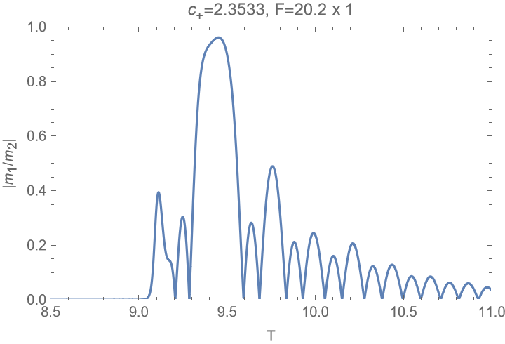
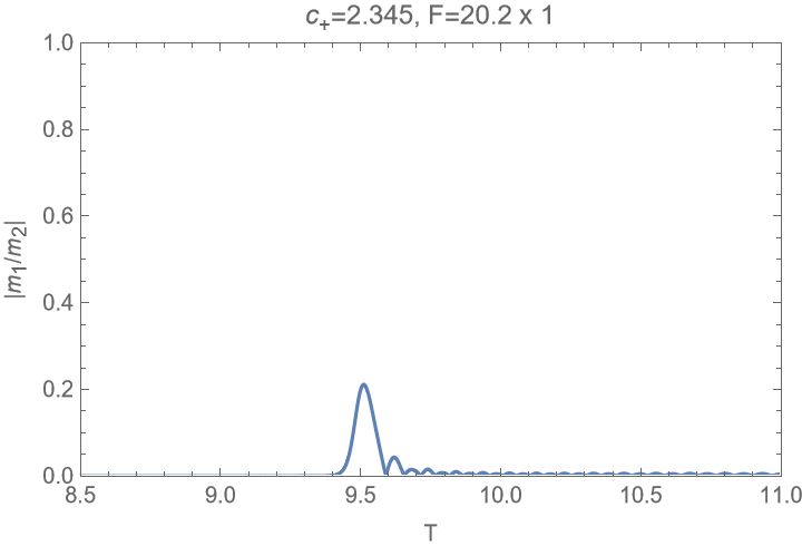
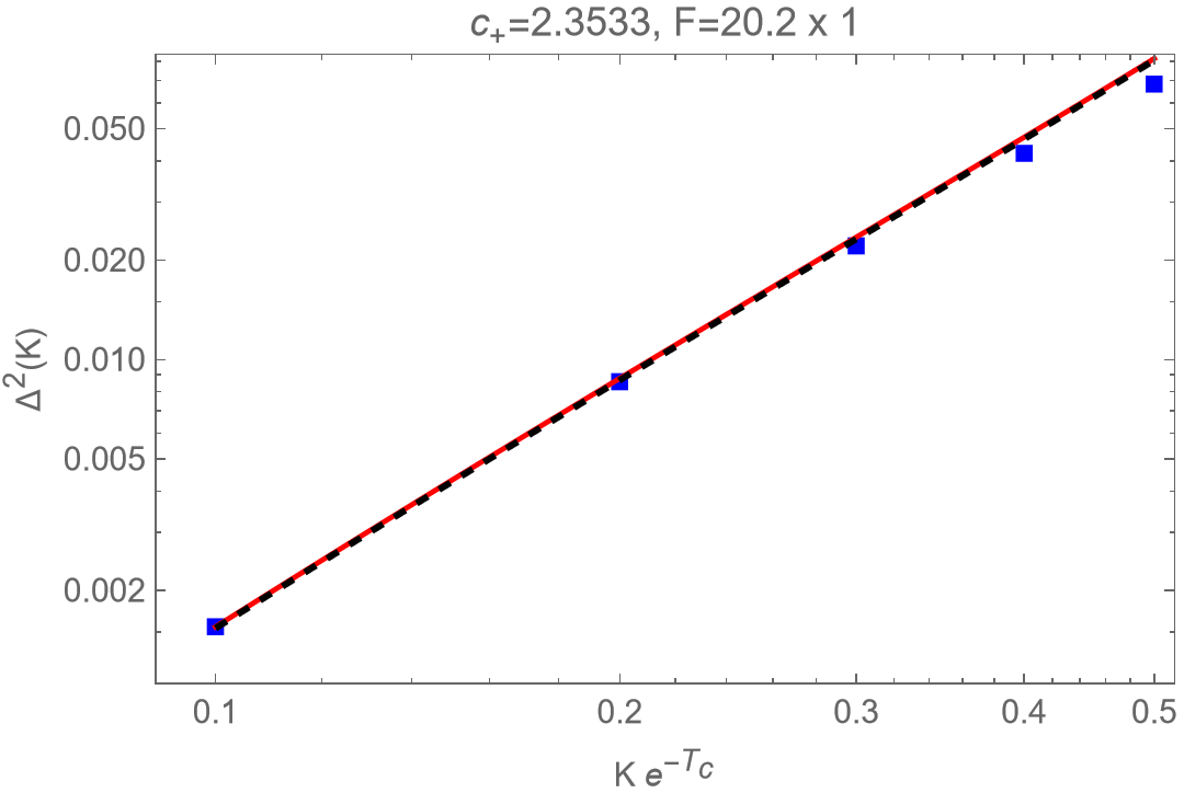
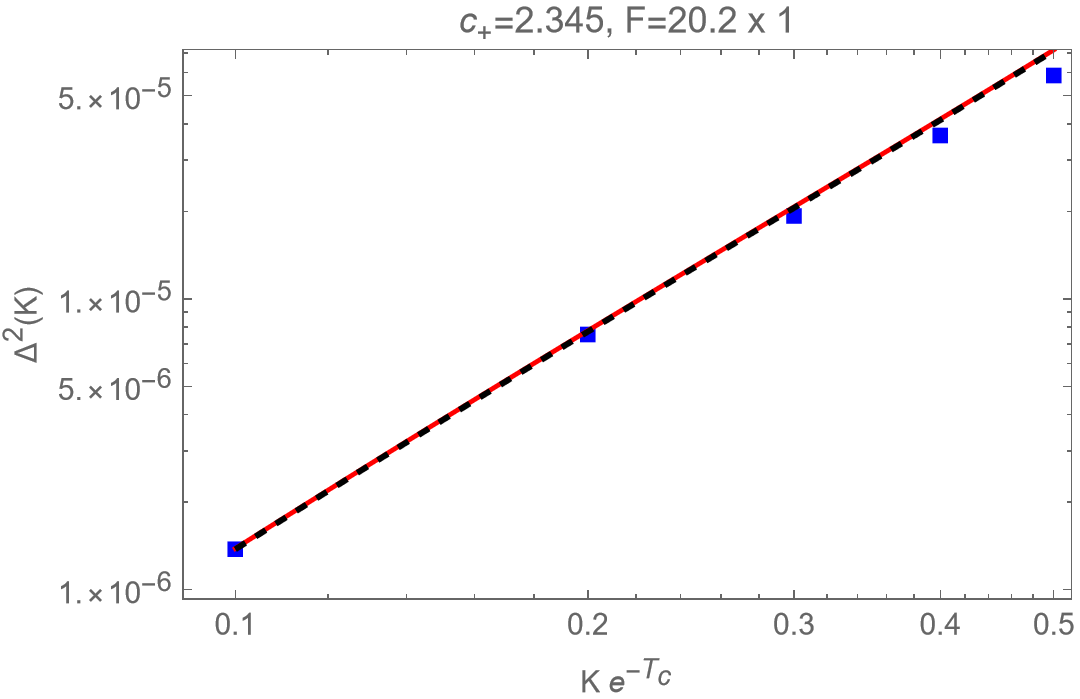
The power spectrum is directly proportional to the square of the amplitude $\mathcal{N}$ of the scalar mode $z$. The $c_{1}^{*}(k)c_{2}(k)$ have only logarithmic $k$ dependence, which makes this solvable situation having an approximately $k^{3}$ dependence in the long wavelength limit as long as $c_{1}(k)e^{i\theta}+c_{2}(k)e^{-i\theta}$ does not vanish. In that sense, the prediction in this parametric region ($k^{3}$ part of the spectrum with small sinusoidal oscillations in log $k$) is not particularly interesting in $k$ dependence. However, the amplitude computation is nontrivial, and that is what is captured by the intricate numerical computation of $|I_{0}|$. Through the factorization of the zero-mode in Eq. (73), the normalization of the isocurvature power spectrum at late times as given by the expression in Eq. (75) now depends upon the mode amplitude $\mathcal{N}$, while the dependence on the wavenumber $k$ is determined by the $\theta$ parameter. In Appendix B we show that $\theta$ can be approximated as $-\omega T_{c}.$ Consequently, we can conveniently eliminate $\theta$ when evaluating the power spectrum using Eq. (75).

In Fig. 5, we compare the isocurvature power spectrum obtained from solving the $k$-dependent mode equations as outlined in Eq. (10) (blue markers) with our approximation given in Eq. (75) constructed from the zero-mode solution. Through the plots, we highlight that the zero-mode solution $I_{0}$, along with the suitable matching conditions given in Eqs. (69), can be used to construct the power spectrum for long-wavelength modes $K\exp\left(-T_{c}\right)\lesssim 0.4$ that exit the horizon well before transition. By construction, the zero-mode solution $I_{0}$ incorporates all significant interactions arising from the mixing of nontrivial heavier modes. To evaluate the isocurvature power spectrum for long wavelength $K$ modes using Eq. (75), we solved the zero-mode system in Eq. (61) and obtained the values of parameters $\mathcal{N}$ and $\theta$ numerically. For the fiducial cases characterized by $c_{+}=2.3533$ and $2.345$ with $F_{a}/H=20.2$ and $c_{-}=0.5$, we find

1. $c_{+}=2.3533$, $\alpha_{c}\approx 1.434$

   $$\left(\mathcal{N},\theta\right)\equiv\left(1.254\times 10^{-4},-2.93035\right),$$ (76)

2. $c_{+}=2.345$, $\alpha_{c}\approx 0.765$:

   $$\left(\mathcal{N},\theta\right)\equiv\left(2.0549\times 10^{-6},-2.92929\right).$$ (77)

Numerically, the shape of the power spectrum is not very sensitive to the exact value of the parameter $\theta$ since it enters the expression in Eq. (75) as a phase shift of the sinusoid function whose argument is logarithmic in $k$. To elucidate this further, we compare the solid-red and dashed-black curves as shown in Fig. 5 which are plotted respectively using the numerical value of $\theta$, and our approximation $\theta=-\omega T_{c}$.

For the massive fields where $\omega>0.75$ or $c_{+}>2.8$, one can show that

$$|c_{1}(k)|\gg|c_{2}(k)|$$ (78)

and hence the $\theta$ parameter is insignificant for these cases and the power spectrum $\propto k^{3}$ with negligible sinusoidal oscillations. Thus, for the massive underdamped fields, the $c_{1}(k)$ contribution can be approximated as

$$|c_{1}(k)|^{2}\approx\left(\frac{1}{a_{0}}\right)^{3}\frac{\pi}{H}\frac{2^{-1}}{|\Gamma(1+i\omega)|^{2}}e^{-\pi\omega}$$ (79)

for $\omega\gtrsim 0.75$. Using the approximation

$$\left|\frac{e^{-\pi\omega/2}}{\Gamma(1+i\omega)}\right|^{2}\approx\frac{1}{2\pi}\frac{e^{2+2\omega\tan^{-1}(\omega)-\pi\omega}}{\sqrt{1+\omega^{2}}},$$ (80)

valid for $\omega>1$, we obtain the following expression for the dimensionless isocurvature power spectrum

$$\Delta_{s}^{2}(k)\approx\mathcal{N}^{2}\frac{\omega_{a}^{2}}{\theta_{+}^{2}}\frac{1}{2\pi^{2}}\left(\frac{k}{a_{0}H}\right)^{3}\frac{\sqrt{c_{+}c_{-}}(c_{+}^{2}+c_{-}^{2})}{(c_{+}+c_{-})^{3}F^{2}}\frac{e^{2+2\omega\tan^{-1}(\omega)-\pi\omega}}{\sqrt{1+\omega^{2}}}$$ (81)

valid for $\omega\gtrsim 1$. Using the approximation

$$\frac{e^{2+2\omega\tan^{-1}(\omega)-\pi\omega}}{\sqrt{1+\omega^{2}}}\approx\frac{1}{\omega}$$ (82)

for $\omega\gg 1$ that is applicable for very massive underdamped fields having the mass parameter $c_{+}\gg 9/4$, the dimensionless isocurvature power spectrum can be given as

$$\Delta_{s}^{2}(k)\approx\mathcal{N}^{2}\frac{\omega_{a}^{2}}{\theta_{+}^{2}}\frac{1}{2\pi^{2}}\left(\frac{k}{a_{0}H}\right)^{3}\frac{\sqrt{c_{+}c_{-}}(c_{+}^{2}+c_{-}^{2})}{(c_{+}+c_{-})^{3}F^{2}}\frac{1}{\sqrt{c_{+}}}$$ (83)

for $\omega\gg 1$. Furthermore, if $c_{-}\ll c_{+}$, the above expression reduces to a compact expression:

$$\lim_{c_{+}\gg 9/4,\,\,c_{-}\ll c_{+}}\frac{\Delta_{s}^{2}(k)\theta_{+}^{2}}{\omega_{a}^{2}}\approx\mathcal{N}^{2}\frac{1}{2\pi^{2}}\left(\frac{k}{a_{0}H}\right)^{3}\frac{\sqrt{c_{-}}}{c_{+}F^{2}}.$$ (84)

Therefore, we conclude that the axion isocurvature power spectrum is power-law suppressed ( $\Delta_{s}^{2}\propto\sqrt{c_{-}}c_{+}^{-1}$) for massive background fields.

This power law suppression with $\sqrt{c_{-}}/c_{+}$ is interesting for a couple of reasons. First, one might naively expect the correlation function to exhibit exponential decay for large mass values (a form of decoupling). However, in this case, the exponential dependence cancels out in both the numerator and denominator due to the definition of the isocurvature perturbations. Secondly, the power law is multiplying a coefficient $\mathcal{N}$ which we will explain below is almost stochastic whose distribution amplitude depends on $c_{+}$. Hence, even though this wave function squared leading to a $\sqrt{c_{-}}/c_{+}$ suppression seems intuitive, it’s important to note that the factor $\sqrt{c_{-}}/c_{+}$ will be multiplying an effectively stochastic variable, and thus the amplitude dependence on the mass parameters in this “decoupling” parametric region is nontrivial.

Figure 6: Plot showing the $\alpha_{c}$ dependence of the zero-mode amplitude, $|I_{0}|=\mathcal{N}$, for three different values of $F=F_{a}/H$ with the remaining Lagrangian parameters given by the $P_{A}$ set. The data points are obtained by numerically solving Eqs. (8), (9) and (61).

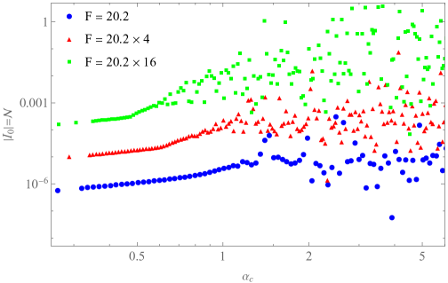
In Fig. 6, we plot the final zero-mode amplitude, $\lim_{T\rightarrow\infty}|I_{0}|\equiv\mathcal{N}$, with respect to $\alpha_{c}$ for different values of $F=F_{a}/H$. The data is obtained by numerically solving Eqs. (8), (9) and (61) for a large set of $c_{+}$ values using an Runge-Kutta solver (RK-solver) to a high numerical precision. From the plots, we observe that the amplitude of the zero-mode initially exhibits a continuous increase with respect to $\alpha_{c}$. However, as we explore in Appendix C, for $\alpha_{c}$ greater than a cutoff $\alpha_{{\rm Ch}}$ (where ${\rm Ch}$ stands for chaotic), the trajectory of the background fields $\phi_{\pm}$ becomes chaotic. Since the effective mass of the zero-mode is controlled by the dynamics of the background fields through the mass-squared matrix $\tilde{M}^{2}(\phi_{\pm})$, the zero-mode amplitude starts fluctuating chaotically. Consequently, in this region, $\mathcal{N}$ can be seen as a stochastic variable whose distribution depends on $c_{+}$ or $\alpha_{c}$. In such cases, the axionic fluctuation amplitudes have only a distributional prediction from the underlying Lagrangian parameters.

To understand the chaotic behavior, we note that the EoMs for the background fields given in Eqs. (8) and (9) represent a set of two quartically coupled oscillators. In the absence of dissipative and linear-force terms, the effective EoMs are described by a classical Yang-Mills-like potential ($V=x^{2}y^{2}/2$). It is well known in the literature (Carnegie_1984, ; Dahlqvist:1990zz, ; Marcinek:1994, ) that the classical Yang-Mills-like potential leads to chaotic motion, except for a very small set of initial conditions, due to a nonlinear mapping of the initial conditions through the nonlinear interactions. In the presence of dissipation term such as Hubble friction, the background fields must eventually settle to one of the local energy minima. Hence, the presence of dissipative Hubble term tends to make chaotic motion more orderly causing the system to converge to one of the equilibrium states. If the interaction and kinetic energy are considerable during the transition, we expect a transient chaotic phase until dissipation brings the system back to an ordered state.

Consequently, there is a critical threshold for the value of kinetic energy controlling parameter $\alpha_{c}$ below which chaos does not set in. In Appendix. C, we show examples of $\phi_{\pm}$ field trajectories for a chaotic case in Fig. 17 and further derive the condition for the onset of the transient chaotic motion. We show that to minimize transient chaos, the fast UV mode of the background fields, which is induced by $\xi$, should be negligible at the moment when the two fields cross each other. Assuming there are no crossings before transition, we obtain the condition

$$\left\langle\xi^{2}\right\rangle_{T_{{\rm 1}}}<2r^{2}F^{4}$$ (85)

to avoid transient chaos at the first crossing $T_{1}$ after transition time $T_{c}$, where $r\approx 0.2$ is an $O(0.1)$ number. In case of multiple crossings prior to the transition, the above condition must be applied to each crossing (including transition) where the UV modes are significant. Hence, in cases where the total energy during the crossings is large $\gtrsim O(F^{4})$, we expect the fields to behave chaotically.

Figure 7: Plot showing axionic isocurvature power spectra for two fiducial chaotic cases with a $0.5\%$ deviation in the values of $\Phi_{+}(0)$. Due to a large sensitivity of the field trajectories to the initial conditions, the resulting power spectrum amplitudes in the rising part of the spectrum and the initial few bumps can differ by orders of magnitude as seen in this example. For very short wavelength modes which exit the horizon when the field trajectories have either settled or track similar points in phase space, the power spectrum has similar amplitudes.

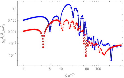
Due to the dependence of axion isocurvature fluctuation mode functions $I_{\pm}$ on the background fields via the mass-squared matrix $\tilde{M}^{2}$, significant variations in the trajectories of the background fields can lead to large changes in the amplitude of the final isocurvature modes. In Fig. 7, we present an example of the isocurvature spectrum obtained for a fiducial chaotic case, where we see a large deviation in the rising part of the spectrum and the first few bumps after the cutoff due to a small sub-percent deviation in the initial condition value of $\Phi_{+}(0)$. As highlighted in Fig. 7, the exponential sensitivity of the field trajectory on initial conditions can result in either a strong amplification or significant attenuation of the mode amplitude. Large amplification may occur when the background fields follow a trajectory that results in additional dips in the effective potential (leading to tachyonic masses), while attenuation can be caused by mode mixing corrections (large heavy mixing) or a slow roll of the background fields along a flat direction, leading to an exponential decay of the mode amplitude until the fields stabilize. We refer the interested reader to Chung:2021lfg  for further discussion on mode attenuation through an $m_{{\rm B}}^{2}$ parameter.

Another semi-quantitative way to see that the transient chaos of the background fields can lead to a chaotic isocurvature amplitude comes from the duality discussed earlier near Eq. (62). We know that there exists a time independent $\Xi_{1,2}=\Xi_{1,2}(c_{+},c_{-},F,\phi_{+}(0),\epsilon_{0})$ such that

$$\Xi_{1}I_{0}+\Xi_{1}^{*}I_{0}^{*}+\Xi_{2}I_{02}+\Xi_{2}^{*}I_{02}^{*}=\frac{I_{0}^{(\mathrm{dual})}}{f_{0}}=(\phi_{+},-\phi_{-})$$ (86)

where the right hand side is real and $I_{02}$ are zero modes independent of $I_{0}$ defined earlier that spans the solution space. When the right hand is a solution with different boundary conditions (e.g. for example change $\phi_{+}(0)$ without changing $c_{+}$), then the right hand side picks out a very different phase space trajectory because of the chaotic nature (as evidenced by Fig. 7). Let’s call this solution $\phi_{\pm}^{(2)}$:

$$\Xi_{1}^{(2)}I_{0}^{(2)}+\Xi_{1}^{(2)*}I_{0}^{(2)*}+\Xi_{2}^{(2)}I_{02}^{(2)}+\Xi_{2}^{(2)*}I_{02}^{(2)*}=(\phi_{+}^{(2)},-\phi_{-}^{(2)})$$ (87)

where $\{\Xi_{n}^{(2)},I_{0}^{(2)},I_{02}^{(2)}\}$ constitute a new set analogous to Eq. (86). Because $I_{0}\not\propto I_{0}^{(\mathrm{dual})}$ satisfies a different differential equation than $\phi_{\pm}$ and different boundary conditions, the new $\phi_{\pm}^{(2)}$ solution requires $\Xi_{n}^{(2)}$ that is drastically different than the original $\Xi_{n}$ (exponentially sensitive to the change in the initial conditions $\phi_{\pm}(0)$) to functionally match the different right hand side phase space trajectory.

Now, let’s see how this drastic change in $\Xi_{n}$ changes the coefficient $\mathcal{N}$ in Eq. (73) which characterize the amplitude at $T_{\infty}$ as

$$I_{0}(T_{\infty})\approx\mathcal{N}e^{i\theta}\psi_{0}$$ (88)

after the background fields have settled to their minima. Note that Eq. (88) only applies to situations in which the zero-mode matching of the mode function at the horizon exit can be identified with a single mode $I_{0}$ without mixing $I_{02}$. In such situations, substituting Eq. (88) into Eq. (86) evaluated at $T_{\infty}$, we see

$$\mathcal{N}\left(\Xi_{1}e^{i\theta}+\Xi_{1}^{*}e^{-i\theta}\right)\psi_{0}+\Xi_{2}I_{02}+\Xi_{2}^{*}I_{02}^{*}=(\phi_{+}(T_{\infty}),-\phi_{-}(T_{\infty}))$$ (89)

where at $T_{\infty}$, the $\phi_{\pm}$ goes to an attractor (i.e. the global minimum) despite the different initial conditions. However, as we have said above, since with different $\phi_{\pm}$ initial conditions $\Xi_{n}$ now has changed drastically say to $\Xi_{n}^{(2)}$, the other terms change ($\mathcal{N}\rightarrow\mathcal{N}^{(2)}$, $\theta\rightarrow\theta^{(2)}$) drastically to match the attractor of the right hand side: i.e.

$$\mathcal{N}^{(2)}\left(\Xi_{1}^{(2)}e^{i\theta^{(2)}}+\Xi_{1}^{(2)*}e^{-i\theta^{(2)}}\right)+\left(\Xi_{2}^{(2)}I_{02}^{(2)}+\Xi_{2}^{(2)*}I_{02}^{(2)*}\right)\cdot\psi_{0}$$

$$=\mathcal{N}\left(\Xi_{1}e^{i\theta}+\Xi_{1}^{*}e^{-i\theta}\right)+\left(\Xi_{2}I_{02}+\Xi_{2}^{*}I_{02}^{*}\right)\cdot\psi_{0}$$ (90)

where $\mathcal{N}\rightarrow\mathcal{N}^{(2)}$ change is chaotic with different initial conditions for $\phi_{\pm}$. Although one may naively not expect the parameter changes (such as $c_{+}$ changes) have much to do with the initial condition changes that translate to chaotically different phase space trajectories of $(\phi_{+},\phi_{-})$, small $c_{+}$ changes do map to different initial phase space points for $(\phi_{+},\phi_{-})$ through Eq. (15) when the nonlinear forces (governed by $\xi\phi_{-}$ of Eq. (24)) start to dominate say at time $T_{1}$ (with the linear force region initial conditions fixed).

On the other hand, different $K$ values do not control $(\phi_{+},\phi_{-})$ and will therefore not change their phase space trajectory. That is why the $\Delta_{s}^{2}$ has a $K$ spectral dependence that is still smooth (unlike the chaotic jumps in the overall normalization $\mathcal{N}$ as a function of $c_{+}$) in the $K$ region for which $\mathcal{T}_{K}<T_{c}$. When $\mathcal{T}_{K}$ is in the intermediate time region defined to be when the $\phi_{\pm}$ undergoes oscillations, the isocurvature amplitude oscillations as a function of $K$ can be complicated since the matching condition analogous to Eq. (66) but with a strongly oscillating function of time on the left hand side produces an oscillatory $c_{n}(K)$. That translates to different matching time $\mathcal{T}_{K}$ sampling the oscillations as a function of time and not strongly divergent phase space trajectories (chaos) due to effectively different initial conditions. In Secs. VI and VII we will present general fitting formulas for $\Delta_{s}^{2}(K)$ that can be used for practical fitting situations which would be sensitive to the first three bumps. In other words, the chaotic behavior of the map between the Lagrangian parameters and the amplitude does not present an obstacle for fitting $\Delta_{s}^{2}$ characteristic of this class of models as a function of $K$.

Of course, if the $K$ value is sufficiently large that $\mathcal{T}_{K}\gg T_{c}$, Eq. (66) is irrelevant and the amplitude is fixed by the usual massless mode nearly-exact solution in quasi-dS space:

$$I \approx-\frac{iH}{2k^{3/2}}\psi_{0}=\mathcal{N}\left(c_{1}(K)e^{i\theta}+c_{2}(K)e^{-i\theta}\right)\psi_{0}$$ (91)

which enters directly into Eq. (75). Even if $(\mathcal{N},\theta)$ changes drastically say with $c_{+}$ variation (discussed in Eq. (90)), $c_{1,2}(K)$ also changes drastically to compensate for the $(\mathcal{N},\theta)$ variation. There is no such compensating matching condition for $c_{n}(K)$ for smaller $K$s, as can be seen explicitly in Eq. (69) as they are fixed by a different function than the final nearly-exact solution.

In the next section, we provide analytic fitting functions for the zero-mode amplitude $\mathcal{N}$ as a function of $\alpha_{c},$ $F$, and $c_{-}$ for the non-chaotic cases where $\alpha_{c}<\alpha_{{\rm Ch}}$. For $c_{+}$ values where the background fields are chaotic, a closed-form analytic expression for the zero-mode function may not be feasible. For these cases, we propose a numerically motivated stochastic amplitude model with a log-normal distribution. Using the estimated value of $\mathcal{N}$ from these fits, one can approximate the amplitude of the axion isocurvature power spectrum from Eq. (75) for long-wavelength modes that exit the horizon prior to the transition of the background fields.

V Fitting functions for zero-mode amplitude

In Eq. (64), we provided the initial conditions for the zero-mode, $I_{0}$, at time $T_{0}\ll T_{c}$. Furthermore, in Sec. (IV.1), we noted that when $\phi_{+}\gg F$, the lightest mass eigenvalue is $m_{1}\approx c_{+}$, and during the time $T<T_{c}$ when the expansion parameter $\lambda=F^{2}/\phi_{+}^{2}<1$, the zero-mode solution can be approximated as

$$I_{0}(T)\approx e^{-\left(3/2+i\omega\right)T}\left[\begin{array}[]{c}1\\ -\lambda\end{array}\right].$$ (92)

The amplitude of $I_{0}$ during this time can be expressed as

$$\left|I_{0}(T)\right|\approx e^{-\frac{3}{2}T}.$$ (93)

As the background fields approach transition at $T_{c}$, we expect non-adiabatic behavior and heavy mode mixing due to a large interaction energy $\sim O(\xi^{2})\sim O(F^{4})\gg O(H^{2}F^{2})$. Hence, we define an amplification factor $\mathcal{Z}$ as

$$\mathcal{N}=e^{-\frac{3}{2}T_{c}}\mathcal{Z}$$ (94)

that captures the nontrivial amplification or attenuation of the zero-mode after the transition. In the succeeding subsections, we will provide an analytic fitting function and a distribution function for $\mathcal{Z}$ in the non-chaotic and chaotic cases respectively.

V.1 Non-chaotic: $\alpha_{c}<\alpha_{{\rm Ch}}$

For the non-chaotic cases where $\alpha_{c}<\alpha_{{\rm Ch}}$, the zero-mode amplitude increases monotonically with $\alpha_{c}$. From Fig. 6 we notice that the slope of the zero-mode amplitude in this parametric region changes at an intermediate value of $\alpha_{c}\approx\alpha_{2}$. As we have verified numerically and briefly explained in Chung:2021lfg , the change of slope corresponds to situations where large kinetic energy causes the background fields to cross at least once after the transition. Hence, for $c_{+}$ values where $\alpha_{c}<\alpha_{2}$, the background fields do not cross each other again after transition in the limit $c_{-}<O(1)$. At each crossing of the background fields, the system has a brief period of tachyonic mass dip in the effective mass of the lightest eigenmode. As a result, the mode function undergoes a brief period of amplification whenever the two background fields cross each other with a large relative kinetic energy. See Sec. 6 in Chung:2021lfg  for more details. Hence, for all $c_{+}$ values where the background fields cross again after transition, we expect additional amplification of the mode function. This explains the change in the slope of the zero-mode at $\alpha_{2}$.

Using a large set of numerical evaluations, we provide the following fitting functions for the zero-mode amplitude for non-chaotic cases for Lagrangian parameters $F$ and $c_{-}$ in the range, $F\equiv F_{a}/H\in[10,400]$ and $c_{-}\in[0.1,9/4]$:

$$\mathcal{Z} \approx f_{-}(c_{-})\times\begin{cases}c_{0}+c_{1}\sqrt{\alpha_{c}}&\alpha_{{\rm 1}}<\alpha_{c}<\alpha_{2}\\ 8.0+c_{2}\left(\alpha_{c}-\alpha_{{\rm Ch}}\right)&\alpha_{2}<\alpha_{c}<\alpha_{{\rm Ch}}\end{cases}$$ (95)

where the prefactor $f_{-}$ gives an approximate dependence of the zero-mode amplitude on $c_{-}$,

$$f_{-}(c_{-})\approx 0.26c_{-}^{0.5}+0.66c_{-}^{-0.29}\qquad 0.1<c_{-}<9/4.$$ (96)

For values of $c_{-}$ that lie outside the range $[0.1,9/4]$, we observe a multi-functional dependence of the mode amplitude on $F$ and $c_{\pm}$ as summarized in Tab. 1. We briefly discuss these cases in Appendix D. The fitting parameters are approximated using the following expressions:

$$c_{0} =2.99703-2.419\left(\frac{20.2}{F}\right)+2.5927\left(\frac{20.2}{F}\right)^{2}-1.2713\left(\frac{20.2}{F}\right)^{3},$$ (97)

$$c_{1} =0.07975+3.193\left(\frac{20.2}{F}\right)-4.2829\left(\frac{20.2}{F}\right)^{2}+2.2462\left(\frac{20.2}{F}\right)^{3},$$ (98)

$$c_{2} =\frac{9.127}{0.181+\left(20.2/F\right)},$$ (99)

and

$$\alpha_{{\rm Ch}}=1.0185\left(\frac{20.2}{F}\right)^{0.194}+0.4065\left(\frac{20.2}{F}\right)^{1.26}.$$ (100)

We set $\alpha_{2}$ as approximately,

$$\alpha_{2}=\alpha_{{\rm Ch}}-\frac{5.0}{c_{2}}$$ (101)

and

$$\alpha_{1}\approx 10^{-3}.$$ (102)

In Eq. (95), the specific form of $\mathcal{Z}$ for $\alpha_{c}<\alpha_{2}$ is motivated from Eq. (239) of Chung:2021lfg  where the authors derived analytic expressions for the mode amplitude in this parametric region. The lower cutoff is set at $\alpha_{1}\ll\alpha_{{\rm L}}\approx 0.2$ where $\alpha_{c}$ greater (lesser) than $\alpha_{{\rm L}}$ corresponds to resonant (non-resonant) underdamped fields. In Fig. 8, we compare our fitting function with the numerical results where we construct our fitting curves (solid lines) using Eq. (94) by taking the fitting function for $\mathcal{Z}$ from Eq. (95) and the analytical estimation of $T_{c}$ as given in Eq. (50). Over the range $\alpha_{{\rm L}}<\alpha_{c}<\alpha_{{\rm Ch}}$, the amplitude of zero-mode varies by $\sim O(10)$ which implies an $O(100)$ variation in the amplitude of the isocurvature power spectrum.

Figure 8: In this figure, we compare our fitting results with the numerical data for the zero-mode amplitude $\mathcal{N}$ as a function of $\alpha_{c}$, for three different values of $F=F_{a}/H$. The numerical data, plotted in solid markers, is the same as in Fig. 6, and we construct our fitting curve using Eq. (94) where we take the fitting function for $\mathcal{Z}$ from Eq. (95) and the analytical estimation of $T_{c}$ from Eq. (50).

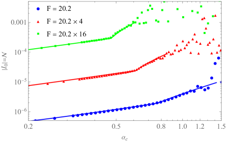
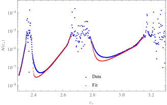
In Fig. 6, the $c_{+}$ values are restricted within the first branch ($j_{c}=1$). As we increase $c_{+}$, the parameter $\alpha_{c}$ makes a jump to the next branch $(j_{c}=2)$ and successive branches (See Fig. 3). In each branch, $c_{+}$ values that correspond to $\alpha\lesssim\alpha_{{\rm Ch}}$ belong to non-chaotic class of fields. Fig. 9 gives a plot of $\mathcal{N}$ for the first three branches ($j_{c}\leq 3$) for $F=20.2$ and shows the transition of mode amplitude within each branch from a smooth predictive behavior to random fluctuations due to chaotic background field dynamics.

Figure 9: In the plot on the left, we compare the zero-mode amplitude $\mathcal{N}$ obtained from the fitting formula in Eq. (95) (red square marker) with the numerical data (blue circular marker) for the first three branches highlighting the distinction between the non-chaotic and chaotic classes of fields based on the value of $\alpha_{c}$ as $c_{+}$ is varied from one branch to another. In each branch, we first estimate $\alpha_{c}$ and $T_{c}$ for the corresponding values of $c_{+}$ from the expressions given in Sec. III, and use the fitting function in Eq. (95) to obtain an approximation for the zero-mode amplitude in the non-chaotic region. For values of $c_{+}$ where $\alpha_{c}$ lies outside the fitting range of Eq. (95), the prediction is very sensitive to the values of $c_{+}$ such that only an approximate band of prediction can be realistically given. The mismatch between the fitting formula and the numerical results near the bottom of the troughs in the left plot occurs for non-resonant underdamped cases due to the smallness of the $\alpha_{c}$ value such that the separation between $T_{z,j_{c}}$ and $T_{c}$ is large ($\sim O(1)$). On the right, we plot $\alpha_{c}$ as a function of $c_{+}$ for the first 3 branches shown on the left. The dashed lines in this plot represents the lower and upper cutoffs at $\alpha_{{\rm L}}$ and $\alpha_{{\rm Ch}}$ respectively.

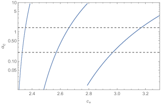
V.2 Noise model: $\alpha_{c}>\alpha_{{\rm Ch}}$

From Fig. 6 we infer that a closed form prediction of the final mode amplitude as a function of $\alpha_{c}$ is not feasible, unlike the fitting functions presented in Sec. V.1. For the fiducial case with $F=20.2$, the estimated cutoff $\alpha_{{\rm Ch}}\approx 1.4$ as given by Eq. (100). In Fig. 3, we have plotted the expected value of $\alpha_{c}$ against $\omega$ for $F=20.2$. Based on that figure, we can conclude that for $F=20.2$, values of $c_{+}\gtrsim 8.5$ will transition with $\alpha_{c}\gtrsim\alpha_{{\rm Ch}}$. In the limit, $F\gtrsim O(100)$, we estimate that massive underdamped fields with $c_{+}>O(5)$ do not have a stable predictive solution due to the chaotic behavior of the background fields. This represents a loss of predictability of the axionic model for massive fields. On the other hand, for any $\alpha_{c}>\alpha_{{\rm Ch}}$, there generically exists the phenomenological possibility of large amplitude enhancement without fine tuning of $\alpha_{c}$.

Figure 10: Histogram of the ${\rm\log}\left(\mathcal{Z}\right)$ over the noisy region for the fiducial choice of $F=20.2$ compared with an approximate normal distribution (solid blue curve).

To complete our analysis of the massive axionic underdamped fields, we show in Fig. 10 that the histogram of ${\rm\log}\left(\mathcal{Z}\right)$, for cases with $\alpha_{c}>\alpha_{{\rm Ch}}$, resembles a normal distribution. Therefore, we propose that for $\alpha_{c}>\alpha_{\mathrm{Ch}}$, the numerical data for $\mathcal{Z}$ can be approximated by a log-normal distribution given by the expression:

$${\rm pdf}\left({\rm log}\left(\mathcal{Z}\right)\right)=N\left(\mu,\sigma\right)$$ (103)

where the normal distribution $N\left(\mu,\sigma\right)$ has mean $\mu$ and variance $\sigma^{2}$. As seen in Fig. 6, the numerical data points in the chaotic region appear to be centered around a mean value. Using the log-normal distribution function, we estimate this mean amplification as

$$\left\langle\mathcal{Z}\right\rangle\approx e^{\mu+\frac{\sigma^{2}}{2}}$$ (104)

which would approximately correspond to the mode amplification from an average trajectory following the transition for the chaotic background fields. By fitting the numerical data, we find that the mean $\mu$ and variance $\sigma^{2}$ have the following approximate $F$ dependencies:

$$\mu(F) \approx 1.01+0.25\left(\frac{F}{20}\right)$$ (105)

$$\sigma(F) \approx 1.25+0.12\left(\frac{F}{20}\right).$$ (106)

Through the distribution function presented in this subsection and using the expression for the isocurvature power spectra for modes $k<k_{c}$ as outlined in Eq. (75), one can, at best, offer an approximate estimation for the average power within the blue region of the axion isocurvature spectrum. This applies specifically to massive underdamped fields that exhibit chaotic behavior owing to significant nonadiabaticity during their transition. This analysis is complementary to the fitting functions provided in subSec. V.1 for the non-chaotic dynamical system of background fields. However, these fits are limited to the blue-tilted region of the isocurvature power spectrum, and restricted to modes satisfying Eq. (70).

We do not have a simple, smooth prediction for the small-scale modes that lie within the oscillating part of the spectrum. This region of the power spectrum has a complex dependence on the underlying dynamical eigen-masses of the system of fields and as we shall see in the next section consists of a series of bumps (oscillations) with varying amplitudes. It was shown in Chung:2021lfg  that even the simplest cases require various analytical tools and the situation is compounded by the chaotic nature of the background fields implying that any fairly approximate estimation of the height of these bumps would require a complete numerical analysis of the mode equations as in Eq. (10).

In Chung:2021lfg , the authors presented an empirical piecewise mass-model motivated from a large set of analytical calculations including UV integration, nonlinear field redefinitions, and other techniques to approximate the shape and amplitude of the isocurvature power spectrum in the oscillating region. They found that for most non-chaotic cases, a generic non-minimal model with two negative square wells can be used to approximately map the power spectrum with variable bump heights in the small-scale region. In the next section, we will review the mass-model of Chung:2021lfg  and apply it to a few sample cases.

VI Empirical mass model

The mass-model presented in Chung:2021lfg  can be generalized into a Lagrangian independent numerical model. A Lagrangian-free model benefits from the variability and freedom of choice for the values of different parameters that can give rise to unique spectral shapes and amplitudes regardless of an underlying known or unknown action. The model will also allow us to fit isocurvature power spectra for cases that were beyond the scope of analytical methods presented in Chung:2021lfg . This is likely to be useful for fitting data and discovering isocurvature signatures. We begin by first introducing the mass-model and then use it to fit numerically obtained isocurvature power spectrum for the QCD axion toy-model presented in Sec. II.1.

Consider the following second-order linear differential equation for a scalar perturbation $y\left(K,T\right)$ in an expanding FRW spacetime:

$$\ddot{y}\left(K,T\right)+3\dot{y}\left(K,T\right)+\left(K^{2}e^{-2T}+m^{2}(T)\right)y\left(K,T\right)=0$$ (107)

where $m^{2}(T)$ encapsulates information regarding the form of the potential (mass and interactions) of the effective Lagrangian. Next, we define an effective mode-dependent mass-squared term

$$m_{{\rm eff}}^{2}\left(K,T\right)\equiv K^{2}e^{-2T}+m^{2}(T),$$ (108)

such that the differential equation takes the form

$$\ddot{y}\left(K,T\right)+3\dot{y}\left(K,T\right)+m_{{\rm eff}}^{2}\left(K,T\right)y\left(K,T\right)=0$$ (109)

and has the general solution

$$y\left(K,T\right)=c_{1}\psi_{1}\left(K,T\right)+c_{2}\psi_{2}\left(K,T\right).$$ (110)

To determine $\psi_{1,2}$ and solve the system of differential equations, we model $m_{{\rm eff}}^{2}$ through a piecewise discontinuous mass-model using the set of parameters

$$P_{{\rm set}}=\left\{V_{0},V_{1},V_{2},T_{1},T_{2},C_{m}\right\}+\left\{V_{i},T_{i},\Delta_{i}\right\}_{3\leq i\leq N}.$$ (111)

Thus, in each $K$-dependent time region $R_{(j)}$, the mass-model $m_{{\rm eff}(j)}^{2}$ takes the form

$$m_{{\rm eff}(j)}^{2}\left(K,T\right)\equiv A_{(j)}\left(K\right)e^{-n_{(j)}T}+c_{(j)}\quad\quad T\in R_{(j)}(K)$$ (112)

where $A_{(j)}(K)$ and $c_{(j)}$ are functions of the parameters in Eq. (111) and $n_{(j)}$ will take on a value from the set $\{3,5/2,2\}$ depending on the region $R_{(j)}$.The mass-model is based on the assumption that it is sufficient to follow the smooth (IR) behavior of the effective mass. Consequently, it incorporates a positive exponentially decaying term (derived from integrating out fast $O(F)$ UV oscillations of the lightest eigen-mass with a Hubble-driven decaying envelope) and a negative tachyonic mass-dip (associated with transient non-adiabatic effects) within each sub-region. In terms of the effective mass-squared $m_{{\rm eff}(j)}^{2}\left(K,T\right)$ in Eq. (112), the linearly independent solutions to the equation of motion presented in Eq. (109) in each region take the form

$$\psi_{1,2(j)}\left(K,T\right)=e^{-\frac{3}{2}T}J_{\pm\frac{\sqrt{9-4c_{(j)}}}{n_{(j)}}}\left(\frac{2}{n_{(j)}}A_{(j)}\left(K\right)e^{-\frac{n_{(j)}}{2}T}\right)$$ (113)

where $J_{\nu}$ is the cylindrical Bessel function. Thus, starting from $y\left(K,T_{0}\right)$, the final mode amplitude $y\left(K,T_{\infty}\right)$ is obtained by evaluating appropriate scattering matrices $S\left(K,R_{(j)}\right)$ in each piecewise region $R_{(j)}$ using the linearly independent functions given in Eq. (113) and the derived parameters $A_{(j)}(K)$, $n_{(j)}$, and $c_{(j)}$ that specify the $m_{{\rm eff}(j)}^{2}$ in each region.

VI.1 Mass-Model Implementation

Using the parameter set $P_{{\rm set}}$ presented in Eq. (111), we will now define the mass-model to fit the blue axion isocurvature power spectrum for the axion toy model presented in Chung:2021lfg . The motivation for the mass-model and its parameterization in terms of the Lagrangian variables were covered previously in Chung:2021lfg . We define the model $m_{{\rm eff}(j)}^{2}$ as

$$m_{{\rm eff}(j)}^{2}-K^{2}e^{-2T}=\begin{cases}V_{0}&0\leq T\leq T_{1}\\ -V_{1}&T_{1}\leq T\leq T_{2}\\ V_{2}e^{-3\left(T-T_{2}\right)}+\sum_{i=3}^{N}\left(-V_{i}\right){\rm sqw}\left(T,T_{i},\Delta_{i}\right)&T_{2}\leq T<T_{\infty}\end{cases}$$ (114)

where

$${\rm sqw}\left(T,T_{i},\Delta_{i}\right)=\begin{cases}1&T_{i}\leq T\leq T_{i}+\Delta_{i}\\ 0&{\rm otherwise}\end{cases}$$ (115)

and we set $T_{0}=0$. Similarly we choose $T_{\infty}$ long after the background fields have settled to their minima. The initial parameter $V_{0}$ models the mass-squared term induced for the lighter mass eigenmode (that tracks axion) as the $\phi_{+}$ field is rolling down along the flat direction and $\phi_{-}\ll\phi_{+}$. Negative mass-squared terms (dips) like $V_{1}$ and $V_{i}$ are due to the nonadiabatic effects induced during the crossing of the two fields, where the nonadiabaticity is controlled by the relative velocity of the fields as they cross. The exponential term $V_{2}$ signifies a positive (stabilizing) mass-squared term induced due to the high frequency $O(F)$ resonant oscillations of the two fields along the steeper direction in the overall potential.

Except for the exponentially decaying $V_{2}$ term, all of the remaining $V_{i}$ parameters act as $c_{(j)}$ within our model and they define a constant mass-squared term where it is either stabilizing (positive) or tachyonic (negative). For the region $\left[T_{2},T_{\infty}\right]$, we can write the effective mass-squared term as

$$m_{{\rm eff}(j)}^{2}(K,T)-c_{(j)}=K^{2}e^{-2T}+V_{2}e^{-3\left(T-T_{2}\right)}\quad T\in\left[T_{2},T_{\infty}\right]$$ (116)

Thus, the effective mass-squared is a sum of exponentials with different decay constants and amplitudes. However, by construction, we require that the value of decay constant $n_{(j)}$ within each piecewise region $R_{(j)}$ be constant. Therefore, to specify a single decay constant $n_{(j)}$ and an amplitude $A_{(j)}(K)$, we perform our evaluations by dividing the region $\left[T_{2},T_{\infty}\right]$ into two more regions $\left[T_{2},T_{K}\right]$ and $\left[T_{K},T_{\infty}\right]$ such that $m_{{\rm eff}(j)}^{2}\left(K,T\right)$ in Eq. (116) is now given by

$$m_{{\rm eff}(j)}^{2}\left(K,T\right)-c_{(j)}\equiv\begin{cases}B_{1}\left(K\right)e^{-3T}&T_{2}\leq T\leq T_{K}\\ B_{2}\left(K\right)e^{-2T}&T_{K}\leq T<T_{\infty}\end{cases}$$ (117)

where $T_{K}$ and $B_{1,2}$ are $k$-dependent boundary and amplitudes, respectively. These are not model parameters and are only required for internal calculations. We define $T_{K}$ as the time when

$$\left(K^{2}e^{-2T}-V_{2}e^{-3\left(T-T_{2}\right)}\right)_{T=T_{K}}=0,$$ (118)

therefore

$$T_{K}=T_{2}+\ln\left(\frac{V_{2}}{K^{2}e^{-2T_{2}}}\right).$$ (119)

With the above definitions, we now give the amplitudes $B_{1,2}(K)$ in each region as

$$B_{1}\left(K\right)=\frac{\int_{T_{2}}^{T_{K}}dT\,\left(K^{2}e^{-2T}+V_{2}e^{-3\left(T-T_{2}\right)}\right)}{\int_{T_{2}}^{T_{K}}dT\,e^{-3T}}=\left(V_{2}e^{3T_{2}}+\frac{3}{2}K^{2}\left(\frac{e^{T_{2}}+e^{T_{K}}}{1+2\cosh\left(T_{K}-T_{2}\right)}\right)\right)$$ (120)

and

$$B_{2}\left(K\right)=\frac{\int_{T_{K}}^{T_{\infty}}dT\,\left(K^{2}e^{-2T}+V_{2}e^{-3\left(T-T_{2}\right)}\right)}{\int_{T_{K}}^{T_{\infty}}dT\,e^{-2T}}=\left(K^{2}+\frac{2}{3}Ve^{3T_{2}}\left(\frac{1+2\cosh\left(T_{K}-T_{\infty}\right)}{e^{T_{\infty}}+e^{T_{K}}}\right)\right).$$ (121)

For long wavelengths, $K$ can be small enough such that $T_{K}$ is very large. Let us then consider a long wavelength mode, such that an additional $-V_{3}$ dip lies within the first section $\left[T_{2},T_{K}\right]$. In this case, we can divide the region $\left[T_{2},T_{K}\right]$ into 3 sub-regions as follows:

$$\left[T_{2},T_{K}\right]=\left[T_{2},T_{3}\right]\cup\left[T_{3},T_{3}+\Delta_{3}\right]\cup\left[T_{3}+\Delta_{3},T_{K}\right],$$ (122)

while the last region $\left[T_{K},T_{\infty}\right]$ remains unchanged. Similarly, for a sufficiently large $K$ mode (short wavelength) if the dip $-V_{3}$ lies within the region $\left[T_{K},T_{\infty}\right]$ we obtain 3 new sub-regions

$$\left[T_{K},T_{\infty}\right]=\left[T_{K},T_{3}\right]\cup\left[T_{3},T_{3}+\Delta_{3}\right]\cup\left[T_{3}+\Delta_{3},T_{\infty}\right].$$ (123)

VI.2 Scattering matrices

After all the regions/sub-regions have been determined, we evaluate the scattering matrices in each region $R_{(j)}$ using the linearly independent functions $\psi_{1,2(j)}$ from Eq. (113) and the derived parameters $A_{(j)}(K)$, $n_{(j)}$ and $c_{(j)}$. Since $m_{{\rm eff}(j)}^{2}$ has the same form in each region given by Eq. (112), the scattering matrix that we will provide below is generic and applicable in all regions.

For a set of $N$ piecewise regions $R_{(\{1,...,N\})}$, the final mode amplitude is given by the expression

$$Y(K,T_{N})=\prod_{j=1}^{N}S(K,R_{(j)})Y(K,T_{0})$$ (124)

where

$$Y(K,T)=\left[\begin{array}[]{c}y(K,T)\\ \partial_{T}y(K,T)\end{array}\right]$$ (125)

for mode function $y(K,T)$.

The scattering-propagator matrix $S(K,R_{(j)})\equiv S(K,T_{U(j)},T_{L(j)})$ for a region $R_{(j)}=\left[T_{L(j)},T_{U(j)}\right]$ where the indices $U,L$ indicate upper and lower bounds for the region, is

$$S(K,T_{U(j)},T_{L(j)}) =\left[\begin{array}[]{cc}\psi_{1(j)}&\psi_{2(j)}\\ \dot{\psi}_{1(j)}&\dot{\psi}_{2(j)}\end{array}\right]_{T=T_{U(j)}}\left[\begin{array}[]{cc}\psi_{1(j)}&\psi_{2(j)}\\ \dot{\psi}_{1(j)}&\dot{\psi}_{2(j)}\end{array}\right]_{T=T_{L(j)}}^{-1}$$ (130)

$$=\Psi_{(j)}\left(T_{U(j)}\right)\Psi_{(j)}^{-1}\left(T_{L(j)}\right)$$ (131)

where $\Psi_{(j)}^{-1}$ represents an inverse operation on matrix $\Psi_{(j)}$, and the two square matrices on the RHS are evaluated at $T_{L(j)}$ and $T_{U(j)}$ respectively. Using Eq. (113), the matrix $\Psi_{(j)}$ in the RHS of Eq. (130) is explicitly given as

$$\Psi_{(j)}\left(T\right)=\left[\begin{array}[]{cc}\psi_{1(j)}&\psi_{2(j)}\\ \dot{\psi}_{1(j)}&\dot{\psi}_{2(j)}\end{array}\right]_{T}\equiv e^{-\frac{3}{2}T}\left[\begin{array}[]{cc}J_{r}\left(z\right)&J_{-r}\left(z\right)\\ \left(-3/2J_{r}\left(z\right)+\partial_{T}J_{r}\left(z\right)\right)&\left(-3/2J_{-r}\left(z\right)+\partial_{T}J_{-r}\left(z\right)\right)\end{array}\right]$$ (132)

where $z=2A_{(j)}\left(K\right)\exp\left(-n_{(j)}T/2\right)/n_{(j)}$ and order $r=\sqrt{9-4c_{(j)}}/n_{(j)}$ with the parameters $A_{(j)}(K)$, $n_{(j)}$ and $c_{(j)}$ for a region $R_{(j)}$ as defined previously.

VI.3 Numerical Fitting

We will now present a few examples where we utilize the mass-model to fit axion isocurvature power spectra obtained by numerically solving the axion toy model in Eqs. (8), (9) and (10) for different Lagrangian parameters using an RK-solver. The fitted isocurvature power spectrum can be expressed as

$$\Delta_{S,{\rm fit}}^{2}(K,T_{\infty})=C_{m}K^{3}\left|Y(K,T_{\infty})\right|^{2}$$ (133)

where $C_{m}$ is a normalization parameter from the parameter set $P_{{\rm set}}$ of Eq. (111) and $Y(K,T_{\infty})$ is obtained from Eq. (124) using the scattering matrices by taking $T_{N}\rightarrow T_{\infty}$. In Eq. (124), we set the initial mode amplitude $Y(K,0)$ using the adiabatic boundary conditions of the BD vacuum.

Let us consider a minimal case where we restrict ourselves to $i=2$ in Eq. (111). This minimal model is sufficient to fit isocurvature power spectra for both over as well as underdamped cases where the background fields do not cross each other again after transition at $T_{c}$. This generically refers to all situations with $\alpha<\alpha_{2}$ where $\alpha_{2}$ is an $F$ dependent cutoff and given in Eq. (101). Hence, the minimal model consists of $V_{0}$, a single $-V_{1}$ dip at transition followed by an exponentially decaying $V_{2}$ term. The minimal mass-model consists of four piecewise regions $R_{\{1,..,4\}}$ as shown below

$$\left[T_{0},T_{\infty}\right] =R_{(1)}\cup R_{(2)}\cup R_{(3)}\cup R_{(4)}$$ (134)

$$=\left[T_{0},T_{1}\right]\cup\left[T_{1},T_{2}\right]\cup\left[T_{2},T_{K}\right]\cup\left[T_{K},T_{\infty}\right].$$ (135)

The final mode amplitude when evaluated using Eq. (124) can be expressed as

$$Y(K,T_{\infty})=S(K,R_{(4)})S(K,R_{(3)})S(K,R_{(2)})S(K,R_{(1)})Y(K,T_{0}).$$ (136)

where we set $Y(K,T_{0})$ to the BD initial conditions

$$Y(K,T_{0})=\left[\begin{array}[]{c}y\\ \partial_{T}y\end{array}\right]_{T=T_{0}=0}=\frac{e^{iK}}{\sqrt{K}}\left[\begin{array}[]{c}1\\ -iK-1\end{array}\right]\quad\forall K^{2}\gg V_{0}-2$$ (137)

where $T_{0}=0$ and we have dropped factors such as $2\left[a(0)\right]^{3/2}\sqrt{H}$ since we are presenting a fitting function. Additionally, the parameters $A_{(j)}(K)$, $n_{(j)}$ and $c_{(j)}$ for each of the four regions $R_{\{1,..,4\}}$ are set from

$$A_{(j)}(K) =\left\{K^{2},K^{2},B_{1}\left(K\right),B_{2}\left(K\right)\right\}$$ (138)

$$c_{(j)} =\left\{V_{0},-V_{1},0,0\right\}$$ (139)

$$n_{(j)} =\left\{2,2,3,2\right\}$$ (140)

where $B_{1,2}$ are given by Eqs. (120) and (121). As an example, consider region $R_{(3)}=\left[T_{2},T_{K}\right]$ with $A_{(3)}(K)=B_{1}(K)$, $n_{(3)}=3$ and $c_{(3)}=0$. We can then evaluate the $\Psi_{(3)}$ matrix at upper boundary $T_{K}$ as

$$\Psi_{(3)}\left(T_{K}\right)=e^{-\frac{3}{2}T_{K}}\left[\begin{array}[]{cc}J_{1}\left(z\right)&J_{-1}\left(z\right)\\ \left(-\frac{3}{2}J_{1}\left(z\right)+\partial_{T}J_{1}\left(z\right)\right)&\left(-\frac{3}{2}J_{-1}\left(z\right)+\partial_{T}J_{-1}\left(z\right)\right)\end{array}\right]$$ (141)

with

$$z=\frac{2}{3}B_{1}\left(K\right)e^{-\frac{3}{2}T_{K}}.$$ (142)

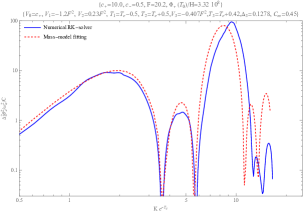
In Figs. 11 and 12, we present a few examples of axionic blue isocurvature power spectra fitted using the mass-model described above. In these examples, we have normalized the isocurvature spectra with respect to a constant

$$C=\frac{2r\left(1+r^{4}\right)}{\left(1+r^{2}\right)^{3}\pi^{2}F^{2}}$$ (143)

where $r=\sqrt{c_{+}/c_{-}}$ and set $T_{0}$ and $T_{\infty}$ to $0$ and $\sim 30$ respectively. In each case, the value of the axion Lagrangian variables and the fitted model parameters are shown in the title of the plots.

Figure 11: Fitting axionic blue isocurvature power spectra for examples where $\alpha<\alpha_{{\rm Ch}}$ using mass-model presented in Sec. VI. In each plot, solid (blue) curve represents the power spectrum obtained by solving Eqs. (8), (9) and (10) using an RK-solver while the dashed (red) curve is the fit from the mass-model. The plots in the top row are fitted using the minimal mass-model with $P_{{\rm set}}$ in Eq. (111) restricted to $N=2$, while the plots in the bottom row are examples of large resonant underdamped cases that are fitted using non-minimal mass-model with $N=3$ $(4)$ such that the model consists of additional $-V_{3}$ $(-V_{4})$ dips respectively.

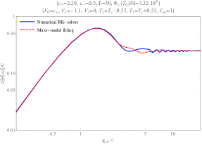
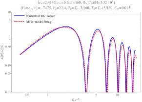
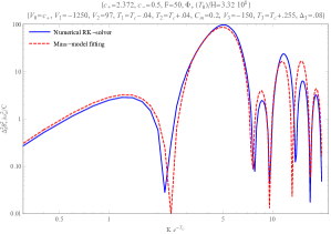
In Fig. 11 we restrict to examples where $\alpha_{c}<\alpha_{{\rm Ch}}$. The plots in the top row belong to the class of axion models where the background fields can be classified as non-resonant (resonant) oscillations of the fields post-transition where $\alpha_{c}<\alpha_{2}$. The non-resonant cases are defined by having $\alpha_{c}<\alpha_{{\rm L}}\sim 0.2$, where the shape of the isocurvature power spectrum for these cases bears resemblance to the overdamped case studied in Chung:2016wvv ; Chung:2017uzc . These are fitted using the minimal mass-model with $P_{{\rm set}}$ in Eq. (111) restricted to $N=2$ such that the model consists of a single $-V_{1}$ dip followed by an exponential $V_{2}$ potential. In the bottom row of Fig. 11 we fit the isocurvature spectra for cases with $\alpha_{c}>\alpha_{2}$. We observe that fitting these highly resonant underdamped instances, require non-minimal mass-model with $P_{{\rm set}}$ in Eq. (111) set to $N=3$ and $4$ respectively such that the model consists of additional $-V_{3}$ and $-V_{4}$ dips respectively. Finally, in Fig. 12 we present an example where we apply the mass-model to a chaotic case where we consider a large $c_{+}$ value such that $\alpha_{c}\gg\alpha_{{\rm Ch}}$. Through these examples, we conclude that the mass-model is a semi-quantitatively accurate representation of the axionic isocurvature power spectra with rich and complex spectral shapes and bumps.

Figure 12: Fitting axionic blue isocurvature power spectrum for a large $c_{+}$ case where $\alpha_{c}\gg\alpha_{{\rm Ch}}$ using mass-model presented in Sec. VI.

VII A sine function based fitting model

The mass model presented earlier provides a reasonable fit to the isocurvature spectrum over a broad range of scales. However, it involves intricate steps, a large number of fitting parameters, and can be time-consuming when searching for the best-fit values of the model parameters from numerical/observational data. From an observational perspective, the isocurvature spectrum can be divided into two regions: pre-cutoff ($k<k_{{\rm cut}}$) and post-cutoff scale ($k>k_{{\rm cut}}$) where we define $k_{{\rm cut}}$ as the location of the first bump in the power spectrum, which can be identified most simply as the first time when the slope of the power spectrum goes to zero followed by a decrease in the power. The pre-cutoff region is well described by a blue-tilt, while the post-cutoff region can undergo oscillations before settling to a massless plateau. In the context of detecting isocurvature modes and accurately fitting the signal, the initial bumps in the post-cutoff region are of utmost importance. To address this, we propose a simplified piecewise function that effectively captures and fits the isocurvature spectrum up to the first few bumps, or $k\lesssim O(5)k_{{\rm cut}}$: a $7$-parameter piecewise-model in terms of $x=2.08\,k/k_{{\rm cut}}$ written as

$$\Delta_{{\rm 2-fit}}^{2}\left(\left[c_{1-6},k_{{\rm cut}}\right],k\right)=\begin{cases}c_{1}\left|H_{i\sqrt{c_{2}-9/4}}^{1}(x)\right|^{2}x\left(j_{1}(x)\right)^{2},&x\lesssim x_{0}\\ \left(\sqrt{c_{1}\left|H_{i\sqrt{c_{2}-9/4}}^{1}(x_{0})\right|^{2}x_{0}\left(j_{1}(x_{0})\right)^{2}}\right.\\ \left.\phantom{\sqrt{\left|\right|^{2}}}+c_{3}\left(e^{-c_{4}x}\sin\left(c_{5}\left(x-c_{6}\right)\right)-e^{-c_{4}x_{0}}\sin\left(c_{5}\left(x_{0}-c_{6}\right)\right)\right)\right)^{2}&x_{0}\lesssim x\lesssim 10\end{cases}$$ (144)

where $j_{1}(x)$ is the spherical Bessel function of order $1$, and $H_{i\sqrt{c_{2}-9/4}}^{1}(x)$ is the Hankel function of order $i\sqrt{c_{2}-9/4}$. For underdamped cases, the first bump occurs at $x\approx 2.08$, and we find that choosing $x_{0}\approx 3$ yields a better matching and a lower $\chi^{2}$ when fitting the piecewise model to the numerical data for several examples. For the overdamped cases, which are characteristically defined by a blue-tilt of $1<n_{{\rm I}}<4$, and other scenarios with a smooth transition (without a bump) to the plateau, we find $x_{0}=0.4$ as a suitable choice. In Appendix E we briefly elaborate upon the motivation for this model construction, provide fitting parameters for the examples presented in Fig. 13 and give a fitting plot for a sample overdamped case.

Figure 13: In this figure we show plots where we fit the piecewise-model presented in Eq. (144) to the numerical data for four underdamped isocurvature power spectra examples. Starting from the top-left and moving clockwise, the examples presented in this figure can be further classified as non-resonant non-chaotic, resonant non-chaotic, resonant chaotic small $c_{+}$, and resonant chaotic large $c_{+}$ respectively.

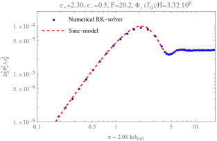
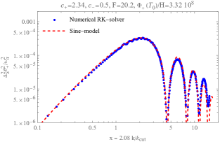
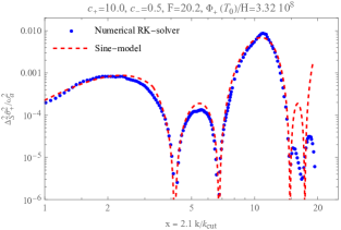
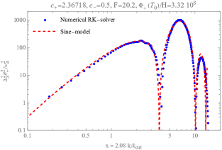
In Fig. 13, we fit the new piecewise sine-model to a few examples. In each case, the fiducial choice of Lagrangian parameters is given in the title of the plots. The fit model parameters are given in Appendix E. One can see from the $c_{+}=10.0$ case of Fig. 13 that the model does not fit the features of the spectrum for $k\gtrsim O(5)k_{{\rm cut}}$. The reason why the $k_{\mathrm{cut}}$ fixes the $k$ scale range over which the model is effective is because the number of oscillations in these isocurvature models has a fundamental oscillatory $k$-space period fixed by $k_{\mathrm{cut}}$, and one expects with a 7-parameter model to be able to fit at most 3 bump like features (counting around 2 parameters per bump). Of course, in principle, one may be able to add more parameters to fit more features for the higher $k$ values, but because near future surveys may be limited in the range of $k$-scale sensitivity, the 7-parameter model seems to strike a reasonable balance between economy and phenomenological detection coverage of the isocurvature perturbations in the near future. It is important to emphasize that the form of this fitting function was inspired by the generic solutions to the mass model that we discussed earlier.

VIII Conclusions

In this paper, we computed the axionic blue isocurvature perturbation power spectrum in the large radial field mass/kinetic energy limit for which there are multiple crossings of the radial field across the global minimum of the effective potential. This paper serves as a companion to the paper Chung:2021lfg . We have derived a mass model that can be used to compute the isocurvature spectrum based on the idea that the fast oscillating background fields have the net effect of a square well type of potential. Using this type of model, we have demonstrated that one can for example fit 7 bumps using 12 parameters. This type of model can be used for phenomenological fitting purposes if desired. To reduce the complexity of the possible future fitting efforts, we have also constructed a simpler 7-parameter sinusoid function based fitting function which fits at least 3 bumps, inspired by the results of the mass model. The new sine-model can be used to fit both underdamped as well as overdamped scenarios of the axionic model considered in this work, and may be applied model-independently to detect CDM isocurvature perturbations in scenarios where the axion mass makes a dynamical transition.

One interesting feature of the large kinetic energy cases considered in this paper was the appearance of exponential sensitivity of the isocurvature spectrum to Lagrangian parameters. This sensitivity arises because there is a large kinetic energy driven resonant phenomena that can exponentially boost or diminish amplitudes. Furthermore, the Lagrangian parametric variations which translate to changes in the initial conditions when the nonlinear forces temporarily dominate generically give rise to a background field phase space mixing that is characteristic of chaos. This means that although the spectrum generically has an oscillatory shape whose oscillatory $k$-period is fixed by the first collision time scale, the amplitude of the rising part of the spectrum and the first few oscillatory bumps determined by the background field phase space is not simply predictable as a function of the Lagrangian parameters controlling the kinetic energy of the radial field. That in turn implies that if we phenomenologically detect an oscillatory spectrum of the type considered in this paper, there will be a large theoretical uncertainty in mapping back to the underlying Lagrangian parameters. We quantify this uncertainty using a distribution function presented in Fig. 10.

In the construction of the rising part of the isocurvature spectrum, we have also noted that one can reduce the computation of the spectrum to solving the zero-mode amplitudes. In other words, we do not need to solve for the mode functions separately in the rising part of the spectrum as long as we have the background field solutions. This is owing to an accidental duality between the long wavelength mode equations and the background field equations present in the class of axion models considered in this paper. Using a set of numerical computations of zero-mode amplitudes, we have constructed a formula for the isocurvature spectrum in its rising part as a function of the underlying Lagrangian parameters in the non-chaotic region. We have also used the duality to explain the exponential parametric sensitivity of the spectrum in the chaotic region.

There are many interesting future directions related to this work. It would be interesting to carry out fits to data (or give forecasts for future experiments) using the fitting formulae presented in this work to look for signals of isocurvature perturbations. Most of the previous works on blue isocurvature spectrum have not dealt with the strongly oscillatory nature of the spectrum generic to the underdamped isocurvature scenarios. Moreover, even without the oscillations, most of the previous works have focused on simplified scenarios without a plateau cutting off the rising spectrum.

Given the large magnitude of the amplification of the high $k$ bumps (see e.g. Fig. 11), the non-Gaussianities generated by these isocurvature amplitudes may be significant and may have a spectral shape that is correlated with the power spectrum shape. This would be an interesting correlated non-Gaussianity study to pursue. One may also be able to use the large bump to generate seeds for unusually large clumped objects in the early universe such as primordial black holes Passaglia:2021jla . This enhancement of the power can also result in an overabundance of halos at high redshifts while converging to the halo mass function shape similar to that of $\Lambda$CDM at low redshifts Blinov:2021axd ; Tkachev:2023acf .

Appendix A $\phi_{\pm}$ Transient solutions

In Sec. III we demonstrated that when $\omega\gtrsim O(1)$, the background fields undergo a transition near a zero-crossing point at $T_{z,j}$ for $j\geq 2$. There we derived expressions to estimate the zero-crossing $T_{z,j_{c}}$ closest to the transition using a zeroth order approximate solution for the background fields. However, as the $\phi_{+}$ field moves closer to a zero-crossing $T_{z,j}$, significant deviations from the zeroth order solutions can occur due to a large kinetic energy $\sim O(\alpha^{2}F^{4})$ leading to transient effects.

In this Appendix, we will show that the non-adiabatic effects resulting from a zero-crossing at $T_{z,j}$ results in an $O\left(F/\alpha_{j}^{3/2}\right)$ increase in the effective mass of the $\phi_{+}$ field such that the location of the next zero-crossing at $T_{z,j+1}$ deviates from the expression provided in Eq. (27).

A.1 $\phi_{-,{\rm Tr}}$ solution

Since we assume that the background fields remain along the flat direction before they roll down to the minimum with $\phi_{+}(T_{0})\sim O(M_{P})$, the homogeneous solution of the $\phi_{-}$ field is negligible at $T_{0}$. However, as the $\phi_{+}$ field moves closer to its first zero-crossing $T_{z,j=1}$, a large kinetic energy $\sim O(\alpha^{2}F^{4})$ generates deviations in $\phi_{-}$ from the zeroth order solution. The homogeneous (transient) solution of the $\phi_{-}$ field can be obtained by solving the differential equation:

$$\ddot{\phi}_{-,{\rm Tr}}+3\dot{\phi}_{-,{\rm Tr}}+\left(c_{-}+\phi_{+}^{2}\right)\phi_{-,{\rm Tr}}\approx 0.$$ (145)

Thus, the transient component of $\phi_{-}$ oscillates rapidly with a high frequency $\sim O(\phi_{+})$. An approximate WKB solution to Eq. (145) can be written as

$$\phi_{-,{\rm Tr}}(T) \approx e^{-\frac{3}{2}\left(T-T_{*}\right)}\frac{A_{j}}{\sqrt{\left|\phi_{+}\right|}}\cos\left(\int_{T_{*}}^{T}dT\left|\phi_{+}\right|\right)\qquad T_{z,j}+\epsilon_{j}\lesssim T\lesssim T_{z,j+1}-\epsilon_{j+1}$$ (146)

where $T_{*}\sim T_{z,j}+\epsilon_{j}$ for $\epsilon_{j}\approx 1/\left(F\sqrt{\alpha_{j}}\right)$. To obtain an estimate for the amplitude $A_{j}$, we match the solution in Eq. (146) with the approximate solution given in Eq. (32) at $T_{z,j}+\epsilon_{j}$. This results in the following expression:

$$A_{j}\approx\frac{7}{4}\times\frac{F^{\frac{3}{2}}}{\alpha_{j}^{1/4}}.$$ (147)

After comparing with the numerical results, we modify the factor 7/4 in Eq. (147) to 2.3. This shift can be attributed to the inaccuracy of Eq. (32). For $T>T_{z,j}+O(1/F)$, the complete $\phi_{-}$ solution is given by the superposition of the forced and homogeneous solutions. In Fig. (14) we plot the background field for a fiducial case showing a comparison between the numerical solution and our approximate result in Eq. (146).

Figure 14: The plot illustrates a comparison between the analytic approximation (red, dashed line) of $\phi_{-,{\rm Tr}}$ as given by Eq. (146) and the corresponding numerical result (blue, solid line) for a specific example case where $T_{z,j=4}\approx 8$.

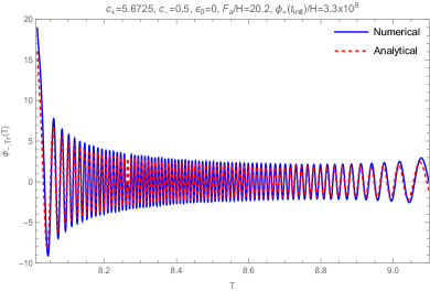
A.2 Transient mass-squared term

Due to the high frequency transient oscillations of $\phi_{-}$, the $\phi_{+}$ field inherits a positive mass contribution which leads to a decrease in the time period of oscillation. To see this explicitly we consider the EoM for $\phi_{+}$ and substitute $\phi_{-}\approx\phi_{-}^{(0)}+\phi_{-,{\rm Tr}}$ to analyze the effect of $\phi_{-,{\rm Tr}}$:

$$\ddot{\phi}_{+}+3\dot{\phi}_{+}+c_{+}\phi_{+}+\left(\left(\phi_{-}^{(0)}+\phi_{-,{\rm Tr}}\right)\phi_{+}-F^{2}\right)\left(\phi_{-}^{(0)}+\phi_{-,{\rm Tr}}\right)=0$$ (148)

which is equivalent to

$$\ddot{\phi}_{+}+3\dot{\phi}_{+}+\left(c_{+}+\phi_{-,{\rm Tr}}^{2}+2\phi_{-}^{(0)}\phi_{-,{\rm Tr}}\right)\phi_{+}-F^{2}\phi_{-,{\rm Tr}} =0.$$ (149)

By examining the aforementioned expression, it is evident that the $\phi_{+}$ field acquires a mass-squared term that oscillates rapidly with a high frequency. This oscillation is a result of the homogeneous oscillations of $\phi_{-}$. Through the UV integration procedure described in Appendix C of Chung:2021lfg , these high-frequency oscillations can be integrated out, leading to the determination of an effective mass-squared quantity composed of a residual IR term. More explicitly, we see that the dominant IR contribution is obtained through the UV integration of $\phi_{-,{\rm Tr}}^{2}$:

$$\phi_{-,{\rm Tr}}^{2}\underrightarrow{\leavevmode\nobreak\ \leavevmode\nobreak\ {\rm UV-Integration}\leavevmode\nobreak\ \leavevmode\nobreak\ }\frac{1}{2}\left(\frac{A_{j}e^{-\frac{3}{2}(T-T_{*})}}{\sqrt{\left|\phi_{+}\right|}}\right)^{2}.$$ (150)

After performing the UV integration, we obtain the reduced EoM for $\phi_{+}$ as follows:

$$\ddot{\phi}_{+}+3\dot{\phi}_{+}+c_{+}\phi_{+}+\frac{1}{2}A_{j}^{2}e^{-3(T-T_{*})}\approx 0\qquad T_{z,j}+\epsilon_{j}\lesssim T\lesssim T_{z,j+1}-\epsilon_{j+1}.$$ (151)

which has the following approximate solution :

$$\phi_{+}(x>\epsilon_{j}) \approx\frac{1}{8c_{+}\omega^{2}}\left(-4\omega^{2}A_{j}^{2}e^{-3x}+4\omega^{2}A_{j}^{2}e^{-3x/2}\cos(\omega x)-2\omega(3A_{j}^{2}-4c_{+}f)e^{-3x/2}\sin(\omega x)\right)$$ (152)

$$\approx\frac{\alpha_{j}F^{2}}{\omega}e^{-3x/2}\sin(\omega x)+\frac{A_{j}^{2}}{4c_{+}\omega}\left(-2\omega e^{-3x}+2\omega e^{-3x/2}\cos(\omega x)-3e^{-3x/2}\sin(\omega x)\right)$$ (153)

$$\approx\phi_{+}^{(0)}-\frac{A_{j}^{2}}{2c_{+}}\left(e^{-3x}-e^{-3x/2}\left(\cos(\omega x)-\frac{3}{2\omega}\sin(\omega x)\right)\right)$$ (154)

where $x=T-T_{z,j}$ , $f=\partial_{T}\phi_{+}(T_{z,j})\approx\alpha_{j}F^{2}$, and $\phi_{+}^{(0)}$ is the zeroth order perturbed solution given in Eq. (15).

In the limit $A_{j}\rightarrow 0$, we find $\phi_{+}\rightarrow\phi_{+}^{(0)}$. When the amplitude $A_{j}$ is finite and non-negligible, it results in a deviation from the background solution $\phi_{+}^{(0)}$. Consequently the next zero-crossing at $T_{z,j+1}$ occurs at

$$T_{z,j+1}-T_{z,j}=\frac{\pi}{\omega}-\Delta T\left(A_{j}\right)$$ (155)

where $\pi/\omega$ is the time period between two zero-crossings for the zeroth order perturbative solution $\phi_{+}^{(0)}$, and $\Delta T\left(A_{j}\right)$ is a function of $A_{j}$ which can be obtained by solving the transcendental equation corresponding to $\phi_{+}(T_{z,j+1}-T_{z,j})=0$ using Eq. (152).

Figure 15: In this figure we plot our analytic approximations, $\phi_{+}^{(0)}$ and $\phi_{+,{\rm An}}$, for the $\phi_{+}$ field using Eqs. (15) and (152) respectively. For comparison, we also plot the numerical results for $\phi_{\pm}$ fields. The fiducial values used for generating this plot are the same as the ones used in Fig. 14. A more accurate estimation of the amplitude $A_{j}$ of $\phi_{-,{\rm Tr}}$ will yield a better fit of $\phi_{+,{\rm An}}$ to the numerical results.

In Fig. 15 we plot $\phi_{+}$ using Eq. (152) and compare with the numerical solution for a fiducial case. Since $f\approx\alpha_{j}F^{2}$ and using Eq. (147) we can estimate the extent of the $A_{j}$-dependent deviation compared to the zeroth order solution:

$$\frac{\Delta\phi_{+}(A_{j})}{\phi_{+}^{(0)}}\approx O\left(\frac{F}{\sqrt{c_{+}}\alpha_{j}^{3/2}}\right).$$ (156)

Hence, the deviation from the $\phi_{+}^{(0)}$ solution is negligible for values of $\alpha_{j}\gtrsim O(F)$.

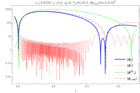
Appendix B Approximate estimation for $\theta$

In this Appendix, we give an approximate estimation of the phase, $\theta$, of the zero-mode solution, $I_{0}$. First, we note that the zero-mode solution, $I_{0}$, was initialized at $T_{0}$ as

$$I_{0}(T_{0})=e^{-\left(3/2+i\omega\right)T_{0}}e_{1}$$ (157)

from Eq. (63). For $\phi_{+}\gg F$, the lightest mass eigenvalue is $m_{1}\approx c_{+}$, and during the time $T<T_{c}$ when $\lambda=F^{2}/\phi_{+}^{2}<1$, the zero-mode solution can be approximated as

$$I_{0}(T)=e^{-\left(3/2+i\omega\right)T}\left[\begin{array}[]{c}1\\ -\lambda\end{array}\right].$$ (158)

The argument of $I_{0}$ during this time is

$$\arg\left(I_{0}\right)\approx-\omega T.$$ (159)

As shown in Fig. 1, at the transition, $T=T_{c}$, the background fields cross each other momentarily and subsequently settle to the minimum of the potential. Since the underdamped background fields can deviate significantly from the flat direction at $T\sim T_{c}$ and the lightest mass eigenvalue can undergo $O(F_{a}/H)$ oscillations post-transition. For $c_{-}<c_{+}$, the oscillations do not contribute a time-averaged mass, thereby freezing the phase angle $\arg\left(I_{0}\right)$ at the transition. For such cases, the final phase angle $\theta$ can be approximated as

$$\theta\approx-\omega T_{c}.$$ (160)

The transition time, $T_{c}$, can be estimated using Eq. (50).

Appendix C Chaos in blue axion system

In this Appendix, we will show that the axion toy model potential leads to a dynamical system that can result in chaotic trajectories due to quartic nonlinear interactions in the $\phi_{\pm}$ phase space. When infinitesimally separated field trajectories traverse regions of local instability, they may undergo divergent paths and can indicate the possible presence of a chaotic system. We begin this analysis by taking our nonlinear second order system of ordinary differential equations in Eqs. (8) and (9) and rewriting them as

$$\ddot{\phi}+3\dot{\phi}+M^{2}(\phi)\phi=0$$ (161)

where

$$M^{2}(\phi)=\left[\begin{array}[]{cc}c_{+}+\phi_{-}^{2}&-F^{2}\\ -F^{2}&c_{-}+\phi_{+}^{2}\end{array}\right]$$ (162)

and $\phi=(\phi_{+},\phi_{-})$. As shown in Fig. 6, the above system exhibits chaotic behavior for $\alpha_{c}>\alpha_{{\rm Ch}}$.

To connect with existing literature, consider the following simplified system of equations

$$\ddot{\phi}_{\pm}+\phi_{\mp}^{2}\phi_{\pm}=0$$ (163)

by removing the dissipative and mass terms from the EoM in Eq. (161). Note that the above system of equations is a special case of a quartic coupled oscillator system with the Lagrangian

$$L\left(t,x,y\right) =\frac{1}{2}\left(\dot{x}^{2}+\dot{y}^{2}\right)-\frac{a}{2}\left(x^{2}+y^{2}\right)$$

$$-\left[\frac{b}{4}\left(x^{4}+y^{4}\right)+\frac{1}{2}cx^{2}y^{2}\right]$$ (164)

obtained by taking $a=b=0$, and $c=1$. A detailed numerical study of the Lagrangian in Eq. (164) using the surface of section technique was performed in (Carnegie_1984, ) where the authors concluded that for potential $V=x^{2}y^{2}/2$ where $c=1$, the motion is completely chaotic. However, (Dahlqvist:1990zz, ) showed that there exists a tiny island (occupying $0.005\%$ of the total phase space) of stable periodic orbits, which was followed by a second set of stable orbit discovered in (Marcinek:1994, ) (occupying $4$ orders of magnitude smaller region than found in (Dahlqvist:1990zz, )). Intuitively, chaos occurs due to a nonlinear map between small changes in the initial conditions and the integrated effects of nonlinear forces.

C.1 Effect of dissipation

Consider the effect of adding the dissipative term and the negative mass squared term as

$$\ddot{\phi}_{\pm}+3\dot{\phi}_{\pm}+\left(\phi_{+}\phi_{-}-F^{2}\right)\phi_{\mp}=0$$ (165)

where the factor of $3$ is the dissipative Hubble term. With the variable changes

$$x_{1,2}=\phi_{\pm}/F$$ (166)

and

$$\tau=TF$$ (167)

our EoMs ($i=\{1,2\}$) reduce to

$$\ddot{x}_{i}(\tau)+\gamma\dot{x}_{i}(\tau)+\left(x_{1}(\tau)x_{2}(\tau)-1\right)x_{j\neq i}(\tau)=0$$ (168)

where the new dissipative constant is $\gamma=3/F.$ For our blue axion system, the ICs at transition, $T_{c}$, can be approximately given as

$$\phi_{+}(T_{c})/F=\phi_{-}(T_{c})/F\approx 1-0.2\alpha_{c}$$ (169)

and

$$\dot{\phi}_{+}/F^{2}\approx-\alpha_{c}\qquad\dot{\phi}_{-}/F^{2}\approx 0.48-0.09/\sqrt{\alpha_{c}}.$$ (170)

Clearly, we see that the blue axion system with $\gamma=0$ (no Hubble dissipation/friction) is always chaotic, since the incoming velocities of the two fields $\phi_{\pm}$ do not lie within the island of stability ((Dahlqvist:1990zz, )) required for a stable periodic solution.

A non-zero positive value of $\gamma$ leads to a constant dissipation within the system. In the presence of dissipation, a mechanical system gradually approaches one of its local energy minima. In the context of the blue axion system, the trajectories in the $\phi_{\pm}$ phase space are asymptotically approaching the points ($\phi_{\pm}=\phi_{\pm,\min},\dot{\phi}_{\pm}=0$) known as “point” attractors. These point attractors have dimension zero as they correspond to a stable equilibrium point in the phase space. Generally, the presence of dissipation tends to make chaotic motion into a more orderly behavior. When a system consists of quartically coupled oscillators and exhibits chaotic behavior, the introduction of dissipative forces corresponding to quadratic dissipation functions with diagonal elements ($\gamma\neq 0$, or $F\neq\infty$) causes the system to converge to a fixed point. If the dissipation is very small, the system can display long-lasting chaotic transients. Such transient chaos in dissipative systems is thus essentially a phenomenon that occurs when certain factors, such as the amplitude of the driving force being above a particular value or friction constant being below a threshold value.

For our blue axion system, the critical chaos-inducing nonlinear force is proportional to $\xi=\phi_{+}\phi_{-}-F^{2}$. Hence, if the average interaction and kinetic energy are substantial during the transition, we anticipate a temporary phase of chaos until dissipation restores order in the system. Thus, there must exist a threshold limit on the value of $\alpha_{c}$ below which chaos does not set in for more than a few $O(1/F)$ time-period.

Figure 16: Plot showing number of crossing (for $\tau>0$) as a function of parameter $\alpha_{c}$ for different values of dissipative constant $\gamma=3/F$.

Figure 17: In each frame, we plot trajectories of $\phi_{\pm}$ fields (thick curve) and a similar perturbed system (thin curve) with a $1\%$ deviation in the ICs. The plot on the left (right) correspond to case where $\alpha_{c}$ is lower (higher) than $\alpha_{{\rm Ch}}$. We find that tiny changes in the ICs can result in large deviations in the trajectories when $\alpha_{c}$ is larger than the threshold value $\alpha_{{\rm Ch}}$.

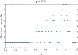
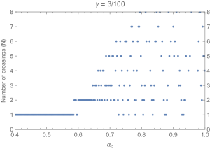
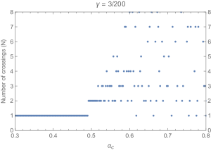
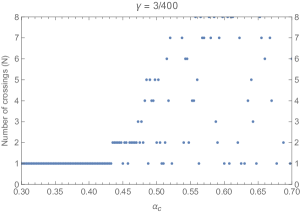
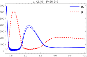
To illustrate the onset of chaos in the presence of dissipation, we solve the coupled oscillator system in Eq. (168) by initializing at $\tau=0$ with the initial conditions similar to that of the blue axionic system at transition. Hence, we set

$$x_{1}=x_{2}=1-0.2\alpha_{c},$$ (171)

$$\dot{x}_{1}=-\alpha_{c}\qquad\dot{x}_{2}=0.48-0.09/\sqrt{\alpha_{c}}$$ (172)

and plot the number of times $x_{1,2}$ cross each other for $\tau>0$ as a function of the parameter $\alpha_{c}$ for four different values of dissipative constant $\gamma=3/F$ in Fig. 16. In each scenario, we observe a phenomenon where the number of crossings, denoted as $N$, becomes random (unpredictable) once the parameter $\alpha_{c}$ becomes larger than a threshold value $\alpha_{{\rm Ch}}$. Across all cases, the onset of chaos seems to occur as $N$ becomes larger than $1$, indicating a significant kinetic energy level allowing the oscillators to cross more than once after $\tau=0$.

In Fig. (17) we graph the trajectory of $\phi_{\pm}$ fields for two sample $c_{+}$ values corresponding to $\alpha_{c}$ lower and higher than the threshold $\alpha_{{\rm Ch}}$ respectively. Within each frame, we also depict a “similar” perturbed $\phi_{\pm}$ system with a $1\%$ deviation in the ICs. We observe that as $\alpha_{c}$ surpasses the threshold value $\alpha_{{\rm Ch}}$, the field trajectories can be highly sensitive to the ICs due to the dominance of the nonlinear quartic interaction.

In a qualitative sense, the chaos tends to become important at the moment of the first crossing of the oscillators after $\tau=0$. This may be understood by noticing that as the average interaction energy exceeds a specific threshold, the subsequent motion (trajectory) following the crossings can exhibit extensive divergence due to rapid oscillations ($\gg O(\gamma)$) of the interaction term. To obtain a quantitative limit, we note that in the blue axion system, the interaction term $\xi$ induces a high frequency component, $\phi_{\pm,f}$, to the background field solution. Compared to the slow varying IR mode, the UV mode has a strength approximately given by the ratio $\xi/\Omega^{2}$ where $\Omega^{2}=\phi_{+}^{2}+\phi_{-}^{2}$. Based on our qualitative reasoning, we estimate that to initiate chaos, the UV mode should be important at the first crossing, $T_{1}$ (after transition). Hence we require for the lack of chaos the condition

$$\left.\frac{\xi}{\Omega^{2}}\right|_{T_{1}} <r\ll 1$$ (173)

where $r$ is an $O(0.1)$ number. Since $\Omega^{2}=2F^{2}$ at $T_{1}$, we obtain the condition

$$\left.\xi^{2}\right|_{T_{1}}\ll r^{2}4F^{4}.$$ (174)

The time average of this quantity over $1/F$ time scale yields

$$\left\langle\xi^{2}\right\rangle_{T_{1}}\ll 2r^{2}F^{4}.$$ (175)

Numerical analysis reveals that the coupled oscillator system undergoes transient chaotic motion when the average interaction energy $\left\langle\left(x_{1}x_{2}-1\right)^{2}\right\rangle\approx(1/2)E(0)\exp(-\gamma\tau)$ at the point of first crossing $(\tau_{1}>0)$ is approximately $>0.1$. In the context of the blue axion system, this condition for the transient chaotic behavior can be expressed as

$$\left\langle\xi^{2}\right\rangle_{T_{1}}\approx(1/2)E(T_{c})\exp(-3(T_{1}-T_{c})))\gtrsim\left(0.1\right)F^{4}$$ (176)

where $E(T_{c})$ is the total energy at transition. This $0.1$ number was numerically inferred with $c_{+}/F^{2}\ll 0.1$ and can be interpreted as the number related to the Hubble expansion rate and does not reflect the $c_{+}$ parametric dependence. Presumably, the right-hand side of Eq. (176) has contributions that are $c_{+}F^{2}$ which would become important when $c_{+}/F^{2}$ become comparable to $0.1$. These numerical findings align with the condition described in Eq. (175), by setting the $O(0.1)$ parameter $r\approx 0.2$. Hence, while the total energy at the transition is approximately $O(\alpha_{c}^{2}F^{4})$, the Hubble friction must cause sufficient damping to achieve a stable trajectory for the background fields. Since $T_{1}$ is a function of $F$ and $\alpha_{c}$, we get the following condition for stable trajectories

$$T_{1}(F,\alpha_{c})\gtrsim T_{c}(F,\alpha_{c})+\frac{1}{3}\ln\left(\frac{f(\alpha_{c})}{0.2}\right)$$ (177)

where the function $f(\alpha_{c})=E(T_{c})/F^{4}$ and can be approximately given as

$$f(\alpha_{c})\approx\alpha_{c}^{2}+(0.48-0.09/\sqrt{\alpha_{c}})^{2}$$ (178)

where we have neglected mass contributions of order $F^{2}$.

Appendix D Exploring $c_{-}$ dependence

$c_{-}$	$\alpha_{c}(c_{+})<\alpha_{2}$	$\alpha_{2}<\alpha_{c}(c_{+})\lesssim\alpha_{{\rm Ch}}$	$\alpha_{c}(c_{+})>\alpha_{{\rm Ch}}$
$<O(0.1)$	exponential increase/decay	exponential increase/decay	Chaotic
$<9/4$	$(1/c_{-})^{O(0.25)}$	$(1/c_{-})^{O(0.25)}$	Chaotic
$F^{2}\gg c_{-}>9/4$	smooth increase	Oscillating function of $c_{-}$	Chaotic

Table 1: Table summarizing the approximate dependence of the zero-mode amplitude on the Lagrangian mass parameters $c_{\pm}$, where we have explicitly considered the $c_{+}$ dependence of the spectrum using the parameter $\alpha$. The boundaries $\alpha_{2}$ and $\alpha_{{\rm Ch}}$ are approximately independent of $c_{-}$ for $c_{-}\ll F^{2}$. For example, Eq. (100) still governs $\alpha_{{\rm Ch}}$ in the range of $c_{-}$ here.

Figure 18: Plot showing the $c_{-}$ dependence of the zero-mode amplitude $\mathcal{N}$ for four fiducial instances. The black-dashed line is our fitting curve as given in Eq. (187). For each distinct value of $F$, the corresponding $c_{+}$ values belong to $\alpha_{c}<\alpha_{2}$ and $\alpha_{2}<\alpha_{c}\lesssim\alpha_{{\rm Ch}}$ cases respectively.

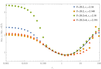
Post transition, $|\phi_{-}|$ begins to increase due to a positive velocity of $O(F^{2})$ and becomes dominant compared to a decreasing $|\phi_{+}|$. During this time, the UV integrated EoM for the IR component of the dominant $|\phi_{-}|$ field can be given as

$$\partial_{T}^{2}\phi_{-s}+3\partial_{T}\phi_{-s}+\left(c_{-}+\frac{A^{2}}{2\bar{\Omega}^{2}}e^{-3(T-T_{2})}\right)\phi_{-s}+\sqrt{c_{+}c_{-}}\phi_{+s}\approx 0$$ (179)

where the subscript $s$ denotes IR (slow) component, $T_{2}\approx T_{c}+O(1/F/\sqrt{\alpha_{c}})$ , $A/\bar{\Omega}$ is the effective amplitude obtained through the UV integration of the nonlinear interaction term $\propto\xi$ as explained in Appendix E of Chung:2021lfg . During this time, $\phi_{+s}\approx F^{2}/\phi_{-s}$. In the limit $\phi_{-s}>\phi_{+s}$, the general solution to the above ordinary differential equation is

$$\phi_{-s}(T)=e^{-\frac{3}{2}(T-T_{2})}\left[c_{1}J_{n}\left(\frac{2}{3}Ae^{-\frac{3}{2}(T-T_{2})}\right)+c_{2}J_{-n}\left(\frac{2}{3}Ae^{-\frac{3}{2}(T-T_{2})}\right)\right]$$ (180)

where

$$n=\sqrt{1-4c_{-}/9}$$ (181)

and the coefficients $c_{1,2}$ are obtained by matching with the incoming solution at $T_{2}$.

At a later time in the evolution of the background fields when the $A/\bar{\Omega}$ term in Eq. (179) can be neglected (due to exponential decay), the solution in Eq. (180) reduces to

$$\phi_{-s}(T)=e^{-\frac{3}{2}(T-T_{2})}\left[c_{1}e^{\frac{3}{2}n(T-T_{2})}+c_{2}e^{-\frac{3}{2}n(T-T_{2})}\right].$$ (182)

For $c_{-}<9/4$, the exponent $n$ is real, and it was shown in Chung:2021lfg that the evolution of the background fields towards the minimum of the potential is governed by an $O(c_{-}/3)$ exponent. Hence, we can write

$$\lim_{T\rightarrow T_{\infty}}\phi_{-s}(T)\approx\phi_{-\min}\left(1\pm e^{-\lambda(T-T_{\infty})}\right)$$ (183)

where $\lambda\approx O(c_{-}/3)$. The $+(-)$ sign indicates the direction of the field’s movement where $\phi_{-}(T)$ is greater (lesser) than $\phi_{-\min}$ as $T\rightarrow T_{\infty}$.

Due to the duality between the zero-mode and the background fields (see Eq. (62)), the evolution of the zero-mode is closely related to that of the background fields, resulting in an increase/decrease of the zero-mode amplitude. Because the rolling of the $\phi_{-}$ continues until the $\phi_{-}$ field reaches its minimum at $\phi_{-\min}$, the zero mode amplitude can be written as

$$I_{0}(T_{\infty})\approx I_{0}(T\gg T_{2})\frac{\phi_{-\min}}{\phi_{-}(T)}.$$ (184)

Hence, for $c_{-}<9/4$ the leading $c_{-}$ dependence of the zero-mode amplitude is

$$\mathcal{N}\propto\phi_{-\min}\propto\left(\frac{1}{c_{-}}\right)^{1/4}$$ (185)

because $\phi_{-\min}\approx F\left(c_{+}/c_{-}\right)^{1/4}$. By matching with the numerical data, we obtain the following fitting function for the zero-mode amplitude

$$\mathcal{N}\left(O(0.1)<c_{-}<9/4,c_{+},F\right)\equiv f_{-}(c_{-})\mathcal{N}\left(c_{-}=0.5,c_{+},F\right)$$ (186)

where

$$f_{-}(c_{-})\approx 0.26c_{-}^{0.5}+0.66c_{-}^{-0.29}.$$ (187)

Thus, the zero-mode amplitude increases as an inverse power of decreasing $c_{-}$ for $c_{-}<O(1)$. Interestingly, if $c_{-}\sim O(0.01)$ the exponential slow roll after transition can be extremely gradual, causing the fields to not fully settle at the minima of the potential by the end of inflation. This slow roll of the fields is analogous to inflationary slow roll situations, and in the current axion model this parametric region is $c_{+}\lesssim O(0.1)$. Consequently, the mode amplitude at $T_{{\rm end}}$ (number of e-folds to the end of inflation) appears to be either amplified or attenuated due to the insufficient number of e-folds for the background fields to settle down. This amplification (attenuation) of the mode amplitude occurs when $\phi_{-}(T_{{\rm end}})$ is greater (smaller) than $\phi_{-\min}$, and the parametric $c_{-}$ dependence is given approximately by $\sim\exp\left(O(c_{-})(T_{\infty}-T_{{\rm end}})\right)$ where $T_{\infty}$ is the hypothetical number of e-folds required for the background fields to settle to the minima. The value of $T_{\infty}$ is approximately dependent upon the maximum amplitude $\phi_{-\max}$ which, in turn, is controlled by the Lagrangian parameters $c_{\pm}$ and $F$. This subtle yet interesting dynamics for extremely small $c_{-}$ values was not pointed out in Chung:2021lfg .

For $c_{-}>9/4$, we first consider the case where the $A^{2}$ term in Eq. (179) is negligible, applicable to scenarios where $\alpha_{c}<\alpha_{2}$. In these cases, the exponent $n$ in Eq. (180) is imaginary and the solution for $\phi_{-s}$ becomes oscillatory, leading to subsequent crossings of the two fields after the transition. At each crossing, the lightest eigen-mass briefly becomes tachyonic (due to a short, significant excursion of $-\partial_{T}e_{1}.\partial_{T}e_{1}$) resulting in an amplification of the zero-mode. The amplitude of the tachyonic dip depends upon the magnitude of eigenvector rotation $\propto-\partial_{T}e_{1}.\partial_{T}e_{1}$ which decays as $\sim\exp\left(-3\left(T-T_{c}\right)\right)$ where $T_{c}$ should be distinguished from crossing times other than the first. Hence, as $c_{-}$ increases beyond $9/4$, because the background fields oscillate with a short time-scale $\propto 1/\sqrt{c_{-}}$, the tachyonic amplitude is larger at each crossing, consequently making the final mode amplitude larger where the steepness of the rise in amplitude (which is characterized by the coefficient $c_{1}$ in Eq. (95)) increases as function of $c_{-}$.

When $\alpha_{2}<\alpha_{c}<\alpha_{{\rm Ch}}$, the $A^{2}$ term in Eq. (179) is significant, and the fields must cross again after the transition. Close to the crossing, the incoming velocity of the sub-dominant field $\phi_{+}$ has a significant contribution from the fast UV oscillations, $\phi_{-f}\sim A/\Omega^{2}\sin(\int_{0}^{T-T_{2}}\Omega(x)dx)\phi_{-s}$ where $\Omega=\sqrt{\phi_{+s}^{2}+\phi_{-s}^{2}}\sim O(F)$ and $A\sim O(\alpha_{c}F^{2})$. A finite value of $c_{-}$ leads to a marginal increase in the frequency of $\Omega\sim\phi_{-s}$ causing the fields to cross earlier. As a result, the phase $\theta=\int_{0}^{T-T_{2}}\Omega(x)dx$ of $\phi_{+f}$ at the crossing reduces. For $c_{-}$ values larger than a threshold, the change in the phase angle, $\Delta\theta$, can be order $1$, leading to the oscillatory pattern in the final zero-mode amplitude as a function of $c_{-}$ as observed in Fig. 18 for $c_{+}=2.348$ and $2.391$. Up to leading order in $c_{-}$, we find semi-analytically that we can approximate $\Delta\theta\approx c_{-}\left(0.25+0.2\left(F/20.2\right)\right)$ which implies an almost $F$ independent lower bound of $c_{-}\sim O(2)$ for the oscillations to be prominent.

Appendix E Fitted sine-model parameters

The sine model presented in Sec. VII can be most generally written as

$$\Delta_{{\rm 2-fit}}^{2}\left(\left[c_{1,..,8},k_{{\rm cut}}\right],k\right)=\begin{cases}c_{1}\left|H_{i\sqrt{c_{2}-9/4}}^{1}(kc_{3})\right|^{2}\left(kc_{3}\right)\left(j_{1}(kc_{3})\right)^{2}&k\lesssim k_{{\rm cut}}\\ \left(c_{4}+c_{5}e^{-c_{6}k}\sin\left(c_{7}\left(k-c_{8}\right)\right)\right)^{2}&k_{{\rm cut}}\lesssim k<O(5)k_{{\rm cut}}\end{cases}$$ (188)

where $j_{1}(x)$ is the spherical Bessel function of order $1$, and $H_{i\sqrt{c_{2}-9/4}}^{1}(x)$ is the Hankel function of order $i\sqrt{c_{2}-9/4}$. The functional form of the fitting function in the blue region ($k<k_{{\rm cut}}$) is jointly motivated from the analysis presented in Sec. IV.1 and from the results of Chung:2021lfg . Readily one can identify that $c_{2}>9/4$ for underdamped cases and $<9/4$ for overdamped fields. The first bump in the isocurvature spectrum (for critical and underdamped cases) lies at the location $k_{{\rm cut}}$. From Eq. (188), we observe that the first bump of the fitting model is primarily determined by the function, $j_{1}(kc_{3})$. For the spherical Bessel function, $j_{1}(x)$, the first bump occurs at $x\approx 2.08$. Consequently, we deduce that $k_{{\rm cut}}c_{3}\approx 2.08$, and therefore, we can eliminate $c_{3}$ as $c_{3}\approx 2.08/k_{{\rm cut}}$.

We model the post-cutoff region in Eq. (188) using a sine function with an amplitude that exponentially depends on the mode $k$. During the fitting procedure, we choose a scale $k_{0}$ as the boundary where we match the two piecewise functions. The matching allows us to eliminate another model parameter. Hence, consider the following expression where we match the amplitude of the two piecewise functions in Eq. (188) at an arbitrary scale $k_{0}$:

$$c_{1}\left|H_{i\sqrt{c_{2}-9/4}}^{1}(k_{0}c_{3})\right|^{2}\left(k_{0}c_{3}\right)\left(j_{1}(k_{0}c_{3})\right)^{2} =\left(c_{4}+c_{5}e^{-c_{6}k_{0}}\sin\left(c_{7}\left(k_{0}-c_{8}\right)\right)\right)^{2}.$$ (189)

Using the above expression we eliminate $c_{4}$ as

$$c_{4}=\sqrt{c_{1}\left|H_{i\sqrt{c_{2}-9/4}}^{1}(k_{0}c_{3})\right|^{2}\left(k_{0}c_{3}\right)\left(j_{1}(k_{0}c_{3})\right)^{2}}-c_{5}e^{-c_{6}k_{0}}\sin\left(c_{7}\left(k_{0}-c_{8}\right)\right).$$ (190)

Substituting the above expression for $c_{4}$ into Eq. (188) and redefining the remaining parameters yields the form of the model presented in Eq. (144).

Figure 19: In this figure we present plot obtained from fitting the sine-model to a fiducial overdamped scenario.

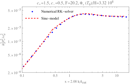
Fig. 19 displays an example where we fit the sine-model to an overdamped isocurvature power spectrum covered extensively in Chung:2016wvv . The plots in Figs. 13 and 19 illustrate that the sine-model can be extended to analyze and fit cases beyond the underdamped scenario of the axion toy model considered in this work. It may also be applicable to other Lagrangian models that produce similar shapes of the isocurvature power spectra.

In the rest of this appendix, we provide the best-fit values of the model parameters obtained by fitting the piecewise model in Eq. (144) to the numerical isocurvature power spectra examples shown in Sec. .VII. In each case mentioned below, we use $x=2.08k/k_{{\rm cut}}$. As discussed in Sec. VII, for the overdamped (underdamped) cases, we find $x_{0}\approx 0.4$ ($3.0$) is a suitable choice for fitting:

1. $c_{+}=2.30$, $c_{-}=0.5$, $F=20.2$, $\epsilon_{0}=0$, $\phi(T_{0})=3.32\times 10^{8}$:

   $$c_{1}=0.000361,\,c_{2}=2.3226,\,c_{3}=-0.03957,\,c_{4}=0.88344,\,c_{5}=1.40334,\,c_{6}=3.97287$$ (191)

   and $k_{{\rm cut}}/\left(a_{i}H\right)\approx 2.0\times 10^{5}$.

2. $c_{+}=2.34$, $c_{-}=0.5$, $F=20.2$, $\epsilon_{0}=0$, $\phi(T_{0})=3.32\times 10^{8}$:

   $$c_{1}=0.000816,\,c_{2}=2.40618,\,c_{3}=0.02156,\,c_{4}=0.13236,\,c_{5}=0.89631,\,c_{6}=0.97835$$ (192)

   and $k_{{\rm cut}}/\left(a_{i}H\right)\approx 3.2\times 10^{4}$.

3. $c_{+}=2.36718$, $c_{-}=0.5$, $F=20.2$, $\epsilon_{0}=0$, $\phi(T_{0})=3.32\times 10^{8}$:

   $$c_{1}=307.29,\,c_{2}=2.50251,\,c_{3}=33.571\,c_{4}=0.06304,\,c_{5}=0.61706,\,c_{6}=-0.82489$$ (193)

   and $k_{{\rm cut}}/\left(a_{i}H\right)\approx 1.7\times 10^{4}$.

4. $c_{+}=10.0$, $c_{-}=0.5$, $F=20.2$, $\epsilon_{0}=0$, $\phi(T_{0})=3.32\times 10^{8}$:

   $$c_{1}=1.8431\times 10^{-6},\,c_{2}=9.98452,\,c_{3}=0.04836,\,c_{4}=0.000067,\,c_{5}=0.59356,\,c_{6}=-2.4721$$ (194)

   and $k_{{\rm cut}}/\left(a_{i}H\right)\approx 1.6\times 10^{4}$.

5. $c_{+}=1.5$, $c_{-}=0.5$, $F=20.2$, $\epsilon_{0}=0$, $\phi(T_{0})=3.32\times 10^{8}$:

   $$c_{1}=9.155\times 10^{-4},\,c_{2}=1.473,\,c_{3}=216.5,\,c_{4}=0.979,\,c_{5}=1.658\times 10^{-5},\,c_{6}=-1.1942$$ (195)

   and $k_{{\rm cut}}/\left(a_{i}H\right)\approx 1.6\times 10^{4}$ and $x_{0}\approx 0.43$.

The last example corresponds to the overdamped case and the parameter $c_{5}$ is significant even though its smallness naively might suggest otherwise. The sinusoidal terms whose frequency is controlled by $c_{5}$ is responsible for describing the small bump near the matching point of $x_{0}\approx 0.43$.

References

- (1) J. E. Kim and G. Carosi, Axions and the Strong CP Problem, Rev. Mod. Phys. 82 (2010) 557–602, [0807.3125].
- (2) M. Srednicki, Axions: Past, present, and future, in Continuous Advances in QCD 2002 / ARKADYFEST (honoring the 60th birthday of Prof. Arkady Vainshtein), pp. 509–520, 10, 2002, hep-th/0210172, DOI.
- (3) R. D. Peccei, The Strong CP problem and axions, Lect. Notes Phys. 741 (2008) 3–17, [hep-ph/0607268].
- (4) R. D. Peccei, Why PQ?, AIP Conf. Proc. 1274 (2010) 7–13, [1005.0643].
- (5) L. Di Luzio, M. Giannotti, E. Nardi and L. Visinelli, The landscape of QCD axion models, Phys. Rept. 870 (2020) 1–117, [2003.01100].
- (6) L. F. Abbott and P. Sikivie, A Cosmological Bound on the Invisible Axion, Phys. Lett. B 120 (1983) 133–136.
- (7) J. Preskill, M. B. Wise and F. Wilczek, Cosmology of the Invisible Axion, Phys. Lett. B 120 (1983) 127–132.
- (8) M. Dine and W. Fischler, The Not So Harmless Axion, Phys. Lett. B 120 (1983) 137–141.
- (9) E. W. Kolb and M. S. Turner, The Early universe, Front.Phys. 69 (1990) 1–547.
- (10) P. Sikivie, Axion Cosmology, Lect.Notes Phys. 741 (2008) 19–50, [astro-ph/0610440].
- (11) M. Kawasaki and K. Nakayama, Axions: Theory and Cosmological Role, Ann.Rev.Nucl.Part.Sci. 63 (2013) 69–95, [1301.1123].
- (12) D. J. E. Marsh, Axion Cosmology, Phys. Rept. 643 (2016) 1–79, [1510.07633].
- (13) R. Bahre, B. Dobrich, J. Dreyling-Eschweiler, S. Ghazaryan, R. Hodajerdi, D. Horns et al., Any light particle search ii - technical design report, Journal of Instrumentation 8 (Sep, 2013) T09001–T09001.
- (14) New cast limit on the axion-photon interaction, Nature Physics 13 (May, 2017) 584–590.
- (15) J. L. Ouellet, C. P. Salemi, J. W. Foster, R. Henning, Z. Bogorad, J. M. Conrad et al., First results from abracadabra-10 cm: A search for sub-microev axion dark matter, Physical Review Letters 122 (Mar, 2019) .
- (16) T. Braine, R. Cervantes, N. Crisosto, N. Du, S. Kimes, L. Rosenberg et al., Extended search for the invisible axion with the axion dark matter experiment, Physical Review Letters 124 (Mar, 2020) .
- (17) A. V. Gramolin, D. Aybas, D. Johnson, J. Adam and A. O. Sushkov, Search for axion-like dark matter with ferromagnets, Nature Physics 17 (Aug, 2020) 79–84.
- (18) O. Kwon, D. Lee, W. Chung, D. Ahn, H. Byun, F. Caspers et al., First results from an axion haloscope at capp around 10.7 micro-ev, Physical Review Letters 126 (May, 2021) .
- (19) B. Brubaker, L. Zhong, Y. Gurevich, S. Cahn, S. Lamoreaux, M. Simanovskaia et al., First results from a microwave cavity axion search at 24 micro-ev, Physical Review Letters 118 (Feb, 2017) .
- (20) B. T. McAllister, G. Flower, J. Kruger, E. N. Ivanov, M. Goryachev, J. Bourhill et al., The ORGAN Experiment: An axion haloscope above 15 GHz, Phys. Dark Univ. 18 (2017) 67–72, [1706.00209].
- (21) D. Alesini, D. Babusci, D. Di Gioacchino, C. Gatti, G. Lamanna and C. Ligi, The KLASH Proposal, 1707.06010.
- (22) D. Alesini et al., Search for invisible axion dark matter of mass meV with the QUAX– experiment, Phys. Rev. D 103 (2021) 102004, [2012.09498].
- (23) ARIADNE collaboration, A. A. Geraci et al., Progress on the ARIADNE axion experiment, Springer Proc. Phys. 211 (2018) 151–161, [1710.05413].
- (24) D. Budker, P. W. Graham, M. Ledbetter, S. Rajendran and A. O. Sushkov, Proposal for a cosmic axion spin precession experiment (casper), Physical Review X 4 (May, 2014) .
- (25) P. Brun, A. Caldwell, L. Chevalier, G. Dvali, P. Freire, E. Garutti et al., A new experimental approach to probe qcd axion dark matter in the mass range above 40 micro-ev, The European Physical Journal C 79 (Mar, 2019) .
- (26) E. Armengaud, F. T. Avignone, M. Betz, P. Brax, P. Brun, G. Cantatore et al., Conceptual design of the international axion observatory (iaxo), Journal of Instrumentation 9 (May, 2014) T05002–T05002.
- (27) E. Armengaud, D. Attié, S. Basso, P. Brun, N. Bykovskiy, J. Carmona et al., Physics potential of the International Axion Observatory (IAXO), Journal of Cosmology and Astroparticle Physics 2019 (jun, 2019) 047–047.
- (28) A. Ringwald, Exploring the Role of Axions and Other WISPs in the Dark Universe, Phys. Dark Univ. 1 (2012) 116–135, [1210.5081].
- (29) J. Redondo and A. Ringwald, Light shining through walls, Contemporary Physics 52 (May, 2011) 211–236.
- (30) A. Ringwald, Searching for axions and alps from string theory, Journal of Physics: Conference Series 485 (Mar, 2014) 012013.
- (31) Y. V. Stadnik and V. V. Flambaum, New generation low-energy probes for ultralight axion and scalar dark matter, Modern Physics Letters A 32 (Apr, 2017) 1740004.
- (32) G. Carosi, A. Friedland, M. Giannotti, M. J. Pivovaroff, J. Ruz and J. K. Vogel, Probing the axion-photon coupling: phenomenological and experimental perspectives. A snowmass white paper, in Snowmass 2013: Snowmass on the Mississippi, 9, 2013, 1309.7035.
- (33) P. W. Graham and S. Rajendran, New observables for direct detection of axion dark matter, Physical Review D 88 (Aug, 2013) .
- (34) S. Agarwal and H. A. FeldmanMon. Not. R. Astron. Soc. 410 (2011) 1647.
- (35) I. G. Irastorza and J. Redondo, New experimental approaches in the search for axion-like particles, Progress in Particle and Nuclear Physics 102 (Sep, 2018) 89–159.
- (36) S. Kasuya, M. Kawasaki and T. Yanagida, Domain Wall Problem of Axion and Isocurvature Fluctuations in Chaotic Inflation Models, Physics Letters, Section B: Nuclear, Elementary Particle and High-Energy Physics 415 (sep, 1997) 117–121, [9709202].
- (37) M. Kawasaki, N. Sugiyama and T. Yanagida, Isocurvature and Adiabatic Fluctuations of Axion in Chaotic Inflation Models and Large Scale Structure, Physical Review D - Particles, Fields, Gravitation and Cosmology 54 (dec, 1995) 2442–2446, [9512368].
- (38) K. Nakayama and M. Takimoto, Higgs inflation and suppression of axion isocurvature perturbation, Physics Letters, Section B: Nuclear, Elementary Particle and High-Energy Physics 748 (may, 2015) 108–112, [1505.02119].
- (39) K. Harigaya, M. Ibe, M. Kawasaki and T. T. Yanagida, Dynamics of Peccei-Quinn Breaking Field after Inflation and Axion Isocurvature Perturbations, Journal of Cosmology and Astroparticle Physics 2015 (jul, 2015) , [1507.00119].
- (40) K. Kadota, J.-O. Gong, K. Ichiki and T. Matsubara, CMB probes on the correlated axion isocurvature perturbation, Journal of Cosmology and Astroparticle Physics 2015 (nov, 2014) , [1411.3974].
- (41) N. Kitajima and F. Takahashi, Resonant conversions of QCD axions into hidden axions and suppressed isocurvature perturbations, Journal of Cosmology and Astroparticle Physics 2015 (nov, 2014) , [1411.2011].
- (42) M. Kawasaki, N. Kitajima and F. Takahashi, Relaxing Isocurvature Bounds on String Axion Dark Matter, Physics Letters, Section B: Nuclear, Elementary Particle and High-Energy Physics 737 (jun, 2014) 178–184, [1406.0660].
- (43) T. Higaki, K. S. Jeong and F. Takahashi, Solving the Tension between High-Scale Inflation and Axion Isocurvature Perturbations, Physics Letters, Section B: Nuclear, Elementary Particle and High-Energy Physics 734 (mar, 2014) 21–26, [1403.4186].
- (44) K. S. Jeong and F. Takahashi, Suppressing Isocurvature Perturbations of QCD Axion Dark Matter, Physics Letters, Section B: Nuclear, Elementary Particle and High-Energy Physics 727 (apr, 2013) 448–451, [1304.8131].
- (45) T. Kobayashi, R. Kurematsu and F. Takahashi, Isocurvature Constraints and Anharmonic Effects on QCD Axion Dark Matter, Journal of Cosmology and Astroparticle Physics 2013 (apr, 2013) , [1304.0922].
- (46) J. Hamann, S. Hannestad, G. G. Raffelt and Y. Y. Y. Wong, Isocurvature forecast in the anthropic axion window, Journal of Cosmology and Astroparticle Physics 2009 (apr, 2009) , [0904.0647].
- (47) M. P. Hertzberg, M. Tegmark and F. Wilczek, Axion Cosmology and the Energy Scale of Inflation, Physical Review D - Particles, Fields, Gravitation and Cosmology 78 (jul, 2008) , [0807.1726].
- (48) M. Beltran, J. Garcia-Bellido and J. Lesgourgues, Isocurvature bounds on axions revisited, Physical Review D - Particles, Fields, Gravitation and Cosmology 75 (jun, 2006) , [0606107].
- (49) P. Fox, A. Pierce and S. D. Thomas, Probing a QCD string axion with precision cosmological measurements, hep-th/0409059.
- (50) M. Estevez and O. Santillán, About the isocurvature tension between axion and high scale inflationary models, European Physical Journal C 76 (jun, 2016) , [1606.02389].
- (51) J. Kearney, N. Orlofsky and A. Pierce, High-Scale Axions without Isocurvature from Inflationary Dynamics, Physical Review D 93 (jan, 2016) , [1601.03049].
- (52) Y. Nomura, S. Rajendran and F. Sanches, Axion Isocurvature and Magnetic Monopoles, Physical Review Letters 116 (nov, 2015) , [1511.06347].
- (53) K. Kadota, T. Kobayashi and H. Otsuka, Axion inflation with cross-correlated axion isocurvature perturbations, Journal of Cosmology and Astroparticle Physics 2016 (sep, 2015) , [1509.04523].
- (54) C. Hikage, M. Kawasaki, T. Sekiguchi and T. Takahashi, CMB constraint on non-Gaussianity in isocurvature perturbations, Journal of Cosmology and Astroparticle Physics 2013 (nov, 2012) , [1211.1095].
- (55) D. Langlois, Isocurvature cosmological perturbations and the CMB, Comptes Rendus Physique 4 (2003) 953–959.
- (56) S. Mollerach, On the primordial origin of isocurvature perturbations, Physics Letters B 242 (jun, 1990) 158–162.
- (57) M. Axenides, R. Brandenberger and M. Turner, Development of axion perturbations in an axion dominated universe, Physics Letters B 126 (jun, 1983) 178–182.
- (58) B. Jo, H. Kim, H. D. Kim and C. S. Shin, Exploring the Universe with Dark Light Scalars, Physical Review D 103 (oct, 2020) , [2010.10880].
- (59) S. Iso, K. Kawana and K. Shimada, Axion-CMB scenario in a supercooled universe, Phys. Rev. D 104 (2021) 063525, [2105.06803].
- (60) K. J. Bae, J. Kost and C. S. Shin, Deformation of Axion Potentials: Implications for Spontaneous Baryogenesis, Dark Matter, and Isocurvature Perturbations, Physical Review D 99 (nov, 2018) , [1811.10655].
- (61) L. Visinelli, Light axion-like dark matter must be present during inflation, Physical Review D 96 (mar, 2017) , [1703.08798].
- (62) Y. Takeuchi and S. Chongchitnan, Constraining isocurvature perturbations with the 21 cm emission from minihaloes, Mon. Not. Roy. Astron. Soc. 439 (2014) 1125–1135, [1311.2585].
- (63) M. Bucher, K. Moodley and N. Turok, Constraining isocurvature perturbations with CMB polarization, Phys. Rev. Lett. 87 (2001) 191301, [astro-ph/0012141].
- (64) S. Lu, Axion isocurvature collider, JHEP 04 (2022) 157, [2103.05958].
- (65) A. S. Sakharov, Y. N. Eroshenko and S. G. Rubin, Looking at the NANOGrav signal through the anthropic window of axionlike particles, Phys. Rev. D 104 (2021) 043005, [2104.08750].
- (66) J. a. G. Rosa and L. B. Ventura, Spontaneous breaking of the Peccei-Quinn symmetry during warm inflation, 2105.05771.
- (67) L. Jukko and A. Rajantie, Stochastic isocurvature constraints for axion dark matter with high-scale inflation, 2107.07948.
- (68) Z. Chen, A. Kobakhidze, C. A. J. O’Hare, Z. S. C. Picker and G. Pierobon, Cosmology of the companion-axion model: dark matter, gravitational waves, and primordial black holes, 2110.11014.
- (69) K. S. Jeong, K. Matsukawa, S. Nakagawa and F. Takahashi, Cosmological effects of Peccei-Quinn symmetry breaking on QCD axion dark matter, JCAP 03 (2022) 026, [2201.00681].
- (70) M. Cicoli, A. Hebecker, J. Jaeckel and M. Wittner, Axions in string theory — slaying the Hydra of dark radiation, JHEP 09 (2022) 198, [2203.08833].
- (71) E. Koutsangelas, Removing the cosmological bound on the axion scale in the Kim-Shifman-Vainshtein-Zakharov and Dine-Fischler-Srednicki-Zhitnitsky models, Phys. Rev. D 107 (2023) 095009, [2212.07822].
- (72) M. Kawasaki and T. T. Yanagida, Hill-top inflation from Dai-Freed anomaly in the standard model – A solution to the iso-curvature problem of the axion dark matter, 2306.14579.
- (73) S. Kasuya and M. Kawasaki, Axion isocurvature fluctuations with extremely blue spectrum, Physical Review D - Particles, Fields, Gravitation and Cosmology 80 (2009) 2–6, [0904.3800].
- (74) D. J. H. Chung, Large blue isocurvature spectral index signals time-dependent mass, Phys. Rev. D 94 (2016) 043524, [1509.05850].
- (75) D. J. H. Chung and S. C. Tadepalli, Analytic treatment of underdamped axionic blue isocurvature perturbations, Phys. Rev. D 105 (2022) 123511, [2110.02272].
- (76) A. Carnegie and I. C. Percival, Regular and chaotic motion in some quartic potentials, Journal of Physics A: Mathematical and General 17 (mar, 1984) 801.
- (77) P. Dahlqvist and G. Russberg, Existence of stable orbits in the x2y2 potential, Phys. Rev. Lett. 65 (1990) 2837–2838.
- (78) R. Marcinek and E. Pollak, Numerical methods for locating stable periodic orbits embedded in a largely chaotic system, The Journal of Chemical Physics 100 (04, 1994) 5894–5904, [https://pubs.aip.org/aip/jcp/article-pdf/100/8/5894/9434862/5894_1_online.pdf].
- (79) D. J. H. Chung and A. Upadhye, Bump in the blue axion isocurvature spectrum, Phys. Rev. D 95 (2017) 023503, [1610.04284].
- (80) D. J. H. Chung and A. Upadhye, Search for strongly blue axion isocurvature, Phys. Rev. D 98 (2018) 023525, [1711.06736].
- (81) S. Passaglia and M. Sasaki, Primordial black holes from CDM isocurvature perturbations, Phys. Rev. D 105 (2022) 103530, [2109.12824].
- (82) N. Blinov, M. J. Dolan, P. Draper and J. Shelton, Dark Matter Microhalos From Simplified Models, Phys. Rev. D 103 (2021) 103514, [2102.05070].
- (83) M. V. Tkachev, S. V. Pilipenko, E. V. Mikheeva and V. N. Lukash, Excess of high- galaxies as a test for bumpy power spectrum of density perturbations, 2307.13774.
- (84) A. Sheeja and M. Sabir, Effect of dissipation in the Hamiltonian chaos in coupled oscillator system, Int. Jour. of Bifurcation and Chaos 12 (2002) 859–867.