Denoising Diffusion Bridge Models
Abstract
Diffusion models are powerful generative models that map noise to data using stochastic processes. However, for many applications such as image editing, the model input comes from a distribution that is not random noise. As such, diffusion models must rely on cumbersome methods like guidance or projected sampling to incorporate this information in the generative process. In our work, we propose Denoising Diffusion Bridge Models (DDBMs), a natural alternative to this paradigm based on diffusion bridges, a family of processes that interpolate between two paired distributions given as endpoints. Our method learns the score of the diffusion bridge from data and maps from one endpoint distribution to the other by solving a (stochastic) differential equation based on the learned score. Our method naturally unifies several classes of generative models, such as score-based diffusion models and OT-Flow-Matching, allowing us to adapt existing design and architectural choices to our more general problem. Empirically, we apply DDBMs to challenging image datasets in both pixel and latent space. On standard image translation problems, DDBMs achieve significant improvement over baseline methods, and, when we reduce the problem to image generation by setting the source distribution to random noise, DDBMs achieve comparable FID scores to state-of-the-art methods despite being built for a more general task.
1 Introduction
Diffusion models are a powerful class of generative models which learn to reverse a diffusion process mapping data to noise (Sohl-Dickstein et al., 2015; Song and Ermon, 2019; Ho et al., 2020; Song et al., 2020b). For image generation tasks, they have surpassed GAN-based methods (Goodfellow et al., 2014) and achieved a new state-of-the-art for perceptual quality (Dhariwal and Nichol, 2021). Furthermore, these capabilities have spurred the development of modern text-to-image generative AI systems(Ramesh et al., 2022).
Despite these impressive results, standard diffusion models are ill-suited for other tasks. In particular, the diffusion framework assumes that the prior distribution is random noise, which makes it difficult to adapt to tasks such as image translation, where the goal is to map between pairs of images. As such, one resorts to cumbersome techniques, such as conditioning the model (Ho and Salimans, 2022; Saharia et al., 2021) or manually altering the sampling procedure (Meng et al., 2022; Song et al., 2020b). These methods are not theoretically principled and map in one direction (typically from corrupted to clean images), losing the cycle consistency condition (Zhu et al., 2017).
Instead, we consider methods which directly model a transport between two arbitrary probability distributions. This framework naturally captures the desiderata of image translation, but existing methods fall short empirically. For instance, ODE based flow-matching methods (Lipman et al., 2023; Albergo and Vanden-Eijnden, 2023; Liu et al., 2022a), which learn a deterministic path between two arbitrary probability distributions, have mainly been applied to image generation problems and have not been investigated for image translation. Furthermore, on image generation, ODE methods have not achieved the same empirical success as diffusion models. Schrödinger Bridge and models (De Bortoli et al., 2021) are another type of model which instead learn an entropic optimal transport between two probability distributions. However, these rely on expensive iterative approximation methods and have also found limited empirical use. More recent extensions including Diffusion Bridge Matching (Shi et al., 2023; Peluchetti, 2023) similarly require expensive iterative calculations.
In our work, we seek a scalable alternative that unifies diffusion-based unconditional generation methods and transport-based distribution translation methods, and we name our general framework Denoising Diffusion Bridge Models (DDBMs). We consider a reverse-time perspective of diffusion bridges, a diffusion process conditioned on given endpoints, and use this perspective to establish a general framework for distribution translation. We then note that this framework subsumes existing generative modeling paradigms such as score matching diffusion models (Song et al., 2020b) and flow matching optimal transport paths (Albergo and Vanden-Eijnden, 2023; Lipman et al., 2023; Liu et al., 2022a). This allows us to reapply many design choices to our more general task. In particular, we use this to generalize and improve the architecture pre-conditioning, noise schedule, and model sampler, minimizing input sensitivity and stabilizing performance. We then apply DDBMs to high-dimensional images using both pixel and latent space based models. For standard image translation tasks, we achieve better image quality (as measured by FID (Heusel et al., 2017)) and significantly better translation faithfulness (as measured by LPIPS (Zhang et al., 2018) and MSE). Furthermore, when we reduce our problem to image generation, we match standard diffusion model performance.
2 Preliminaries
Recent advances in generative models have relied on the classical notion of transporting a data distribution gradually to a prior distribution (Villani, 2008). By learning to reverse this process, one can sample from the prior and generate realistic samples.
2.1 Generative Modeling with Diffusion Models
Diffusion process. We are interested in modeling the distribution , for . We do this by constructing a diffusion process, which is represented by a set of time-indexed variables such that and . Here is the initial “data" distribution and is the final “prior" distribution. The process can be modeled as the solution to the following SDE
| (1) |
where is vector-valued drift function, is a scalar-valued diffusion coefficient, and is a Wiener process. Following this diffusion process forward in time constrains the final variable to follow distribution . The reverse of this process is given by
| (2) |
where is the marginal distribution of at time . Furthermore, one can derive an equivalent deterministic process called the probability flow ODE (Song et al., 2020b), which has the same marginal distributions:
| (3) |
In particular, one can draw and sample by solving either the above reverse SDE or ODE backward in time.
Denoising score-matching. The score, , can be learned by the score-matching loss
| (4) |
such that the minimizer of the above loss approximates the true score. Crucially, the above loss is tractable because the transition kernel , which depends on specific choices of drift and diffusion functions, is designed to be Gaussian , where and are functions of time and . It is also common to view the diffusion process in terms of the ’s signal-to-noise ratio (SNR), defined as .
2.2 Diffusion Process with Fixed Endpoints
Diffusion models are limited because they can only transport complex data distributions to a standard Gaussian distribution and cannot be naturally adapted to translating between two arbitrary distributions, e.g. in the case of image-to-image translation. Luckily, classical results have shown that one can condition a diffusion process on a fixed known endpoint via the famous Doob’s -transform:
Stochastic bridges via -transform. Specifically, a diffusion process defined in Eq. (1) can be driven to arrive at a particular point of interest almost surely via Doob’s -transform (Doob and Doob, 1984; Rogers and Williams, 2000),
| (5) |
where is the gradient of the log transition kernel of from to generated by the original SDE, evaluated at points and , and each now explicitly depends on at time . Furthermore, satisfies the Kolmogorov backward equation (specified in Appendix A). With specific drift and diffusion choices, e.g. , is tractable due to the tractable (Gaussian) transition kernel of the underlying diffusion process.
When the initial point is fixed, the process is often called a diffusion bridge (Särkkä and Solin, 2019; Heng et al., 2021; Delyon and Hu, 2006; Schauer et al., 2017; Peluchetti, ; Liu et al., 2022b), and its ability to connect any given to a given value of is promising for image-to-image translation. Furthermore, the transition kernel may be tractable, which serves as further motivation.
3 Denoising Diffusion Bridge Models
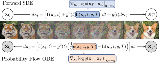
Assuming that the endpoints of a diffusion bridge both exist in and come from an arbitrary and unknown joint distribution, i.e. , we wish to devise a process that learns to approximately sample from by reversing the diffusion bridge with boundary distribution , given a training set of paired samples drawn from .
3.1 Time-Reversed SDE and Probability Flow ODE
Inspired by diffusion bridges, we construct the stochastic process with marginal distribution such that approximates . Reversing the process amounts to sampling from . Note that distribution is different from , i.e. the diffusion marginal distribution, in that the endpoint distributions are now instead of the distribution of a diffusion , which defines a Gaussian given . We can construct the time-reversed SDE/probability flow ODE of via the following theorem.
Theorem 1.
The evolution of conditional probability has a time-reversed SDE of the form
| (6) |
with an associated probability flow ODE
| (7) |
on for any , where denotes a Wiener process, and is as defined in Eq. (5).
A schematic of the bridge process is shown in Figure 1. Note that this process is defined up to . To recover the initial distribution in the SDE case, we make an approximation that for some small simulate SDE backward in time. For the ODE case, since we need to sample from which cannot be Dirac delta, we cannot approximate with a single . Instead, we can first approximate where , and then take an Euler-Maruyama step to , and Eq. (7) can be used afterward. A toy visualization of VE bridge and VP bridges are shown in Figure 2. The top and bottom shows the respective SDE and ODE paths for VE and VP bridges.


3.2 Marginal Distributions and Denoising Bridge Score Matching
The sampling process in Theorem 1 requires approximation of the score where . However, as the true score is not known in closed-form, we take inspiration from denoising score-matching (Song et al., 2020b) and use a neural network to approximate the true score by matching against a tractable quantity. This usually results in closed-form marginal sampling of given data (e.g. in the case of diffusion models and in our case), and given , the model is trained to match against the closed-form denoising score objective. We are motivated to follow a similar approach because (1) tractable marginal sampling of and (2) closed-form objectives enable a simple and scalable algorithm. We specify how to design the marginal sampling distribution and the tractable score objective below to approximate the ground-truth conditional score .
| VP | |||||
| VE |
Sampling distribution. Fortunately, for the former condition, we can design our sampling distribution such that , where is the diffusion distribution pinned at both endpoints as in Eq. (5). For diffusion processes with Gaussian transition kernels, e.g. VE, VP (Song et al., 2020b), our sampling distribution is a Gaussian distribution of the form
| (8) | ||||
where and are pre-defined signal and noise schedules and is the signal-to-noise ratio at time . For VE schedule, we assume and derivation details are provided in Appendix A.1. Notably, the mean of this distribution is a linear interpolation between the (scaled) endpoints, and the distribution approaches a Dirac distribution when nearing either end. For concreteness, we present the bridge processes generated by both VP and VE diffusion in Table 1 and recommend choosing and specified therein.
Training objective. For the latter condition, diffusion bridges benefit from a similar setup as in diffusion models, since a pre-defined signal/noise schedule gives rise to a closed-form conditional score . We show in the following theorem that with , a neural network that matches against this closed-form score approximates the true score.
Theorem 2 (Denoising Bridge Score Matching).
Let , , for any non-zero time sampling distribution in , and be a non-zero loss weighting term of any choice. Minimum of the following objective:
| (9) |
satisfies .
In short, we establish a tractable diffusion bridge over two endpoints and, by matching the conditional score of the Gaussian bridge, we can learn the score of the new distribution that satisfies the boundary distribution .
4 Generalized Parameterization for Distribution Translation
Building the bridge process upon diffusion process allows us to further adapt many recent advancements in the score network parameterization (Ho et al., 2020; Song et al., 2020b; Salimans and Ho, 2022; Ho et al., 2022; Karras et al., 2022), different noise schedules, and efficient ODE sampling (Song et al., 2020a; Karras et al., 2022; Lu et al., 2022a; b; Zhang and Chen, 2022) to our more general framework. Among these works, EDM (Karras et al., 2022) proposes to parameterize the model output to be where is a neural network with parameter that predicts . In a similar spirit, we adopt this pred- parameterization and additionally derive a set of scaling functions for distribution translation, which we show is a strict superset.
Score reparameterization. Following the sampling distribution proposed in (8), a pred- model can predict bridge score by
| (10) |
Scaling functions and loss weighting. Following Karras et al. (2022), and let , , , the scaling functions and weighting function can be derived to be
| (11) | |||
| (12) |
where , , and denote the variance of , variance of , and the covariance of the two, respectively. The only additional hyperparameters compared to EDM are and , which characterize the distribution of and its correlation with . One can notice that in the case of EDM, , because for some Gaussian noise , , and . One can show that the scaling functions then reduce to those in EDM. We leave details in Appendix A.5.
Generalized time-reversal. Due to the probability flow ODE’s resemblance with classifier-guidance (Dhariwal and Nichol, 2021; Ho and Salimans, 2022), we can introduce an additional parameter to set the "strength" of drift adjustment as below.
| (13) |
which allows for a strictly wider class of marginal density of generated by the resulting probability flow ODE. We examine the effect of this parameter in our ablation studies.
5 Stochastic Sampling for Denoising Diffusion Bridges
Although the probability flow ODE allows for one to use fast integration techniques to accelerate the sampling process (Zhang and Chen, 2022; Song et al., 2020a; Karras et al., 2022), purely following an ODE path is problematic because diffusion bridges have fixed starting points given as data , and following the probability flow ODE backward in time generates a deterministic "expected" path. This can result in "averaged" or blurry outputs given initial conditions. Thus, we are motivated to introduce noise into our sampling process to improve the sampling quality and diversity.
Higher-order hybrid sampler. Our sampler is built upon prior higher-order ODE sampler in (Karras et al., 2022), which discretizes the sampling steps into with decreasing intervals (see Appendix A.6 for details). Inspired by the predictor-corrector sampler introduced by Song et al. (2020b), we additionally introduce a scheduled Euler-Maruyama step which follows the backward SDE in between higher-order ODE steps. This ensures that the marginal distribution at each step approximately stays the same. We introduce additional scaling hyperparameter , which define a step ratio in between and such that the interval is used for Euler-Maruyama steps and is used for Heun steps, as described in Algorithm 1.
6 Related Works and Special Cases
Diffusion models. The advancements in diffusion models (Sohl-Dickstein et al., 2015; Ho et al., 2020; Song et al., 2020b) have improved state-of-the-art in image generation and outperformed GANs (Goodfellow et al., 2014). The success of diffusion models goes hand in hand with important design choices such as network design (Song et al., 2020b; Karras et al., 2022; Nichol and Dhariwal, 2021; Hoogeboom et al., 2023; Peebles and Xie, 2023), improved noise-schedules (Nichol and Dhariwal, 2021; Karras et al., 2022; Peebles and Xie, 2023), faster and more accurate samplers (Song et al., 2020a; Lu et al., 2022a; b; Zhang and Chen, 2022), and guidance methods (Dhariwal and Nichol, 2021; Ho and Salimans, 2022). Given the large body of literature on diffusion models for unconditional generation, which largely is based on these various design choices, we seek to design our bridge formulation to allow for a seamless integration with this literature. As such, we adopt a time-reversal perspective to directly extend these methods.
Diffusion bridges, Schödinger bridges, and Doob’s h-transform. Diffusion bridges (Särkkä and Solin, 2019) are a common tool in probability theory and have been actively studied in recent years in the context of generative modeling (Liu et al., 2022b; Somnath et al., 2023; De Bortoli et al., 2021; Peluchetti, ; Peluchetti, 2023). Heng et al. (2021) explores diffusion bridges conditioned on fixed starting/ending points and learns to simulate the time-reversal of the bridge given an approximation of the score . More recently, instead of considering bridges with fixed endpoints, Liu et al. (2022b) uses Doob’s h-transform to bridge between arbitrary distributions. A forward bridge is learned via score-matching by simulating entire paths during training. In contrast, other works (Somnath et al., 2023; Peluchetti, ), while also adopting Doob’s h-transform, propose simulation-free algorithms for forward-time generation. Delbracio and Milanfar (2023) similarly constructs a Brownian Bridge for direct iteration and is successfully applied to image-restoration tasks. Another approach De Bortoli et al. (2021) proposes Iterative Proportional Fitting (IPF) to tractably solve Schödinger Bridge (SB) problems in translating between different distributions. Liu et al. (2023) is built on a tractable class of SB which results in a simulation-free algorithm and has demonstrated strong performance in image translation tasks. More recently, extending SB with IPF, Bridge-Matching (Shi et al., 2023) proposes to use Iterative Markovian Fitting to solve the SB problem. A similar algorithm is also developed by Peluchetti (2023) for distribution translation. A more related work to ours is Li et al. (2023), which proposes to directly reverse a Brownian Bridge for distribution translation in discrete time. Our method instead shows how to construct a bridge model from any existing VP and VE diffusion processes in continuous time, and Brownian Bridge (as considered in most previous works) is but a special case of VE bridges. We additionally show that, when implemented correctly, VP bridges can achieve very strong empirical performance. Although similar perspective can be derived using forward-time diffusion as in Peluchetti which also proposes VE/VP bridge schedules, our framework enjoys additional empirical (reusing diffusion designs) and theoretical (connection with OT-Flow-Matching(Lipman et al., 2023; Tong et al., 2023b) and Rectified Flow (Liu et al., 2022a)) benefits.
Flow and Optimal Transport Works based on Flow-Matching (Lipman et al., 2023; Tong et al., 2023b; Pooladian et al., 2023; Tong et al., 2023a) learn an ODE-based transport map to bridge two distributions. Lipman et al. (2023) has demonstrated that by matching the velocity field of predefined transport maps, one can create powerful generative models competitive with the diffusion counterparts. Improving this approach, Tong et al. (2023b); Pooladian et al. (2023) exploit potential couplings between distributions using minibatch simulation-free OT. Rectified Flow (Liu et al., 2022a) directly constructs the OT bridge and uses neural networks to fit the intermediate velocity field. Another line of work uses stochastic interpolants (Albergo and Vanden-Eijnden, 2023) to build flow models and directly avoid the use of Doob’s h-functions and provide an easy way to construct interpolation maps between distributions. Albergo et al. (2023) presents a general theory with stochastic interpolants unifying flow and diffusion, and shows that a bridge can be constructed from both an ODE and SDE perspctive. Separate from these methods, our model uses a different denoising bridge score-matching loss than this class of models. Constructing from this perspective allows us to extend many existing successful designs of diffusion models (which are not directly applicable to these works) to the bridge framework and push state-of-the-art further for image translation while retaining strong performance for unconditional generation.
6.1 Special Cases of Denoising Diffusion Bridge Models
Case 1: Unconditional diffusion process (Song et al., 2020b). For unconditional diffusion processes (which map data to noise), we can first show that the marginal when exactly matches that of a regular diffusion process when . By taking expectation over in Eq. (8), we have
| (14) |
One can further show that during sampling, Eq. (6) and (7) reduce to the reverse SDE and ODE (respectively) of a diffusion process when is sampled from a Gaussian. We leave derivation details to Appendix A.4.
Case 2: OT-Flow-Matching (Lipman et al., 2023; Tong et al., 2023b) and Rectified Flow (Liu et al., 2022a). These works learn to match deterministic dynamics defined through ODEs instead of SDEs. In this particular case, they work with “straight line" paths defined by .
To see that our framework generalizes this, first let us define a family of diffusion bridges with variance scaled by such that where and are as defined in Eq. (8). One can therefore show that with a VE diffusion where , given some fixed and , i.e. , and sampled from Eq. (8),
| (15) |
where inside the bracket is the drift of probability flow ODE in Eq. (7) given and , and the right hand side is exactly the straight line path term. In other words, these methods learn to match the drift in the bridge probability flow ODE (with a specific VE schedule) in the noiseless limit. The score model can then be matched against , with some additional caveat to handle additional input , our framework exactly reduces to that of OT-Flow-Matching and Rectified Flow (details in Appendix A.4).
7 Experiments
In this section we verify the generative capability of DDBM , and we want to answer the following questions: (1) How well does DDBM perform in image-to-image translation in pixel space? (2) Can DDBM perform well in unconditional generation when one side of the bridge reduces to Gaussian distribution? (3) How does the additional design choices introduced affect the final performance? Unless noted otherwise, we use the same VE diffusion schedule as in EDM for our bridge model by default. We leave further experiment details to Appendix B.
| Condition | Pix2Pix [16] | SDEdit [28] | Rectified Flow [24] | I2SB [23] | DDBM (VE), ODE sampler | DDBM (VE), hybrid sampler |
|---|
7.1 Image-to-Image Translation
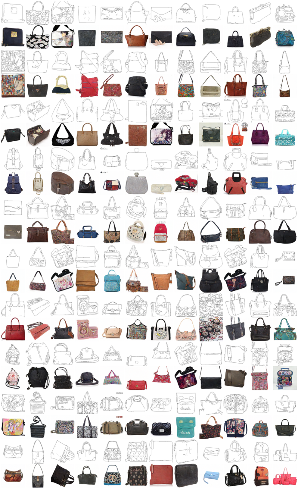
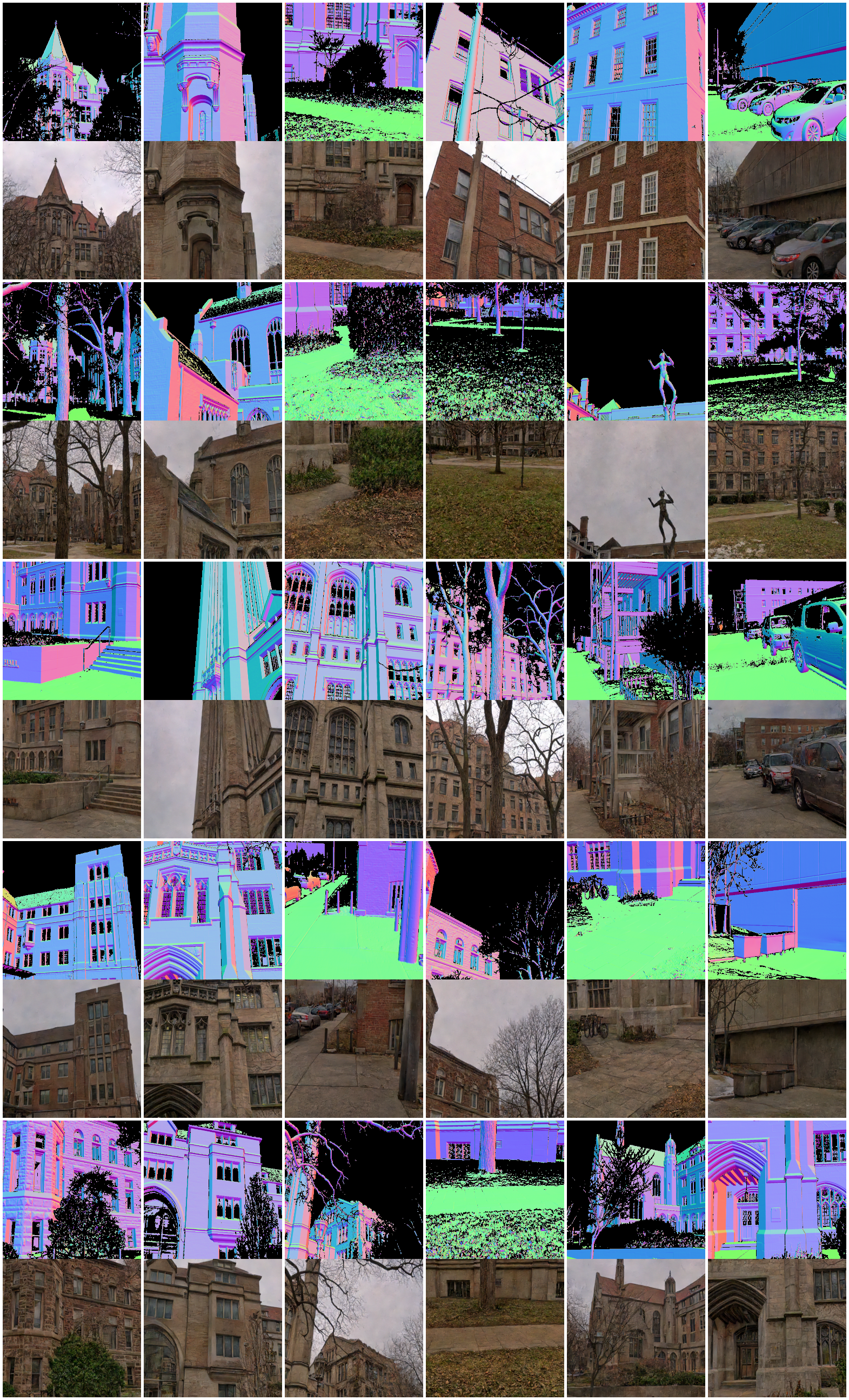
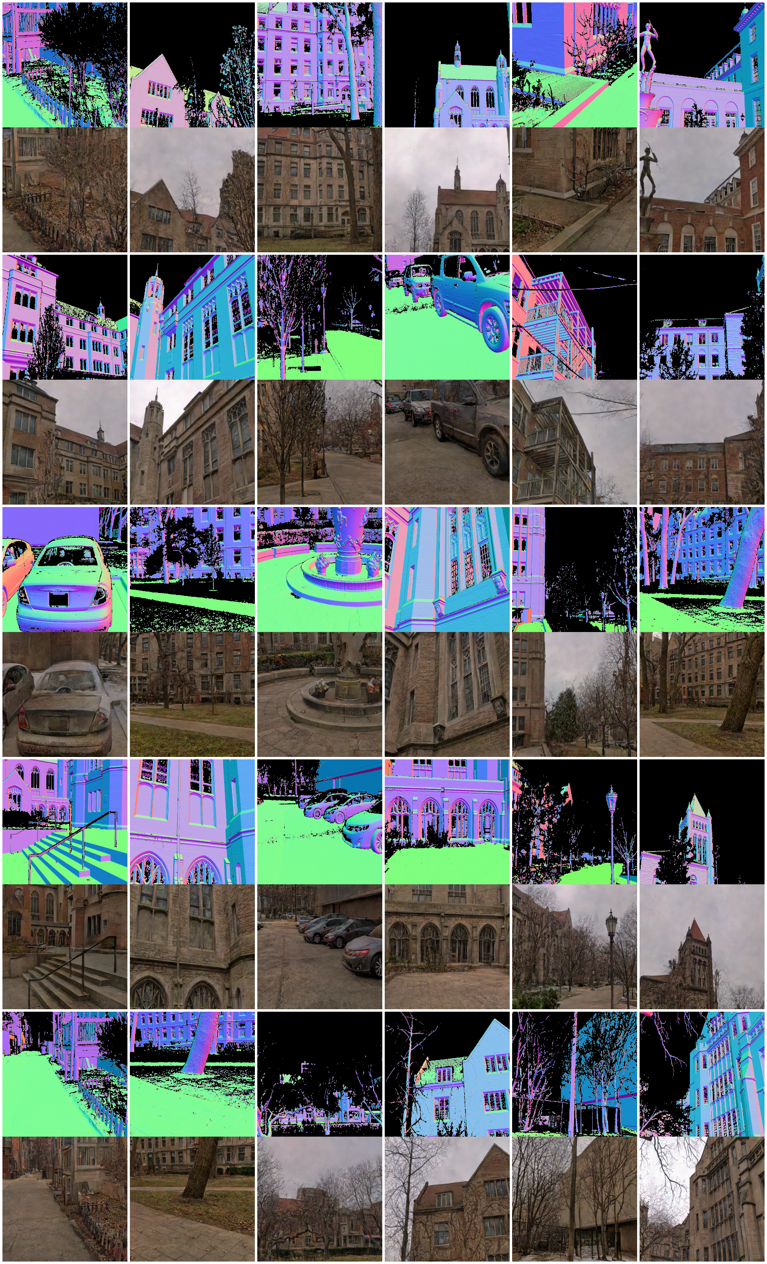
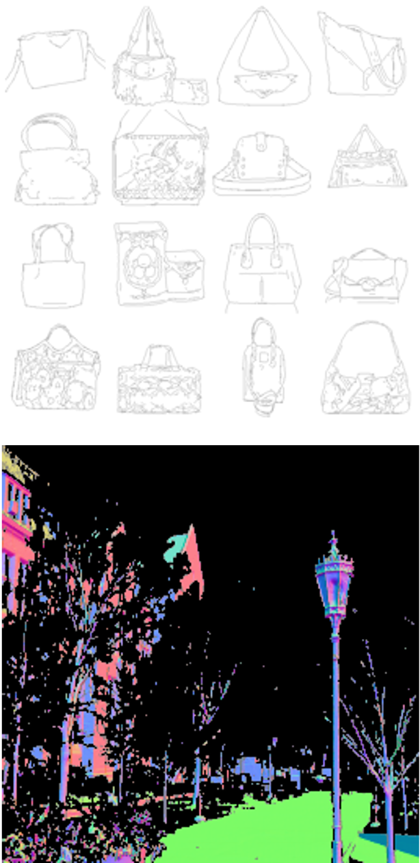
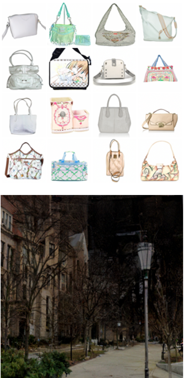
We demonstrate that DDBM can deliver competitive results in general image-to-image translation tasks. We evaluate on datasets with different image resolutions to demonstrate its applicability on a variety of scales. We choose EdgesHandbags (Isola et al., 2017) scaled to pixels, which contains image pairs for translating from edge maps to colored handbags, and DIODE-Outdoor (Vasiljevic et al., 2019) scaled to , which contains normal maps and RGB images of real-world outdoor scenes. For evaluation metrics, we use Fréchet Inception Distance (FID) (Heusel et al., 2017) and Inception Scores (IS) (Barratt and Sharma, 2018) evaluated on all training samples translation quality, and we use LPIPS (Zhang et al., 2018) and MSE (in scale) to measure perceptual similarity and translation faithfulness.
We compare with Pix2Pix (Isola et al., 2017), SDEdit (Meng et al., 2022), DDIB (Su et al., 2022), Rectified Flow (Liu et al., 2022a), and I2SB (Liu et al., 2023) as they are built for image-to-image translation. For SDEdit we train unconditional EDM on the target domain, e.g. colored images, and initialize the translation by noising source image, e.g. sketches, and generate by EDM sampler given the noisy image. The other baseline methods are run with their respective repo while using the same network architecture as ours. Diffusion and transport-based methods are evaluated with the same number of function evaluations (, which is the default for EDM sampler for images) to demonstrate our sampler’s effectiveness in the regime when the number of sampling steps are low. Results are shown in Table 2 and additional settings are specified in Appendix B.
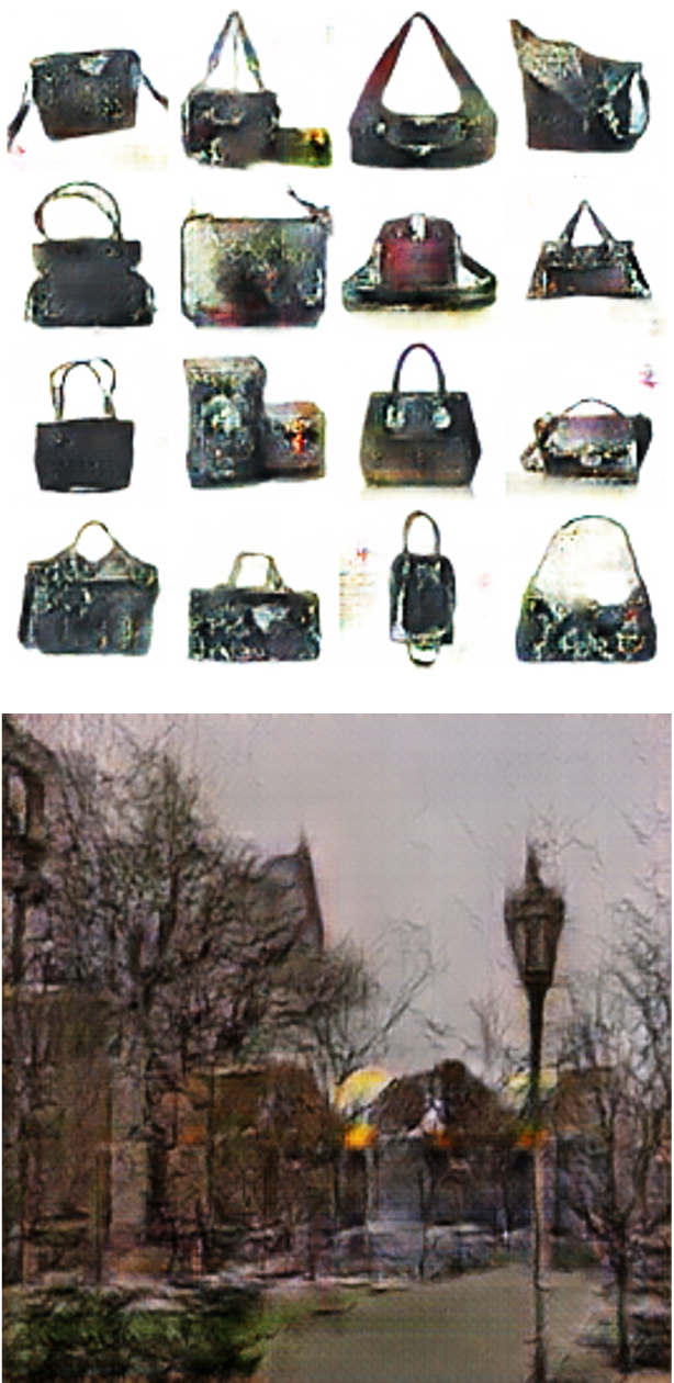
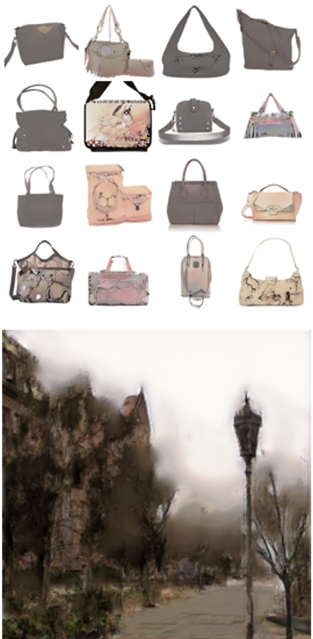
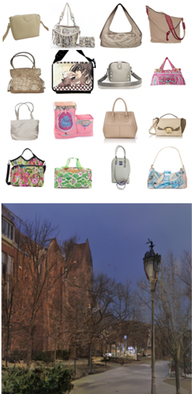
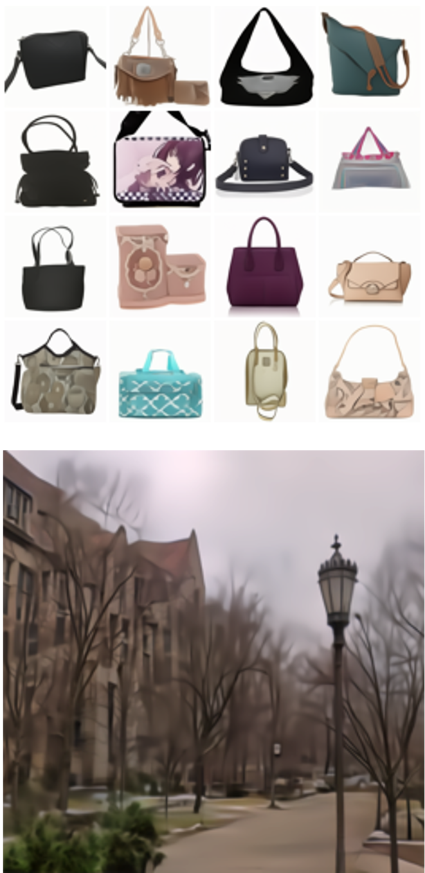
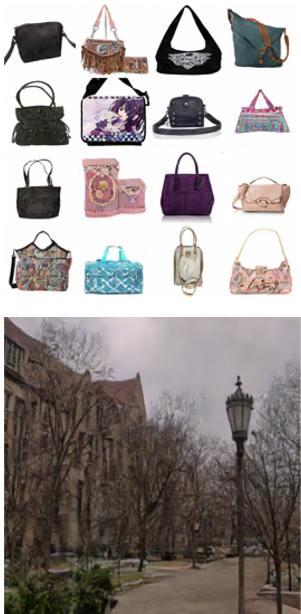
We observe that our model can perform translation with both high generation quality and faithfulness, and we find that VP bridges outperform VE bridges in some cases. In contrast, Rectified-Flow as an OT-based method struggles to perform well when the two domains share little low-level similarities (e.g. color, hue). DDIB also fails to produce coherent translation due to the wide differences in pixel-space distribution between the paired data. I2SB comes closest to our method, but falls short when limited by computational constraints, i.e. NFE is low. We additionally show qualitative comparison with the most performant baselines in Figure 3. More visual results can be found in Appendix B.1.
7.2 Ablation Studies
We now study the effect of our preconditioning and hybrid samplers on generation quality in the context of both VE and VP bridge (see Appendix B for VP bridge parameterization). In the left column of Figure 4, we fix the guidance scale at 1 and vary the Euler step size from 0 to 0.9 to introduce stochasticity. We see a significant decrease in FID score as we increase which produces the best performance at some value between 0 and 1 (e.g. for EdgesHandbags). Figure 3 also shows that the ODE sampler (i.e. ) produces blurry images while our hybrid sampler produces considerably sharper results. On the right column, we study the effect of (from 0 to 1) with fixed . We observe that VE bridges are not affected by the change in whereas VP bridges heavily rely on setting . We hypothesize that this is due to the fact that VP bridges follow "curved paths" and destroy signals in between, so it is reliant on Doob’s -function for further guidance towards correct probability distribution.
We also study the effect of our preconditioning in Table 3. Our baseline without our preconditioning and our sampler is a simple model that directly matches output of the neural network to the training target and generates using EDM (Karras et al., 2022) sampler. We see that each introduced component further boosts the generation performance. Therefore, we can conclude that the introduced practical components are essential for the success of our DDBM .
| EdgesHandbags-6464 | DIODE-256256 | |||||||
| FID | IS | LPIPS | MSE | FID | IS | LPIPS | MSE | |
| Pix2Pix (Isola et al., 2017) | 74.8 | 4.24 | 0.356 | 0.209 | 82.4 | 4.22 | 0.556 | 0.133 |
| DDIB (Su et al., 2022) | 186.84 | 2.04 | 0.869 | 1.05 | 242.3 | 4.22 | 0.798 | 0.794 |
| SDEdit (Meng et al., 2022) | 26.5 | 3.58 | 0.271 | 0.510 | 31.14 | 5.70 | 0.714 | 0.534 |
| Rectified Flow (Liu et al., 2022a) | 25.3 | 2.80 | 0.241 | 0.088 | 77.18 | 5.87 | 0.534 | 0.157 |
| I2SB (Liu et al., 2023) | 7.43 | 3.40 | 0.244 | 0.191 | 9.34 | 5.77 | 0.373 | 0.145 |
| DDBM (VE) | 2.93 | 3.58 | 0.131 | 0.013 | 8.51 | 6.03 | 0.226 | 0.0107 |
| DDBM (VP) | 1.83 | 3.73 | 0.142 | 0.0402 | 4.43 | 6.21 | 0.244 | 0.0839 |


| Our precond. | Our sampler | EH-6464 | DIODE-256256 | ||
|---|---|---|---|---|---|
| VE | VP | VE | VP | ||
| ✗ | ✗ | 14.02 | 11.76 | 126.3 | 96.93 |
| ✓ | ✗ | 13.26 | 11.19 | 79.25 | 91.07 |
| ✗ | ✓ | 13.11 | 29.91 | 91.31 | 21.92 |
| ✓ | ✓ | 2.93 | 1.83 | 8.51 | 4.43 |
7.3 Unconditional Generation
When one side of the distribution becomes Gaussian distribution, our framework exactly reduces to that of diffusion models. Specifically, during training when the end point , our intermediate bridge samples follows the distribution . We empirically verify that using our bridge sampling and the pred- objective inspired by EDM, we can recover its performance by using our more generalized parameterization.
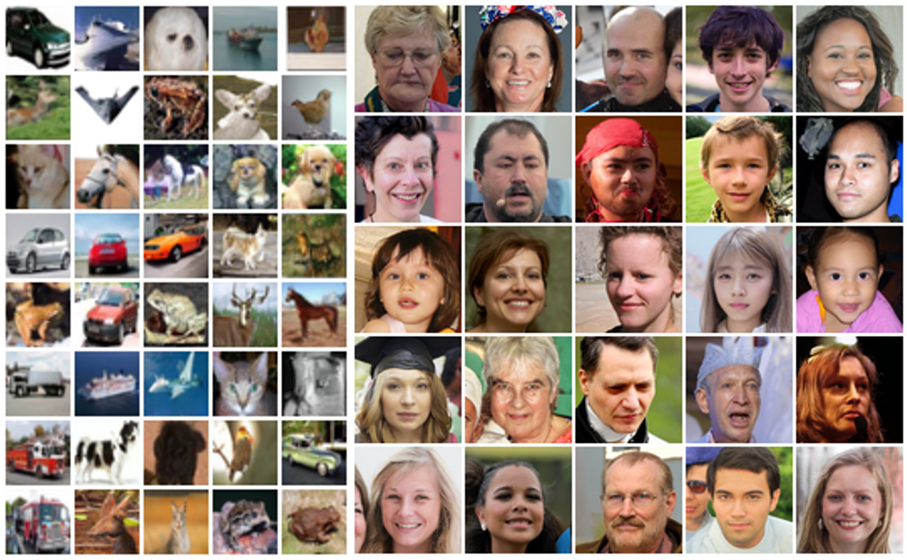
We evaluate our method on CIFAR-10 (Krizhevsky et al., 2009) and FFHQ- (Karras et al., 2019) which are processed according to Karras et al. (2022). We use FID score for quantitative evaluation using 50K generated images and use number of function evaluations (NFE) for generation efficiency. We compare our generation results against diffusion-based and optimal transport-based models including DDPM (Ho et al., 2020), DDIM (Song et al., 2020a), DDPM++ (Song et al., 2020b), NCSN++ (Song et al., 2020b), Rectified Flow (Liu et al., 2022a), EDM (Karras et al., 2022). Quantitative results are presented in Table 4 and generated samples are shown in Figure 5.
We observe that our model is able to match EDM performance with negligible degradation in FID scores for CIFAR-10 and marginal improvement for FFHQ-. This corroborates our claim that our method can benefit from advances in diffusion models and generalize many of the advanced parameterization techniques such as those introduced in EDM.
8 Conclusion
In this work, we introduce Denoising Diffusion Bridge Models, a novel class of models that builds a stochastic bridge between paired samples with tractable marginal distributions in between. The model is learned by matching the conditional score of a tractable bridge distribution, which allows one to transport from one distribution to another via a new reverse SDE or probability flow ODE. Additionally, this generalized framework shares many similarities with diffusion models, thus allowing us to reuse and generalize many designs of diffusion models. We believe that DDBM is a significant contribution towards a general framework for distribution translation. In the era of generative AI, DDBM has a further role to play.
References
- Albergo et al. [2023] Michael S Albergo, Nicholas M Boffi, and Eric Vanden-Eijnden. Stochastic interpolants: A unifying framework for flows and diffusions. arXiv preprint arXiv:2303.08797, 2023.
- Albergo and Vanden-Eijnden [2023] Michael Samuel Albergo and Eric Vanden-Eijnden. Building normalizing flows with stochastic interpolants. In The Eleventh International Conference on Learning Representations, 2023. URL https://openreview.net/forum?id=li7qeBbCR1t.
- Barratt and Sharma [2018] Shane Barratt and Rishi Sharma. A note on the inception score. arXiv preprint arXiv:1801.01973, 2018.
- De Bortoli et al. [2021] Valentin De Bortoli, James Thornton, Jeremy Heng, and Arnaud Doucet. Diffusion schrödinger bridge with applications to score-based generative modeling. Advances in Neural Information Processing Systems, 34:17695–17709, 2021.
- Delbracio and Milanfar [2023] Mauricio Delbracio and Peyman Milanfar. Inversion by direct iteration: An alternative to denoising diffusion for image restoration. arXiv preprint arXiv:2303.11435, 2023.
- Delyon and Hu [2006] Bernard Delyon and Ying Hu. Simulation of conditioned diffusion and application to parameter estimation. Stochastic Processes and their Applications, 116(11):1660–1675, 2006.
- Dhariwal and Nichol [2021] Prafulla Dhariwal and Alexander Nichol. Diffusion models beat gans on image synthesis. Advances in Neural Information Processing Systems, 34:8780–8794, 2021.
- Doob and Doob [1984] Joseph L Doob and JI Doob. Classical potential theory and its probabilistic counterpart, volume 262. Springer, 1984.
- Goodfellow et al. [2014] Ian J. Goodfellow, Jean Pouget-Abadie, Mehdi Mirza, Bing Xu, David Warde-Farley, Sherjil Ozair, Aaron C. Courville, and Yoshua Bengio. Generative adversarial nets. In NIPS, 2014.
- Heng et al. [2021] Jeremy Heng, Valentin De Bortoli, Arnaud Doucet, and James Thornton. Simulating diffusion bridges with score matching. arXiv preprint arXiv:2111.07243, 2021.
- Heusel et al. [2017] Martin Heusel, Hubert Ramsauer, Thomas Unterthiner, Bernhard Nessler, and Sepp Hochreiter. Gans trained by a two time-scale update rule converge to a local nash equilibrium. Advances in neural information processing systems, 30, 2017.
- Ho and Salimans [2022] Jonathan Ho and Tim Salimans. Classifier-free diffusion guidance. arXiv preprint arXiv:2207.12598, 2022.
- Ho et al. [2020] Jonathan Ho, Ajay Jain, and Pieter Abbeel. Denoising diffusion probabilistic models. Advances in Neural Information Processing Systems, 33:6840–6851, 2020.
- Ho et al. [2022] Jonathan Ho, William Chan, Chitwan Saharia, Jay Whang, Ruiqi Gao, Alexey Gritsenko, Diederik P Kingma, Ben Poole, Mohammad Norouzi, David J Fleet, et al. Imagen video: High definition video generation with diffusion models. arXiv preprint arXiv:2210.02303, 2022.
- Hoogeboom et al. [2023] Emiel Hoogeboom, Jonathan Heek, and Tim Salimans. simple diffusion: End-to-end diffusion for high resolution images. arXiv preprint arXiv:2301.11093, 2023.
- Isola et al. [2017] Phillip Isola, Jun-Yan Zhu, Tinghui Zhou, and Alexei A Efros. Image-to-image translation with conditional adversarial networks. In Proceedings of the IEEE conference on computer vision and pattern recognition, pages 1125–1134, 2017.
- Karras et al. [2019] Tero Karras, Samuli Laine, and Timo Aila. A style-based generator architecture for generative adversarial networks. In Proceedings of the IEEE/CVF conference on computer vision and pattern recognition, pages 4401–4410, 2019.
- Karras et al. [2022] Tero Karras, Miika Aittala, Timo Aila, and Samuli Laine. Elucidating the design space of diffusion-based generative models. arXiv preprint arXiv:2206.00364, 2022.
- Kingma et al. [2021] Diederik Kingma, Tim Salimans, Ben Poole, and Jonathan Ho. Variational diffusion models. Advances in neural information processing systems, 34:21696–21707, 2021.
- Krizhevsky et al. [2009] Alex Krizhevsky, Geoffrey Hinton, et al. Learning multiple layers of features from tiny images. 2009.
- Li et al. [2023] Bo Li, Kaitao Xue, Bin Liu, and Yu-Kun Lai. Bbdm: Image-to-image translation with brownian bridge diffusion models. In Proceedings of the IEEE/CVF Conference on Computer Vision and Pattern Recognition, pages 1952–1961, 2023.
- Lipman et al. [2023] Yaron Lipman, Ricky T. Q. Chen, Heli Ben-Hamu, Maximilian Nickel, and Matthew Le. Flow matching for generative modeling. In The Eleventh International Conference on Learning Representations, 2023. URL https://openreview.net/forum?id=PqvMRDCJT9t.
- Liu et al. [2023] Guan-Horng Liu, Arash Vahdat, De-An Huang, Evangelos A Theodorou, Weili Nie, and Anima Anandkumar. I2sb: Image-to-image schrödinger bridge. arXiv, 2023.
- Liu et al. [2022a] Xingchao Liu, Chengyue Gong, and Qiang Liu. Flow straight and fast: Learning to generate and transfer data with rectified flow. arXiv preprint arXiv:2209.03003, 2022a.
- Liu et al. [2022b] Xingchao Liu, Lemeng Wu, Mao Ye, and Qiang Liu. Let us build bridges: Understanding and extending diffusion generative models. arXiv preprint arXiv:2208.14699, 2022b.
- Lu et al. [2022a] Cheng Lu, Yuhao Zhou, Fan Bao, Jianfei Chen, Chongxuan Li, and Jun Zhu. Dpm-solver: A fast ode solver for diffusion probabilistic model sampling in around 10 steps. arXiv preprint arXiv:2206.00927, 2022a.
- Lu et al. [2022b] Cheng Lu, Yuhao Zhou, Fan Bao, Jianfei Chen, Chongxuan Li, and Jun Zhu. Dpm-solver++: Fast solver for guided sampling of diffusion probabilistic models. arXiv preprint arXiv:2211.01095, 2022b.
- Meng et al. [2022] Chenlin Meng, Yutong He, Yang Song, Jiaming Song, Jiajun Wu, Jun-Yan Zhu, and Stefano Ermon. SDEdit: Guided image synthesis and editing with stochastic differential equations. In International Conference on Learning Representations, 2022.
- Nichol and Dhariwal [2021] Alexander Quinn Nichol and Prafulla Dhariwal. Improved denoising diffusion probabilistic models. In International Conference on Machine Learning, pages 8162–8171. PMLR, 2021.
- Peebles and Xie [2023] William Peebles and Saining Xie. Scalable diffusion models with transformers. In Proceedings of the IEEE/CVF International Conference on Computer Vision, pages 4195–4205, 2023.
- [31] Stefano Peluchetti. Non-denoising forward-time diffusions.
- Peluchetti [2023] Stefano Peluchetti. Diffusion bridge mixture transports, schr" odinger bridge problems and generative modeling. arXiv preprint arXiv:2304.00917, 2023.
- Pooladian et al. [2023] Aram-Alexandre Pooladian, Heli Ben-Hamu, Carles Domingo-Enrich, Brandon Amos, Yaron Lipman, and Ricky Chen. Multisample flow matching: Straightening flows with minibatch couplings. arXiv preprint arXiv:2304.14772, 2023.
- Ramesh et al. [2022] Aditya Ramesh, Prafulla Dhariwal, Alex Nichol, Casey Chu, and Mark Chen. Hierarchical text-conditional image generation with clip latents. ArXiv, abs/2204.06125, 2022.
- Rogers and Williams [2000] L Chris G Rogers and David Williams. Diffusions, Markov processes and martingales: Volume 2, Itô calculus, volume 2. Cambridge university press, 2000.
- Rombach et al. [2022] Robin Rombach, Andreas Blattmann, Dominik Lorenz, Patrick Esser, and Björn Ommer. High-resolution image synthesis with latent diffusion models. In Proceedings of the IEEE/CVF Conference on Computer Vision and Pattern Recognition, pages 10684–10695, 2022.
- Saharia et al. [2021] Chitwan Saharia, William Chan, Huiwen Chang, Chris A. Lee, Jonathan Ho, Tim Salimans, David J. Fleet, and Mohammad Norouzi. Palette: Image-to-image diffusion models. ACM SIGGRAPH 2022 Conference Proceedings, 2021.
- Salimans and Ho [2022] Tim Salimans and Jonathan Ho. Progressive distillation for fast sampling of diffusion models. arXiv preprint arXiv:2202.00512, 2022.
- Särkkä and Solin [2019] Simo Särkkä and Arno Solin. Applied stochastic differential equations, volume 10. Cambridge University Press, 2019.
- Schauer et al. [2017] Moritz Schauer, Frank Van Der Meulen, and Harry Van Zanten. Guided proposals for simulating multi-dimensional diffusion bridges. 2017.
- Shi et al. [2023] Yuyang Shi, Valentin De Bortoli, Andrew Campbell, and Arnaud Doucet. Diffusion schr" odinger bridge matching. arXiv preprint arXiv:2303.16852, 2023.
- Sohl-Dickstein et al. [2015] Jascha Sohl-Dickstein, Eric Weiss, Niru Maheswaranathan, and Surya Ganguli. Deep unsupervised learning using nonequilibrium thermodynamics. In International Conference on Machine Learning, pages 2256–2265. PMLR, 2015.
- Somnath et al. [2023] Vignesh Ram Somnath, Matteo Pariset, Ya-Ping Hsieh, Maria Rodriguez Martinez, Andreas Krause, and Charlotte Bunne. Aligned diffusion schr" odinger bridges. arXiv preprint arXiv:2302.11419, 2023.
- Song et al. [2020a] Jiaming Song, Chenlin Meng, and Stefano Ermon. Denoising diffusion implicit models. arXiv preprint arXiv:2010.02502, 2020a.
- Song and Ermon [2019] Yang Song and Stefano Ermon. Generative modeling by estimating gradients of the data distribution. Advances in neural information processing systems, 32, 2019.
- Song et al. [2020b] Yang Song, Jascha Sohl-Dickstein, Diederik P Kingma, Abhishek Kumar, Stefano Ermon, and Ben Poole. Score-based generative modeling through stochastic differential equations. arXiv preprint arXiv:2011.13456, 2020b.
- Su et al. [2022] Xuan Su, Jiaming Song, Chenlin Meng, and Stefano Ermon. Dual diffusion implicit bridges for image-to-image translation. In The Eleventh International Conference on Learning Representations, 2022.
- Szavits-Nossan and Evans [2015] Juraj Szavits-Nossan and Martin R Evans. Inequivalence of nonequilibrium path ensembles: the example of stochastic bridges. Journal of Statistical Mechanics: Theory and Experiment, 2015(12):P12008, 2015.
- Tong et al. [2023a] Alexander Tong, Nikolay Malkin, Kilian Fatras, Lazar Atanackovic, Yanlei Zhang, Guillaume Huguet, Guy Wolf, and Yoshua Bengio. Simulation-free schr" odinger bridges via score and flow matching. arXiv preprint arXiv:2307.03672, 2023a.
- Tong et al. [2023b] Alexander Tong, Nikolay Malkin, Guillaume Huguet, Yanlei Zhang, Jarrid Rector-Brooks, Kilian Fatras, Guy Wolf, and Yoshua Bengio. Improving and generalizing flow-based generative models with minibatch optimal transport. In ICML Workshop on New Frontiers in Learning, Control, and Dynamical Systems, 2023b.
- Vasiljevic et al. [2019] Igor Vasiljevic, Nick Kolkin, Shanyi Zhang, Ruotian Luo, Haochen Wang, Falcon Z. Dai, Andrea F. Daniele, Mohammadreza Mostajabi, Steven Basart, Matthew R. Walter, and Gregory Shakhnarovich. DIODE: A Dense Indoor and Outdoor DEpth Dataset. CoRR, abs/1908.00463, 2019. URL http://arxiv.org/abs/1908.00463.
- Villani [2008] Cédric Villani. Optimal transport: Old and new. 2008.
- Zhang and Chen [2022] Qinsheng Zhang and Yongxin Chen. Fast sampling of diffusion models with exponential integrator. arXiv preprint arXiv:2204.13902, 2022.
- Zhang et al. [2018] Richard Zhang, Phillip Isola, Alexei A Efros, Eli Shechtman, and Oliver Wang. The unreasonable effectiveness of deep features as a perceptual metric. In CVPR, 2018.
- Zhu et al. [2017] Jun-Yan Zhu, Taesung Park, Phillip Isola, and Alexei A. Efros. Unpaired image-to-image translation using cycle-consistent adversarial networks. 2017 IEEE International Conference on Computer Vision (ICCV), pages 2242–2251, 2017.
Appendix: Denoising Diffusion Bridge Models
Appendix A Proofs
A.1 Marginal distribution
We note that for tractable transition kernels specified in Table 1, we can derive the marginal distribution of using Bayes’ rule
We can directly derive this by looking at the resulting density function. First,
| (16) | ||||
| (17) | ||||
| (18) | ||||
| (19) |
and we refer readers to Kingma et al. (2021) for details on for any . Then we know
| (20) | ||||
| (21) |
where
| (22) | ||||
| (23) |
A.2 Denoising Bridge Score Matching
See 2
Proof.
We can explicitly write the objective as
|
|
(24) |
Since the objective is an loss and are non-zero, its minimum can be derived as
| (25) | ||||
| (26) | ||||
| (27) | ||||
| (28) | ||||
| (29) | ||||
| (30) |
Thus, minimizing the objective approximates the conditional score. ∎
A.3 Probability Flow ODE of Diffusion Bridges
See 1
Proof.
To find the time evolution of , we can first find the time evolution of for fixed endpoints and , which by Bayes’ rule is
where follows Kolmogorov forward equation
| (31) |
and follows Kolmogorov backward equation Szavits-Nossan and Evans (2015) where
| (32) |
The time derivative of thus follows
| (33) | ||||
| (34) | ||||
| (35) |
Further expanding the right-hand-side, we have
We can notice that the sum of the first terms of and is the result of a product rule, thus
| (36) |
We now focus on reducing the terms in the last bracket. For clarity, we similarly number the two terms inside the bracket such that
| (37) | ||||
| (38) |
Now we can complete these terms to be results of product rule by adding and subtracting the following term
| (39) | |||
| (40) | |||
| (41) |
which takes 2 equivalent forms and . Now we can write Eq. (36) as
| (42) | ||||
| (43) |
We can notice that
| (44) | ||||
| (45) |
and using Bayes’ rule,
| (46) |
we have
| (47) | ||||
| (48) |
Therefore,
| (49) | ||||
which is a Fokker-Planck equation for a (forward) SDE with the modified drift term
To find the time derivative for , we can simply marginalize out with distribution in the resulting Fokker-Planck, which can be achieved due to linearity of expectation with respect to . That is,
| (50) | ||||
Since for for some , Doob’s h-function is well-defined, and is smooth, and we can take the expectation inside the equations. Additionally, the drift adjustment does not depend on the expectation is simply over expectation and by definition LHS is ,
| (51) | ||||
This characterizes a reverse SDE specified in Theorem 1.
We can further use conversion trick in Song et al. (2020b) to convert this into a continuity equation without any diffusion term where
| (52) |
where
| (53) | ||||
| (54) |
∎
A.4 Special Cases of Denoising Diffusion Bridges
Unconditional diffusion models. We first give a general intuition that the marginal distribution of sampling from the bridge is the same as sampling marginally from for a diffusion transition kernel . We can see this by observing
| (55) |
where . And since we assume we rewrite the above equation as
| (56) | ||||
| (57) | ||||
| (58) |
where and the last equality is due to the fact that the addition of two Gaussian with variances , is another Gaussian with variance .
Formally, to show that it is a special case, we first observe that the score matching objective allows our network to approximate which is the conditional score of the diffusion transition kernel. Then we will show that the Fokker-Planck equation reduces to that of a diffusion when marginalizing out dependency on .
From proof of Theorem 1, we know that the Fokker-Planck equation for follows
| (59) | ||||
| (60) |
Here we note that we use because we are considering a diffusion process as a special case of a general introduced in Theorem 2. We can marginalize out such that
| (61) |
and so
| (62) |
and the second term can be reduced by writing the expectation explicitly as
| (63) | ||||
| (64) | ||||
| (65) | ||||
| (66) | ||||
| (67) |
Therefore, the resulting probability flow ODE is
| (68) |
which is that of a regular diffusion. Therefore, by setting data distribution to be we recover unconditional diffusion models.
OT-Flow Matching and Rectified Flow. As proposed, we use a VE schedule such that and for some constant . Then the probability flow ODE conditioned on becomes
| (69) |
Specifically, the drift term becomes
| (70) |
where . And we can rearrange the terms to be
| (71) | ||||
| (72) | ||||
| (73) |
And by taking , we have for . Therefore the network learns to match this drift term in the noiseless limit of denoising diffusion bridge in OT-Flow Matching and Rectified Flow case.
We next note that the original score-matching loss is no longer valid as bridge noise causes exploding magnitude of bridge score . We can then resort to matching against altogether.
One additional caveat is that our framework as presented needs to take in as an additional condition. To handle this, we note the generalized parameterization can be used to define where is our actual network. We then set and and uses loss , which is the case of OT-Flow-Matching and Rectified Flow.
A.5 Generalized Parameterization
We now derive the EDM scaling functions from first principle, as suggested by (Karras et al., 2022).
Let , , . First, we expand the pred- objective as
where for . To derive , we set the variance of the resulting input to be 1, where
| (74) | ||||
| (75) |
For simplicity we denote the neural network as , and the inner square loss can be expanded to be
| (76) | ||||
| (77) |
And we want the prediction target to have variance 1, thus
| (78) |
and
| (79) |
Following reasoning in Karras et al. (2022), we minimize w.r.t. by taking derivative and set to 0, which is
| (80) |
and this implies
| (81) | ||||
| (82) |
And
| (83) | ||||
| (84) | ||||
| (85) | ||||
| (86) |
Finally, , and for time, we simply reuse that proposed in Karras et al. (2022) as no significant change in time’s distribution.
EDM (Karras et al., 2022) as a special case. In the case of unconditional diffusion models, we have , so and . Additionally, , , . Substituting in these into the coefficients, we have
| (87) | ||||
| (88) | ||||
| (89) | ||||
| (90) | ||||
| (91) | ||||
| (92) | ||||
| (93) | ||||
| (94) | ||||
| (95) |
And .
A.6 Sampler Discretization
EDM introduces Heun sampler, which discretizes the sampling steps into where
| (96) |
and is a default choice. It then integrates over the probability flow ODE path with second-order Heun steps for each such discretization step. We reuse this discretization for all our experiments.
Appendix B Experiment Details
Architecture. For unconditional generation, architectures are reused from Karras et al. (2022) for both CIFAR-10 and FFHQ-6464. For pixel-space translation, we use ADM (Dhariwal and Nichol, 2021) architecture for both 6464 and 256256 resolutions. For latent-space translation, which reduces to 3232 resolution in the latent space, we use ADM (Dhariwal and Nichol, 2021) architecture for 6464 resolution but change the channel dimensions from 192 to 256 and reduce the number of residual blocks from 3 to 2, and we fix everything else to be same as that for 6464 resolution. We use 0.1 dropout for all models. Conditioning is done via concatenation at the input level.
VE and VP bridge parameterization. There are many schedules we can choose for both types of bridges. For all our experiments, VE bridges follow and and VP bridges follow a time-invariant drift . This is a special case of the linear noise schedule considered in Song et al. (2020b) with . We simply choose because this results in a bridge that has symmetric noise levels w.r.t. time. We observe that linearly increasing drift causes the max noise to shift towards a higher and the noise decreases faster to 0 at than for a symmetric bridge. This makes the learning process more difficult and degrades performance.
Training. We use AdamW optimizer with 0.0001 learning rate and no weight decay. The batch size is 256 for all image size less than 256 and training is done on 4 NVIDIA A100 40G. For 256256 resolution, the batch size is 4 accumulated 4 times such that the effective batch size is 64, trained on 4 NVIDIA A100 40G. The training is terminated at 500K iterations. During training, for image-to-image translation, we set , , and for unconditional generation, we set , and . We use random flipping as our data augmentation for image-to-image translation and reuse augmentation from Karras et al. (2022) for generation.
Baselines. All baselines are trained using the same architecture as ours for each experiment. For SDEdit, we use pretrained EDM model on and conduct image-to-image translation by first noising and denoising using the pretrained model. We reuse the noise schedule proposed by (Karras et al., 2022) and for reasonable generation while retaining global structure of the image conditions, we noise using the noise variance indexed at 1/3 of EDM noise schedule and denoise starting from this noised image for the remaining 1/3 of total of steps. For DDIB, we train two separate unconditional models starting for and separately and perform translation by reversing DDIM starting from and generating using DDIM for . We reuse the original baseline code for all baselines while.
Sampling. For all experiments we evaluate models on a low-step regime, i.e. the same number of sampling steps. For all experiments, we set guidance scale and for image translation and unconditional generation, we use euler step ratio ratio and respectively. In case of , no Euler step is done. With these settings, we set , or , for 3232 resolution image translation, and for all other resolutions, we use , or , for image translation. For unconditional generation, for CIFAR-10 and for FFHQ-6464. FID and IS scores are calculated using the entire training set for all datasets for image translation tasks. They are calculated using 50K samples for unconditional generation tasks.
B.1 Additional Results.
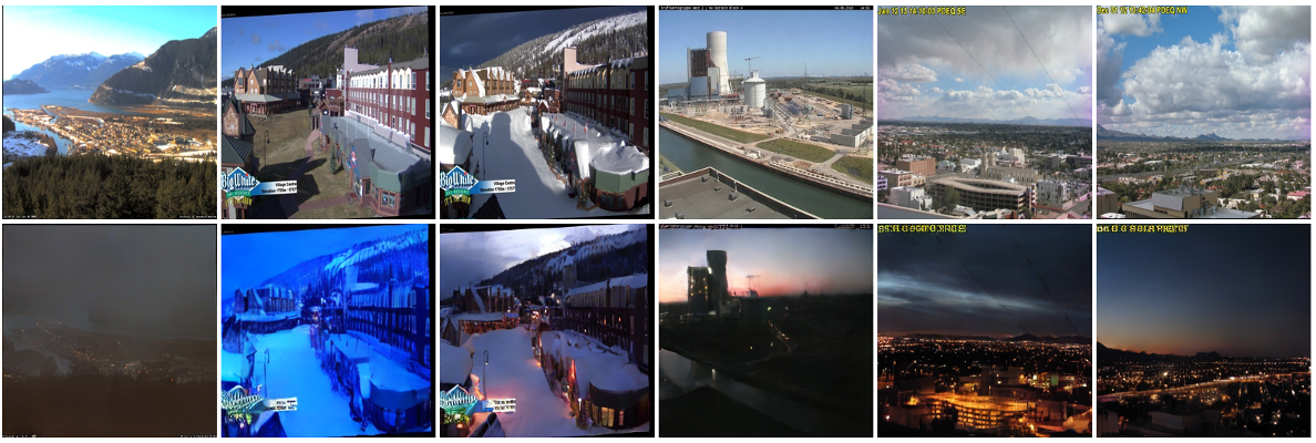
Latent space translation. Many real world applications of diffusion models rely on the existence of a latent space (Rombach et al., 2022), which significantly relieves computational burden in practice. We thus also investigate whether DDBM can naturally adapt to latent space translation tasks. We conduct our experiment on DayNight (Isola et al., 2017) which is chosen because we observe that the autoencoder presented in Rombach et al. (2022) with factor 8 resolution reduction can faithfully reconstruct the dataset in high quality. We reuse the metrics and baselines from before, and we evaluate all models with using the EDM sampler default for images, which is the size for the latent space. To isolate the evaluation for latent space translation, we use the reconstructed ground-truths by the autoencoder as our pseudo ground-truths against which the decoded samples are compared for all metrics. Quantitative results are presented in Table 2.
| DayNight-256256 | ||||
| FID | IS | LPIPS | MSE | |
| Pix2Pix | 157.1 | 2.48 | 0.622 | 0.148 |
| SDEdit | 151.1 | 2.93 | 0.582 | 0.412 |
| DDIB | 226.9 | 2.11 | 0.789 | 0.824 |
| Rectified Flow | 12.38 | 3.90 | 0.366 | 0.129 |
| I2SB | 15.56 | 4.03 | 0.363 | 0.412 |
| DDBM | 27.63 | 3.92 | 0.549 | 0.145 |
We notice that our model performs less well compared to Rectified Flow and I2SB but comes second in IS and MSE. We hypothesize that the predict- parameterization is optimized for pixel-space generation and latent space contains structures that is more difficult for this parameterization to learn. Nevertheless, qualitative results from our model is high-quality, as shown in Figure 9.
Additional visualization
