Physics-Informed Induction Machine Modelling

Abstract

This rapid communication devises a Neural Induction Machine (NeuIM) model, which pilots the use of physics-informed machine learning to enable AI-based electromagnetic transient simulations. The contributions are threefold: (1) a formation of NeuIM to represent the induction machine in phase domain; (2) a physics-informed neural network capable of capturing fast and slow IM dynamics even in the absence of data; and (3) a data-physics-integrated hybrid NeuIM approach which is adaptive to various levels of data availability. Extensive case studies validate the efficacy of NeuIM and in particular, its advantage over purely data-driven approaches.

I Introduction

Electromagnetic Transients Program [1] (EMTP), capable of capturing broad-spectrum and high-fidelity dynamics, is indispensable for the planning and operation of today’s power systems. Induction machines (IMs) form a large portion of loads, distributed energy resources (DERs) and industrial power systems. The EMTP simulations of IMs’ dynamics are critical for the resilient operations of the DERs and associated power grids [2]. Small time steps required in the numerical integration of IMs’ dynamics, however, make the EMTP solution a formidable problem even on powerful real-time simulators. Ultra-scalable IM models, therefore, are highly needed to circumvent conventional model-based IM modeling and daunting EMTP simulation burdens.

To bridge the gap, a natural intuition is to integrate the proven ultra-scalability of physics-informed machine learning [3] (PIML) with an accurate physical IM model. Unlike the supervised data-driven learning, which requires a substantial amount of data, unsupervised PIML eliminates the need for extensive data acquisition and storage, and is insensitive to imperfect data and parameter modifications. Among existing IM models, the voltage-behind-reactance (VBR) model has excellent interpretability and efficiency [4][5]. By mapping all IM state variables into the abc stator equations, the VBR model can be directly coupled into the system equations. This letter, therefore, fuses PIML and VBR techniques to devise a physics-informed neural machine modelling (NeuIM) which not only renders a high-fidelity solution but also takes full advantage of the identified physical mechanism. The compact NeuIM structure eliminates the redundant variables, preserves the essential physical representations, and can be ultra-efficiently deployed in edge computing devices.

II Basics of Physics-Informed Machine Learning

To give a basic example of physics-informed neural network (PINN), an ordinary differential equation is considered [6]:

$$\frac{du}{dt}=R(u,\gamma),~{}u|_{t=0}=u_{0},t\in[0,T]$$ (1)

where $u(t)$ denotes the state variable, $R$ is a nonlinear operator parametrized by $\gamma$, $T$ is the total time. To solve such an equation, a PINN is defined with the loss function $\mathcal{L}_{phy}$ as:

$$\mathcal{L}_{phy} =L_{b}+L_{p}$$ (2)

$$s.t.~{}~{}L_{p} =\frac{1}{n_{T}}\sum_{i}^{n_{T}}||\frac{du_{NN}}{dt}|_{t_{i}}-R(u_{NN}(t_{i}),\gamma)||_{2}$$

$$L_{b} =||u_{NN}(t_{0})-u_{0}||_{2},~{}t_{0}=0$$

Here $u_{NN}$ is the predicted output from the PINN, $n_{T}$ is the number of time steps. Instead of directly deploying $\mathcal{L}=\sum_{i}^{n_{T}}||u_{NN,i}-u_{i}||_{2}$ to calculate the difference between the predictions and real measurements in a data-driven manner, PINN exploits physical equations to construct the loss $L_{p}$, and incorporates only the boundary conditions of $u$ to form $L_{b}$, which collectively guide the training process.

III Physics-informed NeuIM

A physics-informed neural network is devised to obtain the phase domain IM model using sparse data. The NeuIM model guarantees to follow all the IM physics (a VBR abstraction) even when the machine parameters change, which outperforms purely data-driven approaches due to its generalization ability and saved efforts of gathering abundant data.

III-A Learning-based model of induction machine

Leveraging the prior knowledge of the VBR model:

$$\dot{\lambda}_{qd0s,r}=s(\omega,\omega_{r},\lambda_{dq0s,r},r_{s,r},i_{qd0s,r},v_{qd0s})$$ (3)

$$\lambda_{qd0s,r}=f(L_{ls,lr},L_{M},i_{qd0s,r})$$

where $f$, $s$ denote the physics laws of the flux linkages $\lambda_{qd0s,r}$ [2]. $L_{ls,lr},r_{s,r},L_{M}$ are machine parameters. The learning-based model of the IM can then be formulated as:

$$\frac{di_{abcs}}{dt}=N(v_{abcs},z),\qquad i_{abcs}|_{t=0}=i_{0},i_{qd0s}|_{t=0}=\tilde{i}_{0}$$ (4)

where $v_{abcs}$ is the terminal voltages on the stator side, $N$ is a neural network to predict the derivatives of $i_{abcs}$. $i_{0}$, $\tilde{i}_{0}$ are the initial values of $i_{abcs}$, $i_{qd0s}$.

III-B Physics-informed learning for NeuIM

The kernel idea is to take advantage of the well-established physics laws of IM to assist the training of NeuIM. $N$ is divided into two sub-neural models, $G$ and $P$ for two reasons. Firstly, performing the Park inversion in training results in slow computation speed due to the need for calculating it at each time step using the dynamic variable $\theta$. Secondly, separating the Park inversion from the training process enables a more direct and informative loss function, allowing for a clearer understanding of each neural network’s behavior.

Here ^$\wedge$ denotes the predicted values. As shown in Fig. 1, with the measurements of $[\theta,\omega,\omega_{r}]$ as the input $z$, $v_{abcs}$ and initial values, $G$ will yield $\hat{i}_{qd0s,r}$. Then $\hat{i}_{abcs}$ is obtained via Park’s inverse transformation and passed into $P$ to get the final output $\hat{i}_{abcs}/dt$.

Figure 1: Schematic diagram of physics-informed NeuIM

$\lambda$ is readily computed using the outputs of $G$ [2]. Further, $\lambda^{\prime}$ is defined according to modified Euler to enhance estimation precision and guarantee the uniqueness of solution:

$$\lambda(t)=f(G,L_{ls,lr},L_{M}),~{}\dot{\lambda}(t)=s(\lambda(t),z,r_{s,r},G)$$ (5)

$$\lambda^{\prime}(t+1)=\lambda(t)+dt\cdot\dot{\lambda}(t)$$

$$\dot{\lambda^{\prime}}(t+1)=s(\lambda^{\prime}(t+1),z,r_{s,r},G)$$

Finally, the construction of loss for $G$ is developed as:

$$\min_{{\theta}}L_{G} =L_{phy,G}=\sum_{i=1}^{m}\sum_{t=1}^{T}\|\delta_{i}(t)-\delta^{\prime}_{i}(t)\|_{2}$$ (6)

$$s.t.~{}~{}\delta_{i}(t) =\lambda_{i}(t+1)-\lambda_{i}(t),$$

$$\delta^{\prime}_{i}(t) =\frac{dt}{2}\cdot[\dot{\lambda^{\prime}_{i}}(t+1)+\dot{\lambda_{i}}(t)]$$

$m$ is the number of selected intermediate variables. For instance, here $m=6$ representing the six $\lambda$s. Similarly, the training model for $P$ is developed as:

$$\min_{{\theta}}L_{P} =\sum_{j=1}^{l}\sum_{t=1}^{T}\|\Delta_{j}(t)-\Delta^{\prime}_{j}(t)\|_{2}$$ (7)

$$s.t.~{}~{}\Delta_{j}(t) =\hat{i}_{abcs,j}(t+1)-\hat{i}_{abcs,j}(t),$$

$$\Delta^{\prime}_{j}(t) =\frac{dt}{2}\cdot[\frac{{d\hat{i}}^{\prime}_{abcs,j}(t+1)}{dt}+\frac{d\hat{i}_{abcs,j}(t)}{dt}]$$

where $\hat{i}_{abcs}$ is derived from $G$, the second network $P$ outputs $d{\hat{i}_{abcs}}/{dt}$, $l=3$ represents the three phases $a,b,c$.

III-C Data and physics hybrid NeuIM

One complication of the purely physics-informed (PI) method is that it requires long time to get converged, especially for fast transient cases. Interestingly, if limited data is available, the efficiency of training is found extensively improved. Therefore, a data-physics hybrid NeuIM is proposed to unlock the potential [7]. A hybrid NeuIM can be regarded as a grey box with a compelling advantage that, provided only limited data to equip with the training, it can achieve a generalization ability which the purely data-driven approach may require far more data to reach; whereas, data-driven NN can not converge if the data is not complete. Hybrid NeuIM thus ignites the hope to make up for the incomplete data set by deploying physics information.

For hybrid NeuIM, only the construction of loss in $G$ is different:

$$\min_{{\theta}}L_{G} =L_{phy,G}+L_{data}$$ (8)

$$s.t.~{}~{}L_{data} =\sum_{k=1}^{n}\sum_{t=1}^{T}\|\hat{i}_{abcs,k}(t)-i_{abcs,k}(t)\|_{2}$$

where $L_{phy,G}$ stands for the purely physical loss defined in (6) and $L_{data}$ is the loss calculated from ground truth $i_{abcs}$. $n$ is the number of available trajectory with complete data. If $n=0$, then the construction of loss is purely physics-informed; otherwise, the loss is a hybrid of physics and data. NeuIM’s algorithm is listed below. $Threshold_{G}$ and $Threshold_{P}$ are adjustable to expected accuracy.

Inputs: $i_{0},\tilde{i}_{0},v_{abcs},z$

while $t<T$ do

       if $L_{G}>threshold_{G}$  then

             $\hat{i}_{qd0s,r}\leftarrow G(i_{0},v_{abcs},z)$

            update $L_{G}{=}L_{phy}+L_{data}$ (hybrid NeuIM), back propagate

      else

            $\hat{i}_{abcs}\leftarrow ParkInv(\hat{i}_{qd0s},\theta)$

            if $L_{P}>threshold_{P}$ then

                   $d\hat{i}_{abcs}/{dt}\leftarrow P(\hat{i}_{abcs},v_{abcs},z)$, update $L_{P}$ then back propagate

             end if

            

       end if

      

end while

Results: NeuIM model as depicted in Eq. (4)

Algorithm 1 NeuIM

IV Case Study

This section verifies the excellent performance of NeuIM under various operational conditions and demonstrate the advantages of the hybrid NeuIM over the data-driven method. NeuIM is deployed with Tensorflow 1.5 (Python 3.6) with 2 hidden layers. The ground truth of the IM dynamics is obtained by running the original VBR model in Matlab. The free acceleration and torque change case use a 3-hp machine, 2500-hp machine is used for the fault case. Detailed test data are given in [2], and key machine parameters are listed below:

TABLE I: Machine parameters

Type	$r_{s,r}$/ $\Omega$	$L_{ls,lr}$/ $\Omega$	$L_{M}$/ H	line-line voltage
3-hp	0.435;0.816	0.754;0.754	0.0693	220V
2500-hp	0.029;0.022	0.226;0.226	0.0346	2.3Kv

IV-A Efficacy of NeuIM under varied operational conditions

The efficacy of NeuIM is validated in three scenarios, free acceleration, torque changes, faults, as specified in Table II:

TABLE II: Data sets

Scenario	Data set	torque/(N$\cdot$m)	Voltage/kV	$L_{M}/H$
Torque change (3-hp)	training	$\pm$5,10	0.22	0.0693
	testing	$\pm$ 3,12	0.22	0.0693
Fault (2500-hp)	training	8900	2.3, 2.4,2.5	0.0346
	testing	8900	2.3,2.35	0.0531

In the load torque change tests, for instance, the mechanical torque $T_{m}$ changes from 0 to 12 N$\cdot$m at 2.05s and stays at 12 N$\cdot$m until 2.5s, then $T_{m}$ is reversed to $-$12 N$\cdot$m, stays till the end. This case is marked $\pm$12 in Table II. As an example of the fault cases, a three-phase fault is applied at 6.1s and cleared at 6.2s. Moreover, the parameter $L_{M}$ changes in the testing of fault cases to show the adaptability of NeuIM.

Fig. 2 presents the performance of NeuIM under free acceleration and torque changes. Fig. 2(a)-2(b) show the accuracy of predictions from the first neural network $G$; Fig. 2(c)-2(d) show the final results of $P$. Trajectories of predicted current $i_{q,s}$ and the final output of $di_{a,s}/{dt}$ demonstrate a perfect match between NeuIM’s results and real dynamics, verifying the accuracy of NeuIM in capturing the relatively slow dynamics.

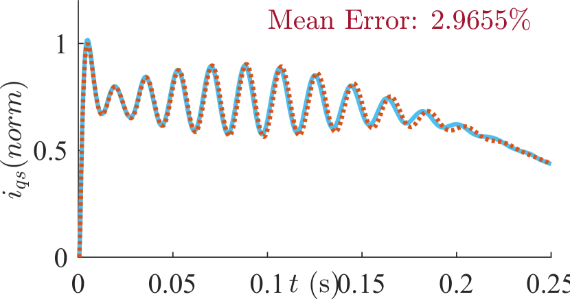
(a) prediction of G under free acceleration

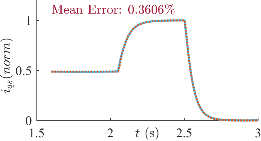
(b) prediction of G under torque change

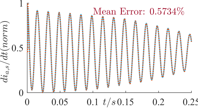
(c) prediction of P under free acceleration

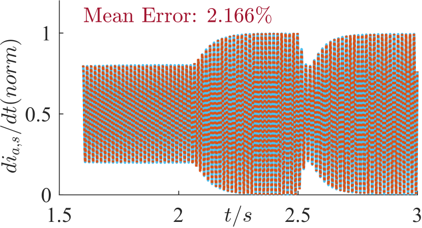
(d) prediction of P under torque change

Figure 2: Performance of NeuIM under free acceleration and torque change

As for the first fault case, the voltage starts at 2.3 kV; then at 6.01s, a three phase short circuit is applied at the terminals; later at 6.11s, the fault is cleared. In all the training set, the parameter $L_{M}$ is 0.0346 H while in the testing set of the fault case, $L_{M}$ is 0.0531 H. Fig. 3(c) illustrates the performance of the hybrid NeuIM under different portions of data. For instance, 75% hybrid means that 75% of training trajectories have the true values of the outputs of $G$, i.e. $i_{qd0s,r}$; thus the loss of these trajectories is $L_{phy}+L_{data}$. For the other 25% of the trajectories where the true values of $i_{qd0s,r}$ are unavailable, the loss of these remaining subset only consists of $L_{phy}$. The training philosophy for $P$ is always purely physics-informed.

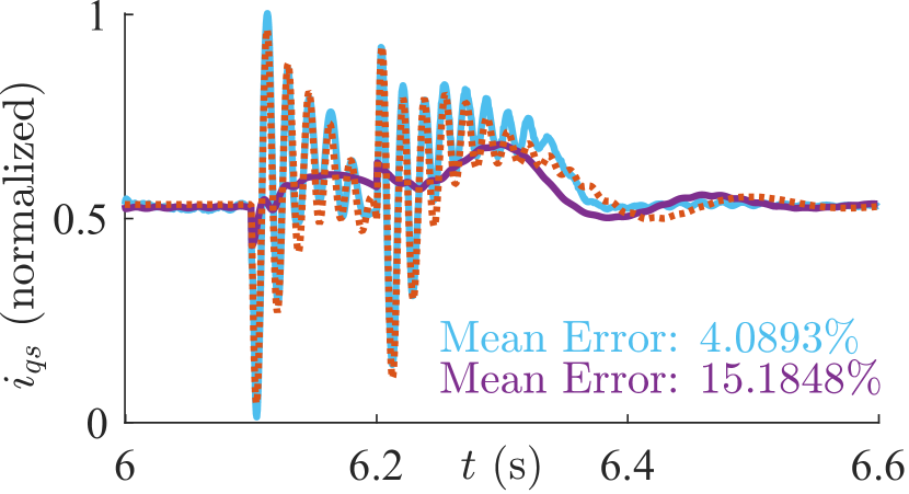
(a) Varied hybrid NeuIM performance

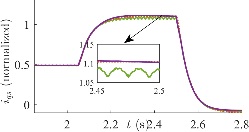
(b) purely PI NeuIM comparison

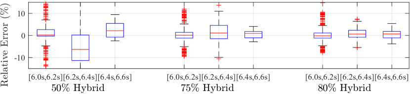
(c) Relative error comparions among varied hybrid NeuIM

Figure 3: Performance and comparions of NeuIM

From Fig. 3(c), when the proportion of data is 50%, the performance is not satisfiable. When the proportion is close to 100%, the data-driven loss takes higher weight in the total loss function. Even though the training accuracy is higher, the testing accuracy and generalization ability are compromised if it is purely data-driven. Therefore, in the next section, the optimal percentage of data, 80% data is used. Fig. 3(a) shows the 80% NeuIM performances beats pure NeuIM.

IV-B Comparison with data-driven approach

In Fig. 3(b), it is observable that the purely data-driven deep neural network (DNN), which has the same structure as NeuIM, has irregular oscillations due to its training with limited data. Meanwhile, NeuIM is not impacted by this issue.

TABLE III: MSE comparsion

Type	Fault	Torque change
Purely data-driven	0.0386	0.4330
Purely PI NeuIM	0.7352	0.0182
80% Hybrid NeuIM	0.0142	0.0158

Table III shows the final results from $P$. Hybrid physics-informed NeuIM overshadows the purely data-driven DNN in terms of accuracy, which reveals that under the same training set, NeuIM has better generalization ability to cope with unseen cases and varied parameters. For slow transients such as torque change, both NeuIM and hybrid NeuIM beat the data-driven approach. For the fault cases, the hybrid NeuIM outperforms both the data-driven method and the purely physical-informed NeuIM in terms of better convergence rates and lower MSE. The data-driven approach, even though it outperforms the pure NeuIM when data is available, it cannot grasp the transients completely when one machine parameter changed. In addition, as in Table IV, by checking the overall calculation time, NeuIM is significantly more efficient and its scalablity is guaranteed.

TABLE IV: Computation time of VBR ($\Delta t=0.5ms$) and NeuIM

Scenario	NeuIM	VBR
Free Acceleration ($T=1s$)	0.1684$s$	0.4756$s$
Torque change ($T=3.5s$)	0.5514$s$	1.2751$s$
Fault ($T=10s$)	0.5553$s$ (80% hybrid)	2.0727$s$

V Conclusion

This communication devises physics-informed Neural Induction Machine Modelling (NeuIM) and its variant hybrid NeuIM. Case studies for NeuIM and hybrid NeuIM show the efficacy of the new methods under various contingencies, and their superiority over existing purely data-driven methods. The success of NeuIM is the first step to develop an AI-driven grid simulator that replaces conventional model-based simulators.

References

- [1] H. W. Dommel, EMTP Theory Book. BPA, 1996.
- [2] P. Zhang, J. R. Marti, and H. W. Dommel, “Induction machine modeling based on shifted frequency analysis,” IEEE Transactions on Power Systems, vol. 24, no. 1, pp. 157–164, 2009.
- [3] G. E. Karniadakis, I. G. Kevrekidis, L. Lu, P. Perdikaris, S. Wang, and L. Yang, “Physics-informed machine learning,” Nature Reviews Physics, vol. 3, no. 6, pp. 422–440, 2021.
- [4] N. Amiri, S. Ebrahimi, and J. Jatskevich, “Saturable voltage-behind-reactance models of induction machines including air-gap flux harmonics,” IEEE Transactions on Energy Conversion, accepted, 2023.
- [5] L. Wang, J. Jatskevich, and S. D. Pekarek, “Modeling of induction machines using a voltage-behind-reactance formulation,” IEEE Transactions on Energy Conversion, vol. 23, no. 2, pp. 382–392, 2008.
- [6] M. Raissi, P. Perdikaris, and G. E. Karniadakis, “Physics-informed neural networks: A deep learning framework for solving forward and inverse problems involving nonlinear partial differential equations,” Journal of Computational Physics, vol. 378, pp. 686–707, Feb. 2019.
- [7] B. Huang and J. Wang, “Applications of physics-informed neural networks in power systems - a review,” IEEE Transactions on Power Systems, vol. 38, no. 1, pp. 572–588, 2023.