Abstract:  We address symmetry breaking bifurcations (SBBs) in the ground-state (GS) and dipole-mode (DM) solitons of the 1D linearly coupled NLS equations, modeling the propagation of light in a dual-core planar waveguide with the Kerr nonlinearity and two types of $\mathcal{PT}$-symmetric potentials. The ${\cal PT}$-symmetric potential is employed to obtained different types of solutions. A supercritical pitchfork bifurcation occurs in families of symmetric solutions of both the GS and DM types. A novel feature of the system is interplay between breakings of the $\mathcal{PT}$ and inter-core symmetries. Stability of symmetric GS and DM modes and their asymmetric counterparts, produced by SBBs of both types, is explored via the linear-stability analysis and simulations. It is found that the instability of $\mathcal{PT}$-symmetric solutions takes place prior to the inter-core symmetry breaking. Surprisingly, stable inter-core-symmetric GS solutions may remain stable while the $\mathcal{PT}$ symmetry is broken. Fully asymmetric GS and DM solitons are only partially stable. Moreover, we construct symmetric and asymmetric GS solitons under the action of a pure imaginary localized potential, for which the SBB is subcritical. These results exhibit that stable solitons can still be found in dissipative systems. Finally, excitations of symmetric and asymmetric GS solitons are investigated by making the potential’s parameters or the system’s coupling constant functions, showing that GS solitons can be converted from an asymmetric shape onto a symmetric one under certain conditions. These results may pave the way for the study of linear and nonlinear phenomena in a dual-core planar waveguide with $\mathcal{PT}$ potential and related experimental designs.

1 Introduction

A commonly known principle of classical and quantum physics is that the ground state (GS) of linear systems exactly follows the symmetry of the underlying Hamiltonian, while excited states may realize other representations of the same symmetry. In particular, the quantum-mechanical GS in a symmetric potential well is always spatially even, while the first excited state is represented an odd wave function [1]. The same is true for the linear propagation of light in waveguides, in which an effective potential is induced by a spatial profile of the local refractive index, as the paraxial transmission of light in the waveguide is governed by the linear equation which has the same form as the linear Schrödinger equation in quantum mechanics [2].

In nonlinear optical waveguides made of a self-focusing material, the wave propagation obeys the symmetry of the effective guiding potential only in the regime of weak nonlinearity, which is quantified by small values of the power of the optical beam. A generic effect which follows the increase of the power is the symmetry-breaking bifurcation (SBB), which makes the shape of the respective GS wave mode spatially asymmetric [3]. In particular, because the SBB gives rise to a degenerate pair of two GSs, which are mirror copies of each other, the transition to the asymmetric GS implies that the fundamental principle of quantum mechanics, which does not allow degeneracy of the GS [1], is no longer valid for nonlinear modes. Above the SBB point, a spatially symmetric mode coexists with the asymmetric GSs, but it is unstable against symmetry-breaking perturbations.

An essential ramification of the phenomenology of the spontaneous symmetry breaking is provided by SBB in dual-core waveguides, such as twin-core optical fibers, with the cubic self-focusing acting in each core [4, 5]:

$$\begin{split}i\phi_{z}&=-\frac{1}{2}\phi_{xx}-|\phi|^{2}\phi+U(x)\phi-\kappa\psi,\\ i\psi_{z}&=-\frac{1}{2}\psi_{xx}-|\psi|^{2}\psi+U(x)\psi-\kappa\phi,\end{split}$$ (1)

where $\phi\equiv\phi(x,z)$ and $\psi\equiv\psi(x,z)$ are slowly varying amplitudes of the electromagnetic waves with the transverse coordinate $x$ and propagation distance $z$, $U(x)$ represents the real-valued external potential well (e.g., $U(x)=x^{2}/2$), $\kappa$ is the linear-coupling constant. In these systems, the interplay between the intra-core self-focusing ($-|\phi|^{2}\phi$ or $-|\psi|^{2}\psi$) and group-velocity dispersion ($-\frac{1}{2}\phi_{xx}$ or $-\frac{1}{2}\psi_{xx}$), and the inter-core linear coupling ($-\kappa\psi$ or $-\kappa\phi$), provided by tunneling of light across the barrier separating the guiding core, gives rise to the inter-core SBB. The bifurcation replaces the original GS, which was symmetric with respect to the parallel cores, by a spontaneously established asymmetric one with unequal powers carried by the cores. The SBB of this type was studied in detail theoretically [6, 7, 8, 9, 10, 11] and recently demonstrated experimentally in a twin-core optical fiber (coupler) [12]. For example, symmetric and asymmetric soliton states in twin-core nonlinear optical fibers were examined using an improved variational approximation [11]. Depending on the wave form, which may be delocalized or self-trapped, the SBB in the dual-core system may be of the supercritical (forward) or subcritical (backward) type, according to the usual definition [13]. In either case, the bifurcation give rise to the destabilization of the state which is symmetric with respect to the parallel cores and creation of a pair of asymmetric ones. The SBBs of the sub- and supercritical types give rise, respectively, to branches of the asymmetric solutions which evolve backward or forward, as stable or unstable ones, with respect to the variation of the full power of the optical beam. In the subcritical case, the unstable branches reach turning points and revert to the forward direction, getting stable as a result of the reversion. Thus, the respective stable asymmetric states emerge subcritically, at a value of the power which corresponds to the turning points, being smaller than the power corresponding to the SBB point. Accordingly, the full set of stationary states is bistable in the interval between the turning and SBB points, where the stable asymmetric states coexist with the symmetric ones, which still remain stable in this interval. Furthermore, the relationships between dispersion effects and soliton dynamics were also discussed [14, 15, 16, 17] such that some soliton solutions of coupled NLS equations [14], and the modulation instability was found in nonlinear optical fibers  higher-order dispersions [17].

Symmetry-breaking effects were also studied in dual-core laser fibers, which include gain and loss in addition to the intra-core group-velocity dispersion and self-focusing nonlinearity, and inter-core linear coupling. The model of the dual-core fiber is based on a pair of linearly coupled complex Ginzburg-Landau equations [18]. A spontaneously established asymmetric regime of the operation of coupled lasers was observed in the experiment [19]. The model of the dual-core fiber including the gain and loss suggests one a possibility to consider a symmetric system with a parity-time ($\mathcal{PT}$)-symmetric distribution of spatially separated local gain and loss in each core. As is well known, linear spectra of the $\mathcal{PT}$-symmetric systems remain purely real due to the exact balance between the gain and loss, provided that the strength of the gain-loss distribution does not exceed a certain critical value [20, 21, 22, 23, 24, 25, 26, 27]. And a multitude of intensive research results on ${\cal PT}$-symmetric systems have been reported [28, 29, 30, 31, 32, 33, 34, 35, 36, 37, 38, 39, 40, 41, 42, 43]. Experimentally, setups demonstrating persistent $\mathcal{PT}$ symmetry were realized in optics [23, 44, 45].

Previously, $\mathcal{PT}$-symmetric dual-core systems were considered with the gain and loss of equal strengths carried by the different cores [46, 47]. In that system, the breakup of the $\mathcal{PT}$ symmetry, i.e., a transition from a purely real spectrum to one including complex eigenvalues, takes place when the strength of the gain and loss becomes equal to the constant of the inter-core coupling. In fact, the separation of the gain and loss between the two cores breaks the exact symmetry between them, even if the $\mathcal{PT}$ symmetry stays unbroken.

In the present work, we aim to elaborate a $\mathcal{PT}$-symmetric dual-core system of a different type, which keeps the full symmetry between the cores, each carrying the self-focusing cubic nonlinearity and a $\mathcal{PT}$-symmetric potential, i.e., a complex one whose real and imaginary parts are spatially even and odd, respectively. The main contributions of this paper can be concluded as follows:

• We introduce a model, based on the linearly-coupled NLS equations, each including the complex potential, and consider the potentials with two different imaginary parts, viz., spatially localized or delocalized ones. To the best of our knowledge, models of this type were not studied previously.

• We discuss the interplay between the nonlinearity-induced spontaneous breaking of the inter-core symmetry and breakup of the $\mathcal{PT}$ symmetry in individual cores, and numerically find that SBBs of the pitchfork type account for the breaking of the inter-core symmetry in the spatially even GS solutions and in odd ones which represent dipole modes (DMs, i.e., the first excited states admitted by the intra-core potentials).

• Unlike the even GS soliton, dipole mode does not exist in the absence of the harmonic-oscillator potential. And as the strength of gain and loss changes, the solitons exhibit different states. The breakup of the $\mathcal{PT}$ symmetry occurs before the breaking of the inter-core symmetry. A noteworthy finding is that stable inter-core-symmetric GS solutions keep their stability in a small region even when the $\mathcal{PT}$ symmetry is broken.

• An essential difference from the well-known properties of the nonlinear coupler without the gain and loss terms is that inter-core asymmetric GS and DM modes are only partly stable, as some of them are destabilizes by the $\mathcal{PT}$-symmetry breaking.

• For the system with purely imaginary potentials, the SBB changes its character from supercritical to subcritical.

• We investigate the transforms between symmetric and asymmetric GS modes in a nonstationary system, in which parameters of the $\mathcal{PT}$-symmetric potential and/or the inter-core coupling constant are defined as functions of the propagation distance. In particular, it is found that asymmetric GS modes can be transformed back into symmetric ones by means of a properly defined modulation.

The rest of this paper is arranged as follows. Sec. 2 introduces a model, based on the linearly-coupled NLS equations, each including the complex potential with two different imaginary parts, viz., spatially localized or delocalized ones. In Sec. 3, we mainly discuss the interplay between the nonlinearity-induced spontaneous breaking of the inter-core symmetry and breakup of the $\mathcal{PT}$ symmetry in individual cores. In Sec. 4, we address the SSB in the system with purely imaginary potentials (without the real part). In Sec. 5, transformations between symmetric and asymmetric GS modes are investigated in a nonstationary (modulated) system. In Sec. 6, we give the physical interpretations for all figures. And the paper is concluded and discussed by Sec. 7.

2 The dual-core system with $\mathcal{PT}$-symmetric potentials

2.1 The physical model and stationary soliton solutions

The 1D twin-core optical fibers, with the cubic self-focusing acting in each core have been studied [4, 5]. Here we consider the 1D system of linearly coupled NLS equations, modeling the propagation of light in a dual-core planar waveguide with the transverse coordinate $x$, propagation distance $z$, intra-core Kerr nonlinearity, and the $\mathcal{PT}$-symmetric potential is written as

$$\begin{split}i\phi_{z}&=-\frac{1}{2}\phi_{xx}-|\phi|^{2}\phi+\left[V(x)+iW(x)\right]\phi-\lambda\psi,\\ i\psi_{z}&=-\frac{1}{2}\psi_{xx}-|\psi|^{2}\psi+\left[V(x)+iW(x)\right]\psi-\lambda\phi,\end{split}$$ (2)

where $\phi\equiv\phi(x,z)$ and $\psi\equiv\psi(x,z)$ are slowly varying complex amplitudes of the electromagnetic waves. The complex-valued potential $V(x)+iW(x)$ is the $\mathcal{PT}$-symmetric one provided that its real and imaginary parts are, respectively, even and odd functions, i.e., $V(-x)=V(x)$ and $W(-x)=-W(x)$. In fact, the ${\cal PT}$-symmetric external potential can be realized via a judicious inclusion of loss or gain domains in guided wave geometries [23, 48]. We choose the real part as the harmonic-oscillator potential, $V(x)=\frac{1}{2}x^{2}$, which is relevant as the trap in many physical realizations, while the imaginary part with strength $W_{0}$ and intrinsic scale $l$ can be naturally chosen as the spatially delocalized one

$$W_{1}(x)=W_{0}\tanh\left(\frac{x}{l}\right),$$ (3)

or spatially localized one

$$W_{2}(x)=W_{0}\,\mathrm{sech}\left(\frac{x}{l}\right)\tanh\left(\frac{x}{l}\right).$$ (4)

Real parameter $\lambda>0$ in Eq. (2) is the inter-core coupling coefficient which couples the parallel cores. Further, we assume that the strengths of the self-focusing nonlinear terms are equal in both cores, being fixed equal to $1$ by means of rescaling. We stress that, while imaginary potential (3) does not vanish ($W_{1}(x)\rightarrow\pm W_{0}$) at $|x|\rightarrow\infty$, it may have a chance to support stable modes due to the presence of the strong confining potential $\sim x^{2}$, cf. Ref. [49].

With propagation distance $z$ replaced by time $t$, Eq. (2) plays the role of the generalized Gross-Pitaevskii (GP) equation for Bose-Einstein condensates (BECs) loaded in the $\mathcal{PT}$-symmetric potential [50, 27]. Furthermore, Eq. (2) can be rewritten in the variational form $i\{\phi,\psi\}_{z}=\delta H/(\delta\{\phi^{\ast},\psi^{\ast}\})$ with the generalized complex-values Hamiltonian:

$$H=\int_{-\infty}^{+\infty}\Big{[}\frac{1}{2}(|\phi_{x}|^{2}+|\psi_{x}|^{2})-\frac{1}{2}(|\phi|^{4}+|\psi|^{4})+(V(x)+iW(x))(|\phi|^{2}+|\psi|^{2})-\lambda(\phi^{\ast}\psi+\phi\psi^{\ast})\Big{]}\mathrm{d}x,$$ (5)

where $\ast$ represents the complex conjugate.

Solutions produced by Eq. (2) are characterized by their total optical power (in the application to BECs, it is the total norm),

$$P(z)=P_{1}(z)+P_{2}(z)\equiv\int_{-\infty}^{+\infty}|\phi(x,z)|^{2}dx+\int_{-\infty}^{+\infty}|\psi(x,z)|^{2}dx.$$ (6)

It follows from Eq. (2) that the evolution equation for the power is

$$\frac{dP(z)}{dz}=-2\int_{\mathbb{R}}W(x)(|\phi|^{2}+|\psi|^{2})dx.$$ (7)

Note that the power is conserved for solutions in which local powers $|\phi(x)|^{2}$ and $|\psi(x)|^{2}$ are even functions of $x$, as the imaginary part $W(x)$ of the complex potential is an odd function, due to the condition of the $\mathcal{PT}$ symmetry.

Stationary solutions of Eq. (2) are looked for in the usual form,

$$\left\{\phi(x,z),\psi(x,z)\right\}=\left\{u(x),v(x)\right\}e^{-i\mu z},$$ (8)

where real $-\mu$ stands for the propagation constant ($\mu$ is the chemical potential in the GP version of the model), and stationary wave functions $\left\{u(x),v(x)\right\}$ vanish at $x\rightarrow\pm\infty$. Substituting ansatz (8) in Eq. (2) yields the following coupled ordinary differential equations:

$$\begin{split}\mu u=&-\frac{1}{2}\frac{d^{2}u}{dx^{2}}-|u|^{2}u+(V(x)+iW(x))u-\lambda v,\\ \mu v=&-\frac{1}{2}\frac{d^{2}v}{dx^{2}}-|v|^{2}v+(V(x)+iW(x))v-\lambda u.\end{split}$$ (9)

Symmetric and antisymmetric solutions, with $u=v$ or $u=-v$, respectively, obey the single equation

$$\left(\mu\pm\lambda\right)u=-\frac{1}{2}\frac{d^{2}u}{dx^{2}}-|u|^{2}u+(V(x)+iW(x))u.$$ (10)

The Lagrangian corresponding to Eq. (9) is shown as follows

$$\begin{split}\displaystyle L=&\int_{\mathbb{R}}\left[\frac{1}{2}(|u_{x}|^{2}+|v_{x}|^{2})-\frac{1}{2}(|u|^{4}+|v|^{4})+(V(x)+iW(x))(|u|^{2}+|v|^{2})-\lambda(u^{*}v+uv^{*})\right.\\ &\left.\qquad-\mu(|u|^{2}+|v|^{2})\right]\mathrm{d}x.\end{split}$$ (11)

Notice that the stationary solutions (8) can be studied analytically in terms of the variational approximation related to Eq. (11) [51], and numerically via the modified squared-operator iteration method [52, 53]. Furthermore, if one desires to investigate the temporal progression of approximate wave functions characterized by generalized time-dependent collective coordinates in the presence of a complex potential, then the dissipation functional formalism was commonly employed [54]. In a specific case involving a ${\cal PT}$-symmetric potential, the evolution of the collective coordinates was examined, leading to the identification of an instability criterion for a ground state solution. Subsequently, this formalism, along with the aforementioned stability criterion, was utilized to analyze the evolution of solitons in the coupled NLS equations subject to potentials exhibiting both even and odd-${\cal PT}$ characteristics [55, 56].

Stability of stationary solutions (8) is a crucially important issue. In particular, antisymmetric states, with $u=-v$, are definitely unstable, as $\lambda>0$ implies that they have a positive, rather than negative, coupling energy.

The bifurcations breaking the symmetry between the components of the solution in the two cores takes place when total power $P$ of the symmetric state exceeds a critical value, i.e., at $P>P_{\mathrm{cr}}$. The asymmetry of states with unequal powers in the two cores, $P_{1}\neq P_{2}$, is characterized by parameter

$$\theta=\frac{|P_{1}-P_{2}|}{P_{1}+P_{2}}.$$ (12)

On the other hand, the breaking of the $\mathcal{PT}$ symmetry occurs when strength $W_{0}$ of gain-loss distribution, represented by the imaginary potential $W(x)$, attains a certain threshold value. A problem relevant to the system under the consideration, which was not addressed in previous works, is to find $P_{\mathrm{cr}}$ as functions of $W_{0}$.

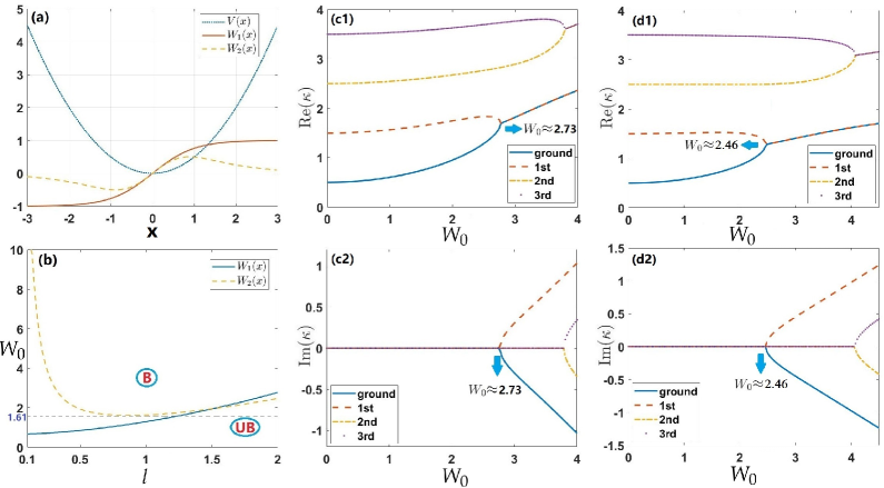
Figure 1: $\mathcal{PT}$ symmetry breaking for the linear spectral problem (13) with differential gain-and-loss distributions given by Eqs. (3) and (4). (a) Profiles of real and imaginary parts of the $\mathcal{PT}$-symmetric potentials (3) and (4) at $W_{0}=l=1$. (b) Results of the solution of the linear spectral problem (13) for potentials $W_{1}(x)$ and $W_{2}(x)$, where “UB” (“B”) denotes the area of the unbroken (broken) $\mathcal{PT}$ symmetry below (above) the breaking lines, respectively. (c1,c2) Real and imaginary parts of the first two eigenvalues $\kappa$ as functions of $W_{0}$ at $l=2$ for $W_{1}(x)$, where the $\mathcal{PT}$ symmetry breaking occurs at $W_{0}\approx 2.73$. (d1,d2) Real and imaginary parts of the first two eigenvalues $\kappa$ as functions of $W_{0}$ at $l=2$ for $W_{2}(x)$, where the $\mathcal{PT}$ symmetry breaking occurs at $W_{0}\approx 2.46$.

2.2 The linear spectral problem and $\mathcal{PT}$-symmetry breaking

The calculation of the linear spectrum of the single equation (10) with $\lambda=0$ is a well-known basic problem in the theory of linear $\mathcal{PT}$-symmetric systems. Here, we first consider the $\mathcal{PT}$-symmetry breaking for the following linear non-Hermitian Hamiltonian related to system (9):

$$\left(\begin{array}[]{cc}\mathcal{H}&-\lambda\\ -\lambda&\mathcal{H}\end{array}\right)\left(\begin{array}[]{c}\hat{u}\\ \hat{v}\end{array}\right)=\kappa\left(\begin{array}[]{c}\hat{u}\\ \hat{v}\end{array}\right),\quad\mathcal{H}=-\frac{1}{2}\partial_{x}^{2}+\frac{1}{2}x^{2}+iW(x),$$ (13)

where $\kappa$ and $(\hat{u},\hat{v})^{T}$ are the eigenvalue and localized eigenfunction, respectively. Although $\lambda$ affects the spectrum of the linear eigenvalue problem (13), the $\mathcal{PT}$ symmetry breaking is independent of $\lambda$, i.e., $\lambda$ has no effect on the occurrence of complex eigenvalues.

The profiles of real and imaginary parts of potentials (3) and (4) for $W_{0}=l=1$ are shown in Fig. 1(a), which shows that the harmonic-oscillator potential imposes strong confinement on the wave function, even if imaginary potential (3) does not vanish at $|x|\rightarrow\infty$. Boundaries between unbroken and broken $\mathcal{PT}$ symmetry, obtained by means of the Fourier spectral method [52, 57] for imaginary potentials $W_{1}(x)$ and $W_{2}(x)$ in the $(l,W_{0})$ plane, are plotted in Fig. 1(b). The broken (unbroken) $\mathcal{PT}$-symmetry takes place above (under) the boundaries. For example, if $l=2$ is fixed, the $\mathcal{PT}$ symmetry-breaking threshold for $W_{1}(x)$ and $W_{2}(x)$ is $W_{0}\approx 2.73$ and $2.46$, respectively. To further illustrate the $\mathcal{PT}$-symmetry breaking process for $W_{1}(x)$ and $W_{2}(x)$, eigenvalues of the first four lowest energy levels are plotted as functions of $W_{0}$ for fixed $l=2$ in Figs. 1(c1,c2,d1,d2). The plots demonstrate that the $\mathcal{PT}$ symmetry gets broken at critical points, through collisions of the real eigenvalues corresponding to ground and first excited state at $W_{0}\approx 2.73$ for $W_{1}(x)$, or at $W_{0}\approx 2.46$ for $W_{2}(x)$.

2.3 The linear-stability analysis

To analyze the linear stability of stationary solutions (8), the perturbed solution of Eq. (2)

$$\begin{split}\phi(x,z)&=\left\{u(x)+\rho\left[F_{1}(x)e^{-i\varepsilon z}+G_{1}^{\ast}(x)e^{i\varepsilon^{\ast}z}\right]\right\}e^{-i\mu z},\\ \psi(x,z)&=\left\{v(x)+\rho\left[F_{2}(x)e^{-i\varepsilon z}+G_{2}^{\ast}(x)e^{i\varepsilon^{\ast}z}\right]\right\}e^{-i\mu z},\end{split}$$ (14)

are employed, where $0<\rho\ll 1$ is an infinitesimal amplitude of the perturbations, $F_{j}(x)$ and $G_{j}(x)$ $(j=1,2)$ are eigenfunctions of the linearized eigenvalue problem, and $\varepsilon$ is the respective eigenvalue. Substituting the perturbed solution (14) into the full nonlinear system of Eq. (2) and linearizing around the localized solution, we derive the corresponding Bogoliubov-de Gennes (BdG) equations [58]:

$$\left(\begin{array}[]{cccc}L_{1}&-\lambda&L_{3}&0\\ -\lambda&L_{2}&0&L_{4}\\ -L_{3}^{*}&0&-L_{1}&\lambda\\ 0&-L_{4}^{*}&\lambda&-L_{2}\\ \end{array}\right)\left(\begin{array}[]{c}F_{1}\\ F_{2}\\ G_{1}\\ G_{2}\\ \end{array}\right)=\varepsilon\left(\begin{array}[]{c}F_{1}\\ F_{2}\\ G_{1}\\ G_{2}\\ \end{array}\right),$$ (15)

$$L_{1}=-\frac{1}{2}\partial_{x}^{2}-2|u|^{2}+\frac{1}{2}x^{2}+iW(x)-\mu,\quad L_{2}=-\frac{1}{2}\partial_{x}^{2}-2|v|^{2}+\frac{1}{2}x^{2}+iW(x)-\mu,\quad L_{3}=-u^{2},\quad L_{4}=-v^{2}.$$ (16)

The stationary states are linearly unstable if at least one eigenvalue $\varepsilon$ is complex. To clearly identify the change of spectra of the above eigenvalue problem produced by the numerical solution, we set the linear-instability index

$$\tau=\log_{10}(\max\{|\mathrm{Im}(\varepsilon)|\}),$$ (17)

and categorize the underlying solution as a stable one if $\tau\leq-8$, otherwise the solution is unstable.

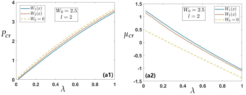
Figure 2: Boundaries of the $\mathcal{PT}$ symmetry breaking for the inter-core symmetry $P_{\mathrm{cr}}(\lambda)$ and propagation constant $-\mu_{\mathrm{cr}}$. (a1) The boundary for the breaking of the inter-core symmetry, $P_{\mathrm{cr}}(\lambda)$, for the $\mathcal{PT}$-symmetric potentials $W_{1}(x)$ and $W_{2}(x)$ at $W_{0}=2.5$ and $l=2$, respectively. (a2) Critical values of propagation constant $-\mu_{\mathrm{cr}}$ at the inter-core symmetry-breaking point of the GS modes versus the inter-core coupliing constant $\lambda$ for the potentials $W_{1}(x)$ and $W_{2}(x)$ at $W_{0}=2.5$ and $l=2$, respectively. The yellow dotted line shows the results for $W_{0}=0$, i.e., for the pure real potential.

3 Symmetry breaking of nonlinear modes and their stability

In this section, we concentrate on the SBB of nonlinear modes including ground-state and dipole modes and their stability. Especially, the influence of the imaginary part $W(x)$ of the $\mathcal{PT}$-symmetric potential on SBB is investigated. The modified squared-operator iteration method [52, 53] is used to find the numerical solutions. And based on the Fourier collocation method, the stability of these solutions is discussed by solving the BdG equations (15). Finally, the dynamics of symmetric and asymmetric modes is further studied by direct simulations of the perturbed solution.

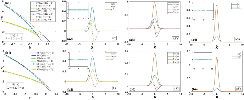
Figure 3: Total power $P$ versus propagation constant $-\mu$ for symmetric (SY) and asymmetric (ASY) GS modes. (a1) The $\mathcal{PT}$-symmetric potential is $W_{1}(x)$, with $W_{0}=2$, $l=2$ and inter-core coupling constant $\lambda=0.3$. (b1) Potential $W_{2}(x)$ with $W_{0}=1$, $l=2$, and $\lambda=0.3$, The results corresponding to the real potential (with $W_{0}=0$) are also presented. (a2,b2) Profiles of stable symmetric GS solutions $u(x)$ for $W_{1}(x)$, $\mu=0.4$, and $W_{2}(x)$, $\mu=0.1$, respectively. (a3,a4,b3,b4) Profiles of stable asymmetric GS solutions $u(x)$ and $v(x)$ for $W_{1}(x)$, $\mu=0.1$ and $W_{2}(x)$, $\mu=-0.4$, respectively. Here “uns” and “s” refer to unstable and stable solutions, respectively. The inset shows stability spectra for eigenvalues $\varepsilon$ of small perturbations, see Eq. (14).

3.1 Symmetric and asymmetric ground-state (GS) modes

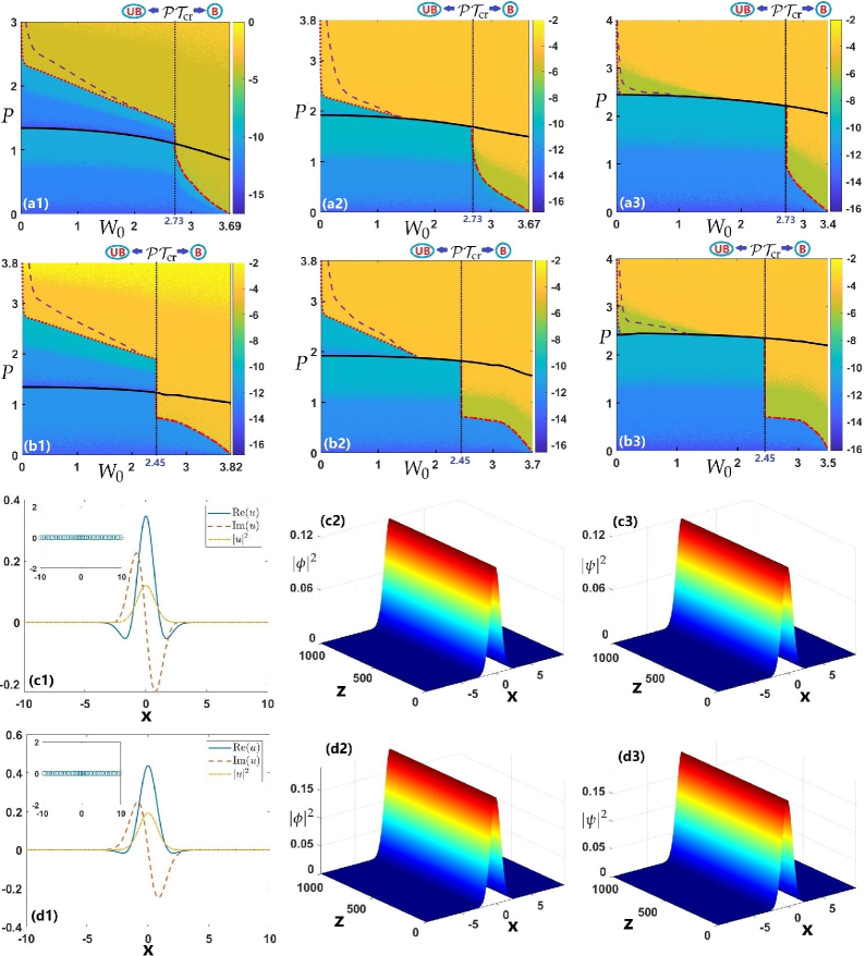
Figure 4: The stability and boundary of the breaking of the inter-core symmetry for symmetric and asymmetric GS modes in $(W_{0},P)$-space with $l=2$. The colorbar denotes the linear instability index $\tau$ defined in Eq. (17). Panels (a1,a2,a3) correspond to symmetric and asymmetric GS modes for the $\mathcal{PT}$-symmetric potential $W_{1}(x)$ and inter-core coupling constants $\lambda=0.3$, $0.45$ and $0.6$, respectively. Panels (b1,b2,b3) correspond to symmetric and asymmetric GS modes for $W_{2}(x)$ and $\lambda=0.3$, $0.45$ and $0.6$, respectively. Here the black solid line represents the boundary for the breaking of the inter-core symmetry, $P_{\mathrm{cr}}(W_{0})$. Regions below and above the black line represent, respectively, symmetric (SY) solutions and asymmetric ones (ASY). The red dotted line represents the instability boundary of symmetric solutions (asymmetric solutions) below (above) the black line. The yellow instability area of asymmetric solutions above the purple dotted line represents the instability (collapse) shown in Fig. 6(b1-b4), while the oscillating instability displayed in Fig. 6(c1-c4) takes place in the yellow area below the purple dotted line. The vertical dotted line indicates the $\mathcal{PT}$-symmetry breaking point ($\mathcal{PT}_{\mathrm{cr}}\approx 2.73$ for potential $W_{1}(x)$, and $\mathcal{PT}_{\mathrm{cr}}\approx 2.45$ for $W_{2}(x)$), where “UB” (“B”) denotes the phases with unbroken (broken) $\mathcal{PT}$ symmetry. (c1,c2,c3) Profiles of stable symmetric GS solutions $u(x)$ for $\lambda=0.3$ and $W_{1}(x)$ with $W_{0}=2.8$, $l=2$ ($\mathcal{PT}$ breaking) and $\mu=1$ ($P\approx 0.437$), and the corresponding numerically simulated evolution. (d1,d2,d3) Profiles of stable symmetric GS solutions $u(x)$ for $\lambda=0.3$ and $W_{2}(x)$ with $W_{0}=2.5$, $l=2$ ($\mathcal{PT}$ breaking) and $\mu=0.6$ ($P\approx 0.7109$) and the corresponding numerically simulated evolution.

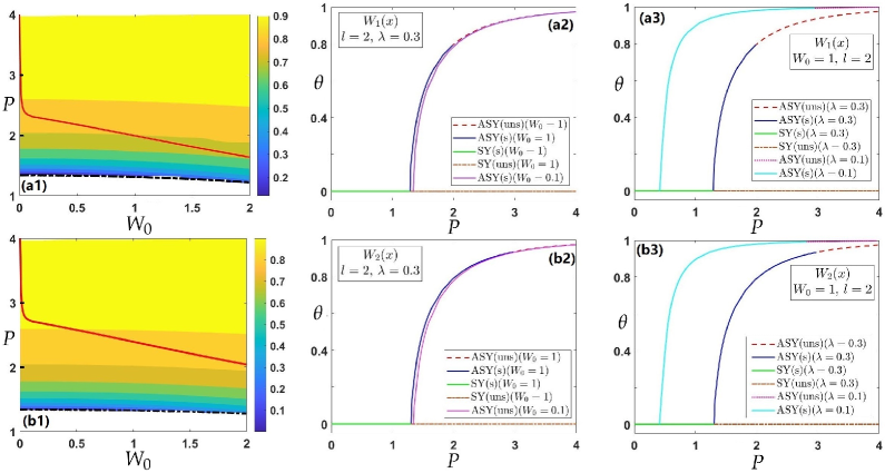
Figure 5: (a1,b1) Asymmetry characteristic $\theta$ (see Eq. (12)) in $(W_{0},P)$-space for the $\mathcal{PT}$-symmetric potentials $W_{1}(x)$ and $W_{2}(x)$ with $l=2$, respectively, and $\lambda=0.3$. Here the red line is the stability boundary for the asymmetric states. Bifurcation diagrams in the $(P,\theta)$ plane for the GS modes with different parameters: (a2,b2) the bifurcation diagrams for potentials $W_{1}(x)$ and $W_{2}(x)$ with $l=2$ and $\lambda=0.3$; (a3,b3) the bifurcation diagrams for $W_{1}(x)$ and $W_{2}(x)$ with $W_{0}=1$ and $l=2$. Here “ASY(uns)” and “ASY(s)” represent unstable and stable asymmetric solutions, respectively, while “SY(uns)” and “SY(s)” represent unstable and stable symmetric solutions.

At first, for GS solutions, the boundary for the breaking of the inter-core symmetry $P_{\mathrm{cr}}(\lambda)$ can be obtained for the imaginary potentials $W_{1}(x)$ and $W_{2}(x)$ at fixed potential parameters, viz., $W_{0}=2.5$ and $l=2$, see Fig. 2(a1). For a fixed coupling constant $\lambda$, when the total power $P$ exceeds the threshold $P_{\mathrm{cr}}$, the symmetry breaking occurs and asymmetric solutions appear. With the increase of $\lambda$, larger values of power $P$ are naturally required for the occurrence of the symmetry breaking. The power required for symmetry breaking under the action of potential $W_{2}(x)$ is slightly larger than that required in the case of $W_{1}(x)$. Meanwhile, when $W_{0}=0$ (i.e., the potential is real), the boundary for the breaking of the inter-core symmetry is also exhibited in Fig. 2(a1). By comparison, we see that a larger gain-loss strength reduces the power needed for the symmetry breaking, but not significantly. Furthermore, Fig. 2(a2) displays the critical values of propagation constant $-\mu_{\mathrm{cr}}$ at the symmetry-breaking point of the GS modes for imaginary potentials $W_{1}(x)$ and $W_{2}(x)$, respectively. According to the results obtained for the real potential (see the yellow dotted line in Fig. 2(a2)), the effect of the imaginary part $W(x)$ of the potential on the relation between the propagation constant $-\mu$ and power $P$ is obvious.

To clearly display the relation between $\mu$ and $P$, the results for the symmetric and asymmetric GS modes are presented by means of $P(\mu)$ dependences for potential $W_{1}(x)$ at $W_{0}=2$ and $W_{2}(x)$ at $W_{0}=1$ in Figs. 3(a1,b1), respectively. The results for the real potential, with $W_{0}=0$, are also exhibited for the comparison. It is seen that, with the increase of power $P$, the curves for the real and complex $\mathcal{PT}$-symmetric potentials gradually coalesce. Note that all the results satisfy the Vakhitov-Kolokolov (VK) criterion ($\mathrm{d}P/\mathrm{d}\mu<0$), which is the necessary condition for stability of solutions in the case of any self-focusing nonlinearity (see the original work [59] and detailed explanations in Refs. [60, 61, 62]). However, the asymmetric GS modes are only partially stable. For instance, for potential $W_{1}(x)$ with $W_{0}=2$ and $l=2$, the asymmetric GS becomes unstable at $P>1.5878$. This is in contrast with the case of the real potential, in which case the asymmetric GS is always stable when it exists [5]. In the limit of $\mu\rightarrow-\infty$, the small component of an asymmetric solution is $v(x)\approx-(\lambda/\mu)u(x)$ according to Eq. (9). Therefore, for fixed coupling constant $\lambda$, $P_{2}=\int_{-\infty}^{+\infty}|\psi(x,z)|^{2}dx\rightarrow 0$ as $\mu\rightarrow-\infty$. Thus, in the limit of $\mu\rightarrow-\infty$, the total powers of the symmetric and asymmetric solutions are related so that

$$P_{\mathrm{sym}}\approx 2P_{\mathrm{asym}}.$$ (18)

In Figs. 3(a2-a4,b2-b4), some typical examples of the stable symmetric and asymmetric GS solutions for imaginary potentials $W_{1}(x)$ and $W_{2}(x)$ are exhibited.

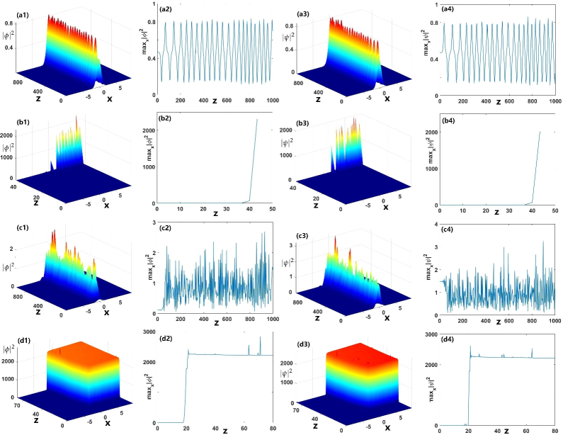
Figure 6: The numerically simulated evolution of an unstable GS state and the respective evolution of maximum densities of the components in the parallel cores for the $\mathcal{PT}$-symmetric potential $W_{1}(x)$ and inter-core coupling constant $\lambda=0.3$. (a1-a4) A symmetric GS solution for $W_{0}=1$ and $l=2$ at $\mu=-0.045$ ($P\approx 1.5$), which shows the oscillatory instability. (b1-b4) A symmetric GS solution for $W_{0}=2.8$ and $l=2$ at $\mu=0.75$ ($P\approx 0.9$), which shows the collapse of the soliton. (c1-c4) An asymmetric GS solution with $W_{0}=1$ and $l=2$ at $\mu=-0.5$ ($P\approx 2.14$), which shows the oscillatory instability. (d1-d4) An asymmetric GS solution with $W_{0}=2.8$ and $l=2$ at $\mu=0.4$ ($P\approx 1.32$), which shows the collapse.

Note that, for the GS modes, the results produced by the imaginary potentials $W_{1}(x)$ and $W_{2}(x)$ are similar when their amplitude $W_{0}$ is small. However, when the strength of gain-loss distribution is large, the corresponding results for the SBB and stability are different. Figure 4 exhibits the stability and boundary of the breaking of the inter-core symmetry for symmetric and asymmetric GS modes in the plane of $(W_{0},P)$. It is observed that the imaginary part $W(x)$ of the potential produces an effect on the breaking of the inter-core symmetry and stability. With the increase of $W_{0}$, the critical values of the power at symmetry-breaking point gradually decrease. Furthermore, for conservative systems the boundary of the inter-core symmetry breaking is, generally, a boundary of destabilization of the symmetric GS modes. However, near the $\mathcal{PT}$-symmetry breaking point, the stability of the symmetric solution becomes unstable at smaller $P$. For example, for the potential $W_{1}(x)$ with $l=2$, the $\mathcal{PT}$-symmetric breaking occurs at $W_{0}>2.73$, according to Fig. 1(b), which leads to the onset of instability of symmetric solutions before the inter-core symmetry breaking occurs (see Figs. 4(a1,a2,a3) corresponding to $\lambda=0.3,0.45$ and $0.6$, respectively). On the other hand, an important finding is that there still exist stable symmetric solutions in the region of the broken $\mathcal{PT}$ symmetry. For example, for the potential $W_{1}(x)$ with $W_{0}=2.8$ and $l=2$, stable symmetric solutions can be found at $P\approx 0.437$ and $\lambda=0.3$ as is shown in Figs. 4(c1,c2,c3). For the potential $W_{2}(x)$ with $W_{0}=2.5$ and $l=2$, stable symmetric solutions are obtained at $P\approx 0.7109$ and $\lambda=0.3$, see Figs. 4(d1,d2,d3). When $W_{0}=0$, i.e., the potential is real, the asymmetric GS modes, are always stable. However, when the imaginary part $W(x)$ of the potential is added, the asymmetric solutions becomes unstable when power $P$ exceeds a certain threshold, as shown by the red dotted line above the black line in Fig. 4. As $W_{0}$ increases, the stability region of the asymmetric solution shrinks. Eventually, there is no stable asymmetric solution after the $\mathcal{PT}$-symmetry breaking occurs. When the inter-core coupling constant $\lambda$ is larger, the critical power at the point of the breaking of the inter-core symmetry is larger too. As $\lambda$ increases, the stability region of the asymmetric solutions shrinks. For example, there is a conspicuous stability region for the asymmetric states at $\lambda=0.45$, which almost disappears at $\lambda=0.6$, see Figs. 4(a3,b3).

The SBB of the GS modes is illustrated by heatmaps of asymmetry parameter $\theta$, see Eq. (12), in the plane of $(W_{0},P)$ for imaginary potentials $W_{1}(x)$ and $W_{2}(x)$ with $\lambda=0.3$ and $l=2$ in Figs. 5(a1,b1). The bifurcation diagrams are also exhibited in Figs. 5(a2,a3,b2,b3) by means of $\theta(P)$ curves for fixed parameters of the system. These diagrams clearly demonstrate that the SBB for the GS modes is of the supercritical type, i.e., the emerging branches of the asymmetric solutions go forward (rather than backward) as the power keeps growing past the SBB point, according to the usual definition [13]. On the other hand, strength $W_{0}$ of the gain-loss distribution has a little effect on $\theta$, while it affects the stability of the solutions. It is also worthy to note that the stability region is much larger for the $\mathcal{PT}$ potential $W_{2}(x)$ than for $W_{1}(x)$.

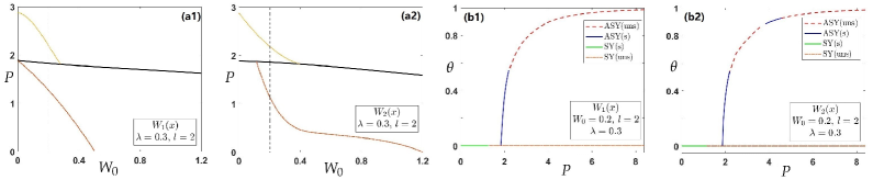
Figure 7: The stability and the boundary of the breaking of the inter-core symmetry for symmetric and asymmetric DM modes in $(W_{0},P)$-space with $\lambda=0.3$, $l=2$ and imaginary potentials $W_{1}(x)$ in (a1) and $W_{2}(x)$ in (a2). Here the black solid line represents the boundary of the breaking of the inter-core symmetry. The regions below and above the black line are populated, respectively, by the symmetric (SY) and asymmetric (ASY) DM solutions. The red (yellow) dotted line represents the instability boundary of symmetric (asymmetric) solutions below (above) the black line. The region below the dotted line represents stable solutions. (b1,b2) Bifurcation diagrams in the $(P,\theta)$ plane for imaginary potentials $W_{1}(x)$ and $W_{2}(x)$ with $W_{0}=0.2$, $l=2$ and $\lambda=0.3$. Here “ASY(uns)” and “ASY(s)” represent unstable and stable asymmetric solutions, respectively. “SY(uns)” and “SY(s)” represent unstable and stable symmetric solutions, respectively.

3.2 Dynamics of symmetric and asymmetric ground-state (GS) modes

Figure 6 shows the numerically simulated evolution of unstable GS states, to which random perturbation are added at the 2% amplitude level, in the case of the $\mathcal{PT}$-symmetric potential $W_{1}(x)$ and inter-core coupling constant $\lambda=0.3$. For symmetric GS modes, the SBB causes oscillatory instability, see Figs. 6(a1-a4). In the simulations, the symmetric state spontaneously transforms into an asymmetric one with residual oscillations. Figures 6(a2, a4) demonstrate that minimum and maximum amplitudes of both components are attained at the same time. However, in the $\mathcal{PT}$-broken region the symmetric GS is collapses (see Figs. 6(b1-b4)), where the amplitude of the imaginary part of the potential is $W_{0}=2.8$.

Asymmetric GS modes become unstable when their power $P$ exceeds a certain threshold value, as shown in Fig. 4. At first, the asymmetric solutions exhibit oscillating instability (see Figs. 6(c1-c4)), which is followed by the onset of collapse with the increase of $P$. The corresponding instability boundary is displayed by the purple dotted line in Fig. 4. The yellow instability area of asymmetric solutions above the purple dotted line represents the collapse, while the oscillatory instability takes place in the yellow area below the purple dotted line. Simultaneously, due to the presence of $\mathcal{PT}$-symmetry breaking, the asymmetric GS solutions start to collapse.

3.3 Symmetric and asymmetric dipole modes (DM) and their dynamics

Similarly, systematic results for symmetric and asymmetric DMs (first excited states) have been collected too. First, the critical values of power $P_{\mathrm{cr}}(W_{0})$ (the black solid line) at the symmetry-breaking point for the imaginary potentials $W_{1}(x)$ and $W_{2}(x)$, respectively, are exhibited in Figs. 7(a1) and (a2). At $P>P_{\mathrm{cr}}$, the inter-core symmetry breaking occurs and symmetric DMs appear. Compared to the GS modes, the critical value of the power is somewhat higher for the dipoles than for the GS modes, cf. Figs. 7(a1,a2) and Figs. 4(a1,b1). This happens because the shape of the dipoles is broader than that of GS modes, which makes the nonlinearity weaker for the dipoles, in comparison with the GS mode. Besides, the stable region of symmetric DMs shrinks rapidly as $W_{0}$ increases, especially for the $W_{1}(x)$ potential, and this instability penetrates into a part of the originally stable branches of the symmetric DMs below the SBB point, as shown in Figs. 7(a1,a2), where the red dotted line represents the instability boundary of symmetric solutions below the black line.

Fixing $W_{0}=0.2$, $l=2$ and $\lambda=0.3$, the bifurcation diagrams in the $(P,\theta)$ plane for imaginary potentials $W_{1}(x)$ and $W_{2}(x)$ are shown, severally, in Figs. 7(b1) and (b2). The diagrams clearly demonstrate that the SBB for the DMs is of the supercritical type. Under the action of the imaginary part of the potential, asymmetric DMs feature partial stability, with respective complex instability eigenvalues. The instability boundary of asymmetric solutions is displayed by yellow dotted line in Figs. 7(a1,a2).

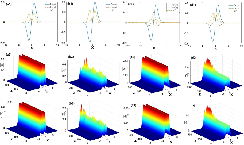
Figure 8: Profiles of stable and unstable symmetric DM solutions $u(x)$ at $\lambda=0.3$ for imaginary potentials $W_{1}(x)$ and $W_{2}(x)$ with $l=2$, and the corresponding numerically simulated evolution. Panels (a1,a2,a3) display stable DM solutions for $W_{1}(x)$ with $W_{0}=0.2$ at $\mu=1.05$ ($P\approx 1.0012$). Panels (b1,b2, b3) display unstable DM solutions for $W_{1}(x)$ with $W_{0}=0.2$ at $\mu=0.95$ ($P\approx 1.6399$). Panels (c1,c2,c3) display stable DM solutions for $W_{2}(x)$ with $W_{0}=1$ at $\mu=1.1$ ($P\approx 0.165$). Panels (d1,d2,d3) display unstable DM solutions for $W_{2}(x)$ with $W_{0}=1$ at $\mu=0.98$ ($P\approx 1.5158$).

Figures 8 and 9 display profiles of symmetric and asymmetric DM solutions, as well as the corresponding numerically simulated evolution with random noise at the 2% amplitude level. In general, when the strength of the gain-loss distribution is weak, the DM solutions exhibit oscillatory instability, as shown in the Figs. 8(b2,b3). However, at larger $W_{0}$ the DMs tend to collapse, see Figs. 8(d2,d3).

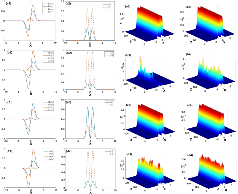
Figure 9: Profiles of stable and unstable asymmetric DM solutions $u(x)$ and $v(x)$ at $\lambda=0.3$ for imaginary potentials $W_{1}(x)$ and $W_{2}(x)$ with $W_{0}=0.2$ and $l=2$, and the corresponding numerically simulated evolution. (a1-a4): Stable DM solutions for $W_{1}(x)$ at $\mu=0.85$ ($P\approx 2.0577$). (b1-b4): Unstable DM solutions for $W_{1}(x)$ at $\mu=0.7$ ($P\approx 2.4825$). (c1-c4): Stable DM solutions for $W_{2}(x)$ at $\mu=0.85$ ($P\approx 2.0558$). (d1-d4): Unstable DM solutions for $W_{1}(x)$ at $\mu=0.7$ ($P\approx 2.4818$).

4 Symmetric and asymmetric GS modes for the pure imaginary localized potential

It is relevant to consider the special case of system (2) with $V(x)=0$ and a purely imaginary localized imaginary potential $W_{2}(x)$ (in this case, the delocalized imaginary potential $W_{1}(x)$ would definitely make everything unstable in the case of $V(x)=0$). For the gain-loss distribution represented by the imaginary potential with a small strength, we set $W_{0}=0.1$, $l=2$, while the coupling constant is fixed as $\lambda=0.1$. A typical $P(\mu)$ dependence for the symmetric and asymmetric GS modes obtained in this case is displayed in Fig. 10(a1), being stable in narrow intervals. In particular, the symmetric GS modes are stable in the range of $1.554<P<1.8122$. For example, when $\mu=-0.18$ $(P\approx 1.736)$, the profile of the stable symmetric GS solution $u(x)=v(x)$ and its stable evolution are shown in Figs. 10(b1,b2). As the power decreases, the width of the solitons increases and their amplitude decreases. Furthermore, when $\mu<-0.19$, asymmetric GS solutions bifurcate from the symmetric branch. In a narrow interval of $\mu\in(-0.3,-0.19)$, its power slightly decreases, i.e., $\mathrm{d}P/\mathrm{d}\mu>0$, hence they not satisfy the above-mentioned VK criterion. In interval $\mu\in[-0.5,-0.3]$, the power starts to grow ($\mathrm{d}P/\mathrm{d}\mu<0$) and the asymmetric GS solutions are found. For example, when $\mu=-0.5$ $(P\approx 2.0374)$, the profiles of the stable asymmetric GS solution, $u(x)$ and $v(x)$, as well as its stable evolution are exhibited in Figs. 10(c1,c2,c3,c4). The corresponding bifurcation diagram is exhibited in Fig. 10(a2). It shows that the type of the SBB is subcritical, similar to the weakly subcritical one for the free-space 1D solitons in the linearly coupled NLS equations. For larger values of the strength of gain-loss distribution $W_{0}$, symmetric and asymmetric GS solutions can still be found, but they are unstable.

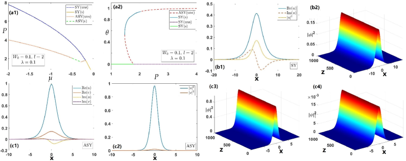
Figure 10: (a1) Total power $P$ versus propagation constant $-\mu$ for symmetric (SY) and asymmetric (ASY) GS modes in the case of the pure imaginary localized potential $W_{2}(x)$. (a2) Bifurcation diagrams in the $(P,\theta)$ plane for the imaginary potential $W_{2}(x)$ with $W_{0}=0.1$, $l=2$, and inter-core coupling constant $\lambda=0.1$. (b1,b2). The stable symmetric GS solution $u(x)=v(x)$ at $\mu=-0.18$ and its evolution. (c1-c4). Profiles $u(x)$ and $v(x)$ of the stable asymmetric GS solution at $\mu=-0.5$ and its evolution. Here “uns” and “s” represent, respectively, unstable and stable solutions, and the inter-core coupling constant is $\lambda=0.1$.

5 Management of symmetric and asymmetric GS modes via the variable $\mathcal{PT}$-symmetric potential or inter-core coupling

Finally, we aim to discuss dynamical transformation (“management”) of symmetric and asymmetric GS modes by making the potential parameter $W_{0}$ or coupling constant $\lambda$ functions of propagation distance $z$, i.e., we set $W_{0}=\widehat{W}_{0}(z)$ in Eqs. (3) and (4), and $\lambda=\widehat{\lambda}(z)$ in Eq. (2). The accordingly modified system is

$$\begin{split}i\phi_{z}&=-\frac{1}{2}\phi_{xx}-|\phi|^{2}\phi+(V(x)+i\widehat{W}(x,z))\phi-\widehat{\lambda}(z)\psi,\\ i\psi_{z}&=-\frac{1}{2}\psi_{xx}-|\psi|^{2}\psi+(V(x)+i\widehat{W}(x,z))\psi-\widehat{\lambda}(z)\phi.\end{split}$$ (19)

where $V(x)=\frac{1}{2}x^{2}$, and $\widehat{W}(x,z)$ is chosen as

$$\widehat{W}_{1}(x,z)=\widehat{W}_{0}(z)\tanh\left(\frac{x}{l}\right),$$ (20)

or

$$\widehat{W}_{2}(x,z)=\widehat{W}_{0}(z)\,\mathrm{sech}\left(\frac{x}{l}\right)\tanh\left(\frac{x}{l}\right),$$ (21)

Here we address two scenarios of the adiabatic variation of parameters $\widehat{W}_{0}(z)$ and $\widehat{\lambda}(z)$ in the form [cf. Ref. [63, 64, 65]]:

$$\chi(z)\!=\!\left\{\!\begin{array}[]{ll}\displaystyle\frac{\chi_{2}-\chi_{1}}{2}\left[1-\cos\left(\frac{10\pi z}{z_{\mathrm{max}}}\right)\right]+\chi_{1},&\displaystyle 0\leq z<\frac{z_{\mathrm{max}}}{10},\vspace{0.1in}\\ \chi_{2},&\displaystyle\frac{z_{\mathrm{max}}}{10}\leq z\leq z_{\mathrm{max}},\end{array}\right.$$ (22)

where $\chi_{1,2}$ stand for the initial and final values in the excitation, respectively, and $z_{\mathrm{max}}$ represents the maximal value of numerical simulations.

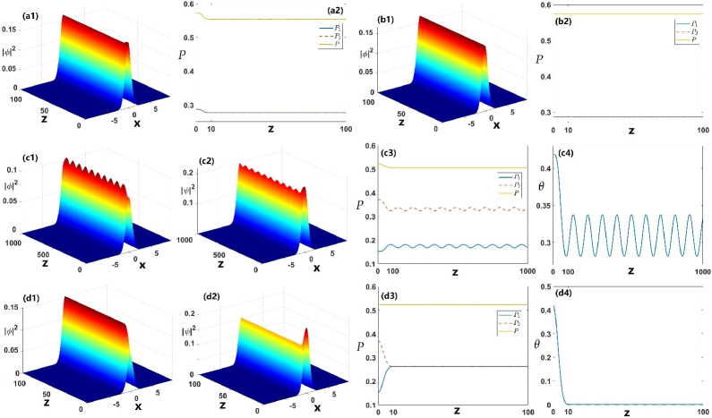
Figure 11: Transformation of GS modes in the framework of Eq. (22). The initial state corresponds to $W_{0}=0.5$, $l=2$ and $\mu=0.1$ ($P\approx 0.5734$). (a1,a2): The production of a symmetric GS mode by changing $W_{0}$ from ${\small 0.5}$ to $0.1$ and the corresponding power curve $P(z)$. (b1,b2): The production of a symmetric GS mode by changing $\lambda$ from 0.3 to $0.1$ and the corresponding power curve $P(z)$. The following panels display the production of asymmetric GS modes from the initial state corresponding to $W_{0}=0.5$, $l=2$ and $\mu=0.3$ ($P\approx 0.5232$). (c1,c2): The production of an asymmetric GS mode by changing $W_{0}$ from ${\small 0.5}$ to $0.1$. (c3,c4): The corresponding power curve $P(z)$ and asymmetry characteristic $\theta(z)$. (d1,d2): The production of an asymmetric GS mode by varying $\lambda$ from ${\small 0.2235}$ to $0$. (d3,d4): The corresponding power curve $P(z)$ and asymmetry characteristic $\theta(z)$.

We here consider the imaginary potential $\widehat{W}_{2}(x,z)$ given by Eq. (21). First, for symmetric GS modes, keeping $\widehat{\lambda}$ fixed and replacing $\widehat{W}_{0}(z)$ with $\chi(z)$ given by Eq. (22), we can adiabatically transform the initial state from $\chi_{1}=0.5$ to $\chi_{2}=0.1$, as shown in Fig. 11(a1). Figure 11(a2) displays the corresponding power curves $P(z)$. defined as per Eq. (6). It is seen that an initially stable symmetric GS mode with a higher power is transformed into another symmetric one with a lower power. Besides, for the same initial state, if we consider the varying coupling $\widehat{\lambda}(z)$, from $\chi_{1}=0.3$ to $\chi_{2}=0.1$, a stable symmetric GS mode is carried over into another symmetric one with the constant power, i.e., $\mathrm{d}P/\mathrm{d}z=0$ (see Eq. (7) and Figs. 11(b1,b2)). Therefore, the symmetric sates can only be converted into another symmetric one, in the framework of system (19).

Next, a question is if an asymmetric state can be converted into a symmetric one. First, for fixed $\widehat{\lambda}$, an initially stable asymmetric state is transformed into an asymmetric one with residual oscillations, if $\widehat{W}_{0}(z)$ is taken as per Eq. (22) with $\chi_{1}=0.5$ to $\chi_{2}=0.1$ (see Figs. 11(c1,c2)). The corresponding power curve $P(z)$ and asymmetry characteristic $\theta(z)$ are displayed in Fig. 11(c3,c4). Powers $P_{1}$ and $P_{2}$ feature oscillations, while the total power $P$ remains constant. If we only consider the varying inter-core coupling $\widehat{\lambda}(z)$ with $\chi_{1}=0.2235$ to $\chi_{2}=0$, the stable asymmetric state is transformed into a stable symmetric one, as shown in Figs. 11(d1-d4). A condition necessary for the implementation of this conversion is $P_{1}(z_{\mathrm{max}}/10)=P_{2}(z_{\mathrm{max}}/10)$. It is observed in Fig. 11(d4) that, at $z\geq z_{\mathrm{max}}/10=10$, a stable symmetric state appears with $\theta=0$.

Similar results can be obtained for the imaginary potential $\widehat{W}_{1}(x,z)$ given by Eq. (20), which are not presented here in detail.

6 Physical interpretations

In Fig. 1, we show the profiles of real and imaginary parts of the ${\cal PT}$-symmetryic potentials and the ${\cal PT}$ symmetry breaking of the linear spectral problem (13) with differential gain-and-loss distributions given by Eqs. (3) and (4). In Fig. 2, we exhibit the boundary for the breaking of the inter-core symmetry $P_{\mathrm{cr}}(\lambda)$ and $\mu_{\mathrm{cr}}$. Total power $P$ versus propagation constant for GS modes is shown in Fig. 3. The important results are displayed in Fig. 4, i.e., the stability and boundary of the breaking of the inter-core symmetry for GS modes in $(W_{0},P)$-space. It is found that the instability of ${\cal PT}$-symmetric solutions takes place prior to the inter-core symmetry breaking. And, stable inter-core-symmetric GS solutions may remain stable while the ${\cal PT}$ symmetry is broken. Fig. 5 shows the asymmetry characteristic $\theta$ (see Eq. (12)) in $(W_{0},P)$-space. And Fig. 7 exhibits the stability and boundary of the breaking of the inter-core symmetry for DM modes in $(W_{0},P)$-space. Besides, Figs. 6, 8 and 9 show the profiles of GS and DM modes as well as the corresponding numerically simulated evolution. Fig. 10 displays the total power versus propagation constant for GS modes in the case of the pure imaginary localized potential $W_{2}(x)$. Finally, the transformation of GS modes in the framework of Eq. (22) is shown in Fig. 11.

7 Conclusions and discussions

In this work, we have introduced the one-dimensional system of linearly coupled NLS equations with the cubic self-attraction, harmonic-oscillator trapping potential, and two different types of the spatially odd dissipative potential (gain-loss distribution), localized and delocalized. The system models the light transmission in a dual-core planar waveguide (coupler) with the Kerr nonlinearity and effective $\mathcal{PT}$-symmetric potential. By means of numerical methods, symmetric and asymmetric GS (ground-state) and DM (dipole-mode) solitons have been found. Due to the action of the harmonic-oscillator trap, it is possible to find stable dipole modes in dissipative systems. The asymmetric states are generated from symmetric ones by the SBB (ground-state) of the supercritical type. The novelty of results in the system is interplay between breakings of the ${\cal PT}$ and inter-core symmetries. In order to exhibit the feature, the critical value of the power, $P_{\mathrm{cr}}$, at which the breaking of the inter-core symmetry takes place, is found as a function of strength $W_{0}$ of the gain-loss distribution. The stability of symmetric and asymmetric GS and DM modes, affected by the SBB and $\mathcal{PT}$-symmetry breaking, is investigated by dint of the linear-stability analysis and direct simulations. Different from the conservative counterpart of the system, with $W_{0}=0$, the instability of the symmetric GS solutions commences prior to the onset of the inter-core symmetry breaking, due to the effect of the gain-loss distribution. Near the $\mathcal{PT}$-symmetry breaking point, instability of the symmetric solution sets in at smaller values of the power. Surprisingly, stable inter-core-symmetric GS solutions may remain stable while the ${\cal PT}$ symmetry is broken. In contrast to the conservative system, in which all asymmetric states created by the supercritical SBB are stable, in the present system, which includes the imaginary potential, asymmetric GS and DM are only partly stable. We have also investigated the SBB of symmetric and asymmetric GS modes in the system including a localized pure imaginary potential, in the absence of the real potential. In this case, the SBB is of the subcritical type. And stable solitons can still be found in dissipative systems. Finally, the transformation of symmetric and asymmetric GS modes has been studied, following variation of the strength of the imaginary potential $W_{0}$ or inter-core coupling constant $\lambda$ along the propagation distance, which demonstrate that the GS modes can be transformed from the asymmetric shape into the symmetric one, under appropriate conditions. These results may provide the theoretical support for the optical experiments in a dual-core planar waveguide with ${\cal PT}$-symmetric potential.

This work suggests an interesting extension for the study of SBB of fundamental and vortical two-component solutions in the effectively two-dimensional spatiotemporal dual-core system [66] with a $\mathcal{PT}$-symmetric potential.

$$\begin{split}i\phi_{z}&=-\frac{1}{2}\nabla^{2}\phi+F(|\phi|^{2},|\psi|^{2})\phi+[V({\bf r})+iW({\bf r})]\phi-\kappa\psi,\\ i\psi_{z}&=-\frac{1}{2}\nabla^{2}\psi+F(|\phi|^{2},|\psi|^{2})\psi+[V({\bf r})+iW({\bf r})]\psi-\kappa\phi.\end{split}$$ (23)

It may also be relevant to consider a generalization of the system including an optical-lattice potential, which may give rise to other asymmetric soliton modes.

Authors’ contributions. J.S.: Conceptualization, Methodology, Investigation, Analysis, Writing-original draft. B.A.M. and Z.Y.: Conceptualization, Methodology, Formal Analysis, Supervision, Funding acquisition, Writing-reviewing and editing.

Conflict of interest declaration. We declare we have no competing interests.

Funding. Z.Y. acknowledges support from the National Nature Science Foundation of China under Grant No. 11925108. The work of B.A.M. is supported, in part, by the Israel Science Foundation through grant No. 1695/22.

References

- [1] Landau D., and Lifshitz, E. M. Quantum Mechanics (Nauka Publishers, Moscow, 1974).
- [2] Agrawal, G. P. Nonlinear Fiber Optics (Academic Press, Amsterdam, 2013).
- [3] Malomed, B. A. (ed) Spontaneous Symmetry Breaking, Self-Trapping, and Josephson Oscillations (Springer, Berlin, 2013).
- [4] Jensen, S. M. The nonlinear coherent coupler, IEEE J. Quant. Elect., 1982, QE-18, 1580-1583.
- [5] Chen, Z., Li, Y., Malomed, B. A., and Salasnich, L. Spontaneous symmetry breaking of fundamental states, vortices, and dipoles in two and one-dimensional linearly coupled traps with cubic self-attraction, Phys. Rev. A, 2017, 96, 033621.
- [6] Wright, E. M., Stegeman, G. I., and Wabnitz, S. Solitary-wave decay and symmetry-breaking instabilities in two-mode fibers, Phys. Rev. A, 1989, 40, 4455-4466.
- [7] Paré, C., and Fłorjańczyk, M. Approximate model of soliton dynamics in all-optical couplers, Phys. Rev. A, 1990, 41, 6287-6295.
- [8] Maimistov, A. I. Propagation of a light pulse in nonlinear tunnel-coupled optical waveguides, Kvant. Elektron., 18, 758-761 [Sov. J. Quantum Electron.,1991, 21, 687-690].
- [9] Snyder, A. W., Mitchell, D. J., Poladian, L., Rowland, D. R., and Chen, Y. Physics of nonlinear fiber couplers, J. Opt. Soc. Am. B, 1991, 8, 2101-2118.
- [10] Akhmediev, N., and Ankiewicz, A. Novel soliton states and bifurcation phenomena in nonlinear fiber couplers, Phys. Rev. Lett., 1993, 70, 2395-2398.
- [11] Malomed, B. A., Skinner, I., Chu, P. L., and Peng, G. D. Symmetric and asymmetric solitons in twin-core nonlinear optical fibers, Phys. Rev. E, 1996, 53, 4084.
- [12] Nguyen, V. H., Tai, L. X. T., Bugar, I., Longobucco, M., Buzcynski, R., Malomed, B. A., and Trippenbach, M. Reversible ultrafast soliton switching in dual-core highly nonlinear optical fibers, Opt. Lett., 2020, 45, 5221-5224.
- [13] Iooss, G. and Joseph, D. D. Elementary Stability Bifurcation Theory (Springer-Verlag: New York, 1980).
- [14] Dikwa, J., Houwe, A., Abbagari, S., Akinyemi, L., and Inc, M. Modulated waves patterns in the photovoltaic photorefractive crystal, Opt. Quant. Electron, 2022, 54(12), 842.
- [15] Abbagari, S., Houwe, A., Doka, S. Y., Inc, M., and Bouetou, T. B. Specific optical solitons solutions to the coupled Radhakrishnan–Kundu–Lakshmanan model and modulation instability gain spectra in birefringent fibers, Opt. Quant. Electron, 2022, 54, 1-25.
- [16] Abbagari, S., Houwe, A., Akinyemi, L., Inc, M., Doka, S. Y., and Crepin, K. T. Synchronized wave and modulation instability gain induce by the effects of higher-order dispersions in nonlinear optical fibers, Opt. Quant. Electron, 2022, 54(10), 642.
- [17] Inan, I. E., Inc, M., Rezazadeh, H., and Akinyemi, L. Optical solitons of (3+1) dimensional and coupled nonlinear Schrodinger equations, Opt. Quant. Electron, 2022, 54(4), 261.
- [18] Sigler, A., and Malomed, B. A. Solitary pulses in linearly coupled cubic-quintic Ginzburg-Landau equations, Physica D, 2005, 212, 305-316.
- [19] Heil, T., Fischer, I., Elsässer, W., Mulet, J., and Mirasso, C. R. Chaos synchronization and spontaneous symmetry-breaking in symmetrically delay-coupled semiconductor lasers. Phys. Rev. Lett., 2000, 86, 795-798.
- [20] Bender, C. M., and Boettcher, S. Real spectra in non-hermitian hamiltonians having symmetry, Phys. Rev. Lett., 1998, 80, 5243.
- [21] Bagchi, B., and Roychoudhury, R. A new -symmetric complex hamiltonian with a real spectrum, J. Phys. A, 2000, 33, L1.
- [22] Ahmed, Z. Real and complex discrete eigenvalues in an exactly solvable one-dimensional complex -invariant potential, Phys. Lett. A, 2001, 282, 343.
- [23] Musslimani, Z., Makris, K. G., El-Ganainy, R., and Christodoulides, D. N. Beam dynamics in Symmetric Optical Lattices, Phys. Rev. Lett., 2008, 100, 030402.
- [24] Bender, C. M. Making sense of non-Hermitian Hamiltonians, Rep. Prog. Phys., 2007, 70, 947.
- [25] Makris, K. G., El-Ganainy, R., Christodoulides, D. N. and Musslimani, Z. H. -Symmetric periodic optical potentials, Int. J. Theor. Phys., 2011, 50, 1019-1041.
- [26] Suchkov, S. V., Sukhorukov, A. A., Huang, J., Dmitriev, S. V., Lee, C., and Kivshar, Y. S. Nonlinear switching and solitons in -symmetric photonic systems, Laser Photonics Rev., 2016, 10, 177-213.
- [27] Konotop, V. V., Yang, J., and Zezyulin, D. A. Nonlinear waves in -symmetric systems, Rev. Mod. Phys., 2016, 88, 035002.
- [28] Longhi, S. Bloch oscillations in complex crystals with symmetry, Phys. Rev. Lett. 2009, 103, 123601.
- [29] Sun, C., Barsi, C., and Fleischer, J. W. Peakon profiles and collapse-bounce cycles in self-focusing spatial beams, Opt. Exp., 2008, 16, 20676-20686.
- [30] Conti, C., Fratalocchi, A., Peccianti, M., Ruocco, G., and Trillo, S. Observation of a gradient catastrophe generating solitons, Phys. Rev. Lett., 2009, 102, 083902.
- [31] Abdullaev, F.K. , Kartashov, Y. V., Konotop, V. V., and Zezyulin, D. A. Solitons in PT-symmetric nonlinear lattices, Phys. Rev. A 2009, 83, 041805(R).
- [32] Bludov, Y. V., Konotop, V. V., and Malomed, B. A. Stable dark solitons in PT-symmetric dual-core waveguides, Phys. Rev. A 2013, 87, 013816.
- [33] Zeng, J., and Lan, Y. Two-dimensional solitons in PT linear lattice potentials, Phys. Rev. E 2012, 85, 047601.
- [34] Zhong, W. P., Belić, M., & Huang, T. Two-dimensional accessible solitons in PT-symmetric potentials. Nonlinear Dyn. 2012, 70, 2027-2034.
- [35] Dai, C., Wang, X., and Zhou, G. Stable light-bullet solutions in the harmonic and parity-time-symmetric potentials, Phys. Rev. A 2014, 89, 013834.
- [36] Kevrekidis, P.G., Cuevas-Maraver, J., Saxena, A., and Cooper, F. Interplay between parity-time symmetry, supersymmetry, and nonlinearity: An analytically tractable case example, Phys. Rev. E 2015, 92, 042901.
- [37] Yan, Z., Wen, Z., Hang, C. Spatial solitons and stability in self-focusing and defocusing Kerr nonlinear media with generalized parity-time-symmetric Scarf-II potentials, Phys. Rev. E 2015, 92, 022913.
- [38] Li, P., and Mihalache, D. Symmetry breaking of solitons in PT-symmetric potentials with competing cubic-quintic nonlinearity, Proc. Rom. Acad. A 2018, 19, 61.
- [39] Zhong, M., Chen, Y., Yan, Z., and Tian, S.-F. Formation, stability, and adiabatic excitation of peakons and double-hump solitons in parity-time-symmetric Dirac--Scarf-II optical potentials, Phys. Rev. E 2022, 105, 014204.
- [40] Yang, J. Symmetry breaking with opposite stability between bifurcated asymmetric solitons in parity-time-symmetric potentials. Opt. Lett. 2019, 44(11), 2641.
- [41] Li, P., Dai, C., Li, R., and Gao, Y. Symmetric and asymmetric solitons supported by a PT-symmetric potential with saturable nonlinearity: bifurcation, stability and dynamics. Opt. Exp. 2018, 26(6), 6949-6961.
- [42] Dong, L., Huang, C., and Qi, W. Symmetry breaking and restoration of symmetric solitons in partially parity-time-symmetric potentials. Nonlinear Dyn. 2019, 98(3), 1701-1708.
- [43] Bo, W., Dai, C., Wang, Y., and Li, P. Symmetry breaking of PT-symmetric solitons in self-defocusing saturable nonlinear Schrödinger equation, 2021, DOI:10.21203/rs.3.rs-725749/v1.
- [44] Rüter, C. E., Makris, K. G., El-Ganainy, R., Christodoulides, D. N., Segev, M., and Kip, D. Observation of parity-time symmetry in optics, Nature Physics, 2010, 6, 192-195.
- [45] Guo, A., Salamo, G., Duchesne, D., Morandotti, R., Volatier-Ravat, M., Aimez, V., Siviloglou, G., and Christodoulides, D. N. Observation of -symmetry breaking in complex optical potentials, Phys. Rev. Lett., 2009, 103(9), 093902.
- [46] Driben, R., and Malomed, B. A. Stability of solitons in parity-time-symmetric couplers, Opt. Lett., 2011, 36, 4323-4325.
- [47] Alexeeva, N. V., Barashenkov, I. V., Sukhorukov, A. A., and Kivshar, Y. S. Optical solitons in -symmetric nonlinear couplers with gain and loss, Phys. Rev. A, 2012, 85, 063837.
- [48] Siegman, A. E., Lasers (University Science Books, Sausalito, CA, 1986).
- [49] Mayteevarunyoo, T., Malomed, B. A., and Skryabin, D. V. One- and two-dimensional modes in the complex Ginzburg-Landau equation with a trapping potential, Opt. Exp., 2018, 26, 8849-8865.
- [50] Moiseyev, N. Non-Hermitian Quantum Mechanics (Cambridge University Press, Cambridge, 2011).
- [51] Malomed, B. A. Variational methods in nonlinear fiber optics and related fields, Progr. Optics 2002, 43, 71-193.
- [52] Yang, J. Nonlinear Waves in Integrable and Nonintegrable Systems (SIAM, 2010).
- [53] Yang, J., and Lakoba, T. I. Universally-convergent squared-operator iteration methods for solitary waves in general nonlinear wave equations, Stud. Appl. Math., 2007, 118, 153-197.
- [54] Mertens, F., Cooper, F., Arevalo, E., Khare, A., Saxena, A., and Bishop, A., Variational approach to studying solitary waves in the nonlinear Schrödinger equation with complex potentials. Phys. Rev. E 2016, 94, 032213.
- [55] Charalampidis, E., Dawson, J., Cooper, F., Khare, A., and Saxena, A., Stability and response of trapped solitary wave solutions of coupled nonlinear Schrödinger equations in an external, - and supersymmetric potential. J. Phys. A: Math. Theor. 2020, 53, 455702.
- [56] Charalampidis, E., Cooper, F., Dawson, J., K. Avinash, and Saxena, A., Behavior of solitary waves of coupled nonlinear Schrödinger equations subjected to complex external periodic potentials with odd- symmetry, J. Phys. A: Math. Theor. 2021, 54 145701.
- [57] Trefethen, L. N. Spectral Methods in Matlab (SIAM, 2000).
- [58] Pitaevskii, L. P. and Stringari, S. Bose-Einstein Condensation (Oxford University Press, Oxford, 2003).
- [59] Vakhitov, N. G., Kolokolov, A. A. Stationary solutions of the wave equation in a medium with nonlinearity saturation, Izv. Vyssh. Uchebn. Zaved. Radiofzi., 1973, 16, 1020.
- [60] Bergé, L. Wave collapse in physics: principles and applications to light and plasma waves, Phys. Rep., 1998, 303, 259-370.
- [61] Sulem, C., and Sulem, P.-L. The Nonlinear Schrödinger Equation: Self-Focusing and Wave Collapse (Springer, New York, 1999).
- [62] Fibich, G. The Nonlinear Schrödinger Equation: Singular Solutions and Optical Collapse (Springer, Heidelberg, 2015).
- [63] Yan, Z., Wen, Z., and Konotop, V. V. Solitons in a nonlinear Schrödinger equation with -symmetric potentials and inhomogeneous nonlinearity: Stability and excitation of nonlinear modes, Phys. Rev. A, 2015, 92, 023821.
- [64] Song, J., Zhou, Z., Dong, H., and Yan, Z. Stable solitons and peakons, quantum information entropies, interactions, and excitations for generalized PT-symmetric NLS equations, Wave Motion 2022, 115, 103076.
- [65] Song, J., Zhou, Z., Weng, W., and Yan, Z. PT-symmetric peakon solutions in self-focusing/defocusing power-law nonlinear media: Stability, interactions and adiabatic excitations, Physica D 2022, 435, 133266.
- [66] Dror, N., and Malomed, B. A. Symmetric and asymmetric solitons and vortices in linearly coupled two-dimensional waveguides with the cubic-quintic nonlinearity, Physica D, 2011, 240, 526-541.