Data-driven re-evaluation of $ft$-values in superallowed beta decays

Abstract

We present a comprehensive re-evaluation of the $ft$-values in superallowed nuclear beta decays crucial for the precise determination of $V_{ud}$ and low-energy tests of the electroweak Standard Model. It consists of the first, fully data-driven analysis of the nuclear beta decay form factor, that utilizes isospin relations to connect the nuclear charged weak distribution to the measurable charge distributions. This prescription supersedes previous shell-model estimations, and allows for a rigorous quantification of theory uncertainties in $f$ which is absent in the existing literature. Our new evaluation shows an overall downward shift of the central values of $f$ at the level of 0.01%.

I Introduction

The top-row Cabibbo-Kobayashi-Maskawa (CKM) matrix element $V_{ud}$ is a fundamental parameter in the Standard Model (SM) that governs the strength of charged weak interactions involving up and down quarks. Its precise determination constitutes an important component of the low-energy tests of SM and the search of physics beyond the Standard Model (BSM) at the precision frontier. Currently, beta transitions between isospin $T=1$, and spin-parity $J^{P}=0^{+}$ nuclear states (the so-called superallowed nuclear beta decays) and free neutron are the two competing candidates for the most precise determination of $V_{ud}$. The advantage of the former is the existence of the many nuclear transitions that had been measured over decades and averaged over (see, e.g. Reg.Hardy and Towner (2020) and references therein), but the existence of nuclear structure effects complicates the theory analysis. In contrast, neutron decay is limited by the experimental precision but is free from nuclear uncertainties and is theoretically cleaner.

The recent improved measurement of the neutron lifetime $\tau_{n}$ by UCN$\tau$ Gonzalez et al. (2021) and the axial coupling constant $g_{A}$ by PERKEO-III Märkisch et al. (2019) have made the precision of $V_{ud}$ from neutron beta decay almost comparable to that from superallowed nuclear beta decays, but a mild tension starts to develop between the two values:

$$|V_{ud}|_{0^{+}}=0.97361(31)\leavevmode\nobreak\ \text{\cite[cite]{\@@bibref{Authors Phrase1YearPhrase2}{Hardy:2020qwl}{\@@citephrase{(}}{\@@citephrase{)}}}}\leavevmode\nobreak\ ,\quad|V_{ud}|_{n}^{\text{best}}=0.97404(42)\leavevmode\nobreak\ \text{\cite[cite]{\@@bibref{Authors Phrase1YearPhrase2}{Gorchtein:2023srs}{\@@citephrase{(}}{\@@citephrase{)}}}}\leavevmode\nobreak\ .$$ (1)

Combining them with the best determination of $V_{us}$ from semileptonic kaon decays, $|V_{us}|_{K_{\ell 3}}=0.22308(55)$ Seng et al. (2022a, b) (with $N_{f}=2+1+1$ lattice determination of the $K^{0}\rightarrow\pi^{-}$ transition matrix element Carrasco et al. (2016); Bazavov et al. (2019); Aoki et al. (2022)), and $|V_{ub}|_{K_{\ell 3}}=3.82(20)\times 10^{-3}$ Workman et al. (2022), the first number leads to a $3.6\sigma$ deficit of the first-row CKM unitarity $|V_{ud}|^{2}+|V_{us}|^{2}+|V_{ub}|^{2}=1$, but with the second number the deficit is only $1.7\sigma$. Given its profound impact on the SM precision tests, it is important to understand the origin of such discrepancy. It is a commonplace for low-energy precision tests that the main limitation in precision comes from radiative corrections that are sensitive to the effects of strong interaction which is described by Quantum Chromodynamics (QCD). At low energies QCD is nonperturbative, which complicates the uncertainty estimation of theory calculations. In the recent years, effort has been put in developing methods that would allow to compute such corrections to beta decay with a controlled systematics. The dispersion relation (DR) Seng et al. (2018, 2019); Shiells et al. (2021), effective field theory (EFT) Cirigliano et al. (2022, 2023) and lattice QCD Feng et al. (2020); Yoo et al. (2023); Ma et al. (2023) analyses have ensured a high-precision determination of the single-nucleon radiative correction. The SM theory uncertainties in the free neutron decay are believed to be firmly under control at the precision level of $10^{-4}$.

The theory for superallowed nuclear beta decays is more involved due to the presence of specifically nuclear corrections. This fact is reflected in the master formula for the extraction of $V_{ud}$ Hardy and Towner (1975),

$$|V_{ud}|_{0^{+}}^{2}=\frac{\pi^{3}\ln 2}{G_{F}^{2}m_{e}^{5}\mathcal{F}t(1+\Delta_{R}^{V})}\leavevmode\nobreak\ .$$ (2)

Above, $\Delta_{R}^{V}$ is the free-nucleon radiative correction which is also present in neutron decay. All nuclear structure effects are absorbed into the so-called $\mathcal{F}t$-value Towner and Hardy (2002),

$$\mathcal{F}t=ft(1+\delta_{\text{R}}^{\prime})(1+\delta_{\text{NS}}-\delta_{\text{C}})\leavevmode\nobreak\ ,$$ (3)

where $t$, the partial half-life, is the only pure experimental observable. All the remaining quantities in the expression above require nuclear theory inputs at either tree or loop level. First, $\delta_{\text{R}}^{\prime}$ is known as the nucleus-dependent outer radiative correction, which is calculable order-by-order with Quantum Electrodynamics (QED) assuming the nucleus as a point charge Sirlin (1967, 1987); Sirlin and Zucchini (1986). The remaining radiative corrections that depend on the nuclear structure are contained in $\delta_{\text{NS}}$, which has previously been studied in the nuclear shell model Barker et al. (1992); Towner (1992, 1994); Towner and Hardy (2002, 2008). Furthermore, $\delta_{\text{C}}$ represents the isospin-symmetry-breaking (ISB) correction to the Fermi matrix element. This correction has been object of study by the nuclear theory community over the past 6 decades MacDonald (1958); Towner and Hardy (2008); Satuła et al. (2016); Ormand and Brown (1995); Liang et al. (2009); Auerbach (2009). Both $\delta_{\text{NS}}$ and $\delta_{\text{C}}$ have recently been under renewed scrutiny Miller and Schwenk (2008, 2009); Seng et al. (2019); Gorchtein (2019); Condren and Miller (2022), and new methods were devised to study them either using nuclear ab-initio methods Seng and Gorchtein (2023a, b) or by relating them to experimental measurements Seng and Gorchtein (2023c), which we will not discuss here.

The focus of this paper is the statistical rate function $f$ in superallowed beta decays. It represents the phase space integral over the spectrum of the positron originating from a beta decay process $\phi_{i}\rightarrow\phi_{f}e^{+}\nu_{e}$. At the leading order it is fixed by the atomic mass splitting (i.e. the $Q_{\text{EC}}$ value). However, a number of effects that lead to sizable corrections to the spectrum have to be included $f$, that require theory inputs from atomic and nuclear physics. Among these count the distortion of the outgoing positron wave function in the Coulomb field of the daughter nucleus, the nuclear form factors, screening effects from atomic electrons, recoil corrections etc. In principle, each of these inputs bears its own theory uncertainty which must be accounted for in the total error budget. Unfortunately, in most existing literature, including the series of reviews by Hardy and Towner Hardy and Towner (2005, 2009, 2015, 2020), only the experimental uncertainty of $Q_{\text{EC}}$ is included in the evaluation of $f$. Here we address the validity of this assumption, given the precision goal of $10^{-4}$ for the extraction of $V_{ud}$.

A quantity of fundamental importance in the determination of the statistical rate function is the charged weak form factor $f_{+}(q^{2})$, defined through the (relativistic) nuclear matrix element of the vector charged current:

$${}_{\text{QFT}}\langle\phi_{f}(p_{f})|(J_{W}^{\dagger\mu}(0))_{V}|\phi_{i}(p_{i})\rangle_{\text{QFT}}$$

$$=f_{+}(q^{2})(p_{i}+p_{f})^{\mu}+f_{-}(q^{2})(p_{i}-p_{f})^{\mu}\leavevmode\nobreak\ ,$$ (4)

with $q^{2}=(p_{i}-p_{f})^{2}$. In nuclear physics it is common to use the Breit frame where $q$ only has the spatial component. The contribution of $f_{-}$ to the decay rate is suppressed simultaneously by ISB and kinematics, so only $f_{+}$ is relevant. After scaling out its $\vec{q\,}^{2}=0$ value which is just the Fermi matrix element $M_{F}$ ($=\sqrt{2}$ in the isospin limit), one can perform a Fourier transform

$$f_{+}(q^{2})=M_{F}\int d^{3}xe^{-i\vec{q}\cdot\vec{x}}\rho_{\text{cw}}(r)\leavevmode\nobreak\ ,$$ (5)

which defines the nuclear charged weak distribution $\rho_{\text{cw}}(r)$; it is essentially the distribution of “active” protons eligible to transition weakly into a neutron in a nucleus. Obviously, $\rho_{\text{cw}}(r)$ is a basic property of the nucleus, just like the nuclear charge distribution $\rho_{\text{ch}}(r)$. Yet, in the literature they are treated with very different levels of rigor: $\rho_{\text{ch}}(r)$ was deduced from experimental data where uncertainties are (in principle) quantifiable, whereas $\rho_{\text{cw}}(r)$ is evaluated using simplified nuclear models. This may introduce an uncontrolled systematic uncertainty and neglects the fact that the two distributions are correlated.

The purpose of this paper is to perform a careful re-evaluation of $f$ with a more rigorous, data-driven error analysis. In particular, we adopt the strategy pioneered in Ref.Seng (2023) that connects $\rho_{\text{cw}}(r)$ to the charge distributions of the members of the superallowed isotriplet using model-independent isopsin relations. This prescription transforms the non-quantifiable model uncertainty in the usual approach to $\rho_{\text{cw}}(r)$ into uncertainty estimates that are derived from experimental ones under the only assumption of an approximate isospin symmetry. Furthermore, the new approach automatically accounts for the correlation between the Fermi function and decay form factor, and treats their uncertainties on the same footing. We furthermore analyse possible uncertainties from secondary effects, such as the screening corrections by the atomic electrons. With these, we report a set of 13 newly-calculated $f$, with a much more robust uncertainty estimate. Our result lays a foundation for the future, more rigorous extraction of $V_{ud}$ from superallowed beta decays.

This work is organized as follows. In Sec.II we introduce the statistical rate function specifying various correction terms. A particular emphasis is put on the shape factor that depends on the charged weak distribution. In Sec.III we describe the isospin relations that connect different electroweak distribution functions. Sec.D is the central part of this work, where we describe in full detail our procedure of selecting the nuclear charge distribution data that we use for the data-driven analysis. In Sec.V we discuss our treatment of the secondary nuclear/atomic structure effects that enter $f$. We present our final results in Sec.VI and discuss their influence and prospects. Some useful formulas on the solutions of the Dirac equation, the shape factor and the nuclear charge distributions can be found in the Appendix.

II Statistical rate function and the shape factor

We study the superallowed $\beta^{+}$ decay, $\phi_{i}\rightarrow\phi_{f}e^{+}\nu_{e}$, where we denote the positron energy and momentum as as $E\equiv E_{e}$ and $\vec{p}\equiv\vec{p}_{e}$, with $\mathbf{p}=|\vec{p}|$. The positron end-point energy of the decay is given by $E_{0}^{\text{full}}\equiv(M_{i}^{2}-M_{f}^{2}+m_{e}^{2})/(2M_{i})$, but upon neglecting recoil corrections it can be approximated as $E_{0}\equiv M_{i}-M_{f}$. Before applying various corrections, the uncorrected differential decay rate is proportional to $\mathbf{p}E(E_{0}-E)^{2}$. The statistical rate function $f$ is defined as the integrated decay rate in atomic units ($\hbar=c=m_{e}=1$).

Ref.Hayen et al. (2018) provided an in-depth survey of some 12 different types of atomic/nuclear corrections that should be applied to formula above for a generic allowed beta decay. For superallowed decays of $0^{+}$ nuclei, the number of relevant corrections is reduced. Therefore, following Refs.Hardy and Towner (2005, 2009), we express the statistical rate function as

$$f=m_{e}^{-5}\int\limits_{m_{e}}^{E_{0}}\mathbf{p}E(E_{0}-E)^{2}F(E)C(E)Q(E)R(E)r(E)dE\,,$$ (6)

where we have arranged the corrections factor in decreasing degrees of importance: (1) The Fermi function $F(E)$, (2) The shape factor $C(E)$, (3) The atomic shadowing correction $Q(E)$, (4) The kinematic recoil correction $R(E)$, and (5) The atomic overlap correction $r(E)$. All the five corrections depend on the nucleus, which is usually denoted by carrying the daughter nucleus charge $Z$ as a second argument, but we suppress this dependence for compactness. In this work we classify the former two corrections as primary, which will be evaluated coherently using the most recent nuclear distribution data. The latter three corrections, on the other hand, are classified as secondary and we will not treat them differently than in the literature (except for a more careful account for theory uncertainties).

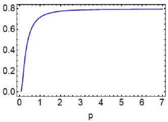
Figure 1: A plot of the Fermi function $F(E)$ with respect to $\mathbf{p}$ (in units of $m_{e}$) for ²²Mg. The error band due to uncertainties from the nuclear charged distribution parameters is too small to be visible.

We start from the largest correction, the Fermi function $F(E)$ that accounts for the Coulomb interaction between the outgoing positron and the daughter nucleus Fermi (1934). Historically, it was first derived by solving the Dirac equation of the charged lepton under the Coulomb potential of a point-like nucleus, which the equation is analytically solvable. The solution diverges at $r=0$, so it was instead evaluated at an arbitrarily-chosen nuclear radius $R$ Konopinski and Uhlenbeck (1941); corrections due to the finite nuclear charge distributions could then be added on top of it Behrens and Jänecke (1969); Calaprice and Holstein (1976). Here we do not adopt this two-step approach, but rather solving the full Dirac equation numerically with a given nuclear charge distribution. The numerical solution is finite at $r=0$, from which we can define the Fermi function as:

$$F(E)=\frac{f_{+1}^{2}(0)+g_{-1}^{2}(0)}{2\mathbf{p}^{2}}=\frac{\alpha_{+1}^{2}+\alpha_{-1}^{2}}{2\mathbf{p}^{2}}\leavevmode\nobreak\ ,$$ (7)

where the coefficients $\alpha_{\pm k}$ ($k=1$ in this case) come from the solution of the radial Dirac equation, detailed in Appendix A and B. Fig.1 shows the typical shape of the Fermi function for $\beta^{+}$ decay: since the Coulomb force is repulsive for a positron, the probability of its existence at $r=0$ with low energy is suppressed.

The second largest correction is the shape factor $C(E)$, which incorporates the influence of the beta decay form factor in Eq.(4) (or equivalently, the charged weak distribution in Eq.(5)). A closed expression was obtained by Behrens and Bühring Behrens and Bühring (1982):

$$C(E)=\sum_{k}\lambda_{k}\left\{M_{0}^{2}(k)+m_{0}^{2}(k)-\frac{2\mu_{k}\gamma_{k}}{kE}M_{0}(k)m_{0}(k)\right\}\leavevmode\nobreak\ ,$$ (8)

where $k=+1,+2,...$. The involved Coulomb functions are

$$\lambda_{k}=\frac{\alpha_{-k}^{2}+\alpha_{+k}^{2}}{\alpha_{-1}^{2}+\alpha_{+1}^{2}}\leavevmode\nobreak\ ,\leavevmode\nobreak\ \mu_{k}=\frac{\alpha_{-k}^{2}-\alpha_{+k}^{2}}{\alpha_{-k}^{2}+\alpha_{+k}^{2}}\frac{kE}{\gamma_{k}}\leavevmode\nobreak\ ,$$ (9)

where $\gamma_{k}=\sqrt{k^{2}-\alpha^{2}Z_{f}^{2}}$, with $Z_{f}$ the atomic number of the daughter nucleus. The functions that depend on $\rho_{\text{cw}}(r)$ are:

$$M_{0}(k) = \frac{\sqrt{k}}{(2k-1)!!}\int_{0}^{\infty}4\pi r^{2}dr\rho_{\text{cw}}(r)(\mathbf{p}r)^{k-1}$$

$$\times\left[H_{k}(r)j_{k-1}(E_{\nu}r)-\frac{r}{R}D_{k}(r)j_{k}(E_{\nu}r)\right]$$

$$m_{0}(k) = \frac{\sqrt{k}}{(2k-1)!!}\int_{0}^{\infty}4\pi r^{2}dr\rho_{\text{cw}}(r)(\mathbf{p}r)^{k-1}$$ (10)

$$\times\left[h_{k}(r)j_{k-1}(E_{\nu}r)-\frac{r}{R}d_{k}(r)j_{k}(E_{\nu}r)\right]\leavevmode\nobreak\$$

where $E_{\nu}\approx E_{0}-E$ is the neutrino energy, and the functions $H_{k}$, $h_{k}$, $D_{k}$ and $d_{k}$ are defined in Eq.(37). Notice that the overall Fermi matrix element has been factored out from the definitions above. The derivation of this master formula can be found in Appendix C. One can also check that it reduces to the simple expression in Ref.Seng (2023) upon switching off the electromagnetic interaction.

The series in Eq.8 converges very fast. In fact, explicit calculation shows that the $k=2$ correction to $f$ is smaller than 0.0003% for all measured transitions (i.e. up to $A=74$), therefore it is sufficient retain only the $k=1$ term which greatly simplifies the analysis.

III Isospin formalism

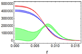
Figure 2: Plot of the nuclear charge distribution $\rho_{\text{ch}}(r)$ in atomic units ($\hbar=c=m_{e}=1$) for ²²Mg (blue), ²²Ne (red), and the corresponding charged weak distribution $\rho_{\text{cw}}(r)$ (green). The selection of nuclear charge distribution data is explained in Sec.IV.

In the survey by Hardy and Towner Hardy and Towner (2005), the weak form factor was evaluated in the impulse approximation where nucleus is treated as a collection of non-interacting nucleons. In this formalism, the nuclear matrix element of the weak transition operator $\hat{O}$ reads

$$\langle\phi_{f}|\hat{O}|\phi_{i}\rangle=\sum_{\alpha\beta}\langle\alpha|\hat{O}|\beta\rangle\langle\phi_{f}|a_{\alpha}^{\dagger}a_{\beta}|\phi_{i}\rangle\leavevmode\nobreak\ ,$$ (11)

where $\{\alpha,\beta\}$ are single-nucleon states, $\{a_{\alpha}^{\dagger},a_{\beta}\}$ are their corresponding creation and annihilation operator, $\langle\alpha|\hat{O}|\beta\rangle$ is the single-nucleon matrix element, and $\langle\phi_{f}|a_{\alpha}^{\dagger}a_{\beta}|\phi_{i}\rangle$ the one-body density matrix element evaluated with shell model. In this formalism the Fermi function and the shape factor are completely decoupled, and the theory error from the shell model calculation is not quantifiable.

An alternative approach was adopted by Wilkinson in Ref.Wilkinson (1993). It consists of first identifying $\rho_{\text{cw}}$ with $\rho_{\text{ch}}$ at zeroth order and adding a correction that is assumed to be small,

$$\rho_{\text{cw}}(r)=\rho_{\text{ch}}(r)+\delta\rho(r)\leavevmode\nobreak\ ,$$ (12)

with the latter estimated in the nuclear shell model. Ref.Hayen et al. (2018) interpreted $\delta\rho(r)$ as a consequence of ISB (Section F) and assumed to be small. However, we will show that the size of $\delta\rho(r)$ is enhanced and is comparable to $\rho_{\text{ch}}(r)$, hence it cannot be taken as a small correction.

In this work we perform a consistent treatment of $F(E)$ and $C(E)$ using the isospin formalism, coined in the earlier days the conserved vector current (CVC) hypothesis Gershtein and Zeldovich (1955); Feynman and Gell-Mann (1958); Holstein (1974). It arises from the expressions of the vector charged weak and electromagnetic current:

$$(J_{W}^{\dagger\mu})_{V} =\bar{d}\gamma^{\mu}u\,,$$ (13)

$$J_{\text{em}}^{\mu} =\frac{1}{6}(\bar{u}\gamma^{\mu}u+\bar{d}\gamma^{\mu}d)+\frac{1}{2}(\bar{u}\gamma^{\mu}u-\bar{d}\gamma^{\mu}d)\,,$$

where the former is purely isovector, while the latter has both isoscalar and isovector components. It is therefore the presence of the isoscalar electromagnetic current that gives rise to a non-zero $\delta\rho(r)$, even in absence of ISB. To connect the nuclear matrix elements of the two currents, we construct linear combinations which subtract out the matrix element of the isoscalar current. To that end, we apply the Wigner-Eckart theorem in the isospin space to the members of the $0^{+}$ isotriplet $T_{f}=T_{i}=1$,

$$\langle T_{f},T_{z,f}|O_{T_{z}}^{T}|T_{i},T_{z,i}\rangle =(-1)^{T_{f}-T_{z,f}}\sqrt{2T_{f}+1}$$ (14)

$$\times\left(\begin{array}[]{ccc}T_{f}&T&T_{i}\\ -T_{z,f}&T_{z}&T_{z,i}\end{array}\right)\langle T_{f}||O^{T}||T_{i}\rangle\,,$$ (17)

where $\langle T_{f}||O^{T}||T_{i}\rangle$ is a reduced matrix element. Expressing now the time component of the electroweak currents as tensors in the isospin space,

$$J_{\text{em}}^{0}=O^{0}_{0}-\frac{1}{2}O^{1}_{0}\leavevmode\nobreak\ .\leavevmode\nobreak\ (J_{W}^{\dagger 0})_{V}=-\frac{1}{\sqrt{2}}O^{1}_{1}\leavevmode\nobreak\ ,$$ (18)

we obtain the electromagnetic and charged weak form factors as:

$$Z_{T_{z}}F_{\text{ch},T_{z}}^{0} =\langle 1,T_{z}|J_{\text{em}}^{0}|1,T_{z}\rangle$$ (19)

$$=-\frac{T_{z}}{2\sqrt{2}}\langle 1||O^{1}||1\rangle+\langle 1||O^{0}||1\rangle$$

$$M_{F}^{0}F_{\text{cw}}^{0} =\langle 1,T_{zf}|(J_{W}^{\dagger 0})_{V}|1,T_{zi}\rangle=\frac{1}{2}\langle 1||O^{1}||1\rangle\,,$$

with $M_{F}^{0}=\sqrt{2}$, and $Z_{T_{z}}$ is the atomic number of the nucleus within isospin quantum numbers $(1,T_{z})$. Fourier-transforming the form factors into the coordinate space gives:

$$\rho_{\text{cw}}(r) =\rho_{\text{ch,1}}(r)+Z_{0}\left(\rho_{\text{ch,0}}(r)-\rho_{\text{ch,1}}(r)\right)$$

$$=\rho_{\text{ch,1}}(r)+\frac{Z_{-1}}{2}\left(\rho_{\text{ch,-1}}(r)-\rho_{\text{ch,1}}(r)\right)\leavevmode\nobreak\ .$$ (20)

This means, taking $\rho_{\text{ch,1}}$ as a reference distribution (since the neutron-rich nucleus is always the most stable), one has $\delta\rho=Z_{0}(\rho_{\text{ch,0}}-\rho_{\text{ch,1}})=Z_{-1}(\rho_{\text{ch,-1}}-\rho_{\text{ch,1}})/2$.

In Fig.2 we show the plot of two $\rho_{\text{ch}}$ along with $\rho_{\text{cw}}$ in the $A=22$ isotriplet, the later obtained from the isospin relation (20). A few features are observed:

1. $\rho_{\text{cw}}$ differs significantly from all $\rho_{\text{ch}}$, and $\delta\rho$ cannot be taken as a small perturbation.

2. Unlike the ordinary charge distributions that falls off monotonically with increasing $r$, $\rho_{\text{cw}}$ is peaked at a larger value of $r$. This can be qualitatively understood in a shell-model picture: While a photon couples equally to all protons inside the nucleus, a $W$-boson can only couple to a proton in the outermost shell because the corresponding neutron state in an inner shell is filled.

3. The error band of $\rho_{\text{cw}}$ deduced from the isospin relation is much larger than that of the individual $\rho_{\text{ch}}$ due to the enhancement of the $Z$-factor in $\delta\rho$.

In short, the isospin relation (20) allows us to evaluate $F(E)$ and $C(E)$ simultaneously with reduced model dependence and a fully-correlated error analysis.

Finally, isospin symmetry also relates the three charge distributions within an isotriplet:

$$2Z_{0}\rho_{\text{ch,0}}(r)=Z_{1}\rho_{\text{ch,1}}(r)+Z_{-1}\rho_{\text{ch,-1}}(r)\leavevmode\nobreak\ .$$ (21)

Therefore, if the charge distribution of a particular daughter nucleus is unknown, one can still obtain it if the other two charge distributions within the isotriplet are. For example, the unknown charge distribution of ${}^{18}\text{Fe(ex)}$ can be deduced from the data of ${}^{18}\text{Ne}$ and ${}^{18}\text{O}$ using the formula above.

IV Selection of nuclear charge distribution data

$A$	$\langle r_{\text{ch,-1}}^{2}\rangle^{1/2}$ (fm)	$\langle r_{\text{ch,0}}^{2}\rangle^{1/2}$ (fm)	$\langle r_{\text{ch,1}}^{2}\rangle^{1/2}$ (fm)
10	${}_{6}^{10}$C	${}_{5}^{10}$B(ex)	${}_{4}^{10}$Be: 2.3550(170)a
14	${}_{8}^{14}$O	${}_{7}^{14}$N(ex)	${}_{6}^{14}$C: 2.5025(87)a
18	${}_{10}^{18}$Ne: 2.9714(76)a	${}_{9}^{18}$F(ex)	${}_{8}^{18}$O: 2.7726(56)a
22	${}_{12}^{22}$Mg: 3.0691(89)b	${}_{11}^{22}$Na(ex)	${}_{10}^{22}$Ne: 2.9525(40)a
26	${}_{14}^{26}$Si	${}_{13}^{26m}$Al	${}_{12}^{26}$Mg: 3.0337(18)a
30	${}_{16}^{30}$S	${}_{15}^{30}$P(ex)	${}_{14}^{30}$Si: 3.1336(40)a
34	${}_{18}^{34}$Ar: 3.3654(40)a	${}_{17}^{34}$Cl	${}_{16}^{34}$S: 3.2847(21)a
38	${}_{20}^{38}$Ca: 3.467(1)c	${}_{19}^{38m}$K: 3.437(4)d	${}_{18}^{38}$Ar: 3.4028(19)a
42	${}_{22}^{42}$Ti	${}_{21}^{42}$Sc: 3.5702(238)a	${}_{20}^{42}$Ca: 3.5081(21)a
46	${}_{24}^{46}$Cr	${}_{23}^{46}$V	${}_{22}^{46}$Ti: 3.6070(22)a
50	${}_{26}^{50}$Fe	${}_{25}^{50}$Mn: 3.7120(196)a	${}_{24}^{50}$Cr: 3.6588(65)a
54	${}_{28}^{54}$Ni: 3.738(4)e	${}_{27}^{54}$Co	${}_{26}^{54}$Fe: 3.6933(19)a
62	${}_{32}^{62}$Ge	${}_{31}^{62}$Ga	${}_{30}^{62}$Zn: 3.9031(69)b
66	${}_{34}^{66}$Se	${}_{33}^{66}$As	${}_{32}^{66}$Ge
70	${}_{36}^{70}$Kr	${}_{35}^{70}$Br	${}_{34}^{70}$Se
74	${}_{38}^{74}$Sr	${}_{37}^{74}$Rb: 4.1935(172)b	${}_{36}^{74}$Kr: 4.1870(41)a

Table 1: Available data on nuclear RMS charge radii for isotriplets in measured superallowed decays. Superscripts denote the source of data: Ref.Angeli and Marinova (2013)^a, Ref.Li et al. (2021)^b, Ref.Miller et al. (2019)^c, Ref.Bissell et al. (2014)^d and Ref.Pineda et al. (2021)^e.

A comprehensive data-driven analysis of $f$ using the isospin formalism requires a careful selection of nuclear charge distribution data. The most important distribution parameter is the root-mean-square (RMS) charge radius,

$$r_{\text{RMS}}\equiv\langle r^{2}_{\text{ch}}\rangle^{1/2}=\left[\int_{0}^{\infty}4\pi r^{2}\>r^{2}\rho_{\text{ch}}(r)dr\right]^{1/2}\leavevmode\nobreak\ .$$ (22)

For stable nuclei it can be extracted from elastic electron scattering or from spectra of muonic atoms. For unstable ones it can be deduced from the field shift relative to a stable reference nucleus. Many compilations of nuclear charge radii are available, including Fricke, Heilig and Schopper Fricke et al. (2004), Angeli and Marinova Angeli and Marinova (2013), and Li et al. Li et al. (2021). While the data analysis in Ref.Fricke et al. (2004) is more transparent, Refs.Angeli and Marinova (2013); Li et al. (2021) cover more nuclei and will be adopted in this paper, alongside with several new measurements Miller et al. (2019); Bissell et al. (2014); Pineda et al. (2021). We summarize the available data of RMS nuclear radii relevant to superallowed transitions in Table 1.

The full functional form of the nuclear charge distribution beyond the RMS charge radius can only be extracted from electron scattering off stable nuclei, where the available data is quite limited. The most recent compilation by de Vries et al., which will be our main source of reference, dates back to 1987 De Vries et al. (1987). In Appendix D, we summarize the most commonly used parameterizations in that compilation: The two-parameter Fermi (2pF), three-parameter Fermi (3pF), three-parameter Gaussian (3pG) and harmonic oscillator (HO). For each distribution, we define the “primary” distribution parameter which is just $\langle r_{\text{ch}}^{2}\rangle^{1/2}$, and one or two independent, “secondary” distribution parameters ($a$ for 2pF, $a$ and $w$ for 3pF and 3pG, $\alpha_{\text{HO}}$ for HO). The primary parameter is always taken from Table 1, whereas the secondary parameters are taken from the compilation by de Vries et al.. The analytic expressions of $\langle r_{\text{ch}}^{2}\rangle$ given in Appendix D then allow us to fix the remaining, non-independent parameters ($c$ for 2pF, 3pF and 3pG, $b$ for HO).

Given the limited information, we must develop a selection criteria in order to make full use of the data Ref.De Vries et al. (1987) to determine all the (independent) secondary distribution parameters. Inspired by Ref.Hardy and Towner (2005), we adopt the following prescription:

1. If the data for a desired nucleus is available in Ref.De Vries et al. (1987), we use the secondary parameter(s) listed there.

2. If the data of a particular nucleus is not available, we take the secondary parameter(s) from the nearest isotope.

3. If no data of any isotope exists, we take the secondary parameter(s) from an available nucleus with the closest mass number $A$.

For some nuclei there are more than one set of distribution parameters given in Ref.De Vries et al. (1987). In that case we need to choose the “best” set of data which we evaluate according to the following criterion. First, we compare the quoted central value of $r_{\text{RMS}}$ for an available nucleus in de Vries’s compilation (not necessarily one that participates in a superallowed decay) with those in Angeli’s review Angeli and Marinova (2013). The latter typically has a smaller uncertainty. We then use $|r_{\text{deVries}}-r_{\text{Angeli}}|$ as a measure of the accuracy of de Vries’s fitting. At the same time, we use the quoted uncertainty of $r_{\text{RMS}}$ in deVries’s compilation, $\delta r_{\text{deVries}}$, as a measure of its precision. Then, we may select a set of data which has the best overall accuracy and precision by requiring:

$$\Delta\equiv((r_{\text{deVries}}-r_{\text{Angeli}})^{2}+(\delta r_{\text{deVries}})^{2})=\text{min}\leavevmode\nobreak\ .$$ (23)

Finally, we are only interested in those nuclear isotriplets where at least two charge radii are measured, such that the isospin formalism can be applied. This includes 8 nuclear isotriplets and covers 13 superallowed transitions. In what follows we summarize, for all such nuclei, the charge distribution parameters that we chose for the evaluation of the Fermi function and the shape function, and explain the reasoning of our choice.

IV.1 $A=18$

• For ¹⁸Ne, we take $\langle r_{\text{ch}}^{2}\rangle^{1/2}=2.9714(76)$ fm Angeli and Marinova (2013). The nearest isotope of which charge distribution data exists in Ref.De Vries et al. (1987) is ²⁰Ne, with three parameterizations: 2pF (1971) Moreira et al. (1971), 2pF (1981) Knight et al. (1981) and 3pF (1985) Be (8). We adopt the secondary parameters from 3pF (1985): $a=0.698(5)$ fm, $w=-0.168(8)$ which returns the smallest $\Delta$.

• For ¹⁸O, we take $\langle r_{\text{ch}}^{2}\rangle^{1/2}=2.7726(56)$ fm Angeli and Marinova (2013). The charge distribution data exists in Ref.De Vries et al. (1987), from which we take the secondary parameter: HO (1970), $\alpha_{\text{HO}}=1.513$ Singhal et al. (1970).

IV.2 $A=22$

• For ²²Mg, we take $\langle r_{\text{ch}}^{2}\rangle^{1/2}=3.0691(89)$ fm Li et al. (2021). The nearest isotope of which charge distribution data exists in Ref.De Vries et al. (1987) is ²⁴Mg, with three parameterizations: 3pF (1974) Av (7), 3pF (1974v2) Li et al. (1974) and 2pF (1976) Lees et al. (1976). We adopt the secondary parameters from 3pF (1974): $a=0.607(9)$ fm, $w=-0.163(30)$ which returns the smallest $\Delta$.

• For ²²Ne, we take $\langle r_{\text{ch}}^{2}\rangle^{1/2}=2.9525(40)$ fm Angeli and Marinova (2013). The charge distribution data exists Ref.De Vries et al. (1987), from which we take the secondary parameter: 2pF (1971), $a=0.549(4)$ fm Moreira et al. (1971).

IV.3 $A=34$

• For ³⁴Ar, we take $\langle r_{\text{ch}}^{2}\rangle^{1/2}=3.3654(40)$ fm Li et al. (2021). The nearest isotope of which charge distribution data exists in Ref.De Vries et al. (1987) is ³⁶Ar, from which we take the secondary parameter: 2pF (1976), $a=0.507(15)$ fm Finn et al. (1976).

• For ³⁴S, we take $\langle r_{\text{ch}}^{2}\rangle^{1/2}=3.2847(21)$ fm Angeli and Marinova (2013). The nearest isotope of which charge distribution data exists in Ref.De Vries et al. (1987) is ³²S, from which we take the secondary parameters: 3pG (1974), $a=2.191(10)$ fm, $w=0.160(12)$ Fivozinsky et al. (1974).

IV.4 $A=38$

• For ³⁸Ca, we take $\langle r_{\text{ch}}^{2}\rangle^{1/2}=3.467(1)$ fm Miller et al. (2019). The nearest isotope of which charge distribution data exists in Ref.De Vries et al. (1987) is ⁴⁰Ca, from which we take the secondary parameters: 3pF (1973), $a=0.586(5)$ fm, $w=-0.161(23)$ Sinha et al. (1973).

• For ^38mK, its RMS charge radius is experimentally known: $\langle r_{\text{ch}}^{2}\rangle^{1/2}=3.437(4)$ fm Bissell et al. (2014) but is the least precise among all three in the isotriplet. So we obtain instead the radius and charge distributions of this nucleus using the isospin relation (21).

• For ³⁸Ar, we take $\langle r_{\text{ch}}^{2}\rangle^{1/2}=3.4028(19)$ fm Angeli and Marinova (2013). The nearest isotope of which charge distribution data exists in Ref.De Vries et al. (1987) is ³⁶Ar, which we mentioned above.

We emphasize that this nuclear isotriplet plays a special role as it is the only isotriplet where all three nuclear charge radii are measured. This allows us to test the validity of the CVC assumption we used in deducing $\rho_{\text{cw}}$. As pointed out in Ref.Seng and Gorchtein (2023c), a non-zero value of the quantity

$$\Delta M_{B}^{(1)}\equiv\frac{1}{2}\left(Z_{1}\langle r_{\text{ch,1}}\rangle^{2}+Z_{-1}\langle r_{\text{ch,-1}}\rangle^{2}\right)-Z_{0}\langle r_{\text{ch,0}}\rangle^{2}$$ (24)

measures nuclear isospin mixing effect not probed by the nuclear mass splitting. Using Table 1, we obtain $\Delta M_{B}^{(1)}=-0.03(54)$fm² which is consistent with zero. This shows that the current experimental precision of radii observables is not yet enough to resolve ISB effect; this also validates our strategy to use CVC with experimental data.

IV.5 $A=42$

• For ⁴²Sc, we take $\langle r_{\text{ch}}^{2}\rangle^{1/2}=3.5702(238)$ fm Angeli and Marinova (2013). No data of charge distributions on Sc isotopes exists in Ref.De Vries et al. (1987), so we pick the available nucleus of nearest mass number, ⁴⁰Ca, which we mentioned above.

• For ⁴²Ca, we take $\langle r_{\text{ch}}^{2}\rangle^{1/2}=3.5081(21)$ fm Angeli and Marinova (2013). The nearest isotope of which charge distribution data exists in Ref.De Vries et al. (1987) is ⁴⁰Ca, which was already mentioned before.

IV.6 $A=50$

• For ⁵⁰Mn, we take $\langle r_{\text{ch}}^{2}\rangle^{1/2}=3.7120(196)$ fm Angeli and Marinova (2013). The nearest isotope of which charge distribution data exists in Ref.De Vries et al. (1987) is ⁵⁵Mn, from which we take the secondary parameter: 2pF (1969), $a=0.567$ fm Theissen et al. (1969).

• For ⁵⁰Cr, we take $\langle r_{\text{ch}}^{2}\rangle^{1/2}=3.6588(65)$ fm Angeli and Marinova (2013). The charge distribution data exists in Ref.De Vries et al. (1987), with two parameterizations: 2pF (1976) La (7) and 2pF (1978) Shevchenko et al. (1978). We adopt the secondary parameter from 2pF (1976): $a=0.520(13)$ fm which returns the smallest $\Delta$.

IV.7 $A=54$

• For ⁵⁴Ni, we take $\langle r_{\text{ch}}^{2}\rangle^{1/2}=3.738(4)$ fm Pineda et al. (2021). The nearest isotope of which charge distribution data exists in Ref.De Vries et al. (1987) is ⁵⁸Ni, from which we take the secondary parameters: 3pF (1970), $a=0.5169$ fm, $w=-0.1308$ Ficenec et al. (1970).

• For ⁵⁴Fe, we take $\langle r_{\text{ch}}^{2}\rangle^{1/2}=3.6933(19)$ fm Angeli and Marinova (2013). The charge distribution data exists in Ref.De Vries et al. (1987), with three parameterizations: 3pG (1976) Wo (7), 2pF (1976) La (7) and 2pF (1978) Shevchenko et al. (1978). We adopt the secondary parameters from 3pG (1976): $a=2.270(12)$ fm, $w=0.403(15)$ which return the smallest $\Delta$.

IV.8 $A=74$

• For ⁷⁴Rb, we take $\langle r_{\text{ch}}^{2}\rangle^{1/2}=4.1935(172)$ fm Li et al. (2021). No data of charge distributions on Sc isotopes exists in Ref.De Vries et al. (1987), so we pick the available nucleus of nearest mass number, ⁷²Ge, from which we take the secondary parameter: 2pF (1975), $a=0.573(7)$ fm Kline et al. (1975).

• For ⁷⁴Kr, we take $\langle r_{\text{ch}}^{2}\rangle^{1/2}=4.1870(41)$ fm Angeli and Marinova (2013). No data of charge distributions on Sc isotopes exists in Ref.De Vries et al. (1987), so we pick the available nucleus of nearest mass number, ⁷²Ge, which was already mentioned before.

With the information above, one can now evaluate $F(E)$ and $C(E)$ simultaneously using Eqs.(7), (8) with a fully-correlated error analysis.

V Secondary corrections

This section outlines the procedure we adopt to compute the remaining, “secondary” corrections to $f$ in Eq.(6).

V.1 Screening correction

$Z_{i}$	$\mathfrak{N}(Z_{i})$		$Z_{i}$	$\mathfrak{N}(Z_{i})$		$Z_{i}$	$\mathfrak{N}(Z_{i})$		$Z_{i}$	$\mathfrak{N}(Z_{i})$		$Z_{i}$	$\mathfrak{N}(Z_{i})$		$Z_{i}$	$\mathfrak{N}(Z_{i})$
1	1.000		14	1.481		25	1.513		39	1.553		60	1.572		80	1.599
7	1.399		15	1.484		27	1.518		45	1.561		64	1.577		86	1.600
8	1.420		16	1.488		30	1.540		49	1.566		66	1.579		92	1.601
9	1.444		17	1.494		32	1.556		52	1.567		68	1.586		94	1.603
10	1.471		18	1.496		35	1.550		53	1.568		70	1.590
11	1.476		20	1.495		36	1.551		54	1.568		74	1.593
12	1.474		23	1.504		38	1.552		55	1.567		76	1.595

Table 2: Hartree-Fock calculation of $\mathfrak{N}(Z_{i})$ from Ref.Garrett and Bhalla (1967).

The presence of atomic electrons that reside around the atomic radius $r_{A}\sim 1$Å alters the nuclear potential felt by the outgoing positron; namely, at very large $r$ the positron feels not the point-like Coulomb potential $V(r)=|Z|\alpha/r$ (where $\alpha$ is the fine-structure constant) but a screened version. To estimate this correction, we use the simple formula by Rose Rose (1936) derived from the Wentzel–Kramers–Brillouin (WKB) approximation:

$$Q(E)=\frac{\tilde{\mathbf{p}}\tilde{E}}{\mathbf{p}E}\frac{F(\tilde{E})}{F(E)}\leavevmode\nobreak\ ,$$ (25)

with $\tilde{E}=E-V_{0}$, $\tilde{\mathbf{p}}=\sqrt{\tilde{E}^{2}-m_{e}^{2}}$, $V_{0}=\alpha^{2}Z_{i}^{4/3}\mathfrak{N}(Z_{i})$, where $Z_{i}$ is the atomic number of the parent nucleus, and the function $\mathfrak{N}(Z_{i})$ can be computed approximately using Hartree-Fock wavefunctions; here we obtain its functional form by interpolating the discrete points in Ref.Garrett and Bhalla (1967), which we reproduce in Table 2 for the convenience of the readers.

The size of the screening correction is of the order $10^{-3}$, but the simplified formula above does not permit a rigorous quantification of its uncertainty. Nevertheless, one could gain some insights by comparing the outcomes of different models. Ref.Hayen et al. (2018) compared the simple Rose formula to the solution of a more sophisticated potential by Salvat et al. Salvat et al. (1987) (which they adopted); they found that the two are practically indistinguishable except at very small $E$, see Fig.5 of their paper. For $\beta^{+}$ decay, the small-$E$ contribution to $f$ is suppressed not only by the kinematic factor $\mathbf{p}E$ but also by the Fermi function, see Fig.1. Therefore, it is reasonable to believe that the simple Rose formula is sufficient to meet our precision goal. Nevertheless, we will assign a 10% uncertainty to the total screening correction to $f$ to stay on the safe side.

V.2 Kinematic recoil correction

The kinematic recoil correction factor $R(E)$ in Eq.(6) takes into account two effects: (1) the difference between $E_{0}^{\text{full}}$ and $E_{0}$ in the upper limit of the $E$-integration, and (2) the $1/M$-suppressed terms in the tree-level squared amplitude, with $M$ the average nuclear mass. One may derive its expression starting from the exact, relativistic phase space formula for the decay of spinless particles, see, e.g. Appendix A in Ref.Seng and Gorchtein (2023a). Retaining terms up to $\mathcal{O}(1/M)$ gives:

$$R(E)\approx 1+\frac{2E^{3}-2E_{0}E^{2}+E_{0}^{2}E-m_{e}^{2}E}{E(E-E_{0})M}\leavevmode\nobreak\ .$$ (26)

Ref.Hardy and Towner (2005) adopted a simpler, $E$-independent form, which is equivalent to the expression above to $\mathcal{O}(1/M)$ after integrating over $E$:

$$R_{\text{HT}}(E_{0})\approx 1-\frac{3E_{0}}{2M}\leavevmode\nobreak\ .$$ (27)

The size of this correction is $\sim 10^{-4}$, so there is no need to assign an uncertainty of it.

It is worth noticing that, depending on whether $E_{0}$ or $E_{0}^{\text{full}}$ is used in the “zeroth order” expression of $f$, the expression of $R(E)$ will appear differently, e.g. between Ref.Hardy and Towner (2005) and Ref.Hayen et al. (2018), which is a minor detail often not clearly explained in literature.

V.3 Atomic overlap correction

The last structure-dependent correction in Eq.(6) is the atomic overlap correction $r(E)$ which accounts for the mismatch between the initial and the final atomic states in the beta decay; it is of the order $\lesssim 10^{-4}$. We evaluate this correction using the empirical formula in Ref.Hardy and Towner (2009):

$$r(E)=1-\frac{1}{E_{0}-E}\frac{\partial^{2}}{\partial Z_{i}^{2}}B(G)\leavevmode\nobreak\ ,$$ (28)

with

$$B(G) = \left\{\begin{array}[]{ccc}13.080Z_{i}^{2.42}\text{eV}&,&6\leq Z_{i}\leq 10\\ 14.945Z_{i}^{2.37}\text{eV}&,&11\leq Z_{i}\leq 30\\ 11.435Z_{i}^{2.45}\text{eV}&,&31\leq Z_{i}\leq 39\end{array}\right.\leavevmode\nobreak\ ,$$ (32)

where $Z_{i}$ is again the atomic number of the parent nucleus. Similarly, it is unnecessary to assign an uncertainty due to its smallness.

VI Final results and discussions

Transition	$f_{\text{\text{new}}}$	$f_{\text{HT}}$	$\frac{f_{\text{new}}-f_{\text{HT}}}{f_{\text{new}}}$ (%)
18Ne$\rightarrow$18F	$134.62(0)_{\text{rad}}(0)_{\text{shape}}(2)_{\text{scr}}(17)_{Q_{\text{EC}}}$	$134.64(17)_{Q_{\text{EC}}}$	$-0.01(0)_{\text{rad}}(0)_{\text{shape}}(2)_{\text{scr}}$
22Mg$\rightarrow$22Na	$418.27(1)_{\text{rad}}(1)_{\text{shape}}(7)_{\text{scr}}(13)_{Q_{\text{EC}}}$	$418.35(13)_{Q_{\text{EC}}}$	$-0.02(0)_{\text{rad}}(0)_{\text{shape}}(2)_{\text{scr}}$
34Ar$\rightarrow$34Cl	$3409.89(16)_{\text{rad}}(18)_{\text{shape}}(60)_{\text{scr}}(25)_{Q_{\text{EC}}}$	$3410.85(25)_{Q_{\text{EC}}}$	$-0.03(0)_{\text{rad}}(1)_{\text{shape}}(2)_{\text{scr}}$
38Ca$\rightarrow$38mK	$5327.49(14)_{\text{rad}}(36)_{\text{shape}}(98)_{\text{scr}}(31)_{Q_{\text{EC}}}$	$5328.88(31)_{Q_{\text{EC}}}$	$-0.03(0)_{\text{rad}}(1)_{\text{shape}}(2)_{\text{scr}}$
42Ti$\rightarrow$42Sc	$7124.3(57)_{\text{rad}}(8)_{\text{shape}}(14)_{\text{scr}}(14)_{Q_{\text{EC}}}$	$7130.1(14)_{Q_{\text{EC}}}$	$-0.08(8)_{\text{rad}}(1)_{\text{shape}}(2)_{\text{scr}}$
50Fe$\rightarrow$50Mn	$15053(18)_{\text{rad}}(3)_{\text{shape}}(3)_{\text{scr}}(60)_{Q_{\text{EC}}}$	$15060(60)_{Q_{\text{EC}}}$	$-0.04(12)_{\text{rad}}(2)_{\text{shape}}(2)_{\text{scr}}$
54Ni$\rightarrow$54Co	$21137(3)_{\text{rad}}(1)_{\text{shape}}(5)_{\text{scr}}(52)_{Q_{\text{EC}}}$	$21137(57)_{Q_{\text{EC}}}$	$+0.00(2)_{\text{rad}}(0)_{\text{shape}}(2)_{\text{scr}}$
34Cl$\rightarrow$34S	$1995.076(81)_{\text{rad}}(103)_{\text{shape}}(364)_{\text{scr}}(94)_{Q_{\text{EC}}}$	$1996.003(96)_{Q_{\text{EC}}}$	$-0.05(0)_{\text{rad}}(1)_{\text{shape}}(2)_{\text{scr}}$
38mK$\rightarrow$38Ar	$3296.32(8)_{\text{rad}}(21)_{\text{shape}}(63)_{\text{scr}}(15)_{Q_{\text{EC}}}$	$3297.39(15)_{Q_{\text{EC}}}$	$-0.03(0)_{\text{rad}}(1)_{\text{shape}}(2)_{\text{scr}}$
42Sc$\rightarrow$42Ca	$4468.53(336)_{\text{rad}}(52)_{\text{shape}}(91)_{\text{scr}}(46)_{Q_{\text{EC}}}$	$4472.46(46)_{Q_{\text{EC}}}$	$-0.09(8)_{\text{rad}}(1)_{\text{shape}}(2)_{\text{scr}}$
50Mn$\rightarrow$50Cr	$10737.93(1150)_{\text{rad}}(202)_{\text{shape}}(229)_{\text{scr}}(50)_{Q_{\text{EC}}}$	$10745.99(49)_{Q_{\text{EC}}}$	$-0.08(11)_{\text{rad}}(2)_{\text{shape}}(2)_{\text{scr}}$
54Co$\rightarrow$54Fe	$15769.4(23)_{\text{rad}}(7)_{\text{shape}}(34)_{\text{scr}}(27)_{Q_{\text{EC}}}$	$15766.8(27)_{Q_{\text{EC}}}$	$+0.02(1)_{\text{rad}}(0)_{\text{shape}}(2)_{\text{scr}}$
74Rb$\rightarrow$74Kr	$47326(127)_{\text{rad}}(18)_{\text{shape}}(12)_{\text{scr}}(94)_{Q_{\text{EC}}}$	$47281(93)_{Q_{\text{EC}}}$	$+0.10(27)_{\text{rad}}(4)_{\text{shape}}(3)_{\text{scr}}$

Table 3: Comparison between new and old results of $f$. Notation: 123.12(234) means $123.12\pm 2.34$.

Our final results of the statistical rate function (denoted as $f_{\text{new}}$) are summarized in Table 3, alongside the latest compilation by Hardy and Towner Hardy and Towner (2020) (denoted as $f_{\text{HT}}$). In contrast to the latter that quoted only the experimental uncertainty from the $Q_{\text{EC}}$ values, our results fully account for the theory uncertainties from the Fermi function, the shape factor and the screening correction (scr). The errors from the former two are fully correlated and stem from the radial (rad) and higher-order shape parameters (shape) in the nuclear charge distribution functions. It is apparent from our analysis that in many cases the total theory uncertainty (rad + shape + scr) is larger than the experimental ones ($Q_{\text{EC}}$). Based on this we deem that Ref.Hardy and Towner (2020) has underestimated the errors in $f$.

It is also interesting to study the shift of the central value of $f$ from the previous determination. It was shown in Ref.Seng (2023), by inspecting the analytic formula of the “pure-QCD” shape factor $C_{\text{QCD}}(E)$ in the absence of electromagnetic interaction, that an increase of $\langle r_{\text{cw}}^{2}\rangle^{1/2}$, the MS radius characterizing $\rho_{\text{cw}}$, in general leads smaller values of $f$. Indeed, from the last column in Table 3 we see that in most cases our new evaluation reduces the central value of $f$ at the level of 0.01%, although some of such shifts are within the quoted (theory) uncertainties. The magnitude of the shift obtained in this work is in general smaller than those estimated in Ref.Seng (2023) upon accounting for the correlated effects with the Fermi function. Nevertheless, according to Eq.(2), a coherent downward shift of $f$ may lead to an upward shift of $V_{ud}$, which could partially alleviate the current CKM unitarity deficit.

We refrain from quoting immediately an updated value of $V_{ud}$ based on the new values of $f$ for several reasons:

1. In this work we only improved the control over the nuclear structure effects that reside in the statistical rate function, but not in other pieces of Eq.(3), especially $\delta_{\text{NS}}$ and $\delta_{\text{C}}$. Before similar theory progress on these two quantities (which can be expected in the next few years), any update on $\mathcal{F}t$-values would be preliminary.

2. With the existing data on nuclear charge radii, we are only able to re-evaluate $f$ for 13 out of the 25 measured superallowed transitions. Furthermore, most of the information of the secondary charge distribution parameters in these 13 transitions are not directly measured but inferred from the nearest isotopes. The effects of isotope shifts to the secondary parameters are not systematically accounted for.

3. Moreover, the experimental determination of the nuclear charge radii is not unambiguous. In some cases electron scattering and atomic spectroscopy disagree with each other. In addition, the extraction of nuclear radii from data relies on the removal of higher-order corrections, most notably the nuclear polarization correction. In the nuclear radii compilation by Fricke and Heilig Fricke et al. (2004) this correction is taken from older calculations Rinker and Speth (1978) from the 1970’s. Meanwhile, the compilation by Angeli and Marinova Angeli and Marinova (2013) does not quote neither the value nor the source of the nuclear polarization correction used. Thus, one may not be able to claim to have gained a full control over all theory systematics until these ambiguities are fully resolved.

With the above caveats in mind, our work represents an important first step towards a fully data-driven analysis of $ft$-values based on available data of nuclear charge distributions. Our approach offers a well-defined prescription to rigorously quantify the theory uncertainties, both in the Fermi function and in the shape factor. It also helps to identify some of the most urgently needed experimental measurements for future improvements. For instance, one extra measurement of nuclear charge radius in each of the $A$=10, 14, 26, 30, 46, 62 nuclear isotriplets will activate the data-driven analysis on these systems based on the isospin formalism, and for $A$=66 and 70, two measurements on each isotriplet are needed.

Appendix A Radial solutions of the Dirac equation

For a nucleus of charge $Z$ and charge distribution $\rho_{\text{ch}}(r)$, the potential experienced by an electron reads:

$$V(r) =-4\pi Z\alpha\left[\frac{1}{r}\int_{0}^{r}dr^{\prime}\rho_{\text{ch}}(r^{\prime})r^{\prime 2}+\int_{r}^{\infty}dr^{\prime}\rho_{\text{ch}}(r^{\prime})r^{\prime}\right]\,.$$

The radial Dirac equations are:

$$f_{\kappa}^{\prime}(r) =\frac{\kappa-1}{r}f_{\kappa}(r)-(E-m_{e}-V(r))g_{\kappa}(r)$$

$$g_{\kappa}^{\prime}(r) =(E+m_{e}-V(r))f_{\kappa}(r)-\frac{\kappa+1}{r}g_{\kappa}(r)\leavevmode\nobreak\ .$$ (34)

We choose the normalization such that, when $V(r)=0$ the unbounded radial functions read:

$$\left(\begin{array}[]{c}g_{\kappa}^{\text{free}}(r)\\ f_{\kappa}^{\text{free}}(r)\end{array}\right)=\mathbf{p}\left(\begin{array}[]{c}\sqrt{\frac{E+m_{e}}{E}}j_{\ell}(\mathbf{p}r)\\ \text{sgn}(\kappa)\sqrt{\frac{E-m_{e}}{E}}j_{\bar{\ell}}(\mathbf{p}r)\end{array}\right)\leavevmode\nobreak\ ,$$ (35)

where $j_{\ell}$ is the spherical Bessel function, with:

$$\ell=\left\{\begin{array}[]{ccc}\kappa&,&\kappa>0\\ -\kappa-1&,&\kappa<0\end{array}\right.\,,\leavevmode\nobreak\ \leavevmode\nobreak\ \bar{\ell}=\left\{\begin{array}[]{ccc}\kappa-1&,&\kappa>0\\ -\kappa&,&\kappa<0\end{array}\right.\leavevmode\nobreak\ .$$ (36)

It is beneficial to define $k\equiv|\kappa|$. With that, one defines four new types of radial functions $H_{k}$, $h_{k}$, $D_{k}$ and $d_{k}$ as:

$$f_{+k}(r) \equiv\frac{\alpha_{+k}}{(2k-1)!!}(\mathbf{p}r)^{k-1}\left\{H_{k}(r)+h_{k}(r)\right\}$$

$$g_{-k}(r) \equiv\frac{\alpha_{-k}}{(2k-1)!!}(\mathbf{p}r)^{k-1}\left\{H_{k}(r)-h_{k}(r)\right\}$$

$$f_{-k}(r) \equiv-\frac{\alpha_{-k}}{(2k-1)!!}(\mathbf{p}r)^{k-1}\frac{r}{R}\left\{D_{k}(r)-d_{k}(r)\right\}$$

$$g_{+k}(r) \equiv\frac{\alpha_{+k}}{(2k-1)!!}(\mathbf{p}r)^{k-1}\frac{r}{R}\left\{D_{k}(r)+d_{k}(r)\right\}\,,$$ (37)

with the normalization $H_{k}(0)\equiv 1$, $h_{k}(0)\equiv 0$, and $R$ is an arbitrarily-chosen radius parameter such that the nuclear charge is practically zero at $r>R$. These definitions, together with the normalization of $f_{\kappa}(r)$, $g_{\kappa}(r)$, fully define the parameters $\alpha_{\pm k}$.

A particularly important case is the point-like Coulomb potential:

$$V(r)=-\frac{Z\alpha}{r}\leavevmode\nobreak\ ,$$ (38)

where there are two sets of solutions, the “regular” and “irregular” ones. The “regular” solution reads:

$$\left(\begin{array}[]{c}g_{\kappa}^{\text{reg}}(r)\\ f_{\kappa}^{\text{reg}}(r)\end{array}\right)=\mathbf{p}\left(\begin{array}[]{c}\sqrt{\frac{E+m_{e}}{E}}\mathfrak{Re}\\ -\sqrt{\frac{E-m_{e}}{E}}\mathfrak{Im}\end{array}\right)Q_{\kappa}(r)\leavevmode\nobreak\ ,$$ (39)

where

$$Q_{\kappa}(r)\equiv 2e^{\frac{\pi y}{2}}\frac{\left|\Gamma(\gamma_{\kappa}+iy)\right|}{\Gamma(2\gamma_{\kappa}+1)}(\gamma_{\kappa}+iy)(2\mathbf{p}r)^{\gamma_{\kappa}-1}$$

$$\times e^{-i\mathbf{p}r+i\eta_{\kappa}}{}_{1}F_{1}(\gamma_{\kappa}+1+iy;2\gamma_{\kappa}+1;2i\mathbf{p}r)\,,$$ (40)

with

$$\gamma_{\kappa} =\sqrt{\kappa^{2}-\alpha^{2}Z^{2}}\,,\leavevmode\nobreak\ y=\frac{Z\alpha E}{\mathbf{p}}\,,$$

$$\eta_{\kappa} =\text{sgn}(\kappa Z)\sin^{-1}\sqrt{\frac{1}{2}\left(1+\frac{\kappa\gamma_{\kappa}-y^{2}m_{e}/E}{\gamma_{\kappa}^{2}+y^{2}}\right)}\leavevmode\nobreak\ .$$ (41)

Meanwhile, the “irregular” solution reads:

$$\left(\begin{array}[]{c}g_{\kappa}^{\text{irreg}}(r)\\ f_{\kappa}^{\text{irreg}}(r)\end{array}\right)=\mathbf{p}\left(\begin{array}[]{c}\sqrt{\frac{E+m_{e}}{E}}\mathfrak{Re}\\ -\sqrt{\frac{E-m_{e}}{E}}\mathfrak{Im}\end{array}\right)\bar{Q}_{\kappa}(r)\leavevmode\nobreak\ ,$$ (42)

where $\bar{Q}_{\kappa}(r)$ is obtained from $Q_{\kappa}(r)$ by simply switching $\gamma_{\kappa}\rightarrow-\gamma_{\kappa}$.

When $r\rightarrow\infty$, the regular solution takes the following asymptotic form:

$$\left(\begin{array}[]{c}g_{\kappa}^{\text{reg}}(r)\\ f_{\kappa}^{\text{reg}}(r)\end{array}\right)\rightarrow\frac{1}{r}\left(\begin{array}[]{c}\sqrt{\frac{E+m_{e}}{E}}\cos(\mathbf{p}r+\delta_{\kappa})\\ -\sqrt{\frac{E-m_{e}}{E}}\sin(\mathbf{p}r+\delta_{\kappa})\end{array}\right)\leavevmode\nobreak\ ,$$ (43)

where

$$\delta_{\kappa}=y\ln(2\mathbf{p}r)-\arg\Gamma(\gamma_{\kappa}+iy)+\eta_{\kappa}-\frac{\pi\gamma_{\kappa}}{2}\leavevmode\nobreak\$$ (44)

is the phase shift for the Coulomb potential. The corresponding phase shift for the irregular solution is $\bar{\delta}_{\kappa}$, which is again obtained by taking $\gamma_{\kappa}\rightarrow-\gamma_{\kappa}$.

If the point-like Coulomb potential holds for all distances (i.e. from $r=0$ to $r\rightarrow\infty$), then only the regular solutions survive because the irregular solutions blow up at $r\rightarrow 0$. However, in reality the nuclear charge is distributed over a finite space, so Eq.(38) only holds at $r>R$. Therefore, since the analytic solutions never apply to $r=0$, we must retain both the regular and irregular solutions. To be more specific, the radial function at $r>R$ (which we call the “outer solution”) is a linear combination of the two:

$$\left(\begin{array}[]{c}g_{\kappa}(r)\\ f_{\kappa}(r)\end{array}\right)=A_{\kappa}\left(\begin{array}[]{c}g_{\kappa}^{\text{reg}}(r)\\ f_{\kappa}^{\text{reg}}(r)\end{array}\right)+B_{\kappa}\left(\begin{array}[]{c}g_{\kappa}^{\text{irreg}}(r)\\ f_{\kappa}^{\text{irreg}}(r)\end{array}\right)\leavevmode\nobreak\ ,\leavevmode\nobreak\ r>R$$ (45)

where the coefficients satisfy the following normalization condition, which we express in terms of matrix product for future benefit Bhalla and Rose (1962):

$$\left(\begin{array}[]{c}A_{\kappa}\\ B_{\kappa}\end{array}\right)^{T}\left(\begin{array}[]{cc}1&\cos(\delta_{\kappa}-\bar{\delta}_{\kappa})\\ \cos(\delta_{\kappa}-\bar{\delta}_{\kappa})&1\end{array}\right)\left(\begin{array}[]{c}A_{\kappa}\\ B_{\kappa}\end{array}\right)=1\leavevmode\nobreak\ .$$ (46)

The other condition comes from the matching with the inner solution (i.e. the $r<R$ solution) at $r=R$, which we will describe later.

Finally, to obtain radial functions for the positron, one simply switches $Z\rightarrow-Z$.

Appendix B Obtaining the inner solution

Here we outline the procedure to obtain the inner solution as well as the matching to the outer solution. We start with the $\kappa=+k$ functions, and define:

$$f_{+k} \equiv\frac{\alpha_{+k}}{(2k-1)!!}(\mathbf{p}r)^{k-1}\bar{f}_{+k}\,,$$

$$g_{+k} \equiv\frac{\alpha_{+k}}{(2k-1)!!}(\mathbf{p}r)^{k-1}\frac{r}{R}\bar{g}_{+k}\leavevmode\nobreak\ ,$$ (47)

where $\bar{f}_{+k}=H_{k}+h_{k}$, $\bar{g}_{+k}=D_{k}+d_{k}$. They satisfy the following radial equations:

$$\bar{f}_{+k}^{\prime}(r) =-(E-m_{e}-V(r))\frac{r}{R}\bar{g}_{+k}(r)$$ (48)

$$\frac{r}{R}\bar{g}_{+k}^{\prime}(r) =(E+m_{e}-V(r))\bar{f}_{+k}(r)-\frac{2k+1}{R}\bar{g}_{+k}(r)\,,$$

with the normalization condition $\bar{f}_{+k}(0)=H_{k}(0)+h_{k}(0)=1$. It is easy to see that this one normalization condition completely fixes both functions; for instance, taking $r=0$ at both sides of the second differential equation gives $\bar{g}_{+k}(0)=R(E+m_{e}-V(0))/(2k+1)$, so we now know the values of both functions at $r=0$. The values of their first derivative at $r=0$ are then given immediately by the differential equations, so on and so forth. Similarly, for the $\kappa=-k$ radial functions, we define:

$$g_{-k} \equiv\frac{\alpha_{-k}}{(2k-1)!!}(\mathbf{p}r)^{k-1}\bar{g}_{-k}\,,$$

$$f_{-k} \equiv-\frac{\alpha_{-k}}{(2k-1)!!}(\mathbf{p}r)^{k-1}\frac{r}{R}\bar{f}_{-k}\leavevmode\nobreak\ ,$$ (49)

where $\bar{g}_{-k}=H_{k}-h_{k}$, $\bar{f}_{-k}=D_{k}-d_{k}$. They satisfy the following radial equations:

$$\bar{g}_{-k}^{\prime}(r) =-(E+m_{e}-V(r))\frac{r}{R}\bar{f}_{-k}(r)$$ (50)

$$\frac{r}{R}\bar{f}_{-k}^{\prime}(r) =(E-m_{e}-V(r))\bar{g}_{-k}(r)-\frac{2k+1}{R}\bar{f}_{-k}(r)\,,$$

with the normalization condition $\bar{g}_{-k}(0)=H_{k}(0)-h_{k}(0)=1$.

Given a choice of nuclear charge distribution (which fixes the potential $V(r)$), we can solve for the functions $\bar{g}_{\pm k}(r)$, $\bar{f}_{\pm k}(r)$ numerically from $r=0$ to $r=R$. Then, at $r=R$, we match them to the analytic expressions of the outer solutions. Combining Eqs.(45), (47) and (49), the matching gives:

$$\left(\begin{array}[]{c}A_{\kappa}\\ B_{\kappa}\end{array}\right) =\frac{\alpha_{\kappa}(\mathbf{p}R)^{k-1}}{(2k-1)!!\,\mathbf{p}}\left(\begin{array}[]{cc}\mathfrak{Re}Q_{\kappa}(R)&\mathfrak{Re}\bar{Q}_{\kappa}(R)\\ \mathfrak{Im}Q_{\kappa}(R)&\mathfrak{Im}\bar{Q}_{\kappa}(R)\end{array}\right)^{-1}$$ (55)

$$\times\left(\begin{array}[]{c}\sqrt{\frac{E}{E+m_{e}}}\bar{g}_{\kappa}(R)\\ -\text{sgn}(\kappa)\sqrt{\frac{E}{E-m_{e}}}\bar{f}_{\kappa}(R)\end{array}\right)\leavevmode\nobreak\ ,$$ (58)

where $\kappa=\pm k$. Substituting this to Eq.(46) gives:

$$\alpha_{\kappa}^{-2} =\left(\frac{(\mathbf{p}R)^{k-1}}{(2k-1)!!\mathbf{p}}\right)^{2}\left[\left(\begin{array}[]{cc}\mathfrak{Re}Q_{\kappa}(R)&\mathfrak{Re}\bar{Q}_{\kappa}(R)\\ \mathfrak{Im}Q_{\kappa}(R)&\mathfrak{Im}\bar{Q}_{\kappa}(R)\end{array}\right)^{-1}\right.$$ (61)

$$\times\left.\left(\begin{array}[]{c}\sqrt{\frac{E}{E+m_{e}}}\bar{g}_{\kappa}(R)\\ -\text{sgn}(\kappa)\sqrt{\frac{E}{E-m_{e}}}\bar{f}_{\kappa}(R)\end{array}\right)\right]^{T}$$ (64)

$$\times\left(\begin{array}[]{cc}1&\cos(\delta_{\kappa}-\bar{\delta}_{\kappa})\\ \cos(\delta_{\kappa}-\bar{\delta}_{\kappa})&1\end{array}\right)$$ (67)

$$\times\left(\begin{array}[]{cc}\mathfrak{Re}Q_{\kappa}(R)&\mathfrak{Re}\bar{Q}_{\kappa}(R)\\ \mathfrak{Im}Q_{\kappa}(R)&\mathfrak{Im}\bar{Q}_{\kappa}(R)\end{array}\right)^{-1}$$ (70)

$$\times\left(\begin{array}[]{c}\sqrt{\frac{E}{E+m_{e}}}\bar{g}_{\kappa}(R)\\ -\text{sgn}(\kappa)\sqrt{\frac{E}{E-m_{e}}}\bar{f}_{\kappa}(R)\end{array}\right)\leavevmode\nobreak\ .$$ (73)

Thus, with the numerical solutions of $\bar{f}_{\pm k}(R)$ and $\bar{g}_{\pm k}(R)$, Eqs.(58), (LABEL:eq:solvealpha) give spontaneously the coefficients $\alpha_{\pm k}$ and $\{A_{\pm k},B_{\pm k}\}$; the former give all the Coulomb functions while the latter determine the full radial functions at $r>R$.

Appendix C Derivation of the master formula of shape factor

In this appendix we briefly outline the derivation of the master formula of the shape factor, Eq.(8), based on the formalism by Behrens and Bühring Behrens and Bühring (1982). To match their notations, we adopt the following normalization of states:

$$\langle\vec{k}^{\prime}|\vec{k}\rangle=(2\pi)^{3}\delta^{(3)}(\vec{k}-\vec{k}^{\prime})\leavevmode\nobreak\ ,$$ (75)

i.e. the states are rescaled with respect to the QFT states in the introduction as $|\vec{k}\rangle=(1/2E_{k})|\vec{k}\rangle_{\text{QFT}}\approx(1/2M)|\vec{k}\rangle_{\text{QFT}}$.

We start by introducing the Behrens-Bühring form factors in terms of the nuclear matrix element of the charged weak current:

$$\langle J_{W}^{\dagger 0}(0)\rangle_{fi}=\sum_{Lm_{L}}\sqrt{4\pi(2J_{i}+1)}(-1)^{J_{f}-m_{J_{f}}}$$ (76)

$$\times\left(\begin{array}[]{ccc}J_{f}&L&J_{i}\\ -m_{J_{f}}&m_{L}&m_{J_{i}}\end{array}\right)Y_{Lm_{L}}^{*}(\hat{q})\frac{(\mathbf{q}R)^{L}}{(2L+1)!!}F_{L}(\mathbf{q}^{2})$$ (79)

$$\langle\vec{J}_{W}^{\dagger}(0)\rangle_{fi}=\sum_{KLm_{K}}\sqrt{4\pi(2J_{i}+1)}(-1)^{J_{f}-m_{J_{f}}}$$

$$\times\left(\begin{array}[]{ccc}J_{f}&K&J_{i}\\ -m_{J_{f}}&m_{K}&m_{J_{i}}\end{array}\right)\vec{Y}_{KL}^{m_{K}*}(\hat{q})\frac{(\mathbf{q}R)^{L}}{(2L+1)!!}F_{KL}(\mathbf{q}^{2})\,.$$ (82)

where $q=p_{f}-p_{i}$, $\mathbf{q}=|\vec{q}|$, with $Y_{Lm_{L}}$ and $\vec{Y}_{KL}^{m_{K}}$ the spherical harmonics and the vector spherical tensor respectively. When $J_{i}=J_{f}=0$, only the $F_{0}$ and $F_{01}$ form factors survive, but the latter is proportional to $f_{-}(q^{2})$ (in the Breit frame) which vanishes in the isospin limit. The former gives:

$$\langle J_{W}^{\dagger 0}(0)\rangle_{fi}=F_{0}(\mathbf{q}^{2})\leavevmode\nobreak\ ,$$ (83)

where $\mathbf{q}\rightarrow 0$ limit gives the Fermi matrix element: $F_{0}(0)=M_{F}$.

The differential rate of the tree-level decay $\phi_{i}(p_{i})\rightarrow\phi_{f}(p_{f})e^{+}(p_{e})\nu_{e}(p_{\nu})$ is given by:

$$d\Gamma=\frac{d^{3}p_{f}}{(2\pi)^{3}}\frac{d^{3}p_{e}}{(2\pi)^{3}}\frac{d^{3}p_{\nu}}{(2\pi)^{3}}(2\pi)^{4}\delta^{(4)}(p_{i}-p_{f}-p_{e}-p_{\nu})\sum_{\lambda_{e}\lambda_{\nu}}|\mathcal{T}|^{2}\leavevmode\nobreak\ .$$ (84)

The amplitude, using the lepton current in configuration space, reads:

$$\mathcal{T} =-\frac{G_{F}V_{ud}}{\sqrt{2}}\int\frac{d^{3}q^{\prime}}{(2\pi)^{3}}\langle\phi_{f}(\vec{q}^{\prime})|J_{W}^{\dagger\mu}(0)|\phi_{i}(\vec{0})\rangle$$

$$\quad\times\int d^{3}xe^{-i\vec{q}^{\prime}\cdot\vec{x}}\bar{\psi}_{\nu,\vec{p}_{\nu}}(\vec{x})\gamma_{\mu}(1-\gamma_{5})\psi_{e^{+},\vec{p}}(\vec{x})$$

$$\rightarrow-\frac{G_{F}V_{ud}}{\sqrt{2}}\frac{1}{2\pi^{2}}\int_{0}^{\infty}d\mathbf{q}^{\prime}\mathbf{q}^{\prime 2}F_{0}(\mathbf{q}^{\prime 2})$$

$$\quad\times\int d^{3}xj_{0}(\mathbf{q}^{\prime}r)\psi_{\nu,\vec{p}_{\nu}}^{\lambda_{\nu}\dagger}(\vec{x})(1-\gamma_{5})\psi_{e^{+},\vec{p}}^{\lambda_{e}}(\vec{x})\leavevmode\nobreak\ ,$$ (85)

the second expression applies to $J_{i}=J_{f}=0$ decays, where $\lambda_{e},\lambda_{\nu}$ denote the lepton spin orientations. This representation is particularly convenient for the implementation of Coulomb effects, as we just need to take the lepton wavefunctions as the solution of the Dirac equation. To that end, we shall expand these wavefunctions in terms of spherical waves:

$$\psi_{\nu,\vec{p}_{\nu}}^{\lambda_{\nu}}(\vec{x}) =\sum_{\kappa_{\nu}\mu_{\nu}}i^{l_{\nu}}b_{\kappa_{\nu}\mu_{\nu}}^{\lambda_{\nu}}\psi_{\nu,\kappa_{\nu}}^{\mu_{\nu}}(\vec{x})\,,$$

$$\psi_{e^{+},\vec{p}}^{\lambda_{e}}(\vec{x}) =\sum_{\kappa_{e}\mu_{e}}(-1)^{j_{e}+\mu_{e}}i^{l_{e}}a_{\kappa_{e}\mu_{e}}^{\lambda_{e}*}\psi_{e^{+},\kappa_{e}}^{-\mu_{e}}(\vec{x})\leavevmode\nobreak\ .$$ (86)

The spherical waves read,

$$\psi_{\nu,\kappa_{\nu}}^{\mu_{\nu}}(\vec{x}) =\left(\begin{array}[]{c}j_{l_{\nu}}(E_{\nu}r)\chi_{\kappa_{\nu}}^{\mu_{\nu}}(\hat{r})\\ i\,\text{sgn}(\kappa_{\nu})j_{\bar{l}_{\nu}}(E_{\nu}r)\chi_{-\kappa_{\nu}}^{\mu_{\nu}}(\hat{r})\end{array}\right)\,,$$ (89)

$$\psi_{e^{+},\kappa_{e}}^{-\mu_{e}}(\vec{x}) =\left(\begin{array}[]{c}if_{\kappa_{e}}(r)\chi_{-\kappa_{e}}^{-\mu_{e}}(\hat{r})\\ -g_{\kappa_{e}}(r)\chi_{\kappa_{e}}^{-\mu_{e}}(\hat{r})\end{array}\right)\leavevmode\nobreak\ ,$$ (92)

where

$$\chi_{\kappa}^{\mu}\equiv\sum_{m}C_{\ell\>\mu-m;\frac{1}{2}\>m}^{j\>\mu}Y_{\ell\>\mu-m}(\hat{r})\chi_{m}$$ (93)

is a two-component spinor, with $C_{\ell\>\mu-m;\frac{1}{2}\>m}^{j\>\mu}$ the Clebsch-Gordan coefficients. The expansion coefficients read,

$$b_{\kappa_{\nu}\mu_{\nu}}^{\lambda_{\nu}} =\frac{4\pi}{\sqrt{2}}C_{l_{\nu}\>\mu_{\nu}-\lambda_{\nu};\frac{1}{2}\>\lambda_{\nu}}^{j_{\nu}\>\mu_{\nu}}Y_{l_{\nu}\>\mu_{\nu}-\lambda_{\nu}}^{*}(\hat{p}_{\nu})\>,$$

$$a_{\kappa_{e}\mu_{e}}^{\lambda_{e}} =\frac{4\pi}{\sqrt{2}\mathbf{p}}C_{l_{e}\>\mu_{e}-\lambda_{e};\frac{1}{2}\>\lambda_{e}}^{j_{e}\>\mu_{e}}Y_{l_{e}\>\mu_{e}-\lambda_{e}}^{*}(\hat{p}_{e})e^{i\Delta_{\kappa_{e}}}\leavevmode\nobreak\ ,$$ (94)

with $\Delta_{\kappa_{e}}$ an extra phase due to the distortion by the nuclear charge.

Substituting Eq.(86) into Eq.(85), one may perform the angular integration to obtain:

$$\mathcal{T} =-\frac{G_{F}V_{ud}}{\sqrt{2}}\frac{1}{2\pi^{2}}\int_{0}^{\infty}d\mathbf{q}^{\prime}\mathbf{q}^{\prime 2}F_{0}(\mathbf{q}^{\prime 2})\int_{0}^{\infty}drr^{2}j_{0}(\mathbf{q}^{\prime}r)$$

$$\times\sum_{\kappa_{e}\mu_{e}\kappa_{\nu}\mu_{\nu}}(-1)^{j_{e}-\mu_{e}+1}a_{\kappa_{e}\mu_{e}}^{\lambda_{e}*}b_{\kappa_{\nu}\mu_{\nu}}^{\lambda_{\nu}*}\delta_{\mu_{e},-\mu_{\nu}}$$

$$\Bigl{\{}g_{\kappa_{e}}(r)[j_{l_{\nu}}(E_{\nu}r)\delta_{\kappa_{e},\kappa_{\nu}}+j_{\bar{l}_{\nu}}(E_{\nu}r)\delta_{\kappa_{e},-\kappa_{\nu}}]$$

$$\quad-\text{sgn}(\kappa_{e})f_{\kappa_{e}}(r)[j_{l_{\nu}}(E_{\nu}r)\delta_{-\kappa_{e},\kappa_{\nu}}$$

$$\quad+j_{\bar{l}_{\nu}}(E_{\nu}r)\delta_{-\kappa_{e},-\kappa_{\nu}}]\Bigr{\}}\leavevmode\nobreak\ .$$ (95)

Now, we may express $g_{\kappa_{e}}$ and $f_{\kappa_{e}}$ in terms of $H,h,D,d$ as we defined in Appendix A, which allows us to introduce the Behrens-Bühring’s shape factor functions $M_{K}(k_{e},k_{\nu})$ and $m_{K}(k_{e},k_{\nu})$. In superallowed decays, we only need the $K=L=S=0$ functions:

$$M_{0}(k_{e},k_{\nu}) =\frac{2}{\pi M_{F}}\int_{0}^{\infty}d\mathbf{q}^{\prime}\mathbf{q}^{\prime 2}\int_{0}^{\infty}drr^{2}j_{0}(\mathbf{q}^{\prime}r)F_{0}(\mathbf{q}^{\prime 2})$$

$$\times\frac{(\mathbf{p}r)^{k_{e}-1}}{(2k_{e}-1)!!}\sqrt{\frac{2j_{e}+1}{2}}\delta_{k_{e}k_{\nu}}$$

$$\times\left\{H_{k_{e}}(r)j_{k_{\nu}-1}(E_{\nu}r)-\frac{r}{R}D_{k_{e}}(r)j_{k_{\nu}}(E_{\nu}r)\right\}$$

$$m_{0}(k_{e},k_{\nu}) =\frac{2}{\pi M_{F}}\int_{0}^{\infty}d\mathbf{q}^{\prime}\mathbf{q}^{\prime 2}\int_{0}^{\infty}drr^{2}j_{0}(\mathbf{q}^{\prime}r)F_{0}(\mathbf{q}^{\prime 2})$$

$$\times\frac{(\mathbf{p}r)^{k_{e}-1}}{(2k_{e}-1)!!}\sqrt{\frac{2j_{e}+1}{2}}\delta_{k_{e}k_{\nu}}$$

$$\times\left\{h_{k_{e}}(r)j_{k_{\nu}-1}(E_{\nu}r)-\frac{r}{R}d_{k_{e}}(r)j_{k_{\nu}}(E_{\nu}r)\right\}\leavevmode\nobreak\ ,$$

where we have rescaled the functions by $1/F_{0}(0)=1/M_{F}$. With them we can rewrite Eq.(95), after some algebra, as:

$$\mathcal{T} =\frac{G_{F}V_{ud}}{4\pi}M_{F}\sum_{\kappa_{e}\mu_{e}\kappa_{\nu}\mu_{\nu}}\frac{(-1)^{j_{e}-\mu_{e}+1}}{\sqrt{2j_{e}+1}}$$

$$\times a_{\kappa_{e}\mu_{e}}^{\lambda_{e}*}b_{\kappa_{\nu}\mu_{\nu}}^{\lambda_{\nu}*}\delta_{\mu_{e},-\mu_{\nu}}\alpha_{\kappa_{e}}$$

$$\times\left\{\text{sgn}(\kappa_{e})M_{0}(k_{e},k_{\nu})+m_{0}(k_{e},k_{\nu})\right\}\leavevmode\nobreak\ .$$ (97)

Next we evaluate the squared amplitude and perform the phase-space integration. Neglecting kinematic recoil corrections, one can easily show that,

$$\frac{d\Gamma}{dE}\approx\frac{1}{(2\pi)^{5}}E\mathbf{p}(E_{0}-E)^{2}\int d\Omega_{e}\int d\Omega_{\nu}\sum_{\lambda_{e}\lambda_{\nu}}|\mathcal{T}|^{2}\leavevmode\nobreak\ .$$ (98)

The angular integration and summation over lepton spin act only on the expansion coefficients $a_{\kappa_{e}\mu_{e}}^{\lambda_{e}},b_{\kappa_{\mu}\mu_{\nu}}^{\lambda_{\nu}}$:

$$\sum_{\lambda_{e}} \int d\Omega_{e}a_{\kappa_{e}\mu_{e}}^{\lambda_{e}*}a_{\kappa_{e}^{\prime}\mu_{e}^{\prime}}^{\lambda_{e}}=\frac{8\pi^{2}}{\mathbf{p}^{2}}\delta_{\kappa_{e}\kappa_{e}^{\prime}}\delta_{\mu_{e}\mu_{e}^{\prime}}\,,$$

$$\sum_{\lambda_{\nu}} \int d\Omega_{\nu}b_{\kappa_{\nu}\mu_{\nu}}^{\lambda_{\nu}*}b_{\kappa_{\nu}^{\prime}\mu_{\nu}^{\prime}}^{\lambda_{\nu}}=8\pi^{2}\delta_{\kappa_{\nu}\kappa_{\nu}^{\prime}}\delta_{\mu_{\nu}\mu_{\nu}^{\prime}}\leavevmode\nobreak\ .$$ (99)

We can further simplify Eq.(LABEL:eq:M0m0): Since both $M_{0}(k_{e},k_{\nu})$ and $m_{0}(k_{e},k_{\mu})$ are proportional to $\delta_{k_{e}k_{\nu}}$, we can define:

$$M_{0}(k_{e},k_{\nu}) \equiv\delta_{k_{e}k_{\nu}}M_{0}(k),$$

$$m_{0}(k_{e},k_{\nu}) \equiv\delta_{k_{e}k_{\nu}}m_{0}(k)\leavevmode\nobreak\ ,$$ (100)

where $k_{e}=k_{\nu}\equiv k$. Furthermore, we know that the Fourier transform of $F_{0}(\mathbf{q}^{\prime 2})$ gives the charged weak distribution function:

$$\int_{0}^{\infty}d\mathbf{q}^{\prime}\mathbf{q}^{\prime 2}F_{0}(\mathbf{q}^{\prime 2})j_{0}(\mathbf{q}^{\prime}r)=2\pi^{2}M_{F}\rho_{\text{cw}}(r)\leavevmode\nobreak\ ,$$ (101)

this leads us to the expressions of $M_{0}(k)$ and $m_{0}(k)$ in Eq.(10). Finally, plugging everything into Eq.(98) gives:

$$\frac{d\Gamma}{dE}\approx\frac{G_{F}^{2}V_{ud}^{2}}{2\pi^{3}}M_{F}^{2}\mathbf{p}E(E_{0}-E)^{2}F(E)C(E)\leavevmode\nobreak\ ,$$ (102)

where the Fermi function $F(E)$ and the shape factor $C(E)$ are exactly those given by Eqs.(7), (8) respectively.

Appendix D Parameterizations of nuclear charge distributions

Here we summarize the few parameterizations of nuclear charge distributions used in Ref.De Vries et al. (1987).

• Two-parameter Fermi (2pF):

  $$\rho_{\text{ch}}(r)=\frac{\rho_{0}}{1+\exp\{(r-c)/a\}}$$ (103)

  where

  $$\rho_{0}=-\frac{1}{8\pi a^{3}\text{Li}_{3}(-\exp\{c/a\})}$$ (104)

  and the MS charge radius:

  $$\langle r_{\text{ch}}^{2}\rangle=\frac{12a^{2}\text{Li}_{5}(-\exp\{c/a\})}{\text{Li}_{3}(-\exp\{c/a\})}\leavevmode\nobreak\ .$$ (105)

• Three-parameter Fermi (3pF):

  $$\rho_{\text{ch}}(r)=\frac{\rho_{0}(1+wr^{2}/c^{2})}{1+\exp\{(r-c)/a\}}$$ (106)

  where

  $$\rho_{0}=-\frac{1}{8\pi a^{3}\left[\text{Li}_{3}(-e^{c/a})+(12a^{2}w/c^{2})\text{Li}_{5}(-e^{c/a})\right]}$$ (107)

  and

  $$\langle r_{\text{ch}}^{2}\rangle=\frac{12\left[30a^{4}w\text{Li}_{7}(-\exp\{c/a\})+a^{2}c^{2}\text{Li}_{5}(-e^{c/a})\right]}{12a^{2}w\text{Li}_{5}(-e^{c/a})+c^{2}\text{Li}_{3}(-e^{c/a})}\leavevmode\nobreak\ ,$$ (108)

  where $\text{Li}_{s}(z)$ is the polylogarithm function.

• Three-parameter Gaussian (3pG):

  $$\rho_{\text{ch}}(r)=\frac{\rho_{0}(1+wr^{2}/c^{2})}{1+\exp\{(r^{2}-c^{2})/a^{2}\}}$$ (109)

  where

  $$\rho_{0}=-\frac{2c^{2}}{\pi^{3/2}a^{3}\left[3a^{2}w\text{Li}_{5/2}(-e^{c^{2}/a^{2}})+2c^{2}\text{Li}_{3/2}(-e^{c^{2}/a^{2}})\right]}$$ (110)

  and

  $$\langle r_{\text{ch}}^{2}\rangle=\frac{6a^{2}c^{2}\text{Li}_{5/2}(-e^{c^{2}/a^{2}})+15a^{4}w\text{Li}_{7/2}(-e^{c^{2}/a^{2}})}{6a^{2}w\text{Li}_{5/2}(-e^{c^{2}/a^{2}})+4c^{2}\text{Li}_{3/2}(-e^{c^{2}/a^{2}})}\leavevmode\nobreak\ .$$ (111)

• Harmonic oscillator (HO):

  $$\rho_{\text{ch}}(r)=\rho_{0}\left(1+\alpha_{\text{HO}}r^{2}/b^{2}\right)\exp\{-r^{2}/b^{2}\}$$ (112)

  where

  $$\rho_{0}=\frac{2}{\pi^{3/2}(3\alpha_{\text{HO}}+2)b^{3}}$$ (113)

  and

  $$\langle r_{\text{ch}}^{2}\rangle=\frac{3(5\alpha_{\text{HO}}+2)b^{2}}{6\alpha_{\text{HO}}+4}\leavevmode\nobreak\ .$$ (114)

References

- Hardy and Towner (2020) J. C. Hardy and I. S. Towner, Phys. Rev. C 102, 045501 (2020).
- Gonzalez et al. (2021) F. M. Gonzalez et al. (UCN), Phys. Rev. Lett. 127, 162501 (2021), eprint 2106.10375.
- Märkisch et al. (2019) B. Märkisch et al., Phys. Rev. Lett. 122, 242501 (2019), eprint 1812.04666.
- Gorchtein and Seng (2023) M. Gorchtein and C.-Y. Seng (2023), eprint 2307.01145.
- Seng et al. (2022a) C.-Y. Seng, D. Galviz, W. J. Marciano, and U.-G. Meißner, Phys. Rev. D 105, 013005 (2022a), eprint 2107.14708.
- Seng et al. (2022b) C.-Y. Seng, D. Galviz, M. Gorchtein, and U.-G. Meißner (2022b), eprint 2203.05217.
- Carrasco et al. (2016) N. Carrasco, P. Lami, V. Lubicz, L. Riggio, S. Simula, and C. Tarantino, Phys. Rev. D 93, 114512 (2016), eprint 1602.04113.
- Bazavov et al. (2019) A. Bazavov et al. (Fermilab Lattice, MILC), Phys. Rev. D99, 114509 (2019), eprint 1809.02827.
- Aoki et al. (2022) Y. Aoki et al. (Flavour Lattice Averaging Group (FLAG)), Eur. Phys. J. C 82, 869 (2022), eprint 2111.09849.
- Workman et al. (2022) R. L. Workman et al. (Particle Data Group), PTEP 2022, 083C01 (2022).
- Seng et al. (2018) C.-Y. Seng, M. Gorchtein, H. H. Patel, and M. J. Ramsey-Musolf, Phys. Rev. Lett. 121, 241804 (2018), eprint 1807.10197.
- Seng et al. (2019) C. Y. Seng, M. Gorchtein, and M. J. Ramsey-Musolf, Phys. Rev. D100, 013001 (2019), eprint 1812.03352.
- Shiells et al. (2021) K. Shiells, P. G. Blunden, and W. Melnitchouk, Phys. Rev. D 104, 033003 (2021), eprint 2012.01580.
- Cirigliano et al. (2022) V. Cirigliano, J. de Vries, L. Hayen, E. Mereghetti, and A. Walker-Loud, Phys. Rev. Lett. 129, 121801 (2022), eprint 2202.10439.
- Cirigliano et al. (2023) V. Cirigliano, W. Dekens, E. Mereghetti, and O. Tomalak (2023), eprint 2306.03138.
- Feng et al. (2020) X. Feng, M. Gorchtein, L.-C. Jin, P.-X. Ma, and C.-Y. Seng, Phys. Rev. Lett. 124, 192002 (2020), eprint 2003.09798.
- Yoo et al. (2023) J.-S. Yoo, T. Bhattacharya, R. Gupta, S. Mondal, and B. Yoon (2023), eprint 2305.03198.
- Ma et al. (2023) P.-X. Ma, X. Feng, M. Gorchtein, L.-C. Jin, K.-F. Liu, C.-Y. Seng, B.-G. Wang, and Z.-L. Zhang (2023), eprint 2308.16755.
- Hardy and Towner (1975) J. C. Hardy and I. S. Towner, Nucl. Phys. A 254, 221 (1975).
- Towner and Hardy (2002) I. S. Towner and J. C. Hardy, Phys. Rev. C 66, 035501 (2002), eprint nucl-th/0209014.
- Sirlin (1967) A. Sirlin, Phys. Rev. 164, 1767 (1967).
- Sirlin (1987) A. Sirlin, Phys. Rev. D 35, 3423 (1987).
- Sirlin and Zucchini (1986) A. Sirlin and R. Zucchini, Phys. Rev. Lett. 57, 1994 (1986).
- Barker et al. (1992) F. C. Barker, B. A. Brown, W. Jaus, and G. Rasche, Nucl. Phys. A 540, 501 (1992).
- Towner (1992) I. S. Towner, Nucl. Phys. A 540, 478 (1992).
- Towner (1994) I. S. Towner, Phys. Lett. B 333, 13 (1994), eprint nucl-th/9405031.
- Towner and Hardy (2008) I. S. Towner and J. C. Hardy, Phys. Rev. C 77, 025501 (2008), eprint 0710.3181.
- MacDonald (1958) W. M. MacDonald, Phys. Rev. 110, 1420 (1958).
- Satuła et al. (2016) W. Satuła, P. Bączyk, J. Dobaczewski, and M. Konieczka, Phys. Rev. C 94, 024306 (2016), eprint 1601.03593.
- Ormand and Brown (1995) W. E. Ormand and B. A. Brown, Phys. Rev. C 52, 2455 (1995), eprint nucl-th/9504017.
- Liang et al. (2009) H. Liang, N. Van Giai, and J. Meng, Phys. Rev. C 79, 064316 (2009), eprint 0904.3673.
- Auerbach (2009) N. Auerbach, Phys. Rev. C 79, 035502 (2009), eprint 0811.4742.
- Miller and Schwenk (2008) G. A. Miller and A. Schwenk, Phys. Rev. C 78, 035501 (2008), eprint 0805.0603.
- Miller and Schwenk (2009) G. A. Miller and A. Schwenk, Phys. Rev. C 80, 064319 (2009), eprint 0910.2790.
- Gorchtein (2019) M. Gorchtein, Phys. Rev. Lett. 123, 042503 (2019), eprint 1812.04229.
- Condren and Miller (2022) L. Condren and G. A. Miller, Phys. Rev. C 106, L062501 (2022), eprint 2201.10651.
- Seng and Gorchtein (2023a) C.-Y. Seng and M. Gorchtein, Phys. Rev. C 107, 035503 (2023a), eprint 2211.10214.
- Seng and Gorchtein (2023b) C.-Y. Seng and M. Gorchtein (2023b), eprint 2304.03800.
- Seng and Gorchtein (2023c) C.-Y. Seng and M. Gorchtein, Phys. Lett. B 838, 137654 (2023c), eprint 2208.03037.
- Hardy and Towner (2005) J. C. Hardy and I. S. Towner, Phys. Rev. C 71, 055501 (2005), eprint nucl-th/0412056.
- Hardy and Towner (2009) J. C. Hardy and I. S. Towner, Phys. Rev. C 79, 055502 (2009), eprint 0812.1202.
- Hardy and Towner (2015) J. C. Hardy and I. S. Towner, Phys. Rev. C 91, 025501 (2015), eprint 1411.5987.
- Seng (2023) C.-Y. Seng, Phys. Rev. Lett. 130, 152501 (2023), eprint 2212.02681.
- Hayen et al. (2018) L. Hayen, N. Severijns, K. Bodek, D. Rozpedzik, and X. Mougeot, Rev. Mod. Phys. 90, 015008 (2018), eprint 1709.07530.
- Fermi (1934) E. Fermi, Z. Phys. 88, 161 (1934).
- Konopinski and Uhlenbeck (1941) E. Konopinski and G. Uhlenbeck, Physical Review 60, 308 (1941).
- Behrens and Jänecke (1969) H. Behrens and J. Jänecke, Landolt-börnstein tables, gruppe i (1969).
- Calaprice and Holstein (1976) F. P. Calaprice and B. R. Holstein, Nucl. Phys. A 273, 301 (1976).
- Behrens and Bühring (1982) H. Behrens and W. Bühring, (No Title) (1982).
- Wilkinson (1993) D. H. Wilkinson, Nucl. Instrum. Meth. A 335, 182 (1993).
- Gershtein and Zeldovich (1955) S. S. Gershtein and Y. B. Zeldovich, Zh. Eksp. Teor. Fiz. 29, 698 (1955).
- Feynman and Gell-Mann (1958) R. P. Feynman and M. Gell-Mann, Phys. Rev. 109, 193 (1958).
- Holstein (1974) B. R. Holstein, Rev. Mod. Phys. 46, 789 (1974), [Erratum: Rev.Mod.Phys. 48, 673–673 (1976)].
- Angeli and Marinova (2013) I. Angeli and K. P. Marinova, Atom. Data Nucl. Data Tabl. 99, 69 (2013).
- Li et al. (2021) T. Li, Y. Luo, and N. Wang, Atom. Data Nucl. Data Tabl. 140, 101440 (2021).
- Miller et al. (2019) A. J. Miller, K. Minamisono, A. Klose, D. Garand, C. Kujawa, J. Lantis, Y. Liu, B. Maaß, P. Mantica, W. Nazarewicz, et al., Nature physics 15, 432 (2019).
- Bissell et al. (2014) M. L. Bissell et al., Phys. Rev. Lett. 113, 052502 (2014).
- Pineda et al. (2021) S. V. Pineda et al., Phys. Rev. Lett. 127, 182503 (2021), eprint 2106.10378.
- Fricke et al. (2004) G. Fricke, K. Heilig, and H. F. Schopper, Nuclear charge radii, vol. 454 (Springer Berlin, 2004).
- De Vries et al. (1987) H. De Vries, C. De Jager, and C. De Vries, Atomic data and nuclear data tables 36, 495 (1987).
- Moreira et al. (1971) J. Moreira, R. Singhal, and H. Caplan, Canadian Journal of Physics 49, 1434 (1971).
- Knight et al. (1981) E. Knight, R. Singhal, R. Arthur, and M. Macauley, Journal of Physics G: Nuclear Physics 7, 1115 (1981).
- Be (8) J.C. Bergstrom, R. Neuhausen and G. Lahm, 1985 (unpublished).
- Singhal et al. (1970) R. Singhal, J. Moreira, and H. Caplan, Physical Review Letters 24, 73 (1970).
- Av (7) H. Averdung, Internal Report KPH 3/74, Mainz, 1974 (unpublished).
- Li et al. (1974) G. Li, M. Yearian, and I. Sick, Physical Review C 9, 1861 (1974).
- Lees et al. (1976) E. Lees, C. Curran, T. Drake, W. Gillespie, A. Johnston, and R. Singhal, Journal of Physics G: Nuclear Physics 2, 105 (1976).
- Finn et al. (1976) J. Finn, H. Crannell, P. Hallowell, J. O’brien, and S. Penner, Nuclear Physics A 274, 28 (1976).
- Fivozinsky et al. (1974) S. Fivozinsky, S. Penner, J. Lightbody Jr, and D. Blum, Physical Review C 9, 1533 (1974).
- Sinha et al. (1973) B. Sinha, G. Peterson, R. Whitney, I. Sick, and J. McCarthy, Physical Review C 7, 1930 (1973).
- Theissen et al. (1969) H. Theissen, R. Peterson, W. Alston III, and J. Stewart, Physical Review 186, 1119 (1969).
- La (7) J.J. Lapikas, Master’s thesis, University of Amsterdam, 1976 (unpublished).
- Shevchenko et al. (1978) N. Shevchenko, V. Polishchuk, Y. Kasatkin, A. Khomich, A. Buki, B. Mazanko, and G. Shula, SOVIET JOURNAL OF NUCLEAR PHYSICS-USSR 28, 139 (1978).
- Ficenec et al. (1970) J. Ficenec, W. Trower, J. Heisenberg, and I. Sick, Physics Letters B 32, 460 (1970).
- Wo (7) H.D. Wohlfahrt, Habilitationsschrift, University of Mainz, 1976 (unpublished).
- Kline et al. (1975) F. Kline, I. Auer, J. Bergstrom, and H. Caplan, Nuclear Physics A 255, 435 (1975).
- Garrett and Bhalla (1967) W. R. Garrett and C. P. Bhalla, Z. Phys. 198, 453 (1967).
- Rose (1936) M. E. Rose, Phys. Rev. 49, 727 (1936).
- Salvat et al. (1987) F. Salvat, J. D. Martnez, R. Mayol, and J. Parellada, Phys. Rev. A 36, 467 (1987).
- Rinker and Speth (1978) G. A. Rinker and J. Speth, Nucl. Phys. A 306, 397 (1978).
- Bhalla and Rose (1962) C. P. Bhalla and M. E. Rose, Phys. Rev. 128, 774 (1962).