Sourcing Investment Targets for Venture and Growth Capital Using Multivariate Time Series Transformer

Abstract.

This paper addresses the growing application of data-driven approaches within the Private Equity (PE) industry, particularly in sourcing investment targets (i.e., companies) for Venture Capital (VC) and Growth Capital (GC). We present a comprehensive review of the relevant approaches and propose a novel approach leveraging a Transformer-based Multivariate Time Series Classifier (TMTSC) for predicting the success likelihood of any candidate company. The objective of our research is to optimize sourcing performance for VC and GC investments by formally defining the sourcing problem as a multivariate time series classification task. We consecutively introduce the key components of our implementation which collectively contribute to the successful application of TMTSC in VC/GC sourcing: input features, model architecture, optimization target, and investor-centric data augmentation and split. Our extensive experiments on four datasets, benchmarked towards three popular baselines, demonstrate the effectiveness of our approach in improving decision making within the VC and GC industry.

1. Introduction

Private Equity (PE) is a rapidly growing segment of the investment industry that manages funds on behalf of institutional and accredited investors. PE firms acquire and manage companies with the goal of achieving high, risk-adjusted returns through subsequent sales (Cao et al., 2023). These acquisitions can involve majority shares of private or public companies, or investments in buyouts as part of a consortium. Common PE investment strategies, as identified by (Block et al., 2019), include Venture Capital (VC), Growth Capital (GC), and Leveraged Buyouts (LBO). These strategies offer varying degrees of risk and return potential, depending on the investment objectives and time horizon of the PE fund. The ability to accurately assess the likelihood of company success is crucial for PE firms in identifying attractive investment targets. Traditional evaluation of company performance often relies on manual analysis of financial statements or proprietary information, which may not be sufficient for capturing the dynamic nature of companies, especially those in early-stage or high-growth industries. This evaluation approach is often time consuming and as a result not every potential company can be properly evaluated. Therefore, there is a growing interest in leveraging data-driven methods to (1) debias decisions, so that the individual investment decision made for a particular deal is expected to drive lower risk and higher ROI (return on investment); and (2) enable automation, so that more companies can be evaluated without the need for additional resources (Cao et al., 2022b).

For LBO in the PE industry, data-driven approaches may be less relevant due to the combination of two reasons: (1) LBO professionals often track and maintain in-depth knowledge of late-stage companies in a few focus sectors, resulting in unique knowledge and understanding that can hardly be entirely replaced by public (or even proprietary) data; (2) the number of LBO investments is usually less than VC and GC leading to a lower sourcing frequency. VC investments often involve early-stage companies with prone-to-change business models and limited revenue, making data-driven approaches valuable for evaluating their growth potential. Additionally, VC investors typically manage larger portfolios with higher investment frequency, necessitating the use of data-driven models for efficient decision-making in identifying and evaluating investment opportunities. In practice, historical financial data (e.g., revenue) of startup or scaleup companies are commonly perceived as a good approximation of their true valuations (Cao et al., 2022a). The financial information of GC targets (scaleups) is much more accessible than that of VC targets (startups). Therefore, GC practitioners often directly use financial metrics to calculate the company’s valuation for sourcing, which is why the adoption of big data in GC sourcing may not be as intensive as in VCs. However, data-driven approaches may still provide additional insights in assessing the growth potential and financial performance of the GC targets.

In this paper, we first present a review of related work. Then, we propose to employ a Transformer-based Multivariate Time Series Classifier (TMTSC) to predict the success likelihood of companies in the context of VC and GC. Our contributes are mainly:

• We formally define the sourcing problem for VC/GC investments as a multivariate time series classification task and propose to use a Transformer-based architecture, TMTSC, to address it.

• We introduce key components of our implementation, including input features, model architecture, optimization target, and investor-centric data augmentation & split, which all contribute to the successful application of TMTSC in VC/GC sourcing.

• We carry out extensive experiments, comparing TMTSC with widely adopted baselines on four datasets (2 proprietary + 2 public), and demonstrate the effectiveness of our approach using a diverse set of evaluation metrics and strategies.

2. Related Work

Over the past two decades, data-driven approaches have been dominating research on deal sourcing for VC, i.e. identifying startups that eventually turn into unicorns. In recent years, however, research has begun to intensify on GC deal sourcing, transforming the way scaleup companies are identified and assessed. Based on our extensive literature survey, data-driven methods for VC/GC deal sourcing can be broadly categorized into Statistical and Analytical (S&A) methods, conventional Machine Learning (ML) methods, and Deep Learning (DL) methods. It is worth mentioning that while DL methods technically fall under the broader umbrella of ML, we discuss DL work separately in recognition of its increasing popularity and relevance to our research.

2.1. Statistical and Analytical Methods

S&A work (e.g.,  (Malmström et al., 2020; Gompers et al., 2020; Kaiser and Kuhn, 2020; Santisteban et al., 2021)) typically starts with defining some hypotheses followed by testing them using statistical tools. However, developing effective hypotheses for S&A approaches is a challenging task that requires simplicity, conciseness, precision, testability, and most importantly, a grounding in existing literature or established theory, as emphasized in (Williamson, 2002).

2.2. Conventional Machine Learning Methods

Over the last few years, there has been a growing interest in leveraging ML algorithms for hypothesis mining from data, as an alternative to manually defining hypotheses upfront. Hypothesis mining involves conducting explainability analysis on trained ML models to summarize, rather than explicitly define, hypotheses (Guerzoni et al., 2019). For instance, by training an ML model on a labeled dataset containing features of various companies, and quantifying how changes in these features impact the prediction target (i.e. success probability), one can distill hypotheses that describe the relationships between the relevant features and the prediction target. Compared to S&A, hypothesis mining is a much more structured procedure that trains an ML model using the entire dataset at hand. In general, ML based approaches, as demonstrated in previous works such as (Xiang et al., 2012; Krishna et al., 2016; Liang and Yuan, 2016; Arroyo et al., 2019; Kaiser and Kuhn, 2020; Bonaventura et al., 2020; Żbikowski and Antosiuk, 2021), typically require practitioners to define the input data $\mathbf{x}$ and annotation $y$ (labeling “good” or “bad” investment according to some criteria) before training a model $f(\cdot)$ that maps $\mathbf{x}$ to $y$, i.e., $y=f(\mathbf{x})$. With the rapid growth of dataset size and diversity (origin and modality), conventional ML models sometimes struggle to directly and fully fit the large and unstructured datasets due to lack of model capacity and expressivity.

2.3. Deep Learning Methods

Most recently, DL algorithms have attracted an increasing number of researchers hunting for good VC/GC investment targets. DL is implemented (entirely or partly) with ANNs (artificial neural networks) that utilize at least two hidden layers of neurons. The capacity of DL can be controlled by the number of neurons (width) and layers (depth) (Goodfellow et al., 2016). Deep ANNs are exponentially expressive with respect to their depth (Raghu et al., 2017). While structured data is commonly used in many DL methods, such as (Dellermann et al., 2021; Bai and Zhao, 2021; Ang et al., 2022), unstructured data is increasingly recognized as an important complement to structured data in recent studies (Stahl, 2021; Horn, 2021; Lyu et al., 2021; Gastaud et al., 2019; Chen et al., 2021), or even as a standalone input to the model (Zhang et al., 2021; Tang et al., 2022). Unstructured data often contains large-scale and intact-yet-noisy signals, which may result in superior performance when a proper DL approach is applied (Garkavenko et al., 2022).

The main types of unstructured data seen include text (e.g., (Chen et al., 2021)), graph (e.g., (Allu and Padmanabhuni, 2022)), image (e.g., (Cheng et al., 2019)), video (e.g., (Tang et al., 2022)), audio (e.g., (Shi et al., 2021)) and time series (e.g., (Chen et al., 2021)). Among these, fine-grained multivariate time series, which encompass various aspects of a company over time, hold particular significance for deal sourcing in the VC/GC domain. Some examples of these aspects include financial performance, team dynamics, funding rounds, market conditions, and other key indicators. Especially for GC, financial time series become highly relevant for evaluating scaleup companies whose periodical financial data points are usually available to the potential investor (Cao et al., 2022a). Due to the proprietary, costly, and scarce nature of multivariate time series company data, there is a limited number of DL based approaches in the literature that utilize time series as model input. To the best of our effort, we identified only three such studies (Chen et al., 2021; Stahl, 2021; Horn, 2021), highlighting the challenges associated with utilizing multivariate time series data to source investment targets for Venture and Growth Capital. Inspired by (Zerveas et al., 2021), we frame the problem as a multivariate time series classification task and propose a solution that leverages a Transformer model. Our approach also incorporates carefully designed input features, optimization target, and investor-centric data augmentation and split.

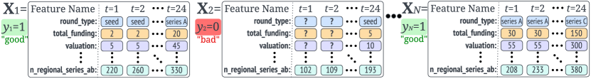
Figure 1. An illustration of multivariate time series dataset ($N$ samples) to train models for VC and GC sourcing.

3. The Approach

Our approach tackles the problem of identifying good investment targets for VC and GC by framing it as a multivariate time series classification task. Specifically, each potential investment target (i.e. candidate company) is represented by a multivariate time series $\mathbf{X}\in\mathbb{R}^{T\times K}$, as shown in Figure 1. $\mathbf{X}$ consists of $T$ observations, each containing $K$ variables that describe different aspects (e.g., funding, revenue, etc.) of the corresponding company. Formally, each sample $\mathbf{X}$ is a sequence of $T$ feature vectors: $\mathbf{X}\!=\![\mathbf{x}_{1},\mathbf{x}_{2},\ldots,\mathbf{x}_{t},\ldots,\mathbf{x}_{T}]$, where $\mathbf{x}_{t}\!\in\!\mathbb{R}^{K}$. At each time step $t$, we collect $K$ numerical or categorical features about the company to form the vector $\mathbf{x}_{t}$, which captures a multi-view snapshot of the company at that time point. The last vector $\mathbf{x}_{T}$ represents the most recent state of the company. Depending on the data available, the time interval between two adjacent time points, $t$ and $t+1$, can be set to a month, a quarter, or any other length of choice. By adopting this representation, we can model a multi-view evolution of each company over time and make informed predictions about their future success.

We assume that we have collected a set of $N$ samples, each corresponding to a different company, denoted by ${\mathbf{X}_{1},\mathbf{X}_{2},\ldots,\mathbf{X}_{n},\ldots,\mathbf{X}_{N}}$. For each sample $\mathbf{X}_{n}$, we have a binary ground truth label $y_{n}\!\in\!\{0,1\}$ indicating a “bad” or “good” investment target according to some criteria. Details of how we define and collect these labels are explained in Section 3.3. We construct a dataset $\mathfrak{U}$ from these samples and labels as $\mathfrak{U}=\{(\mathbf{X}_{1},y_{1}),(\mathbf{X}_{2},y_{2}),\ldots,(\mathbf{X}_{N},y_{N})\}$, where $n\in\mathbb{Z}\cap[1,N]$. Our objective then is to train a model on $\mathfrak{U}$ to accurately predict the ground truth labels $y_{n}$ using $\mathbf{X}_{n}$. We use $\hat{y}_{n}\in[0,1]$ to denote the predicted probability of future success of the company represented by $\mathbf{X}_{n}$, in order to distinguish it from the ground truth label $y_{n}$. For the sake of brevity, we use general terms $\mathbf{X}$, $y$, and $\hat{y}$ to denote $\mathbf{X}_{n}$, $y_{n}$, and $\hat{y}_{n}$, respectively.

3.1. Time Series Features

We define the input time series features $\mathbf{X}$ by constructing 16 time series that fall into 6 feature categories, as summarized in (Cao et al., 2022b). These categories are funding, founder/owner, team, investor, web, and context, and below we will introduce the selected features under each category. Each time series feature contains precisely $T$ values corresponding to the $T$ time steps. For a concrete example of $\mathbf{X}$, see Figure 1. All time series features are numerical, with the exception of the first one (round_type), which is categorical. Each time step corresponds to a calendar month, and the steps are aligned monthly. For further details regarding time series padding, imputation and scaling, please refer to Section 4.1.

Funding: this category contains statistics of historical funding received by the company, indicating recognition from investors.

• round_type indicates the latest funding round type that a company has received up to time $t$, such as Seed or Series A, thus providing insights into its funding stage and maturity.

• total_funding is the cumulative amount of funding in USD that the company has received up to time $t$, indicating the amount of capital it has been able to attract.

• valuation: the estimated USD valuation of the company immediately following its latest funding round and is included to provide insight into a company’s overall financial value.

Founder/Owner: this category captures attributes of the founding team, which are critical to a company’s short-term success and long-term survival (Ghassemi et al., 2020).

• n_founder shows the number of a company’s founders still with the company at time $t$.

Team: complementary to the founder/owner feature, this category captures the statistics of the employees of the company.

• n_employee: the number of employees working for the company at time $t$, implying the company’s growth trajectory.

Investor category captures the investor-level statistics (as opposed to the company-level funding statistics above) for investors who have funded the company, indicating its early attractiveness.

• n_investor represents the total number of unique investors who have provided funding to the company up to time $t$. This feature provides insights into the diversification of the company’s investment sources.

• growth_investor_rate is the ratio of unique GC investors among the company’s unique investors up to time $t$. This feature indicates the investors’ beliefs in the company’s future growth potential.

• average_cagr is the average Compound Annual Growth Rate (CAGR) of all exited deals made by the company’s investors up to time $t$. This feature is meant to demonstrate the past investment performance of the involved investors.

• 2x_cagr_rate is calculated as the ratio of investment deals up to time $t$ with a CAGR$\geq$2 among all exited deals made by the company’s investors. This feature reflects the proportion of investors with a history of impressive returns who are currently invested in the company.

Web: this category covers any feature extracted from web pages that are related to the company in focus.

• cu_popularity describes the company’s domain name popularity rank at time $t$ . This rank is determined based on the domain’s network traffic as measured by Cisco Umbrella (CU).

• sw_global_rank describes at time $t$ the monthly unique visitors and pageviews of the company website(s). This feature is obtained from SimilarWeb.

• n_desktop_visitor and n_mobile_visitor are two features indicating the number of unique visitors to the company’s website utilizing a desktop and mobile device, respectively. Both of these features are sourced from SimilarWeb.

• n_news counts the number of times a company is mentioned across approximately 3,700 news websites up till a certain time point $t$, reflecting its media visibility and recognition.

Context: this category captures extrinsic factors that may be (but are not limited to) competition, regional, environmental, cultural, economical or tax based.

• n_regional_seed_round represents the number of seed funding rounds in the company’s region between adjacent time points $t\!-\!1$ and $t$. This feature offers context on the company’s performance relative to regional competitors and financial conditions, highlighting potential company success even if regional investments are low.

• n_regional_series_ab: similar to the previous feature except that it is counting the Series A and B rounds instead.

It should be noted the features above are by no means exhaustive. If available, additional features could be incorporated, describing for example market conditions, company financial performance, leadership team composition, or more granular employee hiring and churn patterns. Additionally, there is wide potential to expand the contextual features evaluated in this study. For example, many of the non-contextual features introduced above could be contextualized with regard to a company’s region, market, growth stage, industry, or competitors. We leave this work for future research.

3.2. TMTSC Architecture

As illustrated in Figure 2, TMTSC learns to predict $\hat{y}_{n}$ using input $\mathbf{X}=[\mathbf{x}_{1},\mathbf{x}_{2},\ldots,\mathbf{x}_{t},\ldots,\mathbf{x}_{T}]$. At the $t$-th time step, each input feature vector $\mathbf{x}_{t}$ consists of a numerical part (often normalized), denoted as $\mathbf{u}_{t}$, and a categorical part, denoted as $\mathbf{v}_{t}$. Thus, $\mathbf{x}_{t}=[\mathbf{u}_{t};\mathbf{v}_{t}]$, where “;” represents a vector concatenation operation. To convert the categorical features $\mathbf{v}_{t}$ into dense embeddings, we utilize embedding layers, which can be collectively represented by a learnable function $\mathcal{E}$. The embedded categorical features are then given by $\mathbf{v}^{\prime}_{t}=\mathcal{E}(\mathbf{v}_{t})$. As a result, the $K$-dimensional vector $\mathbf{x}_{t}$ is transformed to a new numerical vector $\mathbf{x}^{\prime}_{t}$ that has $K^{\prime}$ ($K^{\prime}>K$) dimensions:

(1) $$\mathbf{x}^{\prime}_{t}=[\mathbf{u}_{t};\mathcal{E}(\mathbf{v}_{t})]\in\mathbb{R}^{K^{\prime}}\;\text{and }\;\mathbf{x}_{t}=[\mathbf{u}_{t};\mathbf{v}_{t}]\in\mathbb{R}^{K}.$$

Then, $\mathbf{x}^{\prime}_{t}$ is linearly projected onto a $D$-dimensional vector space, where $D$ is the dimension of the Transformer model sequence element representations, a.k.a. model dimension:

(2) $$\mathbf{h}_{t}=\mathbf{W}\mathbf{x}^{\prime}_{t}+\mathbf{b},$$

where $\mathbf{W}\in\mathbb{R}^{D\times K^{\prime}}$ and $\mathbf{b}\in\mathbb{R}^{D}$ are learnable parameters and $\mathbf{h}_{t}\in\mathbb{R}^{D}$, $t\in\mathbb{Z}\cap[1,T]$ are the input vectors to the Transformer model. Although Equation (1) and (2) show the operation for a single time step for clarity, all raw input vectors $\mathbf{x}_{t}$, $t\in\mathbb{Z}\cap[1,T]$ are embedded in the same way concurrently. It is worth mentioning that the above formulation can also accommodate the case of univariate time series (i.e., $K=1$), though in the scope of this work, we will only evaluate the approach on multivariate time series.

It is important to note that the Transformer is a feed-forward architecture that does not inherently account for the order of input elements. To address the sequential nature of time series data, we incorporate positional encodings, denoted as $\mathbf{P}=[\mathbf{p}_{1},\mathbf{p}_{2},\ldots,\mathbf{p}_{T}]\in\mathbb{R}^{T\times D}$, to the input vectors $\mathbf{H}=[\mathbf{h}_{1},\mathbf{h}_{2},\ldots,\mathbf{h}_{T}]\in\mathbb{R}^{T\times D}$, resulting in the final input $\mathbf{H}^{\prime}$:

(3) $$\mathbf{H}^{\prime}=\mathbf{H}+\mathbf{P}=[\mathbf{h}^{\prime}_{1},\mathbf{h}^{\prime}_{2},\ldots,\mathbf{h}^{\prime}_{T}]\in\mathbb{R}^{T\times D},$$

where $\mathbf{h}^{\prime}_{t}\in\mathbb{R}^{D}=\mathbf{h}_{t}+\mathbf{p}_{t}$. Closely following the approach in (Zerveas et al., 2021), we employ fully learnable positional encodings, as they have been reported to yield better performance compared to deterministic sinusoidal encodings (Vaswani et al., 2017) for multivariate time series classification tasks. We also utilize batch normalization (rather than layer normalization), as it is considered effective in mitigating the impact of outlier values in time series data, an issue that does not typically arise for textual inputs.

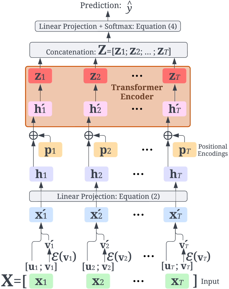
Figure 2. The illustration of TMTSC model architecture.

The Transformer-based model architecture depicted in Figure 2 generates $T$ output vectors $z_{t}$ corresponding to the $T$ input time steps. These output vectors are concatenated to form a single output matrix $\mathbf{Z}=[\mathbf{z}_{1};\mathbf{z}_{2};\ldots;\mathbf{z}_{T}]$, which serves as the input for a linear layer. As shown in Equation (4), the linear layer is parameterized by $\mathbf{W}_{\text{out}}\in\mathbb{R}^{C\times(T\cdot D)}$ and $\mathbf{b}_{\text{out}}\in\mathbb{R}^{C}$, where $C$ denotes the number of classes to be predicted.

(4) $$\hat{\mathbf{y}}=\text{\it Softmax}(\mathbf{W}_{\text{out}}\mathbf{Z}+\mathbf{b}_{\text{out}})\in\mathbb{R}^{C},$$

where $\text{\it Softmax}(\cdot)$ is a softmax function for obtaining a probability distribution over classes.

3.3. Optimization Target

In the absence of a universally agreed-upon definition of “true success” of startups and scaleups, most existing definitions tend to focus on “growth”, which can be measured from various perspectives, such as funding, revenue, employee count, and valuation, among others (Cao et al., 2022b). As a well-established investment firm, we have access to a large volume of expert evaluations (akin to (Bai and Zhao, 2021; Kinne and Lenz, 2021)) that represent quantified assessments from human experts. These evaluations encompass multiple categories/terms, such as “inbound”, “reviewing”, “reach-out”, “follow”, “negotiating”, and “out-of-scope”, which are updated periodically by investment professionals for companies in the context of VC and GC. To further simplify the prediction task, we assign each evaluation term to either a good (“1”) or bad (“0”) binary bucket denoted by $\mathbf{y}_{n}$ in Figure 1, implying $C$=2 in Equation (5). In this way, each company is annotated with two ground-truth binary labels – one for VC and the other for GC; and the loss function $\mathcal{L}$ is defined as

(5) $$\mathcal{L}=-\frac{1}{N}\sum_{n=1}^{N}\left[\mathbf{y}_{n}\log(\hat{\mathbf{y}}_{n})+(1-\mathbf{y}_{n})\log(1-\hat{\mathbf{y}}_{n})\right].$$

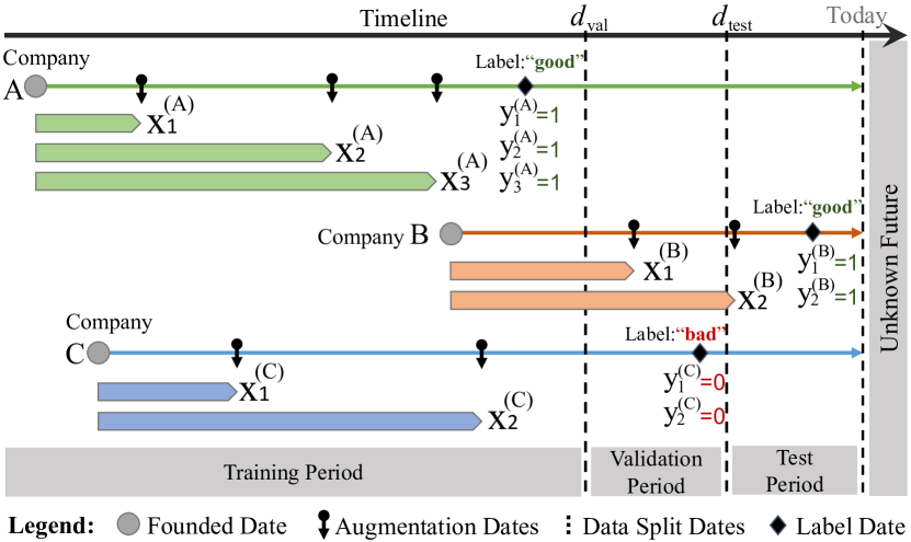
Figure 3. Visualization (adapted from (Cao et al., 2022b)) of investor-centric data augmentation and split using three example companies.

3.4. Investor-Centric Augmentation and Split

The standard practice for ML and DL approaches involves dividing the entire dataset into non-overlapping training, validation, and test subsets. Various models are trained using different sets of hyper-parameters solely on the training subset. The optimal model is chosen based on the evaluation metrics obtained on the validation subset. The test set is then utilized to assess the generalization performance of the selected model prior to deployment. In this work, we adopt the so-called investor-centric strategy (Wu et al., 2022; Ferrati et al., 2021), because it better resembles the real-world scenario of how investment professionals predict the success of companies (Cao et al., 2022b). The main idea behind this strategy consists of two consecutive steps: a company augmentation step followed by a sample split step. To facilitate our discussion, we present a minimal example in Figure 3, which features three companies (A, B, and C) founded at different dates along the timeline. Based on investment professionals’ evaluations (Section 3.3), companies A and B are labeled as positive (i.e., promising investing targets: $\small\smash{\mathbf{y}^{(\text{A})}\!\!=\!\mathbf{y}^{(\text{B})}\!\!=\!1}$) sometime after their establishment. On the other hand, some companies might be annotated negatively (e.g., company C with label $\small\smash{\mathbf{y}^{(\text{C})}\!\!=\!0}$) by VC/GC experts if they show no signs of success within a few years after their founding dates.

During the company augmentation step, one can randomly or heuristically sample several dates before the corresponding label date; these dates are referred to as augmentation dates. Consequently, we can compute one sample using data prior to each augmentation date. As illustrated in Figure 3, there are three augmentation dates on the timeline of company A, resulting in three samples (i.e., $\small\smash{\mathbf{X}_{1}^{(\text{A})}}$, $\small\smash{\mathbf{X}_{2}^{(\text{A})}}$ and $\small\smash{\mathbf{X}_{3}^{(\text{A})}}$) that are all labeled as positive samples (i.e., $\small\smash{\mathbf{y}_{1}^{(\text{A})}\!\!=\!\mathbf{y}_{2}^{(\text{A})}\!\!=\!\mathbf{y}_{3}^{(\text{A})}\!\!=\!1}$). In a sense, company A is augmented by generating three $\langle$sample, label$\rangle$ pairs: $\small\smash{\langle\mathbf{X}_{1}^{(\text{A})}\!\!,\mathbf{y}_{1}^{(\text{A})}\rangle}$, $\small\smash{\langle\mathbf{X}_{2}^{(\text{A})}\!\!,\mathbf{y}_{2}^{(\text{A})}\rangle}$ and $\small\smash{\langle\mathbf{X}_{3}^{(\text{A})}\!\!,\mathbf{y}_{3}^{(\text{A})}\rangle}$. Similarly, B and C create another four pairs: $\small\smash{\langle\mathbf{X}_{1}^{(\text{B})}\!\!,\mathbf{y}_{1}^{(\text{B})}\rangle}$, $\small\smash{\langle\mathbf{X}_{2}^{(\text{B})}\!\!,\mathbf{y}_{2}^{(\text{B})}\rangle}$, $\small\smash{\langle\mathbf{X}_{1}^{(\text{C})}\!\!,\mathbf{y}_{1}^{(\text{C})}\rangle}$ and $\small\smash{\langle\mathbf{X}_{2}^{(\text{C})}\!\!,\mathbf{y}_{2}^{(\text{C})}\rangle}$. In this example, three companies are augmented into seven samples in total. The decision about how much augmentation to undertake should be informed by the time granularity of the data available. For example, if working with monthly data, augmenting on a weekly basis will simply duplicate data without providing any additional information for a model.

In the sample split step, the global timeline is divided into three periods: training (from the earliest founding date to $d_{\text{val}}$), validation (from $d_{\text{val}}$ to $d_{\text{test}}$), and testing (from $d_{\text{test}}$ to “today”), as depicted in Figure 3. The period to which a company’s label belongs determines the dataset split it should be assigned to. Following this rule, we can infer from Figure 3 that the three $\langle$sample, label$\rangle$ pairs from company A should be allocated to the training set, the two pairs from company B to the test set, and the two pairs from company C to the validation set. The selection of the two splitting dates, $d_{\text{val}}$ and $d_{\text{test}}$, aims to closely approximate the target train:val:test split ratio of 8:1:1. Achieving this ratio split exactly is not feasible because (1) the dataset is divided along the time axis, and (2) all samples from the same company must belong to the same subset to avoid data leakage. Therefore, we search for the optimal splitting dates using a grid search strategy, iterating through different combinations of discrete $d_{\text{val}}$ and $d_{\text{test}}$ values.

Dataset	#feat.	#sample	#time step	#class	#train	#val.	#test
Ethanol	3	524	1751	4	261	-	263
PEMS-SF	963	440	144	7	267	-	173
VC	16	86,886	24	2	63,562	11,178	12,146
GC	16	21,163	24	2	16,275	-	4,888

Table 1. Specification of benchmarking datasets/tasks.

4. Experiments

To evaluate the performance of TMTSC, we experiment four baseline methods on four datasets/tasks (2 proprietary + 2 public).

4.1. Benchmarking Datasets

Following the procedure introduced in Sections 3.1, 3.3 and 3.4, we prepare two proprietary datasets: “VC” for the VC context and “GC” for the GC context, performing data augmentation to obtain monthly time steps. To eliminate overly sparse time series, we discard the samples whose time series features are all shorter than six months. Missing valuation values are approximated with the cumulative funding received up to that point. Missing total_funding values are filled by taking the value of the previous month (if available) or 0 otherwise. For the time steps where the values are still missing, we fill them with “-1”. Finally, we pad all time series to the same length of 24 months. As for scaling, we empirically apply log-transform to 13 numerical features (excluding cu_popularity and n_employee).

To gain a more complete view of our experimental results, we also include two public TSC (time series classification) benchmark datasets: Ethanol (Large et al., 2018) and PEMS-SF (Cuturi, 2011). We adopt the Min-Max normalization and the default data splits. The specifications of the benchmarking datasets is presented in Table 1.

4.2. Compared Baselines

GRU (Gated Recurrent Unit) (Chung et al., 2014) is a highly relevant baseline for comparison due to its ability to model sequential dependencies and capture long-term dependencies in time series data. We experiment both U-GRU (Univariate GRU) and M-GRU (Multivariate GRU), whose architectures are illustrated in Figure 4 and 5 respectively. We adopt the implementation of BiGRU (Bidirectional GRU) (Cho et al., 2014), masking, embedding, dropout, and dense layers from Keras. In both architectures, the masking layer is added to inform the model to ignore any values marked as missing in its computation.

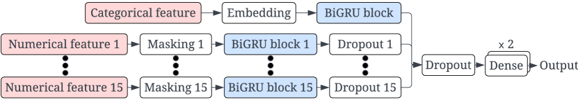
Figure 4. U-GRU architecture: each univariate time series feature is modeled by an individual BiGRU block.

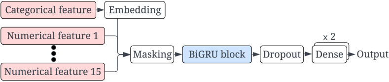
Figure 5. M-GRU architecture: all time series features are modeled by one single BiGRU block.

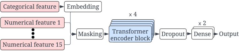
Figure 6. TE architecture with 4 Transformer encoder blocks.

Taking advantage of the popular Transformer architecture, employing transformer-based TSCs for benchmarking enables access to state-of-the-art performance, ensuring robust modeling of temporal dynamics. Inspired by (Zerveas et al., 2021), we introduce TMTSC in Section 3.2 to address the VC/GC sourcing problem in the form of TSC. As a close relative and foundation of TMTSC, the Transformer Encoder (TE) (Vaswani et al., 2017) is also selected as a baseline. As shown in Figure 6, we adopt the same layers as the original implementation (Vaswani et al., 2017). For the sake of comparability, the input features are ingested, embedded and concatenated in the same way as M-GRU as shown in Figure 5.

Hyper-parameter	M-GRU	U-GRU
Batch Size	128, 256, 512	512
Learning Rate	0.0001, 0.001	0.0002
Optimizer	Adam, RMSProp	Adam
Normalizer	Z-Scoring, Min-Max	Z-Scoring
Top-$K$ Round Types	15, 25, 35	25
# Dimension of Embedding Layer	3, 5, 10	3
GRU Units	32, 64, 128, 256	32
# Units of Dense Layer	32, 64, 128, 256	32
Dropout Rate	0.0, 0.2, 0.3, 0.5	0.2

Table 2. Hyper-parameters for U-GRU and M-GRU baselines.

Parameter	TE	TMTSC
Learning Rate	0.0001, 0.001	0.0001, 0.001
Optimizer	Adam, RMSProp	Adam, RAdam (Liu et al., 2020)
Normalizer	Z-Scoring, Min-Max	Z-Scoring, Min-Max
Attention Dimensions	128, 256, 512	64, 128, 256
# Transformer Heads	4, 8	4, 8 16, 32
# Transformer Blocks	4, 6	2, 3, 4
# Units of Dense Layer	128, 256	256, 512
Dropout Rate	0, 0.2, 0.4	0.1, 0.2, 0.3
Normalisation Layer	Layer Norm.	Layer, Batch Norm.
Activation	ReLu	ReLu, GeLu (Hendrycks and Gimpel, 2016)
# Convolutional Filters	4, 8	-
L2 Regularization	-	0, 0.2, 0.3

Table 3. Hyper-parameters for TMTSC and TE baselines.

4.3. Hyper-Parameter Selection

The hyper-parameters were selected based on the highest AUC-ROC (“Area Under the Curve” of the Receiver Operating Characteristic curve) score on the validation split of the VC dataset. The selected hyper-parameters are also applied to GC dataset due to similar input format and dataset scale. For Ethanol or PEMS-SF datasets, we either reuse the hyper-parameters in (Zerveas et al., 2021) or search for the best combination on the pre-defined test split. Since U-GRU resembles a substructure of one of our deployed models, we simply adopt the hyper-parameter values from the training pipeline of that model. Table 2 and 3 present the searched and selected (in bold) values of hyper-parameters for each baseline models, where “Top-$K$ Round Types” indicates that only the most common $K$ round types were kept for the categorical round_type feature.

Dataset	Metric	U-GRU	M-GRU	TE	TMTSC
Ethanol (public)	Accuracy $\pm$STDEV	0.358 $\pm$0.038	0.364 $\pm$0.011	0.327 $\pm$0.029	0.337* $\pm$N/A*
PEMS-SF (public)	Accuracy $\pm$STDEV	N/A$\dagger$ $\pm$N/A$\dagger$	0.722 $\pm$0.019	0.234 $\pm$0.057	0.919* $\pm$N/A*
VC (proprietary)	Accuracy $\pm$STDEV	0.548 $\pm$0.013	0.731 $\pm$0.026	0.655 $\pm$0.081	0.863 $\pm$0.015
	Precision $\pm$STDEV	0.704 $\pm$0.015	0.740 $\pm$0.044	0.699 $\pm$0.062	0.864 $\pm$0.016
	AUC-ROC $\pm$STDEV	0.628 $\pm$0.015	0.819 $\pm$0.020	0.780 $\pm$0.081	0.924 $\pm$0.009
GC (proprietary)	Accuracy $\pm$STDEV	0.934 $\pm$0.011	0.924 $\pm$0.027	0.933 $\pm$0.021	0.956 $\pm$0.004
	Precision $\pm$STDEV	0.701 $\pm$0.058	0.794 $\pm$0.101	0.765 $\pm$0.108	0.831 $\pm$0.026
	AUC-ROC $\pm$STDEV	0.977 $\pm$0.008	0.939 $\pm$0.002	0.971 $\pm$0.002	0.971 $\pm$0.001

* Results are cited from (Zerveas et al., 2021), and the STDEV is not available or calculable.

$\dagger$ Not available due to exceeding the limitation of computational constraints.

Table 4. Performance comparison on four datasets. Results are reported over 3 runs and the best results are in bold.

4.4. Overall Performance

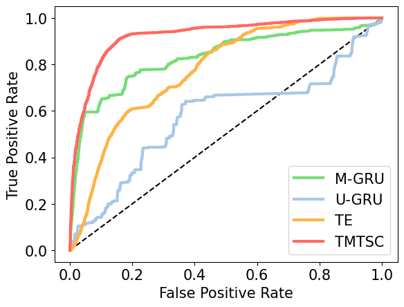
(a) VC dataset

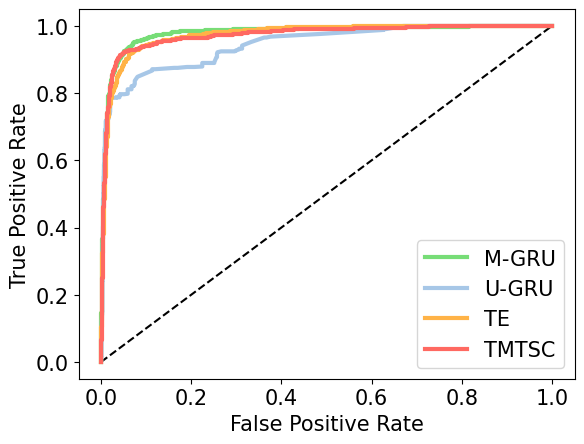
(b) GC dataset

Figure 7. ROC (Receiver Operating Characteristic) curves.

As indicated in Table 4, No major discrepancies can be seen in the public Ethanol dataset when comparing the different architectures. This is likely attributed to the inherent nature of this dataset: many classes and few samples. The PEMS-SF dataset reveals a large disparity among the compared methods. TMTSC achieves a remarkable 74.5% increase in accuracy compared to TE, indicating that learning on high-dimensional datasets is difficult due to the lack of positional encoding. TMTSC also surpasses the second best architecture (M-GRU) due to its multi-head attention modules, which are advantageous in dealing with high-dimensional temporal data.

When it comes to evaluating the two proprietary datasets, the costs of different types of prediction errors must be considered. The outcome from false negatives (failing to identify a successful company) is that investors are simply not made aware of a successful company and therefore no action is taken. In that regard, there is an upside loss in terms of lost profit but no detriment in terms of time or money invested. False positives (incorrectly predicting a company will be successful), on the other hand, can lead to wasted time spent on due diligence, or, in the worst case, an investment that loses money. For that reason, it is more important to evaluate a model with respect to its precision, or the number of its positive predictions that are actually positive. Observing the precision scores in Table 4, TMTSC outperforms all other methods, achieving scores of 0.86 and 0.83 for VC and GC scenario, respectively.

Additionally, Figure 7 tries to provide a more balanced and comprehensive view using AUC-ROC metic. TMTSC clearly outperforms on the VC dataset, achieving an average score of 0.92, 12% better than M-GRU, the next best method. All methods performed extremely well on the GC dataset, and TMTSC’s AUC-ROC score of 0.97 is less than 1% lower than the winner U-GRU.

4.5. Training Stability and Efficiency

The standard deviation values (STDEV) in Table 4 indicate that the TMTSC training is relatively stable in both the VC and GC datasets, as the values are relatively low compared to the other baselines. To measure training efficiency, we record per-step training time for each dataset and method using the same batch size (=512) and hardware configurations. The results are presented in Table 5, where the “Relative Time” column shows how the time consumption for the corresponding method relates to the fastest method (i.e., “1.0 $\times$”). Take the VC task for example, “2.4 $\times$” for TE would therefore mean TE took over twice as long as M-GRU. It is evident that M-GRU requires the least amount of training time, largely due to its design, which favors simplicity. TMTSC and TE take only a small amount of extra time to train, despite their increased complexity. This is likely because of their multi-head architecture, which allows for parallelization of self-attention computations.

Dataset	Method	Sec./Step	Relative Time
VC	U-GRU	2.000	83.3 $\times$
	M-GRU	0.024	1.0 $\times$
	TE	0.057	2.4 $\times$
	TMTSC	0.100	4.2 $\times$
GC	U-GRU	1.232	46.6 $\times$
	M-GRU	0.026	1.0 $\times$
	TE	0.056	2.1 $\times$
	TMTSC	0.101	3.8 $\times$

Table 5. The comparison of training efficiency. Underlined values indicate shortest time per step for each dataset.

4.6. Portfolio Simulation

To further evaluate the model in the context of the real-world investment scenario, portfolio simulations are executed and visualized in Figure 8. Concretely, we assemble a set by isolating the companies confirmed to be potentially good investment targets in the VC or GC datasets (i.e., that are positively labeled). From this set, we randomly sample $i$ companies to simulate forming VC/GC investment portfolios of size $i$ and calculate the percentage of companies each model predicts to be successful within the sample. To address the stochasticity of this process, we perform each simulation 100 times. Different portfolio sizes (i.e., values of $i$) are simulated; and for each $i$ (X-axis), the mean and standard deviations are plotted (Y-axis), resulting in a colored line with a shaded area in Figure 8.

In VC and GC contexts, we can see that (1) TMTSC performs the best among all methods, (2) performance becomes less variable as simulated portfolio size increases, and (3) the models evaluated performed more variably on the VC dataset than the GC dataset.

To roughly compare these methods against real-world VC and GC fund performance, Figure 8(a), includes the portfolio size and performance of five VC funds (Yin et al., 2021) , showing a performance largely on par with M-GRU and inferior to TMTSC and TE. For the GC simulation, a horizontal line representing the real-world GC success rate of 86.3% (Mooradian et al., 2019) is included in Figure 8(a) . Here, the real-world GC success rate is outperformed by M-GRU and TMTSC. It is important to note that investment firms are much more constrained than the simulation: they cannot invest in every attractive company they encounter due to factors like founders’ preference, portfolio conflict, investment focus, and available funds.

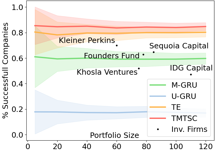
(a) VC dataset

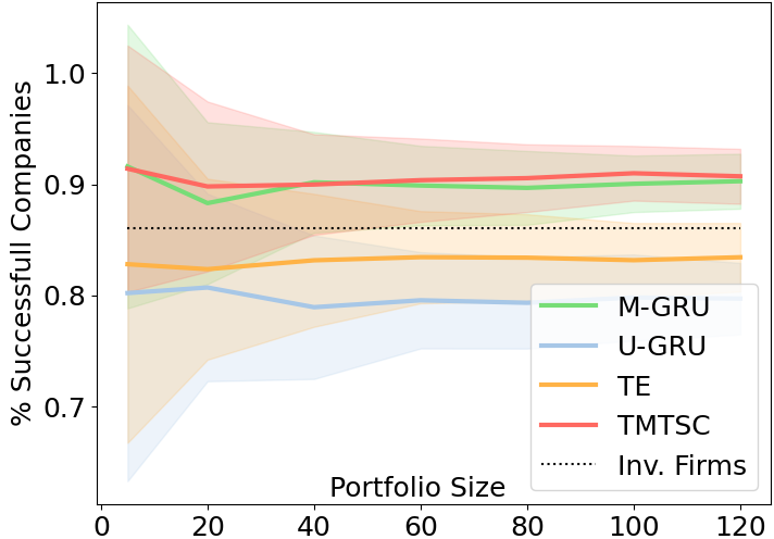
(b) GC dataset

Figure 8. Portfolio simulation: success rate vs. portfolio size.

5. Conclusion and Future Work

In this work, we propose using a Transformer-based Multivariate Time Series Classifier (TMTSC) to facilitate sourcing investment targets for Venture Capital (VC) and Growth Capital (GC). Specifically, TMTSC utilizes multivariate time series as input to predict the probability that any candidate company will succeed in the context of a VC or GC fund. We formally define the sourcing problem as a multivariate time series classification task, and introduce the key components of our implementation, including input features, model architecture, optimization target, and investor-centric data augmentation and split. We experimentally validate the superior accuracies obtained by TMTSC model on two public multivariate time series datasets. More importantly, our extensive experiments on two proprietary datasets (collected from VC and GC contexts) demonstrate the effectiveness, stability, and efficiency of our approach compared with three popular baselines. To further evaluate the model in the context of the real-world investment scenario, portfolio simulations are executed, showing TMTSC’s high success rate in both VC and GC sourcing. The main future work includes (1) incorporating global features along with time series input, (2) and learning generic and condensed representations for multivariate time series for varies downstream prediction tasks.

- (1)
- Allu and Padmanabhuni (2022) Ramakrishna Allu and Venkata Nageswara Rao Padmanabhuni. 2022. Predicting the success rate of a start-up using LSTM with a swish activation function. Journal of Control and Decision 9, 3 (2022), 355–363.
- Ang et al. (2022) Yu Qian Ang, Andrew Chia, and Soroush Saghafian. 2022. Using machine learning to demystify startups’ funding, post-money valuation, and success. In Innovative Technology at the Interface of Finance and Operations. Springer, 271–296.
- Arroyo et al. (2019) Javier Arroyo, Francesco Corea, Guillermo Jimenez-Diaz, and Juan A Recio-Garcia. 2019. Assessment of machine learning performance for decision support in venture capital investments. IEEE Access 7 (2019), 124233–124243.
- Bai and Zhao (2021) Sarah Bai and Yijun Zhao. 2021. Startup Investment Decision Support: Application of Venture Capital Scorecards Using Machine Learning Approaches. Systems 9, 3 (2021), 55.
- Blank (2013) Steve Blank. 2013. Why the lean start-up changes everything. Harvard business review 91, 5 (2013), 63–72.
- Block et al. (2019) Joern Block, Christian Fisch, Silvio Vismara, and René Andres. 2019. PE investment criteria: An experimental conjoint analysis of venture capital, business angels, and family offices. Journal of Corporate Finance 58 (2019), 329–352.
- Bonaventura et al. (2020) Moreno Bonaventura, Valerio Ciotti, Pietro Panzarasa, Silvia Liverani, Lucas Lacasa, and Vito Latora. 2020. Predicting success in the worldwide start-up network. Scientific Reports 10, 1 (2020), 1–6.
- Cao et al. (2022a) Lele Cao, Sonja Horn, Vilhelm von Ehrenheim, Richard Anselmo Stahl, and Henrik Landgren. 2022a. Simulation-Informed Revenue Extrapolation with Confidence Estimate for Scaleup Companies Using Scarce Time Series Data. In Proceedings of the 31st ACM International Conference on Information and Knowledge Management (CIKM ’22), October 17–21, 2022, Atlanta, GA, USA. Association for Computing Machinery (ACM), New York, NY, USA, 12 pages.
- Cao et al. (2023) Lele Cao, Vilhelm von Ehrenheim, Astrid Berghult, Henje Cecilia, Richard Anselmo Stahl, Joar Wandborg, Sebastian Stan, Armin Catovic, Erik Ferm, and Ingelhag Hannes. 2023. A Scalable and Adaptive System to Infer the Industry Sectors of Companies: Prompt + Model Tuning of Generative Language Models. In Proceedings of the IJCAI Workshop on Financial Technology And Natural Language Processing (FinNLP). 1–11.
- Cao et al. (2022b) Lele Cao, Vilhelm von Ehrenheim, Sebastian Krakowski, Xiaoxue Li, and Alexandra Lutz. 2022b. Using Deep Learning to Find the Next Unicorn: A Practical Synthesis. arXiv preprint arXiv:2210.14195 (2022).
- Cavallo et al. (2019) Angelo Cavallo, Antonio Ghezzi, Claudio Dell’Era, and Elena Pellizzoni. 2019. Fostering digital entrepreneurship from startup to scaleup: The role of venture capital funds and angel groups. Technological Forecasting and Social Change 145 (2019), 24–35.
- Chen et al. (2021) Miao Chen, Chao Wang, Chuan Qin, Tong Xu, Jianhui Ma, Enhong Chen, and Hui Xiong. 2021. A Trend-aware Investment Target Recommendation System with Heterogeneous Graph. In Intl. Joint Conf. on Neural Networks. 1–8.
- Cheng et al. (2019) Chaoran Cheng, Fei Tan, Xiurui Hou, and Zhi Wei. 2019. Success Prediction on Crowdfunding with Multimodal Deep Learning.. In International Joint Conference on Artificial Intelligence. 2158–2164.
- Chernenko et al. (2021) Sergey Chernenko, Josh Lerner, and Yao Zeng. 2021. Mutual funds as venture capitalists? Evidence from unicorns. The Review of Financial Studies 34, 5 (2021), 2362–2410.
- Cho et al. (2014) Kyunghyun Cho, Bart van Merriënboer, Caglar Gulcehre, Dzmitry Bahdanau, Fethi Bougares, Holger Schwenk, and Yoshua Bengio. 2014. Learning Phrase Representations using RNN Encoder–Decoder for Statistical Machine Translation. In Proceedings of the Conference on Empirical Methods in Natural Language Processing (EMNLP). Association for Computational Linguistics, Doha, Qatar, 1724–1734.
- Chung et al. (2014) Junyoung Chung, Caglar Gulcehre, Kyunghyun Cho, and Yoshua Bengio. 2014. Empirical evaluation of gated recurrent neural networks on sequence modeling. In NIPS 2014 Workshop on Deep Learning, December 2014.
- Cuturi (2011) Marco Cuturi. 2011. Fast global alignment kernels. In Proceedings of the 28th international conference on machine learning (ICML-11). 929–936.
- Dellermann et al. (2021) Dominik Dellermann, Nikolaus Lipusch, Philipp Ebel, Karl Michael Popp, and Jan Marco Leimeister. 2021. Finding the unicorn: Predicting early stage startup success through a hybrid intelligence method. In International Conference on Information Systems.
- Ferrati et al. (2021) Francesco Ferrati, Haiquan Chen, and Moreno Muffatto. 2021. A Deep Learning Model for Startups Evaluation Using Time Series Analysis. In European Conf. on Innovation and Entrepreneurship. Academic Conferences limited, 311.
- Garkavenko et al. (2022) Mariia Garkavenko, Eric Gaussier, Hamid Mirisaee, Cédric Lagnier, and Agnès Guerraz. 2022. Where Do You Want To Invest? Predicting Startup Funding From Freely, Publicly Available Web Info. arXiv:2204.06479 (2022).
- Gastaud et al. (2019) Clement Gastaud, Theophile Carniel, and Jean-Michel Dalle. 2019. The varying importance of extrinsic factors in the success of startup fundraising: competition at early-stage and networks at growth-stage. arXiv:1906.03210 (2019).
- Ghassemi et al. (2020) M Ghassemi, C Song, and T Alhanai. 2020. The Automated Venture Capitalist: Data and Methods to Predict the Fate of Startup Ventures. In AAAI Workshop on Knowledge Discovery from Unstructured Data in Financial Services.
- Gompers et al. (2020) Paul A Gompers, Will Gornall, Steven N Kaplan, and Ilya A Strebulaev. 2020. How do venture capitalists make decisions? Journal of Financial Economics 135, 1 (2020), 169–190.
- Goodfellow et al. (2016) Ian Goodfellow, Yoshua Bengio, and Aaron Courville. 2016. Deep learning. MIT press.
- Guerzoni et al. (2019) Marco Guerzoni, Consuelo R Nava, and Massimiliano Nuccio. 2019. The survival of start-ups in time of crisis. a machine learning approach to measure innovation. arXiv preprint arXiv:1911.01073 (2019).
- Hendrycks and Gimpel (2016) Dan Hendrycks and Kevin Gimpel. 2016. Gaussian error linear units (gelus). arXiv preprint arXiv:1606.08415 (2016).
- Horn (2021) Sonja Horn. 2021. Deep learning models as decision support in venture capital investments: Temporal representations in employee growth forecasting of startup companies. Master’s thesis. KTH Royal Institute of Technology & EQT Partners.
- Kaiser and Kuhn (2020) Ulrich Kaiser and Johan M Kuhn. 2020. The value of publicly available, textual and non-textual information for startup performance prediction. Journal of Business Venturing Insights 14 (2020), e00179.
- Kinne and Lenz (2021) Jan Kinne and David Lenz. 2021. Predicting innovative firms using web mining and deep learning. PloS One 16, 4 (2021), e0249071.
- Krishna et al. (2016) Amar Krishna, Ankit Agrawal, and Alok Choudhary. 2016. Predicting the outcome of startups: less failure, more success. In International Conference on Data Mining Workshop. 798–805.
- Large et al. (2018) James Large, E Kate Kemsley, Nikolaus Wellner, Ian Goodall, and Anthony Bagnall. 2018. Detecting Forged Alcohol Non-invasively Through Vibrational Spectroscopy and Machine Learning. In Pacific-Asia Conference on Knowledge Discovery and Data Mining. Springer, 298–309.
- Liang and Yuan (2016) Yuxian Eugene Liang and Soe-Tsyr Daphne Yuan. 2016. Predicting investor funding behavior using crunchbase social network features. Internet research: Electronic networking applications and policy 26, 1 (2016), 74–100.
- Liu et al. (2020) Liyuan Liu, Haoming Jiang, Pengcheng He, Weizhu Chen, Xiaodong Liu, Jianfeng Gao, and Jiawei Han. 2020. On the Variance of the Adaptive Learning Rate and Beyond. In International Conference on Learning Representations (ICLR).
- Lyu et al. (2021) Shiwei Lyu, Shuai Ling, Kaihao Guo, Haipeng Zhang, Kunpeng Zhang, Suting Hong, Qing Ke, and Jinjie Gu. 2021. Graph Neural Network Based VC Investment Success Prediction. arXiv preprint arXiv:2105.11537 (2021).
- Malmström et al. (2020) Malin Malmström, Aija Voitkane, Jeaneth Johansson, and Joakim Wincent. 2020. What do they think and what do they say? Gender bias, entrepreneurial attitude in writing and venture capitalists’ funding decisions. Journal of Business Venturing Insights 13 (2020), e00154.
- Mooradian et al. (2019) P Mooradian, A Auerback, C Slotsky, and J Gilfix. 2019. Growth Equity: Turns Out, It’s All About the Growth.
- Raghu et al. (2017) Maithra Raghu, Ben Poole, Jon Kleinberg, Surya Ganguli, and Jascha Sohl-Dickstein. 2017. On the expressive power of deep neural networks. In International Conference on Machine Learning. PMLR, 2847–2854.
- Santisteban et al. (2021) José Santisteban, David Mauricio, Orestes Cachay, et al. 2021. Critical success factors for technology-based startups. International Journal of Entrepreneurship and Small Business 42, 4 (2021), 397–421.
- Shi et al. (2021) Jiatong Shi, Kunlin Yang, Wei Xu, and Mingming Wang. 2021. Leveraging deep learning with audio analytics to predict the success of crowdfunding projects. The Journal of Supercomputing 77, 7 (2021), 7833–7853.
- Skawińska and Zalewski (2020) Eulalia Skawińska and Romuald I Zalewski. 2020. Success factors of startups in the EU - A comparative study. Sustainability 12, 19 (2020), 8200.
- Stahl (2021) Richard Hermann Anselmo Stahl. 2021. Leveraging Time-Series Signals for Multi-Stage Startup Success Prediction. Master’s thesis. ETH Zurich & EQT Partners.
- Tang et al. (2022) Zhe Tang, Yi Yang, Wen Li, Defu Lian, and Lixin Duan. 2022. Deep Cross-Attention Network for Crowdfunding Success Prediction. IEEE Transactions on Multimedia (2022).
- Vaswani et al. (2017) Ashish Vaswani, Noam Shazeer, Niki Parmar, Jakob Uszkoreit, Llion Jones, Aidan N Gomez, Łukasz Kaiser, and Illia Polosukhin. 2017. Attention is all you need. Advances in neural information processing systems 30 (2017).
- Williamson (2002) Kirsty Williamson. 2002. Research methods for students, academics and professionals: Information management and systems. Elsevier.
- Wu et al. (2022) Likang Wu, Zhi Li, Hongke Zhao, Qi Liu, and Enhong Chen. 2022. Estimating fund-raising performance for start-up projects from a market graph perspective. Pattern Recognition 121 (2022), 108204.
- Xiang et al. (2012) Guang Xiang, Zeyu Zheng, Miaomiao Wen, Jason Hong, Carolyn Rose, and Chao Liu. 2012. A supervised approach to predict company acquisition with factual and topic features using profiles and news articles on techcrunch. In Proceedings of the International AAAI Conference on Web and Social Media, Vol. 6. 607–610.
- Yin et al. (2021) Dafei Yin, Jing Li, and Gaosheng Wu. 2021. Solving the Data Sparsity Problem in Predicting the Success of the Startups with Machine Learning Methods. arXiv preprint arXiv:2112.07985 (2021). https://arxiv.org/abs/2112.07985
- Żbikowski and Antosiuk (2021) Kamil Żbikowski and Piotr Antosiuk. 2021. A machine learning, bias-free approach for predicting business success using Crunchbase data. Information Processing & Management 58, 4 (2021), 102555.
- Zerveas et al. (2021) George Zerveas, Srideepika Jayaraman, Dhaval Patel, Anuradha Bhamidipaty, and Carsten Eickhoff. 2021. A transformer-based framework for multivariate time series representation learning. In Proceedings of the 27th ACM SIGKDD Conference on Knowledge Discovery & Data Mining. 2114–2124.
- Zhang et al. (2021) Shengming Zhang, Hao Zhong, Zixuan Yuan, and Hui Xiong. 2021. Scalable Heterogeneous Graph Neural Networks for Predicting High-potential Early-stage Startups. In ACM SIGKDD Conference on Knowledge Discovery and Data Mining. 2202–2211.