A Data-Driven Approach for Autonomous Motion Planning and Control in Off-Road Driving Scenarios
“Sandwich” Approach for Motion Planning and Control
Abstract
This paper develops a new approach for robot motion planning and control in obstacle-laden environments that is inspired by fundamentals of fluid mechanics. For motion planning, we propose a novel transformation between “motion space”, with arbitrary obstacles of random sizes and shapes, and an obstacle-free “planning space” with geodesically-varying distances and constrained transitions. We then obtain robot’s desired trajectory by A* searching over a uniform grid distributed over the planning space. We show that implementing the A* search over the planning space can generate shorter paths when compared to the existing A* searching over the motion space. For trajectory tracking, we propose an MPC-based trajectory tracking control, with linear equality and inequality safety constraints, enforcing the safety requirements of planning and control.
I INTRODUCTION
Obstacle-laden environments can be majorly constrained by stationary objects that must be taken into account when planning an area’s use even by a single robot. Indeed, this is computationally inefficient. Motion planning becomes even more computationally inefficient a robot multiple times or multiple robot simultaneously use the motion space since assuring collision avoidance requires counting obstacles for every robot when a single robot uses the motion space for multiple times, or multiple robots simultaneously use the motion space, since ensuring collision avoidance will need to count all obstacles for every single robot any time. To overcome this problem, we propose to convert an obstacle-laden motion space into an obstacle-free planning space with constrained transitions and ensure collision avoidance by planning the robot motion in the planning space.
I-A Related Work
Control Barrier Function (CBF) approach has been applied for safety assurances and collision avoidance [1, 2, 3]. More specifically, CBF uses system dynamics to define an admissible region in the agent’s workspace[4], and the agent’s control inputs are then calculated to ensure that the robot’s state remains within this region at all times[5, 6]. Model-predictive control with the use of control barrier function is a widely used method in safe path tracking applications[7], i.e., unmanned aerial vehicles[8].
Inspired by analytical solution for ideal fluid flow over multiple cylinders [9, 10], we recently proposed to model UAS coordination as ideal fluid flow and provided an analytical approach to obtain potential and stream fields of the flow field for two-dimensional (2D) motion planning [11], where we generated the potential function and stream function by combining uniform and double flow patterns. Indeed, this proposed solution is highly resilient to pop-up failure or unpredicted (and predicted) obstacles that are safely wrapped if UASs follow the streamlines.
The analytical solution’s main drawback, however, is that the geometry (shape) and the size of the domain enclosing obstacles cannot be fully controlled. As a result, to ensure collision avoidance, we must overestimate the geometry of the domains enclosing obstacles, which makes the motion planning excessively conservative. To resolve this issue of analytical solution, we employed numerical methods [12] to obtain only the stream function for 2D coordination of UASs in urban environments where arbitrary-sized and -located buildings were safely encircled by streamlines. However, it is challenging to solve both PDEs (1a) and (1a) for an random distribution of obstacles of arbitrary sizes in order to obtain and and establish a nonsingular transformation between and at every non-obstacle location.
I-B Contributions and Paper Outline
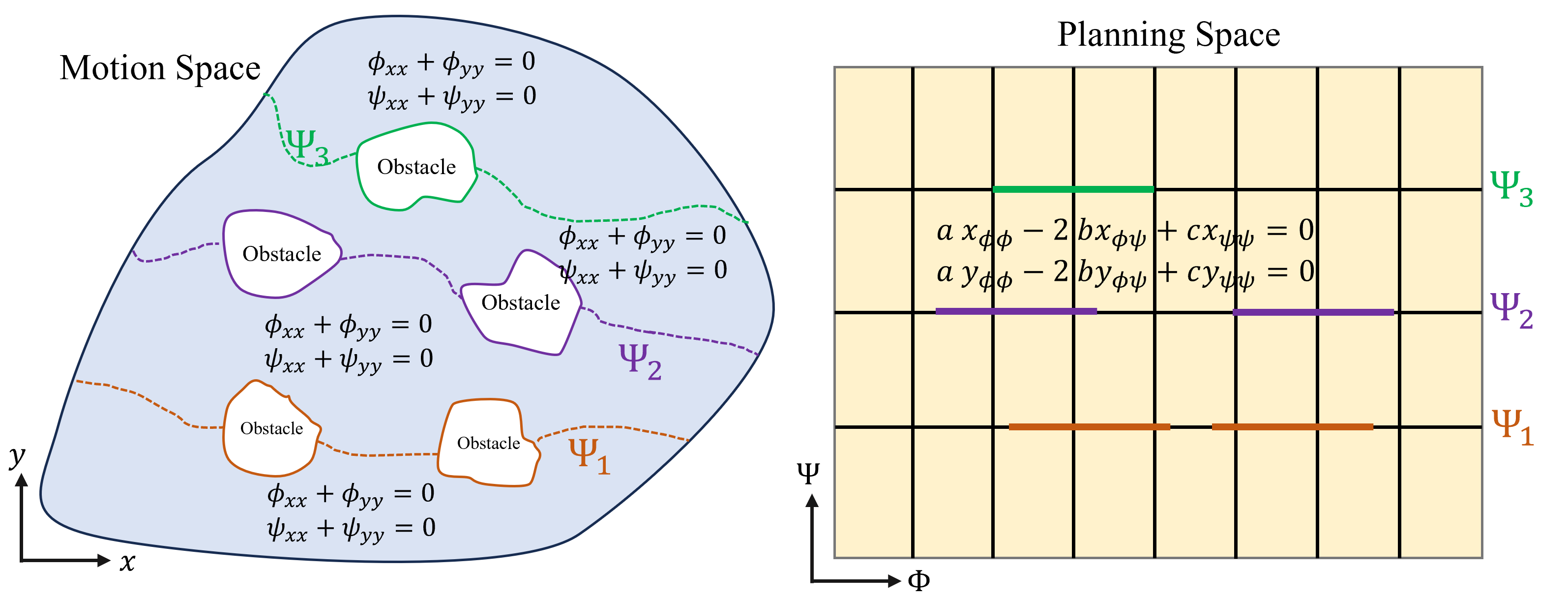
We propose a novel approach for safe and collision-less motion planning, wherein each obstacle is treated as a “rigid” body whose boundary is determined by two streamlines, having the same steam value and enclosing (or sandwiching) the obstacle. Inspired by the mesh generation techniques used for computational fluid dynamics applications, we will overcome the issue highlighted in Section I-A by (i) dividing the motion space into multiple navigable spaces, (ii) classifying obstacles into a finite number of groups, and (iii) sandwiching each obstacle group by two adjacent navigable channels (See Fig. 1). As a result, we can establish a non-singular transformation between and plane with forbidden crossing over finite number of horizontal line segments in the planning space. Compared to the available motion planning methods, our approach offers the following contributions:
-
•
We obtain the optimal path with a shorter length by A* searching over the planning space instead of motion space.
-
•
We consider obstacles as rigid-bodies with boundaries that cannot be trespassed since obstacles are excluded when we map the motion space to the planning space.
-
•
The optimal path minimizing travel distance between the initial location and target destination is obtained by searching over a uniform grid with geodesically varying distances and constrained transition.
We apply model predictive control (MPC) for the safety-verified trajectory tracking control where safety constraints are defined as linear inequalities.
This paper is organized as follows: Problem Statement is given in Section II. The motion planning approach is presented as Spatial and Temporal planning problems in Sections III and IV, respectively. Safety-verified MPC-based trajectory tracking is formulated in Section V. Simulation results are presented in Section VI and followed by concluding remarks in Section VII.
II Problem Statement
We consider robot motion planning in an obstacle-laden motion space and decompose it into spatial and temporal planning problems. Section III proposes to exclude obstacles by transforming the “motion” space into the “planning” space, and ensuring collision avoidance by robot motion planning in the planning space. The temporal planning is achieved through A* searching over a uniform grid distributed over the planning space as discussed in Section IV.
For the trajectory tracking control, without loss of generality, we consider quadcopter as the robot navigating in an obstacle-laden environment and the dynamics developed in Refs. [13, 14] to model its motion. Then, the trajectory tracking control is formulated as MPC in Section V.
Remark 1.
This paper assumes that the motion space is two dimensional where we use and to denote position components. For -D motion planning, we can decompose the motion space into parallel horizontal floors where and can be used to specify position in every floor.
III Spatial Planning
We use to denote the motion space, and decompose it into navigable subspace and obstacle subspace (). We apply the ideal fluid flow concept to establish a nonsingular mapping between navigable subspace , with position coordinates and , and the planning space, with position coordinates and , where we to refer to the planning space. Note that and are the potential and stream fields over the motion space, and maintain the following properties:
Property 1: Every obstacle in is wrapped by a -constant manifold which is a steamline in the motion space.
Property 2: Potential lines -constant and streamlines -constant are all perpendicular at any crossing point in .
Property 1 is achieved, when stream () values are constant along the outer boundary of every obstacle [11].
By achieving Property 2, both and , defined over the physical domain, satisfy the Laplace partial differential equation (PDE):
| (1a) | |||
| (1b) |
As mentioned in Section I-A, obtaining and is challenging by solving Laplace PDEs (1a) and (1b), when obstacles of random sizes and shapes are arbitrarily distributed over the motion space. We propose to define and as functions of independent variables and , and then use the chain rules to obtain derivatives of dependent variables and with respect to and . This establishes a mapping between the navigable space and the planning space, and converts the Laplace PDEs (1a) and (1b) to the following PDEs [15]:
| (2a) | |||
| (2b) |
where , , and .
We use finite difference approach to solve the elliptic PDEs (2a) and (2b). To this end, we first provide a solution for dividing into multiple obstacle-free navigable subspaces in Section III-A. We then specify boundary conditions to determine and over the planning space, by solving governing PDEs (2a) and (2b).
III-A Motion Space Decomposition and Obstacle Sandwiching
We consider a motion space consisting of obstacles, where each obstacle is a compact zone in , and obstacles are identified by set . We express as
| (3) |
where is a group of obstacles with the same values on their external boundaries. For example, obstacles shown in the motion space shown of Fig. 1 is categorized into three groups , , and , where obstacles of all wrap by two streamlines having the same value , for .
Given , the navigable zone is expressed as
| (4) |
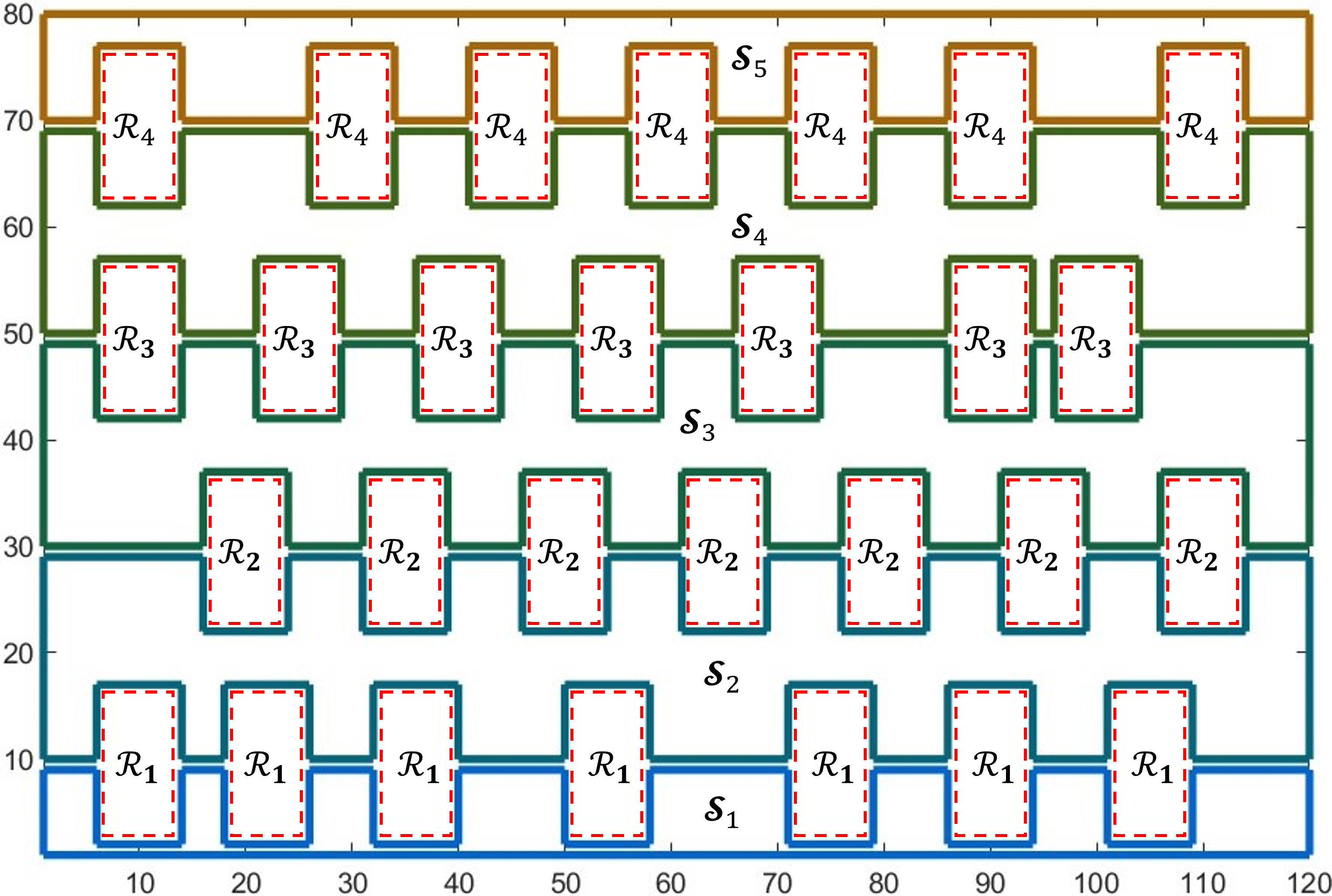
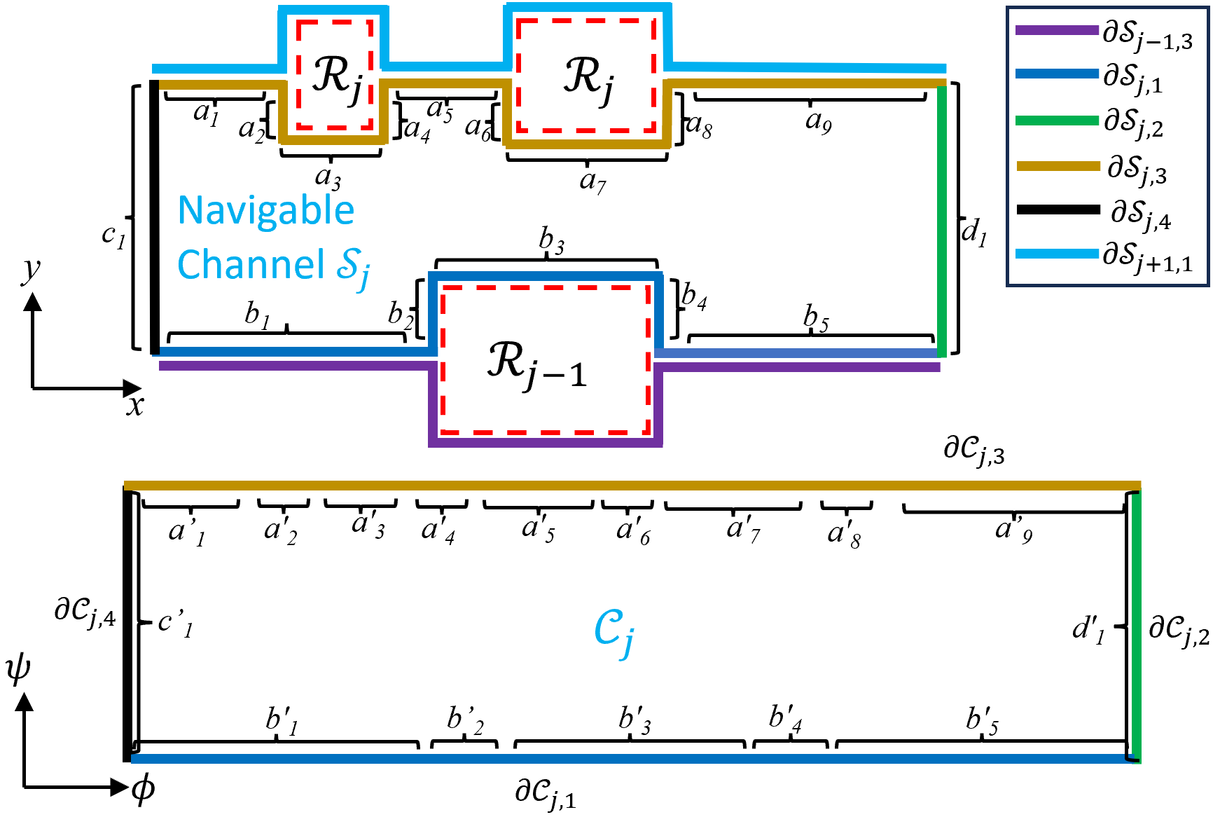
where is called the -th navigable channel. Note that all obstacle zones defined by are sandwiched by navigable channels and . For better clarification, we consider the rectangular motion space shown in Fig. 2 with obstacles categorized as through , is decomposed into five navigable channels (); and is sandwiched by navigable channels and for . We use , , , and to define the bottom, right, top, and left boundaries of , respectively (See Fig. 3).
III-B Planning Space Decomposition
The planning space is a rectangle defined by
| (5) |
where and , , , and are constant, , and . We divide into horizontal sub-rectangles, therefore,
| (6) |
where defines the -th sub-rectangle in planning space. We distribute a uniform grid over . Therefore, a total of of nodes are distributed over the planing space, where . We use , , , and to define the bottom, right, top, and left boundaries of , respectively. We note that the nodes scattered over coincide with the nodes distributed over .
III-C Boundary Conditions
To obtain boundary conditions of PDEs (2a) and (2b), the nodes on are uniformly mapped over , for and . Then, every node , positioned at has corresponding position . Therefore, and are known along the boundary , and we can solve PDEs (2a) and (2b) as a Dirichlet problem.
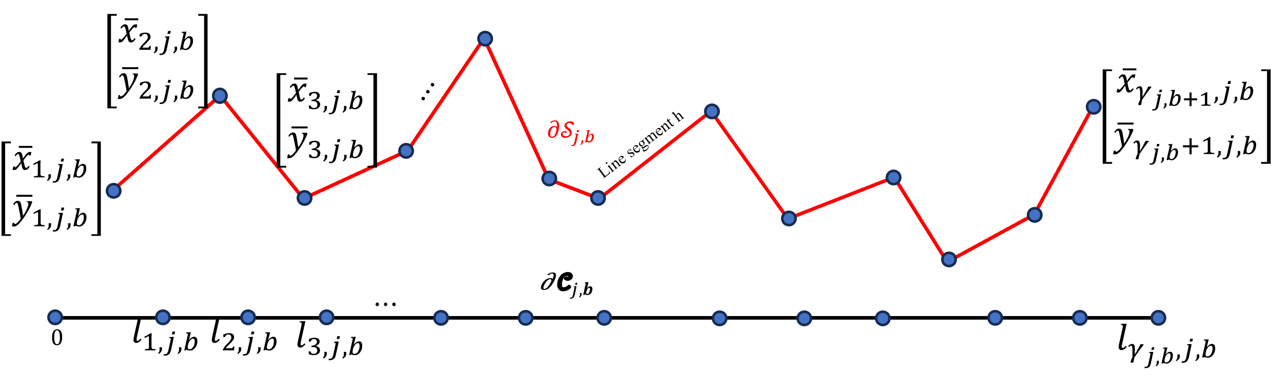
We use Algorithm 1 to uniformly distribute nodes along , when consists serially connected line segments connecting points given by finite sequence
We define
| (7a) | |||
| (7b) | |||
| (7c) |
as the length of the -th line segment on , the total length of boundary , and length increment, respectively, for , , and (See Fig. 4).
Definition 1.
Given boundary node , positioned at , and end points of the -line segments of positioned at and , we define vector operator We say the -th node is on the -th line segment connecting and , we define vector operator
| (8) |
for , , , and .
By using Definition 1, we can check whether boundary node is located on the -th line segment or not. If , then,
| (9a) | |||
| (9b) |
assign the and components of the -th node .
IV Temporal Planning
The objective of temporal planning is to obtain the desired trajectory between from the initial position to target destination in minimizing the travel distance. We define this problem as an A* search over the uniform grid distributed in . This search problem holds the following unique properties:
-
1.
Property 1: Operation, evaluation, and heuristic costs all depend on geodesic nodal distances.
-
2.
Property 2: There is no obstacle in the planning space, however, transitions over the uniform grid, distributed over the planning space , constrained over the nodes representing the obstacle boundaries in the actual motion space.
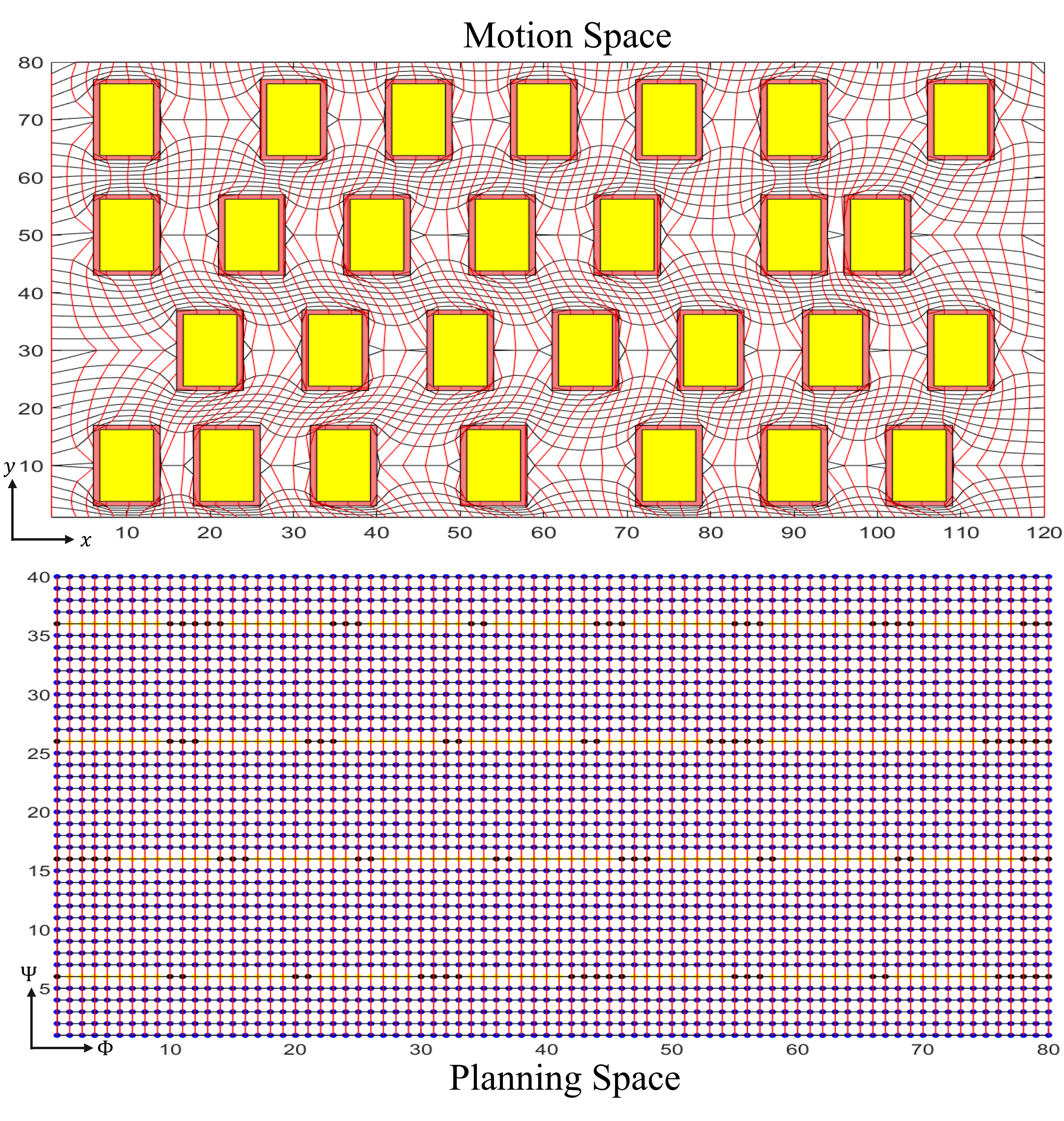
We note that Property 2 constrains paths designed over the planning space to not cross over the nodes representing obstacle boundaries in the planning space. For a better clarification, the bottom sub-figure in Fig. 5 is the planning space associated with the obstacle motion space shown in the top sub-figure, in Fig. 5, where the yellow dots represent the nodes distributed over the obstacle boundaries. It is not authorized that a robot trajectory, which is assigned by the A* searching in the planning space, crosses the yellow nodes in the planning space.
We showed that the implementation of an A* search in the planning space can generate a shorter path, compared to the existing A* search conducted over the motion space . This will be discussed in Section VI.
V Trajectory Tracking Control
Without loss of generality, this paper assumes that the robot is a quadcopter modeled by the dynamics presented in [13, 14]. By using the feedback liberalization approach (presented in [13, 14]), the quadcopter dynamics are converted to the following external and internal dynamics:
| (10a) | |||
| (10b) |
where denotes the discrete time; aggregates quadcopter’s position, velocity, acceleration, and jerk; aggregates yaw and time derivative of yaw; is the snap control; and is the control input of the internal dynamics. Also,
| (11a) | |||
| (11b) |
are time-invariant, where time increment is constant, is the identity matrix, and is the zero-entry matrix. We choose
| (12) |
and select constant gain matrix such that eigenvalues of the characteristic equation
| (13) |
are inside the unit disk centered at the origin. Therefore, asymptotically converges to , and therefore, the quadcopter motion is modeled by the external dynamics (10a).
V-A Safety Constraints
We suppose that the quadcopter moves horizontally at elevation and specify the desired trajectory by sequence
| (14) |
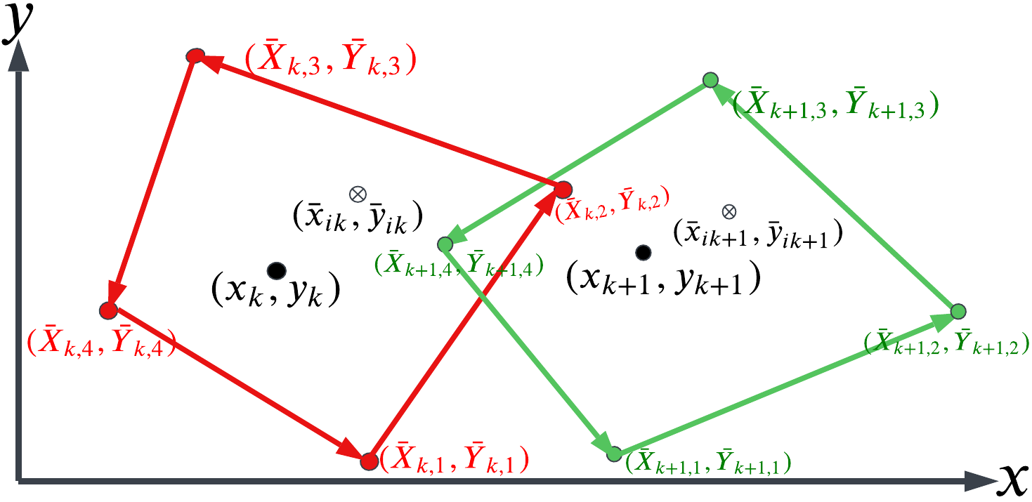
where aggregates and components of the quadcopter’s desired way-point obtained by the planning approach discussed in Section III-B, through A* searching in . We note that a nonsingular mapping exists between and . Desired position is enclosed by a neighboring quadrangle whose vertices are positioned at , , , and . Figure 6 shows the schematic of the neighboring quadrangle at two consecutive times and . To ensure collision avoidance, and components of quadcopter’s actual position, denoted by and , are constrained to be inside the neighboring quadrangle at every time . By defining and , this safety requirement is assured, if the following inequality condition is satisfied:
| (15) |
V-B MPC-Based Trajectory Tracking
We use the MPC method to determine the control input so that the is stably tracked while the safety constraints given by Eq. (16) are satisfied. To this end, we define
|
|
(18) |
as the MPC cost, where is a diagonal weight matrix, is the length of the prediction window, and denote quadcopter’s actual position components at time , and is a scaling factor.
Given dynamics (10a), we define vector and relate it to (the state vector at time ) and by
| (19) |
where and are obtained as follows:
| (20a) | |||
| (20b) |
We also use to aggregate the prediction of and components of the quadcopter’s actual position at time through , where and are related by
| (21) |
with . Furthermore, we use to aggregate the robot desired positions at time steps through .
The control objective is to minimize such that safety constraint equations, given by Eq. (16), is satisfied, where is enforced to be equal to at every discrete time . This problem can be formulated as a quadratic programming by
subject to
where
| (22) |
| (23) |
| (24) |
| (25) |
| (26) |
| (27) |
VI RESULTS
We consider quadcopter motion planning and control in the obstacle-laden motion space shown in Fig. 5. We use the spatial planning method presented in Section III to split the motion space into navigable space and obstacle zone , where: is decomposed into navigable channels through ; and sandwich all obstacles defined by , for , as illustrated in Fig. 2. We use the algorithmic approach presented in Section III-C to solve the governing PDE (2) using the Finite Difference method. We obtain the potential and steam lines that are shown by red and black curves in Fig. 5.
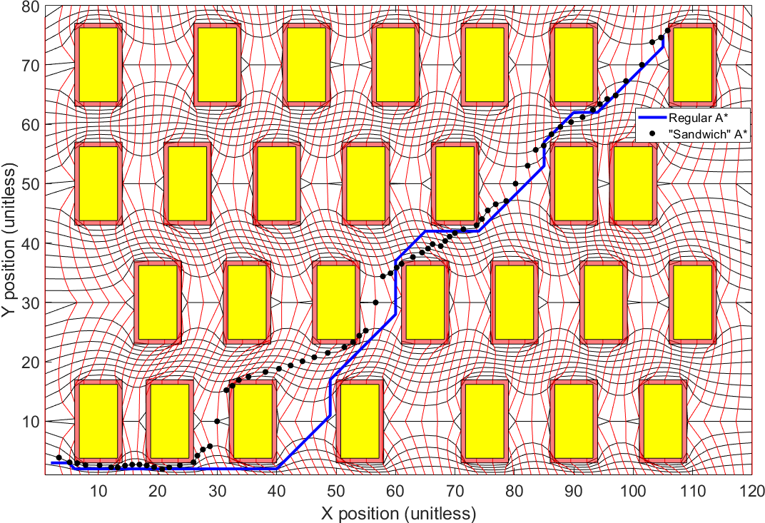
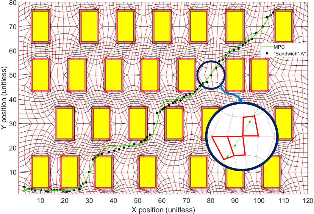
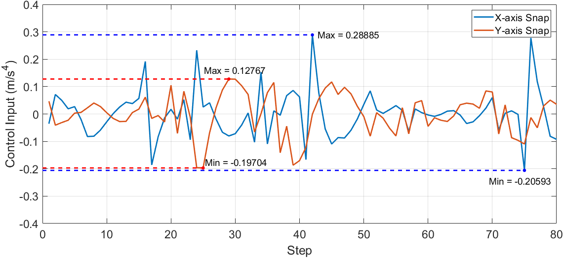
Given initial and final positions, we applied A* to obtain the quadcopter desired trajectory by searching over the planning space as detailed in Section IV. This desired trajectory is shown by black dots in Fig. 7. By applying regular A*, through searching over the motion space, we also obtained the blue path shown in Fig. 7 as the optimal path. Comparing the results, we observe of length reduction when the A* search is conducted over the planning space (See Table I). By adopting the quadcopter model presented in Section (II), we applied the MPC-based trajectory tracking control, presented in Section V-B, to stably and safely track the quadcopter’s desired trajectory where all safety requirements. The quadcopter’s actual path is shown by green 8. Figure 8 shows that the quadcopters’ actual positions are enclosed by the neighboring quadrangles. Figure 9 plots the and components of the snap control versus discrete time .
| Existing A* | Sandwich A* | |
|---|---|---|
| Length |
VII CONCLUSION
We developed a new approach for motion planning in constrained environments. We showed how we can exclude obstacles from the motion space by establishing a nonsingular mapping between the motion space and the planning space. We also obtained shorter paths between initial and target locations by applying search methods over the planning space instead of searching over the motion space. We also developed an MPC-based trajectory tracking control for a quadcopter navigating in an obstacle-laden environment, where we abstained and enforced safety requirements as linear constraints.
Acknowledgment
This work has been supported by the National Science Foundation under Award Nos. 2133690 and 1914581.
References
- [1] A. D. Ames, S. Coogan, M. Egerstedt, G. Notomista, K. Sreenath, and P. Tabuada, “Control barrier functions: Theory and applications,” in 2019 18th European Control Conference (ECC), 2019, pp. 3420–3431.
- [2] F. Ferraguti, C. T. Landi, A. Singletary, H.-C. Lin, A. Ames, C. Secchi, and M. Bonfè, “Safety and efficiency in robotics: The control barrier functions approach,” IEEE Robotics & Automation Magazine, vol. 29, no. 3, pp. 139–151, 2022.
- [3] J. Breeden and D. Panagou, “High relative degree control barrier functions under input constraints,” in 2021 60th IEEE Conference on Decision and Control (CDC). IEEE, 2021, pp. 6119–6124.
- [4] R. Cheng, G. Orosz, R. M. Murray, and J. W. Burdick, “End-to-end safe reinforcement learning through barrier functions for safety-critical continuous control tasks,” in Proceedings of the AAAI conference on artificial intelligence, vol. 33, no. 01, 2019, pp. 3387–3395.
- [5] J. Zeng, B. Zhang, and K. Sreenath, “Safety-critical model predictive control with discrete-time control barrier function,” in 2021 American Control Conference (ACC), 2021, pp. 3882–3889.
- [6] R. Grandia, F. Farshidian, R. Ranftl, and M. Hutter, “Feedback mpc for torque-controlled legged robots,” in 2019 IEEE/RSJ International Conference on Intelligent Robots and Systems (IROS), 2019, pp. 4730–4737.
- [7] Z. Marvi and B. Kiumarsi, “Safety planning using control barrier function: A model predictive control scheme,” in 2019 IEEE 2nd Connected and Automated Vehicles Symposium (CAVS). IEEE, 2019, pp. 1–5.
- [8] V. Varun, A. P. Vinod, and S. Kolathaya, “Motion planning with dynamic obstacles using convexified control barrier functions,” in 2021 Seventh Indian Control Conference (ICC). IEEE, 2021, pp. 81–86.
- [9] D. G. Crowdy, “Analytical solutions for uniform potential flow past multiple cylinders,” European Journal of Mechanics-B/Fluids, vol. 25, no. 4, pp. 459–470, 2006.
- [10] ——, “Uniform flow past a periodic array of cylinders,” European Journal of Mechanics-B/Fluids, vol. 56, pp. 120–129, 2016.
- [11] H. Rastgoftar and E. Atkins, “Physics-based freely scalable continuum deformation for uas traffic coordination,” IEEE Transactions on Control of Network Systems, vol. 7, no. 2, pp. 532–544, 2019.
- [12] A. E. Asslouj, E. Atkins, and H. Rastgoftar, “Can a laplace pde define air corridors through low-altitude airspace?” in 2023 International Conference on Unmanned Aircraft Systems (ICUAS), 2023, pp. 1–8.
- [13] H. Rastgoftar and I. V. Kolmanovsky, “Safe affine transformation-based guidance of a large-scale multiquadcopter system,” IEEE Transactions on Control of Network Systems, vol. 8, no. 2, pp. 640–653, 2021.
- [14] A. El Asslouj and H. Rastgoftar, “Quadcopter tracking using euler-angle-free flatness-based control,” in 2023 European Control Conference (ECC). IEEE, 2023, pp. 1–6.
- [15] K. Hoffmann and S. Chiang, Computational Fluid Dynamics for Engineers, ser. Computational Fluid Dynamics for Engineers. Engineering Education System, 1993, no. v. 1. [Online]. Available: https://books.google.com/books?id=k_xQAAAAMAAJ