Vidaptive: Efficient and Responsive Rate Control for Real-Time Video
on Variable Networks

Abstract

Real-time video streaming relies on rate control mechanisms to adapt video bitrate to network capacity while maintaining high utilization and low delay. However, the current video rate controllers, such as Google Congestion Control (GCC) in WebRTC, are very slow to respond to network changes, leading to link under-utilization and latency spikes. While recent delay-based congestion control algorithms promise high efficiency and rapid adaptation to variable conditions, low-latency video applications have been unable to adopt these schemes due to the intertwined relationship between video encoders and rate control in current systems.

This paper introduces Vidaptive, a new rate control mechanism designed for low-latency video applications. Vidaptive decouples packet transmission decisions from encoder output, injecting “dummy” padding traffic as needed to treat video streams akin to backlogged flows controlled by a delay-based congestion controller. Vidaptive then adapts the frame rate, resolution, and target bitrate of the encoder to align the video bitrate with the congestion controller’s sending rate. Our evaluations atop WebRTC show that, across a set of cellular traces, Vidaptive achieves $\sim$2$\times$ higher video bitrate and 1.6 dB higher PSNR, and it reduces $95^{\text{th}}$-percentile frame latency by $2.7$s with a slight increase in median frame latency.

1 Introduction

Real-time video streaming has become an integral part of modern communication systems, enabling a wide range of applications from video conferencing to cloud gaming, live video, and teleoperation. A critical component of these systems is the rate control mechanism, which adapts the video bitrate to the available network capacity. State-of-the-art rate controllers, however, such as the Google Congestion Control (GCC) [1] algorithm used in WebRTC [2] have significant shortcomings. Specifically, GCC is slow to adapt to changes in network conditions, leading to both link under-utilization and latency spikes.

In recent years, numerous congestion control algorithms (CCA) have been proposed that achieve high utilization, low delay, and fast convergence [3, 4, 5, 6]. These algorithms are highly responsive to network variations, adapting within a few round-trip times (RTTs) while maintaining high utilization and low delay. In contrast, GCC and similar video rate control algorithms lag considerably. When network bandwidth opens up, GCC can take an order of magnitude longer than state-of-the-art congestion controllers to increase the video bitrate. This conservative approach can significantly hurt GCC’s utilization and the video quality in variable networks. In our experiments using cellular network traces, GCC under-utilizes the network by 2-3$\times$ compared to Copa [3].

This sluggishness is not merely a limitation of GCC but a symptom of a broader issue: the inherent coupling between video encoders and rate control algorithms [7]. Current systems use an encoder-driven rate controller that adapts the video bitrate by controlling the encoder’s target bitrate. In these systems, the instantaneous data transmission rate is dictated by the size of the video frames produced by the encoder. However, most video encoders are not designed to adjust to rapid fluctuations in network conditions. It generally takes several frames to adapt frame sizes to new target bitrates [7]. Moreover, the frame sizes are variable and only meet the target bitrate on average in a best-effort manner. To maintain low latency despite the vagaries of the encoder output, GCC sets the target bitrate conservatively and increases it slowly. Nevertheless, during times of significant congestion (e.g., due to link outages), the encoder cannot immediately adapt to capacity drops, and GCC experiences significant latency spikes.

Recently, Salsify [7] addressed this challenge by modifying the encoder to be more adaptive to network variations. Such approaches, however, are challenging to deploy in practice. Changing the encoder usually requires changes to both the sender and receiver sides of the application. With the prevalence of hardware codecs across billions of devices, such drastic changes have become virtually infeasible.

We present Vidaptive, a new rate control mechanism for low-latency video applications that significantly improves efficiency and responsiveness to network variability without modifying the encoder. Vidaptive’s design is based on two key concepts.

The first is to decouple instantaneous packet transmission decisions from the encoder’s output. Specifically, Vidaptive treats video streams as if they were backlogged flows for the purpose of rate control. It uses an existing delay-based CCA like Copa. If the encoder produces more packets than the CCA is willing to send, it buffers them at the sender. On the other hand, Vidaptive sends “dummy packets” to fill the gap if the encoder does not produce enough packets to sustain the CCA’s rate. This approach ensures that “on the wire”, Vidaptive behaves identically to its adopted CCA running with a backlogged flow. The CCA’s feedback loop can operate without disruption and track available bandwidth quickly.

Next, Vidaptive matches the video bitrate to the CCA’s sending rate using mechanisms that adapt the frame rate, the encoder’s target bitrate, and the video resolution. To keep frame latency within acceptable bounds when the encoder overshoots the CCA’s rate, Vidaptive skips a frame if the delay at the sender exceeds a threshold (effectively reducing the frame rate to handle sudden latency spikes). Further, Vidaptive uses a novel online optimization algorithm to determine the encoder’s target bitrate based on the CCA’s sending rate and recent frame delay measurements. The optimization procedure provides a principled approach to navigate the tradeoff between video bitrate and frame rate, and importantly, it adapts automatically to the variability in the encoder’s output and the network rate.

We implement Vidaptive atop WebRTC and test it using sixteen cellular network traces with significant variability on an emulated network link [8]. Compared to GCC, our key findings are:

1. Across all traces, Vidaptive improves link utilization by $\sim$2.5$\times$ and video bitrate by $\sim$2$\times$ on average across all traces, resulting in 1.6dB improvement in Peak-Signal-to-Noise-Ratio (PSNR) on average.

2. Across all frames in all traces, Vidaptive improves average PSNR by 1.9 dB and P95 PSNR by 2.2 dB.

3. Across all frames in all traces, Vidaptive increases median latency by 47 ms (148 ms $\rightarrow$ 195 ms), but it reduces $95^{th}$ percentile frame latency by 2687 ms (4120 ms $\rightarrow$ 1433 ms). On a per-trace basis, Vidaptive improves P95 frame latency by $\sim$ 2.7 seconds on average but is 45-384 ms worse on some traces.

4. Vidaptive reduces frame rate by $\sim$ 10% on average per trace.

2 Motivation and Key Ideas

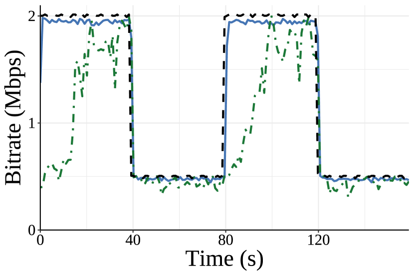
(a) Link Utilization

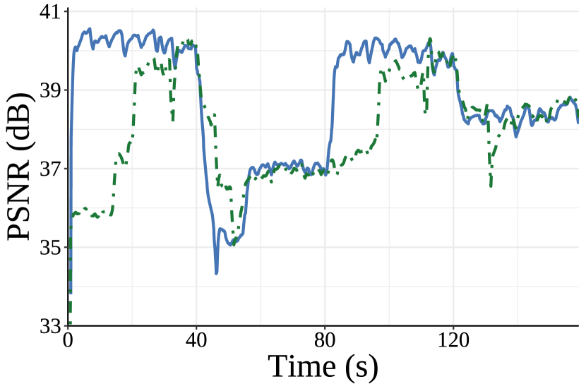
(b) Frame Quality

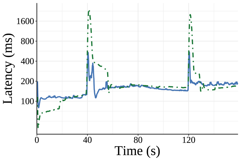
(c) Frame Latency

Figure 1: Utilization, frame quality, and latencies of Copa on a backlogged flow, GCC on a video flow, and Copa + Vidaptive on a video flow. GCC is very slow to match the available capacity and under-utilizes the link in the steady state. Copa + Vidaptive responds much faster to link variations and is similar to Copa’s performance on a backlogged flow.

2.1 The Problem

Status Quo for Video Rate Control. To understand how rate control for real-time video works today, we run Google Congestion Control (GCC) [1], the rate control mechanism inside WebRTC, on an emulated link that alternates between $2\text{\,}\mathrm{M}\mathrm{b}\mathrm{p}\mathrm{s}$ and $500\text{\,}\mathrm{K}\mathrm{b}\mathrm{p}\mathrm{s}$ every 40 seconds. The minimum network round-trip time (RTT) is $50\text{\,}\mathrm{m}\mathrm{s}$, and the buffer size at the bottleneck is large enough that there are no packet drops. In Fig. 1(a), GCC is sluggish to increase its rate when the stream begins and when the link capacity rises back to $2\text{\,}\mathrm{M}\mathrm{b}\mathrm{p}\mathrm{s}$ at $t=80$s. Specifically, GCC takes 18 seconds to go from $500\text{\,}\mathrm{K}\mathrm{b}\mathrm{p}\mathrm{s}$ to $2\text{\,}\mathrm{M}\mathrm{b}\mathrm{p}\mathrm{s}$, resulting in lower visual quality during that time (Fig. 1(b)). GCC’s conservative nature also results in link under-utilization (85%) in the steady state. GCC is slow to react to capacity drops: in Fig. 1(c), when the link rate drops to $500\text{\,}\mathrm{K}\mathrm{b}\mathrm{p}\mathrm{s}$ at $t=40$s, GCC’s frame latency spikes to over a second and settles only after 12 seconds. This issue is because GCC continues to send at a higher rate even after the drop, causing queue buildup, added delay, and frame loss.

Contrast this behavior with traditional congestion control algorithms [3, 9, 10, 4] operating on backlogged flows: they respond to such network events much faster, typically over few RTTs. For instance, the “Backlogged Copa” lines in Fig. 1(a) and Fig. 1(c) show that Copa [3], running on a backlogged flow on the same time-varying link is much more responsive to the network conditions. This wide disparity between GCC on real-time video traffic and Copa on backlogged traffic begs the question: Why does the state-of-the-art video rate control lag so far behind the state-of-the-art congestion control?

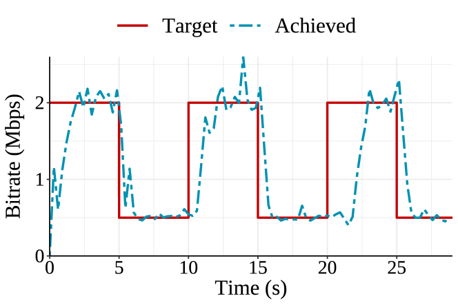
Figure 2: Video encoder’s response to a time-varying “Target” input bitrate. “Achieved” reflects the encoder’s output rate. The encoder is slow to increase its output rate and exhibits a lot of variation around the average output rate in the steady state.

Encoder-driven Rate Control Loop. GCC has been carefully designed to work within the tight latency bounds of interactive video applications. Its rate control responds to increases or decreases in delay gradients over RTT timescales. It is also conservative in its link utilization to not overwhelm the network and cause delays or packet loss.

However, the real limiting factor is that, in current video congestion controllers like GCC, the instantaneous rate at which data is transmitted on the wire is dictated by the size of the video frames produced by the encoder. GCC controls the video bitrate by adapting the encoder’s target rate, but the encoded frame sizes can be highly variable. The encoder achieves its target bitrate only on average—usually throughout several frames [7]. Moreover, the encoder’s bitrate cannot immediately adapt to changes in the target bitrate. We illustrate this behavior in Fig. 2 where we supply the VP8 encoder with a target bitrate that switches between $2\text{\,}\mathrm{M}\mathrm{b}\mathrm{p}\mathrm{s}$ and $500\text{\,}\mathrm{K}\mathrm{b}\mathrm{p}\mathrm{s}$ every 5s and observe its achieved bitrate. Every time the bitrate goes up from $500\text{\,}\mathrm{K}\mathrm{b}\mathrm{p}\mathrm{s}$ to $2\text{\,}\mathrm{M}\mathrm{b}\mathrm{p}\mathrm{s}$, the encoder takes nearly 2 seconds to catch up. On the way down from $2\text{\,}\mathrm{M}\mathrm{b}\mathrm{p}\mathrm{s}$ to $500\text{\,}\mathrm{K}\mathrm{b}\mathrm{p}\mathrm{s}$, it takes about a second to lower the bitrate.

The reason for this lag is that the size of an encoded frame is dependent on several factors, including quantization parameters, the encoder’s internal state, and the motion, and is only known accurately after encoding. The encoder tries to rectify its over- and under-shootings by adjusting the quality of subsequent frames. Even once the encoder matches the target bitrate, it exhibits considerable variance around the average on a per-frame basis. Salsify [7] deals with this unpredictability by encoding multiple versions of the same frame and picking the best match after the fact. However, putting aside the extra computational cost, this approach requires radical changes to the codec—at both the sender and the receiver—which hinders its real-world deployability.

The unpredictable nature of the encoder leads to two main issues: (1) Since the encoder cannot match the target bitrate on per-frame timescales, GCC cannot immediately reduce the bitrate if the capacity suddenly drops. Instead, GCC has to be conservative and leave abundant bitrate headroom at all times (including in the steady state) so that it reduces the risk of congestion during fluctuations. Despite this, GCC still experiences occasional latency spikes (Fig. 1(c)). (2) GCC is very slow to grab available bandwidth. Whenever GCC increases its target bitrate, the encoder matches it over a few seconds, meaning it also takes several seconds for GCC to get feedback at the higher rate and increase its target bitrate again. This cycle ends up taking 15–20 seconds end-to-end (Fig. 1(a)).

What about Probing Mechanisms? A natural question at this point is if probing mechanisms, specifically those already supported within GCC [11], improve GCC’s convergence in such scenarios. While periodic bandwidth probing has proved effective for some CCAs [4], the GCC mechanism is relatively ad-hoc. It fires a periodic timer and sends some bounded extra padding traffic (the frequency can vary but is often in the range of seconds (e.g., every $5\text{\,}\mathrm{s}\mathrm{e}\mathrm{c}\mathrm{o}\mathrm{n}\mathrm{d}\mathrm{s}$)). Such an infrequent timer does not help on the finer RTT-level timescales required for precise rate control. A five-second timer is, in practice, very similar to a sluggish encoder that responds to the target bitrate over a few seconds. Fig. 3 shows how GCC with probing enabled reacts on a lossless periodic link with an RTT of $50\text{\,}\mathrm{m}\mathrm{s}$ that alternates between $2\text{\,}\mathrm{M}\mathrm{b}\mathrm{p}\mathrm{s}$ and $500\text{\,}\mathrm{K}\mathrm{b}\mathrm{p}\mathrm{s}$ every $40\text{\,}\mathrm{s}\mathrm{e}\mathrm{c}\mathrm{o}\mathrm{n}\mathrm{d}\mathrm{s}$. The padding traffic is only sent when GCC reduces the video bitrate significantly (t=40s) but does not help at all with bandwidth discovery (t=80s) when the link opens back up.

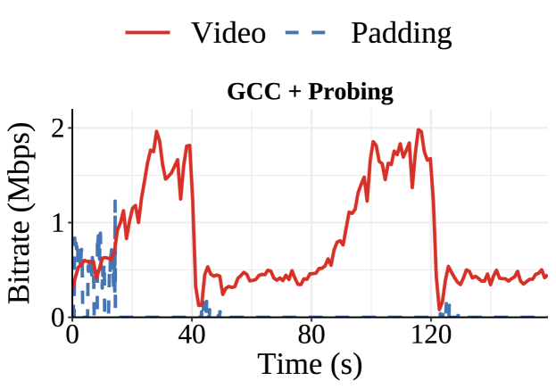
Figure 3: Ad-hoc Probing Behavior in WebRTC on a periodic link that alternates between $2\text{\,}\mathrm{M}\mathrm{b}\mathrm{p}\mathrm{s}$ and $500\text{\,}\mathrm{K}\mathrm{b}\mathrm{p}\mathrm{s}$ every 40s. Padding traffic is used when GCC’s estimate severely drops (t=40s) but not used when needed during the capacity increase (t=80s).

2.2 Our Solution

Decoupling the Encoder from the Rate on the Wire. As illustrated in Fig. 1(a), a backlogged flow using a state-of-the-art CCA like Copa can adapt to time-varying network capacity on RTT timescales while also controlling network queueing delay. A key reason is that such CCAs have fine-grained control over when to send each packet, e.g., driven via the “ACK clock” [12]. Vidaptive makes video streams appear like a backlogged flow to the congestion controller. This allows Vidaptive to leverage existing CCAs optimized for high throughput, low delay, and fast convergence. In Fig. 1, Vidaptive using Copa for congestion control achieves nearly identical throughput and latency as a backlogged Copa flow. Vidaptive quickly increases its bitrate when bandwidth opens up, leading to higher image quality than GCC following each such event (Fig. 1(b)).

Vidaptive sends packets on the wire as dictated by the congestion controller. Specifically, when the encoder overshoots the available capacity, Vidaptive queues excess video packets in a buffer and only sends them out when congestion control allows (e.g., according to the congestion window and in-flight packets for window-based CCAs). Conversely, when the encoder undershoots the available capacity, Vidaptive sends “dummy packets” to match the rate requested by the congestion control by padding the encoder output with additional traffic. This allows the CCA to operate without disruption (as in a backlogged flow) despite the encoder’s varying frame sizes.

By decoupling the congestion control’s decisions from the encoder output, Vidaptive can accurately track time-varying bottleneck rates. However, it is still important to match the actual video bitrate produced by the encoder to the congestion controller’s sending rate. In particular, although buffering packets and sending dummy traffic can handle brief variations in the encoder output bitrate, the quality of experience will suffer if the encoder’s output is persistently higher or lower than the congestion control’s rate. In the former case, end-to-end frame latency would grow uncontrollably, and in the latter scenario, dummy packets would waste significant bandwidth.

Vidaptive includes two mechanisms that control the frame rate and encoder’s target bitrate to match the video bitrate to the congestion controller’s sending rate while meeting a delay constraint. First, it uses simple safeguards to ensure that end-to-end frame latency is not significantly affected by delay at the sender. If the delay at the sender exceeds a threshold, Vidaptive skips a frame. During severe latency spikes (e.g., caused by a network outage), Vidaptive drops buffered packets and resets the encoder using a keyframe.

Second, Vidaptive selects the encoder’s target bitrate by solving an online optimization that decides how much headroom to leave between the target bitrate and the CCA’s sending rate (CC-Rate). Increasing the target bitrate to near the CC-Rate (lowering headroom) provides a higher video bitrate (and better quality). However, it risks latency increases due to the variability of the encoder’s output frame sizes and future sending rate fluctuations. If these latency increases exceed the video’s delay tolerance, Vidaptive has no choice but to reduce the frame rate. Thus, the choice of the target bitrate (headroom) is effectively about navigating a tradeoff between video bitrate and frame rate. This tradeoff depends on the inherent variability of the system. If the encoder’s output and the bottleneck link rate (and hence CC-Rate) are stable and have low variance, then a small headroom can suffice to ensure low, consistent frame latency and, therefore, a high frame rate. However, the headroom must increase with more variability. Vidaptive’s online optimization uses recent frame delay measurements to adapt to such variability automatically.

3 Vidaptive Design

3.1 Overview

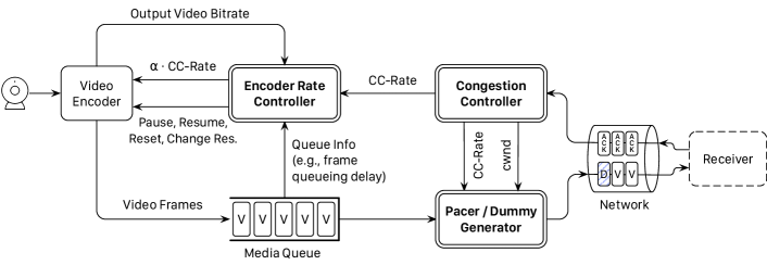
Figure 4: Vidaptive Design. Vidaptive uses a window-based Congestion Controller, Pacer, and a new Dummy Generator to decouple the rate at which traffic is sent on the wire from the encoder. The Encoder Rate Controller monitors frame delays to trigger latency safeguards and picks a new target bitrate and resolution based on the discrepancy between the CC-Rate and the video encoder’s current bitrate.

Our goal is to design a system for real-time video applications that responds quickly to any changes in network conditions, and maintains high utilization of available capacity without altering the encoder. Vidaptive achieves this by decoupling the behavior of the transport layer from the unreliable video encoder, and by closely matching the encoder bitrate to the CCA’s sending rate (CC-Rate).

Fig. 4 shows Vidaptive’s overall design. The video encoder encodes frames and sends them to an application-level media queue before sending the packets out into the network. At the transport layer, we add a modified window-based “Congestion Controller”, a “Pacer” and a new “Dummy Generator” to decouple the rate at which traffic is sent on the wire from the encoder, as described in §3.2. We introduce a new “Encoder Rate Controller” that monitors the delay frames are experiencing to trigger the latency safeguards described in §3.3. The rate controller also uses the discrepancy between the CC-Rate and the video encoder’s current bitrate, along with frame delays to adapt the target bitrate and resolution to efficiently trade off frame rate and frame quality (§3.4).

3.2 Transport Layer

Congestion Controller. To build a more responsive transport for real-time video, we start with a congestion controller that is more responsive to the network. A window-based algorithm keeps the amount of video packets in check without allowing them to grow uncontrollably and cause high latency, packet loss, and glitches. Specifically, the congestion window (cwnd) in Vidaptive tracks the maximum number of in-flight bytes between the sender and the receiver. cwnd increases when the queueing delay is lower than what the CCA hopes to impose and decreases otherwise. The sender only sends out new packets when the amount in-flight is less than cwnd. Using delay as the congestion signal prioritizes the end-to-end frame latency and adjusts the window such that most frames are delivered in real time. Vidaptive can be used with any delay-controlling congestion control algorithm. We evaluate Vidaptive with two recently proposed such algorithms, Copa [3] and RoCC [9].

We compute the system’s sending rate (CC-Rate) as the cwnd divided by smoothed RTT and use it to configure the Pacer and the encoder target bitrate (§3.4).

Pacer. The Pacer receives cwnd and the CC-Rate from the congestion controller and paces out the video packets at CC-Rate. Since the encoder exhibits variance and its output bitrate may instantaneously overshoot the available capacity (§2), the pacer is responsible for avoiding a sudden burst of packets. In Vidaptive, the pacing rate and the congestion window together determine when to send the next packet.

Dummy Packets. While the window-based CCA ensures ACK-clocked behavior, and the pacer prevents sudden bursts of video packets, neither ensures fast feedback between video frame boundaries. The lack of feedback prevents us from quickly growing our window when bandwidth opens up (§2). To emulate the behavior of a backlogged flow, we place “dummy packets” into the pacer’s queue if the CCA is ready to send a packet but has no available video packets. Note that the dummy packets never stay in the pacer queue as they are only generated when the CCA wants to send a packet, but the pacer queue is empty.

To avoid network delay spikes caused by spurious dummy packets when the link rate suddenly drops, we do not send any dummy packets within a few milliseconds ($5\text{\,}\mathrm{m}\mathrm{s}$ in our implementation) of reading frames from the camera. The intuition behind this mechanism is that if the network is soon to deteriorate, the dummy packets sent a few milliseconds prior to a frame will induce a higher queuing delay in the network and thus increase the frame latency. On the other hand, if the network rate opens up, not sending packets for a few milliseconds will not slow down the congestion controller’s convergence by much.

Lastly, we stop sending dummy packets if the video has reached a maximum bitrate ($12\text{\,}\mathrm{M}\mathrm{b}\mathrm{p}\mathrm{s}$ in our experiments). Since the video bitrate cannot increase further, sending extra traffic to discover more available bandwidth is not useful.

3.3 Safeguarding against Latency Spikes

Transport design for any real-time video system must ensure low-latency frame delivery. As a result, we place two safeguards within Vidaptive to avoid transmitting frames that are unlikely to be successfully received on time. These safeguards essentially reduce the frame rate during highly congested periods to mitigate latency spikes; we discuss our principled strategy for trading off frame rate with quality in §3.4.

Encoder Pause. Vidaptive monitors the time packets spend in the pacer queue before they are sent out. If the time spent by the oldest packet exceeds a pacer queue pause threshold ($\tau$), we pause encoding and buffer the latest un-encoded frame. If the CC-Rate increases and the pacer queue is drained, we resume encoding and send video packets from the latest buffered frame if it is within $\sim$ $17\text{\,}\mathrm{m}\mathrm{s}$ ($33\text{\,}\mathrm{m}\mathrm{s}$/2) of that frame being read. Otherwise, we skip this frame altogether and encode the next frame since we are closer in time to reading the next frame. We set $\tau$ = $33\text{\,}\mathrm{m}\mathrm{s}$ by default in our implementation, thereby pausing encoding if packets from the previous frame are yet to be sent out. The intuition here is that there is no point in encoding a frame that would have to sit in the Pacer queue, waiting for a previous frame to finish transmission. Instead, we always encode and transmit fresh frames when they have a high chance of reaching the receiver with acceptable latency.

Encoder Reset. If video packets have been stuck in the pacer for extended periods ($>$ 1s), the network is likely experiencing an outage or extreme congestion. Packets already sent out will likely be lost, making their corresponding frames not decodable. Sending more video packets dependent on those un-decodable frames is wasteful and makes application-level recovery harder. Furthermore, packets from these frames have already incurred a huge latency in the pacer queue, and sending them out would mean very high end-to-end frame latency. Instead, we drain the pacer entirely and reset the encoder by forcing it to send a keyframe. Since video packets received after the congestion event belong to a keyframe, the receiver’s decoder has no errors when decoding them. This reset, similar to pausing, has the impact of controlling worst-case frame latency. It also allows Vidaptive to choose very conservative target bitrates and resolutions (§3.4) in the aftermath of a congestion event that ensures that video packets get through to the receiver and give us fast feedback to help reset the system.

3.4 Trading off Frame Rate and Quality

Vidaptive skips encoding some frames to reduce latency as described in §3.3. Since this reduces the frame rate and affects the smoothness of the video, Vidaptive is set up to reduce the frame bitrate proactively and, consequently, the frame quality in favor of letting more frames get through.

We formalize the tradeoff between frame rate and frame quality as a decision problem that picks a target bitrate for the encoder based on how much we prioritize achieving a high frame rate over high video quality. Specifically, we pick $\alpha$, the fraction of the CC-Rate to supply as the target bitrate to the encoder. When the frame rate is low, we choose a smaller $\alpha$ to create smaller frames but let more of them get through. When the frame rate is high, we choose a higher $\alpha$ to obtain higher quality frames while sacrificing a little on the achieved frame rate. To affect significant and sudden changes in the video bitrate based on network conditions, we update the resolution in addition to setting the target bitrate.

Preliminaries. Vidaptive encodes each frame if the frame queueing delay (delay through the pacer queue) for the oldest unsent frame is not more than the pacer queue pause threshold $\tau$. We define Vidaptive’s frame rate score $\mathcal{F}$ to capture how many frames it successfully delivers over a time interval $T$. If there are $N$ frames over a time interval $T$ that experience delays through the pacer queue denoted by $d_{i}$ for $i\in\{1,2,..,N\}$, we define $\mathcal{F}$ as the ratio of the number of frames successfully sent (those whose queuing delays do not exceed $\tau$) to $N$, the total number of frames. In other words,

$$\mathcal{F}=\frac{\sum_{i=1}^{N}\mathbb{1}[d_{i}\leq\tau]}{N},$$ (1)

where $\mathbb{1}[d_{i}\leq\tau]=1$ if $d_{i}\leq\tau$ and 0 otherwise. At higher $\mathcal{F}$, most frames have $d_{i}\leq\tau$ and do not pause the encoder which results in a higher frame rate. $T=$1s by default in our implementation.

If the camera’s frame rate is $f_{max}$ (typically 30 FPS), the gap between frames is $\Delta=\frac{1}{f_{max}}$ (typically $33\text{\,}\mathrm{m}\mathrm{s}$). For maximum efficiency, the frame queueing delay should be close to $\Delta$, such that the last packet of a frame is transmitted just as the next frame is encoded. Thus, to measure Vidaptive’s efficiency and its impact on frame quality, we define its bitrate score $\mathcal{B}$ as,

$$\begin{split}\mathcal{B}=\min\Big{(}\frac{\sum_{i=1}^{N}d_{i}}{N\Delta},1\Big{)}\end{split}$$ (2)

Note that $\frac{\sum_{i=1}^{N}d_{i}}{N}$ is the average frame queueing delay over the $N$ samples in the last time interval $T$, and its ratio relative to $\Delta$ can be viewed as a proxy for utilization. For example, if $\mathcal{B}=0.2$, the system is sending 20% of the video traffic it can send to the link without causing additional delays.

Choosing a Target Bitrate. The frame queueing delay is a function of the estimation of the link rate, CC-Rate, and frame sizes. As a result, it is impacted by fluctuations in both the encoder’s output and in the CC-Rate. These fluctuations are out of our control and can be viewed as a form of exogenous “noise” impacting frame delays. However, we can influence the expected frame sizes by controlling the encoder’s target bitrate. The crux of our method is to pick the target bitrate in a way that maximizes a weighted linear combination of $\mathcal{F}$ and $\mathcal{B}$ based on recent per-frame queueing delay measurements. Assume a target bitrate $\alpha\cdot\text{{\tt CC-Rate}}$ is given to the encoder where $0<\alpha<1$. Increasing $\alpha$ increases each frame’s size and its $d_{i}$ (frame size divided by CC-Rate). Since $d_{i}$ depends on $\alpha$, we rename it $d_{i}(\alpha)$. Increasing $d_{i}(\alpha)$ increases $\mathcal{B}$ but reduces $\mathcal{F}$, i.e. $\alpha$ induces a tradeoff between the frame rate and the frame quality. Our goal is to find $\alpha^{*}$ such that:

$$\text{maximize}\quad\frac{\lambda}{1-\lambda}\mathcal{F}+\mathcal{B}$$ (3)

$$\textrm{s.t.}\quad 0<\alpha<1$$

where $\lambda\in(0,1)$ is a parameter that reflects how much the application favors higher frame rate over better frame quality. When $\lambda\sim 1$, the application favors a high frame rate; when $\lambda\sim 0$, the application favors larger frames and higher quality.

Solving the Optimization. To choose $\alpha$, one would ideally want to solve the above optimization problem over future frames. However, it is hard to model $d_{i}(\alpha)$ for future frames since these can depend on future video content (e.g., the extent of motion) and how CC-Rate changes in the future. Instead, we use hindsight optimization [15] to solve for the best $\alpha$ we could have picked in hindsight for recent past frames. Estimating the effect $\alpha$ would have had on the delays of previous frames is simple. Assume we have frame queueing delay measurements $d_{i}$ for $i\in\{1,2,..,N\}$ over a time interval $T$, and we encoded these frames with a target bitrate $\alpha_{i}\cdot\text{{\tt CC-Rate}}$. Had all these frames been encoded by $\alpha$ instead, the counterfactual frame queueing delay would have been $\tilde{d_{i}}(\alpha)=d_{i}\frac{\alpha}{\alpha_{i}}$. This estimate assumes that frame size is proportional to the target bitrate (and hence proportional to $\alpha$), and that changing the target bitrate would not have changed CC-Rate. Using these counterfactual delay estimates, we can now solve the optimization problem in Eq. (3).

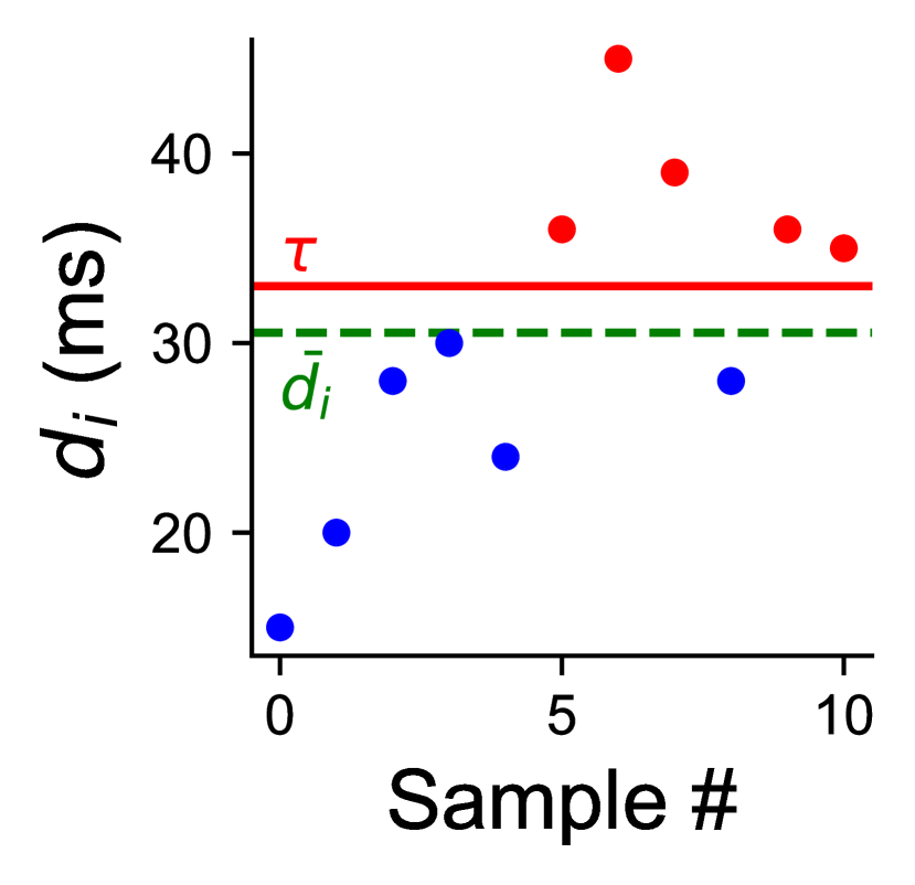
(a) Frame queueing delay samples

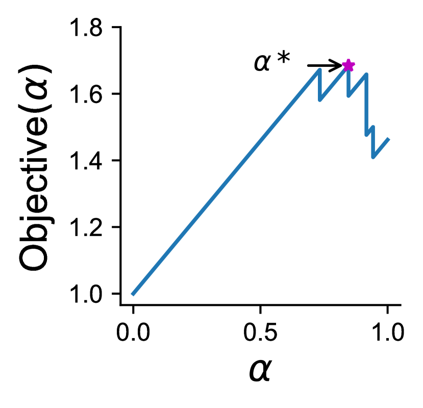
(b) Optimization Objective

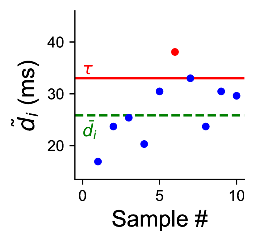
(c) Counterfactual optimization

Figure 5: Counterfactual optimization flow. Given a set of frame queueing delay samples (left), whose average is shown in green and outliers higher than $\tau$ are shown in red, we evaluate $\text{Objective}(\alpha)$ for discrete $\alpha$ and find $\alpha^{*}$ that maximizes it (middle). We update the counterfactual values of frame queueing delay with $\alpha^{*}$ to have fewer outliers above $\tau$ but a lower average (right).

Fig. 5 shows an example of this counterfactual optimization problem. Fig. 5(a) shows frame queueing delay samples and their average (green line). The samples that are less than $\tau$ are colored in blue, and those larger than $\tau$ (which would cause a frame to be skipped) are colored in red. Fig. 5(b) shows the $\text{Objective}(\alpha)$ versus $\alpha$, and its maximizer $\alpha^{*}$. Fig. 5(c) shows the counterfactual frame queueing delay values, $\tilde{d_{i}}$, had $\alpha^{*}$ been used to encode them. The scaled-down $\tilde{d_{i}}$ values reduce the number of outliers above $\tau$ (increasing frame rate), but their average is smaller (decreasing frame sizes). As we increase $\lambda$ (giving more emphasis to frame rate), the optimal solution will select smaller and smaller values of $\alpha$, reducing the number of outliers further. Computing $\alpha^{*}$ can be done efficiently by evaluating the objective at only a finite set of $\alpha=\min(\tau\cdot\frac{d_{i}}{\alpha_{i}},1)$ for $i\in\{1,2,...,N\}$ (see A.1 for details).

How does $\alpha$ work? To demonstrate how $\alpha$ reacts to link capacity variations, we run Vidaptive on a $1.5\text{\,}\mathrm{M}\mathrm{b}\mathrm{p}\mathrm{s}$ link that experiences 10s of high variability. We repeatedly feed the encoder with a fixed $1280\times 720$ frame to remove encoder variance. Fig. 6(a) shows the values of $\alpha$ and normalized frame rate, the ratio of frame rate and $f_{max}$. Before the fluctuations start at 10s, Vidaptive operates at $f_{max}$ with a very high $\alpha$. During the noisy period (10s–20s), when the frame rate drops and the frame queueing delay increases, $\alpha$ decreases to improve frame rate and reduce video bitrate. When the link steadies after the 20s, $\alpha$ resets to its high value. To demonstrate how $\alpha$ reacts to encoder variations, we tested Vidaptive on a fixed $1.5\text{\,}\mathrm{M}\mathrm{b}\mathrm{p}\mathrm{s}$ link with a dynamic video [16]. The encoded frame sizes increase during high-motion periods due to large differences from previous frames. Fig. 6(b) illustrates how $\alpha$ adapts to the variable output of the encoder, decreasing in the aftermath of a large frame to improve frame rate before increasing again.

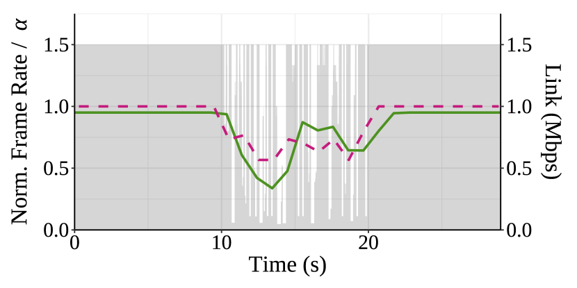
(a) $1.5\text{\,}\mathrm{M}\mathrm{b}\mathrm{p}\mathrm{s}$ link with 10s of noise and a low-motion video.

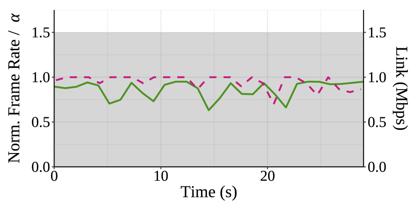
(b) Fixed $1.5\text{\,}\mathrm{M}\mathrm{b}\mathrm{p}\mathrm{s}$ link with a high-motion video.

Figure 6: $\alpha$’s response to link and video encoder variations. $\alpha$ picks lower values (more headroom) when the link capacity or encoder output varies significantly to maintain a good frame rate. The normalized frame rate is the ratio of achieved frame rate to maximum frame rate ($30\text{\,}\mathrm{F}\mathrm{P}\mathrm{S}$).

Resolution Selection. While tuning the target bitrate effectively adapts the video bitrate over smaller ranges, we change the resolution when more drastic changes are needed. Specifically, we make one of three decisions on every frame: maintain, increase, or decrease the current resolution. We decrease the resolution by one level (e.g., from 1080p to 720p) if the number of frames delivered in the last time interval $T$ is below the minimum acceptable frame rate ($5\text{\,}\mathrm{F}\mathrm{P}\mathrm{S}$ in Vidaptive) because this suggests that frames are too large for the current link capacity. In contrast, if $\alpha$ is high and the measured video bitrate is far lower than the encoder’s supplied target bitrate, the encoder is having trouble meeting its target bitrate and maintaining high utilization at the current resolution because the frames are too small. So, we increase the resolution by one level (e.g., 720p to 1080p). We simply maintain the resolution if none of the above cases are met. To avoid changing the resolution too frequently and ensure we have sufficient data points to make further changes, we only update the resolution if more than $T$ seconds have passed since the latest resolution change. The details of the mechanism are in A.2.

4 Implementation

We implemented our system on top of Google’s implementation of WebRTC [2].

Congestion Controller. We replace GCC within WebRTC with two window-based delay-sensitive algorithms, Copa [3] and RoCC [9]. We reused the logic from the original implementation of Copa [17]. Given $rtt_{min}$, the minimum observed RTT, RoCC sets the congestion window (cwnd) to a small constant more than the number of bytes received in the last $(1+\gamma)rtt_{min}$ interval. To achieve high utilization with controlled delays, RoCC aims to maintain a network queueing delay of $\gamma rtt_{min}$ where $\gamma$ is the delay-sensitiveness parameter.

Dummy Generator. We repurpose the padding generator in WebRTC to generate dummy packets that are within the cwnd and no more than 200 bytes each. Dummy packets are ACKed by the receiver but have a special padding to ensure that the payload is ignored. We have implemented safeguards to limit the maximum rate of the dummy traffic to the maximum possible video bitrate (set as $12\text{\,}\mathrm{M}\mathrm{b}\mathrm{p}\mathrm{s}$).

Latency Safeguards. The transport layer sets the encoder target bitrate to zero to signal a pause if the oldest packet’s age in the pacer queue exceeds the pacer queue pause threshold ($\tau$). We reuse WebRTC’s support for buffering the latest un-encoded camera frame. We force an Encoder Reset if the oldest packet age exceeds 1 second in Vidaptive by draining all the video packets in the pacer queue and signaling the video encoder to send a keyframe via an existing API call in WebRTC.

Encoder Rate Controller. Vidaptive has two modules to adapt the encoder to the network: encoder bitrate and resolution selection. We disabled the resolution logic in WebRTC [18] and moved the adaptation logic to occur prior to frame encoding. These modules record $\alpha$ values and frame queueing delay samples received from the transport layer whenever a frame is sent out from the pacer. Vidaptive picks the next $\alpha^{*}$ and frame resolution on a frame-by-frame basis by optimizing over the $\alpha$ and frame queueing delay values over a sliding window of the last $T$ seconds (Algorithm 1). We use $T=1$s by default. The sliding window ensures gradual changes in $\alpha$ over time.

After picking $\alpha^{*}$, the resolution module chooses whether to decrease, increase, or hold the current resolution on a per-frame basis as described in §3.4. The resolution module tracks how many consecutive frames have signaled “increase” or “decrease’ and changes the resolution if the number exceeds the threshold for that signal (15 frames for “decrease” and 30 for “increase”) . It also waits at least $T$ seconds before changing the resolution again.

5 Evaluation

We evaluate Vidaptive atop a WebRTC-based implementation on Mahimahi links. We describe our setup in §5.1 and use it to compare existing baselines in §5.2. In §5.3, we delve deeper into Vidaptive’s design components. Trace-level breakdowns of all results can be found in App. C.

5.1 Setup

Testbed. Inspired by OpenNetLab [19], we built a testbed, implemented in C++, on top of WebRTC [20] that enables a headless peer-to-peer video call between two endpoints. The sender reads video frames from an input file and the receiver records the received frames to an output file. To match video frames between the sender and the receiver for visual quality and latency measurements, a unique 2D barcode is placed on each frame [7]. We emulate different network conditions between the sender and receiver by placing the receiver behind a Mahimahi [8] link shell. Vidaptive uses Copa [3] as the default CCA. All experiments are run for $2\text{\,}\mathrm{m}\mathrm{i}\mathrm{n}$ on a lossless link with a one-way delay of $25\text{\,}\mathrm{m}\mathrm{s}$.

Metrics. Two primary metrics are used to quantify the performance improvements of Vidaptive: frame quality and frame latency. Frame quality is measured by the Peak Signal-to-Noise Ratio (PSNR [21]) between received frames and the corresponding source frames. Vidaptive reports the time between frame read at the sender and frame display at the receiver as frame latency and deems the display time for frames that are not received at the receiver as the presentation time of the subsequent displayed frame [7]. We also report the network utilization and frame rate at the receiver.

Network Traces. We evaluate each scheme on a set of 16 cellular traces bundled with Mahimahi [8], and also use synthetic traces to illustrate the convergence behavior in 10.

Videos. We use a 1080p (i.e., 1920$\times$1080) video with a frame rate of $30\text{\,}\mathrm{F}\mathrm{P}\mathrm{S}$ YUV video dataset curated from YouTube. Tab. 1 describes the details in the appendix. All the experiments are on the first video of the dataset (Tab. 1) unless stated otherwise. Audio is disabled throughout the experiments.

Baselines. We evaluate Google Congestion Control algorithm (GCC), WebRTC’s default transport mechanism. We also evaluate Vidaptive with Copa and RoCC. We use $\gamma=0.5$ (§4) for RoCC and $\delta=0.9$ (see [3]) for Copa to maintain low-network delay. We choose $\lambda=0.5$ to weigh frame rate and utilization equally when optimizing the target bitrate in Vidaptive (§3.4). The pacer queue pause threshold is set to $\tau=33ms$, and frame queueing delay measurement interval is set to $T=1s$ for online optimization of the target bitrate.

5.2 Overall Comparison

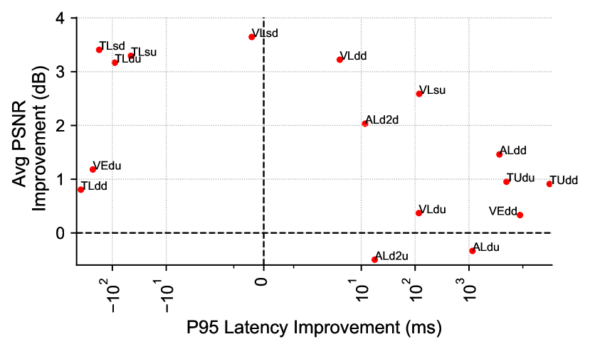
Figure 7: Average PSNR improvement vs. P95 latency improvement of Vidaptive over GCC. Vidaptive improves both P95 latency and PSNR for almost half of the traces while improving one of the two on the rest.

We summarize Vidaptive’s performance improvements over WebRTC atop GCC on all Mahimahi cellular traces in Fig. 7. The X axis (symlog [22] format) shows the P95 latency improvement, and the Y axes show the average PSNR and video bitrate improvements of Vidaptive over GCC. On nearly all traces, Vidaptive improves PSNR (1.6 dB on average). Vidaptive also improves P95 latency on 10 out of 16 traces, achieving over $2.7\text{\,}\mathrm{s}\mathrm{e}\mathrm{c}\mathrm{o}\mathrm{n}\mathrm{d}\mathrm{s}$ improvement in P95 frame latency on average across all the traces. Vidaptive has 45-380 ms higher P95 latency on 5 of the traces, although it improves average PSNR by 0.8-3.4 dB on these traces.

To better understand per-frame behavior, Fig. 8 shows the CDFs of PSNR and frame latency of all the frames across all the traces. Vidaptive achieves a better PSNR at all the percentiles by sending larger frames when possible. Overall, it improves average PSNR by $1.9\text{\,}\mathrm{d}\mathrm{B}$ and P95 PSNR by $2.2\text{\,}\mathrm{d}\mathrm{B}$. Since Vidaptive generally sends larger frames, its minimum latency is higher than GCC, and it slightly increases the median latency (148 ms for GCC versus $195\text{\,}\mathrm{m}\mathrm{s}$ for Vidaptive). However, GCC’s frame latency becomes much worse beyond the $75^{\text{th}}$ percentile. The high percentiles correspond to scenarios with high link rate variability and outages, where Vidaptive’s CCA (Copa) responds faster than GCC. For example, Vidaptive reduces P95 frame latency by $2687\text{\,}\mathrm{m}\mathrm{s}$ compared to GCC ($4120\text{\,}\mathrm{m}\mathrm{s}$ $\rightarrow$ $1433\text{\,}\mathrm{m}\mathrm{s}$).

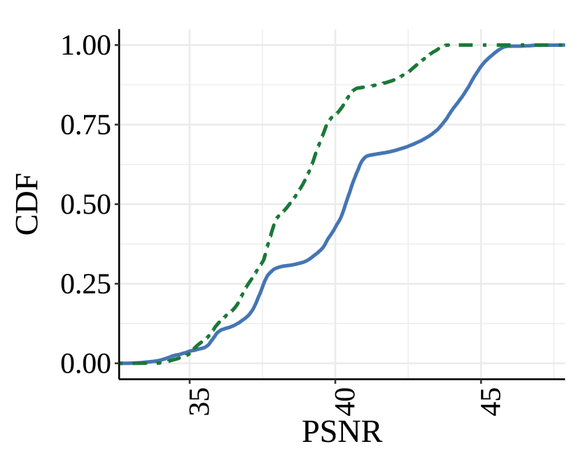
(a) PSNR CDF

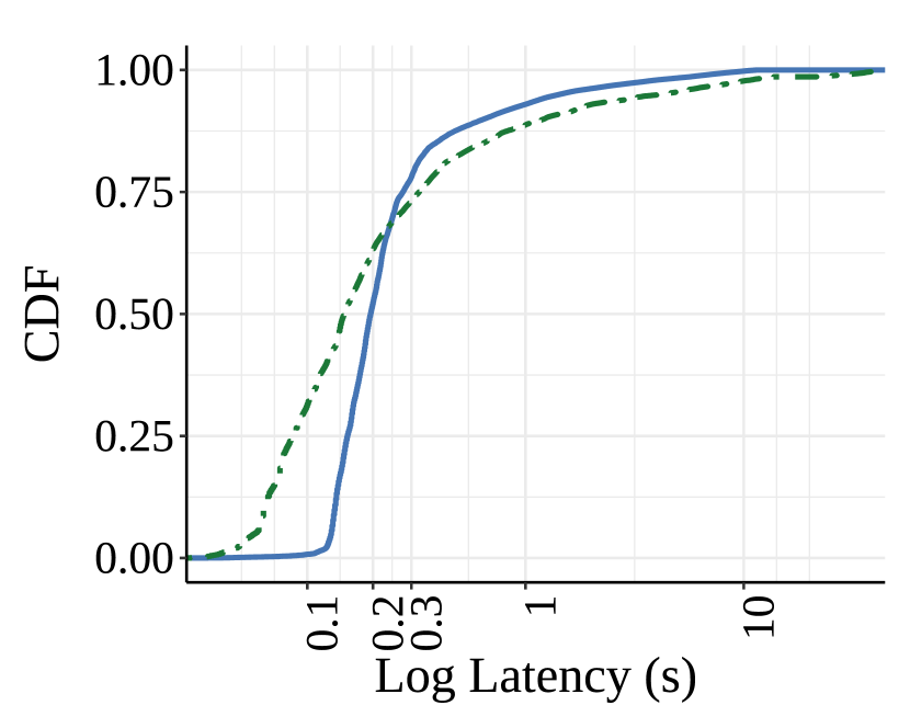
(b) Latency CDF

Figure 8: CDF of frame PSNR and latency across all frames and all the traces. Vidaptive achieves higher PSNR on all percentiles while getting lower latency on higher percentiles. Vidaptive has higher latency in lower percentiles due to larger frame sizes.

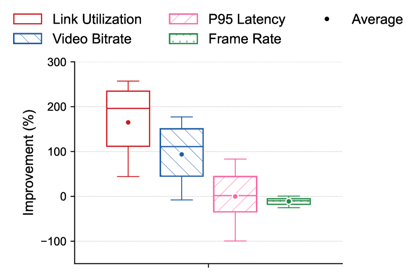
Figure 9: Performance benefits for Vidaptive over GCC. Vidaptive achieves higher utilization and video bitrate compared to GCC. Vidaptive improves P95 latency on half the traces. Vidaptive reduces the frame rate because the its CCA stops sending frames during outages to maintain low latency. The whiskers are P5 and P95, the interquartile range shows P25, P50, and P75.

Fig. 9 shows the distribution of the normalized improvement of the Vidaptive’s metrics compared to GCC per trace. The whiskers denote P5 and P95 values, the interquartile range shows P25–P75, the horizontal line shows P50 and the dot shows the average. Because Vidaptive’s CCA is more responsive, Vidaptive, on average, achieves more than $2.5\times$ of GCC’s link utilization. Vidaptive also achieves a higher video bitrate than GCC on nearly all traces, yielding an average of ${\sim}2\times$ and up to $2.7\times$ improvement. Vidaptive improves the P95 latency by up to $\sim$2x. In Fig. 7, whenever Vidaptive has a higher P95 latency, it has higher video bitrate and quality. Vidaptive has $\sim$10% and 30% lower frame rate on average and in the worst case compared to GCC, resulting in frame rates of $27\text{\,}\mathrm{F}\mathrm{P}\mathrm{S}$ and $21\text{\,}\mathrm{F}\mathrm{P}\mathrm{S}$ respectively. This reduction in frame rate happens during outages when, unlike GCC, Vidaptive’s CCA chooses not to send any frames and avoids further congestion. This caps Vidaptive’s frame rate but achieves better frame latency.

5.3 Understanding Vidaptive’s Design

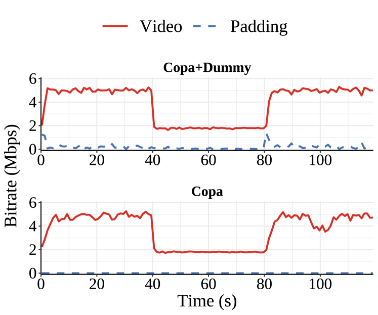
Figure 10: Copa with dummy traffic exhibits faster convergence of the video bitrate to the available network capacity and maintains a smoother steady-state video bitrate.

Effect of Dummy Traffic. To quantify the effect of dummy traffic, we disable the changes we made to the target bitrate selection logic and focus on transport layer changes (§3.2). In Fig. 10, we emulate a link that starts with $5\text{\,}\mathrm{M}\mathrm{b}\mathrm{p}\mathrm{s}$ of bandwidth for $40\text{\,}\mathrm{s}$, drops to $2\text{\,}\mathrm{M}\mathrm{b}\mathrm{p}\mathrm{s}$ for the next $40\text{\,}\mathrm{s}$ before jumping back to $5\text{\,}\mathrm{M}\mathrm{b}\mathrm{p}\mathrm{s}$. We compare the video and padding bitrate for “Copa” to Copa with dummy traffic (“Copa+Dummy”). Copa takes $6\text{\,}\mathrm{s}$ to match the network capacity, while Copa+Dummy takes $2\text{\,}\mathrm{s}$. The dummy traffic is sent only when the video traffic cannot match the link capacity when it suddenly opens up (around 0s and 80s). Copa does not match capacity as fast because its rate on the wire is determined by the slow-reacting encoder (§2). Further, “Copa+Dummy” has a more stable steady-state bitrate than “Copa” because the dummy traffic decouples the CCA’s feedback from the video encoder’s variable output, enabling more accurate link capacity estimation.

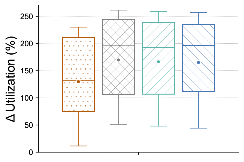
(a) Utilization improvement

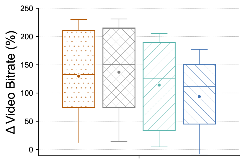
(b) Video Rate improvement

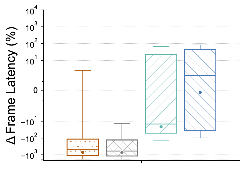
(c) P95 Latency improvement

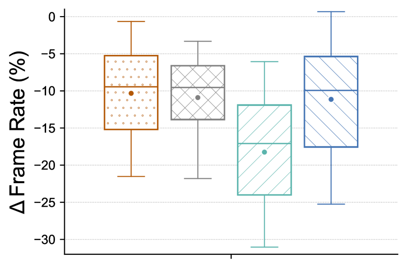
(d) Frame Rate improvement

Figure 11: Performance benefits over GCC with different Vidaptive components. “Copa” improves video bitrate and utilization but hurts frame latency. Dummy traffic improves video bitrate and utilization. Latency knobs in “Copa+Dummy+Latency” reduce the latency by seconds. With the encoder bitrate and resolution selection, Vidaptive has higher frame rate than previous versions. Since schemes with Copa do not send frames in outages, they have lower frame rate than GCC. The whiskers are P5 and P95, the interquartile range shows P25, P50, and P75.

Ablation Study. To understand the impact of different components in Vidaptive’s design, we incrementally evaluate the benefits of changing the congestion control and adding dummy traffic at the transport layer (§3.2), enabling the latency safeguards (§3.3), and running the encoder bitrate and resolution selection approach described in §3.4. Fig. 11 shows the distribution of the normalized performance improvement compared to GCC on all the traces for different system variations.

In “Copa,” we replace GCC with a window-based congestion control algorithm but keep the rest of the modules unchanged. Copa is more aggressive than GCC in bandwidth allocation, improving the average link utilization and video bitrate by over $2\times$. However, the aggressiveness causes an average increase of 3.1 seconds in the P95 latency. The frame rate also reduces because Copa’s window-based mechanism, unlike GCC, simply stops sending when it detects outages.

In “Copa+Dummy,” as the name suggests, we add dummy traffic (§3.2) on top of Copa. Since dummy traffic speeds up bandwidth discovery, the link video bitrate and link utilization improves over “Copa.” However, the P95 frame latency is still very high compared to GCC.

In “Copa+Dummy+Latency,” we enable the latency safeguards on top of “Copa+Dummy” but keep the encoder bitrate selection logic unchanged. This reduces the P95 latency (Fig. 11(c)) compared to GCC, “Copa,” and “Copa+Dummy,” yielding an average reduction of over 2.2 seconds in P95 latency compared to GCC. Since the safeguards pause encoding of frames that increase the latency, the overall frame rate, video bitrate, and utilization decrease compared to “Copa” and “Copa+Dummy.”

Finally, in “Vidaptive”, the system aims to find the right target video bitrate for the encoder by running the optimization described in §3.4. Because this system is trying to balance the frame rate and frame quality, the video bitrate reduces, and the frame rate increases compared to “Copa+Dummy+Latency”. Moreover, the latency further decreases because of the reduction of the video bitrate. The utilization is comparable across all schemes with dummy traffic since it pads any encoder output to match the link rate.

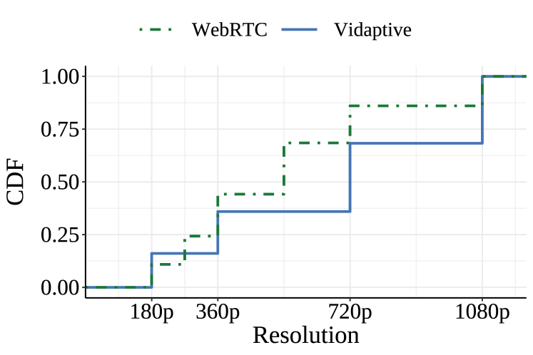
Figure 12: CDF of frame resolutions across all the traces. Vidaptive selects higher resolutions but is conservative during outages by reducing the resolution quickly in lower percentiles.

Resolution Distribution. Vidaptive uses a different resolution scheme than WebRTC. Fig. 12 shows the CDF of all the selected resolutions during the experiment across all the traces. More than 80% of the time, Vidaptive chooses a higher resolution than WebRTC, which often translates to higher video quality. When the link capacity is very low or highly variable, Vidaptive chooses to send the lowest resolution, manifesting itself in lower resolution values in low percentiles. In contrast, WebRTC’s resolution mechanism [18] reacts slowly and causes huge latency spikes. Vidaptive currently supports the resolutions shown in Fig. 12.

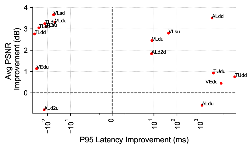
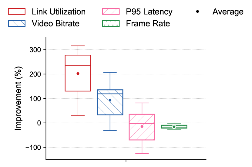
(a) Average PSNR improvement vs.P95 latency improvement of Vidaptive over WebRTC

(b) Performance improvements distribution

Figure 13: Performance of Vidaptive using a different CCA. Vidaptive (RoCC) has a similar performance to Vidaptive (Copa).

Using a Different Congestion Controller. To show that Vidaptive can work with any delay-sensitive window-based CCA, we replaced Copa with RoCC [9]. Fig. 13(b) shows the PSNR and P95 latency improvements of Vidaptive (RoCC) compared to GCC. Vidaptive (RoCC) follows similar trends as Vidaptive and improves the average video bitrate on almost all traces while improving the P95 latency for half of them. Fig. 13(b) shows the distribution of the normalized performance improvements of Vidaptive (RoCC) over GCC on all traces. Like Vidaptive, Vidaptive (RoCC) achieves a higher link utilization and video bitrate on average (more than $3\times$ and $\sim 2\times$ respectively), while getting an improvement of up to ${\sim}2\times$ in P95 latency and an increment of at most $360\text{\,}\mathrm{m}\mathrm{s}$. Vidaptive (RoCC)’s frame rate is $\sim$16% lower on average and 30% lower in the worst case than GCC, resulting in frame rates of 25 FPS and 21 FPS, respectively.

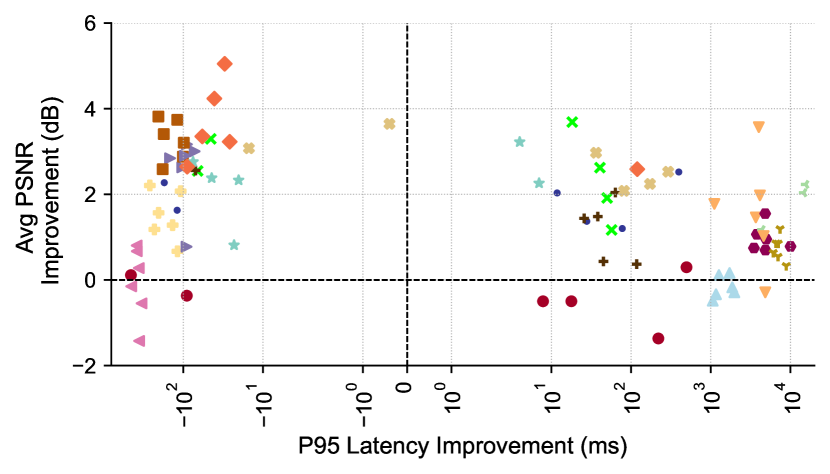
Figure 14: Average PSNR improvement vs. P95 latency improvement of Vidaptive over GCC for all the videos in the dataset. Each color denotes one trace. Vidaptive improves both P95 latency and PSNR for about half of the traces and videos while improving one of the two metrics on the rest.

Evaluation on More Videos. We evaluated Vidaptive on all the videos described in §5.1. Fig. 14 shows the average PSNR improvement against the P95 latency improvement over GCC. Vidaptive improves the average PSNR for $\sim$ 90% of the settings while increasing the P95 latency by at most $455\text{\,}\mathrm{m}\mathrm{s}$. Since Vidaptive shows similar trends for different videos, we focus on one video and Copa for the remaining experiments.

5.4 Effect of Parameter Choices

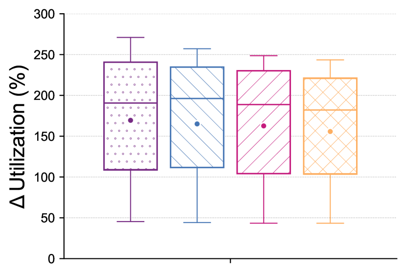
(a) Utilization improvement

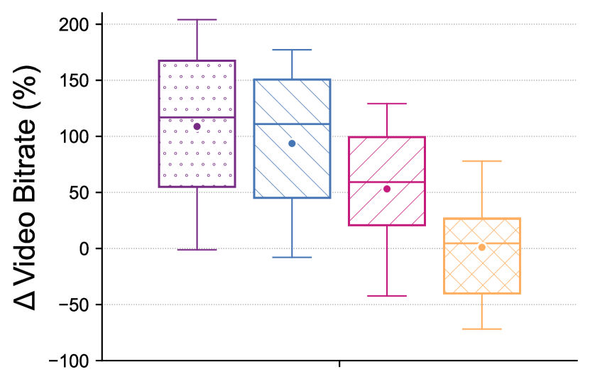
(b) Video Rate improvement

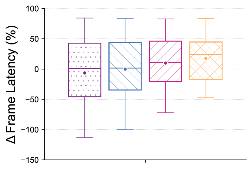
(c) P95 Latency improvement

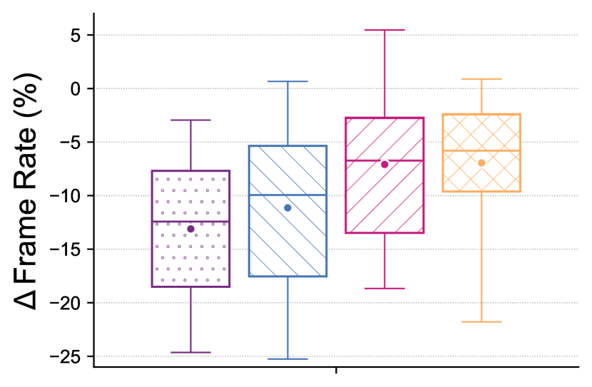
(d) Frame Rate improvement

Figure 15: Effect of $\lambda$ on Vidaptive’s performance. Increasing the value of $\lambda$ increases the frame rate and decreases the video bitrate and quality. The whiskers are P5 and P95, the interquartile range shows P25, P50, and P75.

Effect of $\lambda$. We evaluate the impact of the parameter $\lambda$, which trades off video bitrate against frame rate (§3.4). Fig. 15 shows the distribution of the normalized improvement of the metrics relative to GCC on all of the traces with $\lambda=0.2,0.5,0.7,0.99$. When $\lambda$ increases, the optimization framework in §3.4 favors a higher frame rate over the video bitrate, hence video bitrate decreases (Fig. 15(b)), and average frame rate increases (Fig. 15(d)). Since Vidaptive uses dummy traffic, changes in the video bitrate do not affect CCA estimations and consequently do not change the overall link utilization. As a result, the overall link utilization (sum of the video and padding bitrates), shown in Fig. 15(a), does not change by selecting a different $\lambda$. Vidaptive has safeguards to control the maximum latency; hence, changing $\lambda$ does not significantly affect the P95 frame latency, as seen in Fig. 15(c). Note that during any outages, Vidaptive does not send any frames, which caps Vidaptive’s frame rate. We chose $\lambda=0.5$ as the default because it maintains a good video bitrate while keeping the P95 latency low with minimal reduction in frame rate (${\sim}10\%$).

Pacer Queue Pause Threshold ($\tau$). Fig. 16 shows how the pacer queue pause threshold $\tau$ (§3.3) affects Vidaptive. We tested Vidaptive with $\tau=$ 33, 500, 1000 ms. Changing $\tau$ does not change the network utilization (Fig. 16(a)) because dummy traffic decouples congestion control from the encoder, padding any encoder output to match the link rate. As $\tau$ increases, the frame rate score increases (Eq. 1), and the encoder bitrate selection logic enforces a higher video bitrate (Fig. 16(b)). However, these higher-quality frames spend more time in the pacer queue and experience higher P95 latencies (Fig. 16(c)). At higher $\tau$, the Encoder Pause threshold is higher, so more frames are encoded, resulting in a higher frame rate (Fig. 16(d)).

Vidaptive selects $\tau=33ms$ as it has low P95 latency, relatively high frame rate and video bitrates when compared to GCC.

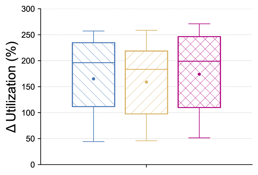
(a) Utilization improvement

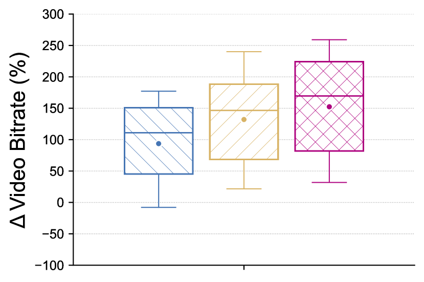
(b) Video Rate improvement

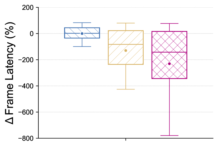
(c) P95 Latency improvement

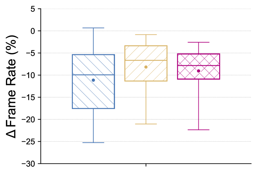
(d) Frame Rate improvement

Figure 16: Effect of pacer queue pause threshold ($\tau$) on Vidaptive. As $\tau$ increases, the P95 latency increases as frames spend a longer wait time in the pacer queue but results in higher video bitrates. Increasing $\tau$ first decreases the received frame rate as frames spend a long time in the pacer queue, but then it increases the received frame rate because Encoder Reset is triggered and new frames are encoded at lower resolution. The whiskers are P5 and P95, the interquartile range shows P25, P50, and P75.

Optimization Time Interval ($T$). We show the impact of $T$, the interval over which the frame rate and bitrate scores are calculated to strike a balance between them (§3.4). Fig. 17 shows performance improvements of Vidaptive compared to GCC for $T=100,1000,10000$ ms. Again, Vidaptive’s link utilization (Fig. 17(a)) is comparable across all variants because of dummy traffic. A smaller $T$ means that Vidaptive reacts to any sudden and local changes in recent frame queueing delay data. $T=100$ means that the encoder bitrate selection looks at utmost three measurements for a camera with $30\text{\,}\mathrm{F}\mathrm{P}\mathrm{S}$ to optimize $\alpha$. Any temporary decrease in the few frame queueing delay samples results in a higher encoder target bitrate that affects the slow encoder for a long period of time, resulting in higher video bitrate a lower frame rate and consequently a high latency. On the other hand, a large $T$ makes the system insensitive to recent changes in frame queueing delay, and a few large frame queueing delay measurements will result in lower values of $\alpha$, which reduces the video bitrate. Further, because the resolution changes at most every $T$, a $10\text{\,}\mathrm{s}\mathrm{e}\mathrm{c}\mathrm{o}\mathrm{n}\mathrm{d}$ $T$ does not lower the resolution in time in outages, causing a reduction in the frame rate and severely affecting the latency. We picked $T=1000ms$ for Vidaptive to ensure the bitrate selection is relatively stable while maintaining sensitivity to the recent frame queueing delay samples.

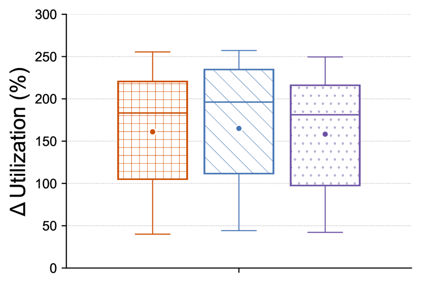
(a) Utilization improvement

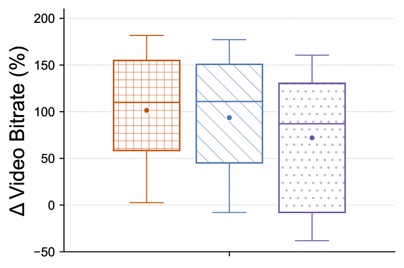
(b) Video Rate improvement

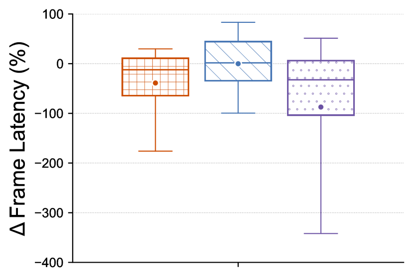
(c) P95 Latency improvement

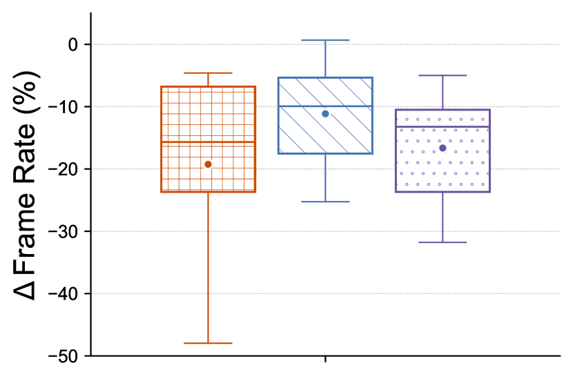
(d) Frame Rate improvement

Figure 17: Performance comparison of Vidaptive using different intervals $T$, for encoder bitrate selection. The duration of $T$ affects the sensitivity to recent frame queueing delay measurements, and consequently the frame rate, latency and video bitrate of the system. The whiskers are P5 and P95, the interquartile range shows P25, P50, and P75.

6 Related Work

Congestion Control. End-to-end congestion control approaches can be broadly categorized into delay-based [10, 3, 23, 24, 25, 6, 1, 4] or buffer-filling schemes [26, 27]. Delay-based protocols aim to minimize queuing by adjusting their sending rate based on queuing delay [28, 25, 10], or delay-gradients [1, 6, 24]. Buffer-filling algorithms [26, 29, 30] send as much traffic as possible until loss or congestion is detected. Some approaches like Nimbus [31] switch between delay-based and buffer-filling modes to improve fairness against competing traffic while maintaining high utilization. However, limited attention has been paid to congestion control for application-limited flows [32, 33] like video traffic that is generated at fixed intervals determined by the frame rate.

WebRTC Systems. Many video applications use Web Real-time Communication (WebRTC) [2] to deliver real-time video. GCC [34], WebRTC’s rate control, uses delay gradients to adjust the sending rate. However, GCC’s conservative behavior coupled with the variance in encoder output results in either under-utilization or latency spikes.

Salsify [7] previously observed a mismatch between video encoder output and available capacity, and rectified it by encoding multiple versions of the same frame and picking the better match. This requires changing the video codec at the sender and the receiver, making it hard to deploy. Vidaptive instead matches encoder output to network capacity without changes to the encoder. Adaptive bitrate algorithms [35, 36, 37, 38, 39] solve a similar problem for on-demand video using information about available bandwidth, buffer size, and current bitrate to determine the encoder’s target bitrate. A recent proposal called SQP [40] achieves low end-to-end frame delay for interactive video streaming applications but operates in much higher bitrates than Vidaptive is designed for.

7 Conclusion

This paper proposes Vidaptive, a new rate control mechanism for low-latency video applications that is highly efficient and adapts rapidly to changing network conditions without modifications to the video encoder. Vidaptive injects “dummy” traffic to make video traffic appear like a backlogged flow running a delay-based congestion controller. Vidaptive also continuously adapts the frame rate, encoder’s target bitrate, and video resolution to reduce discrepancies between the encoder output bitrate and link rate. We leave to future work an exploration of leveraging dummy traffic for purposes like FEC or keyframes, and the benefits from functional encoders like Salsify [7] in Vidaptive for improved real-time experience.

Appendix A Encoder Bitrate and Resolution Selection Mechanism

In this section, we explain the encoder bitrate and resolution selection algorithms in detail.

A.1 Solving the Optimization Problem

Assume we have $N$ frame queueing delay measurements $d_{i}$ for $i\in\{1,2,..,N\}$ over a time interval $T$, for frames encoded instantaneously with a target bitrate $\alpha_{i}\cdot\text{{\tt CC-Rate}}$ where CC-Rate was approximated to be constant over the interval. We use hindsight optimization and ask “had we picked a different target bitrate, what would have been the counterfactual values of $d_{i}$?” We use $\tilde{.}$ to show counterfactual variables.

Had all these frames been encoded by $\alpha$ instead, the counterfactual frame queueing delay would have been $\tilde{d_{i}}=\alpha\frac{d_{i}}{\alpha_{i}}$. Let $k_{i}=\frac{d_{i}}{\alpha_{i}}$ for $i\in\{1,2,..,N\}$. The counterfactual values of $\mathcal{F}$ and $\mathcal{B}$ as a function of $\alpha$ are

$$\tilde{\mathcal{F}}(\alpha) =\frac{\sum_{i=1}^{N}\mathbb{1}[\alpha\cdot\frac{d_{i}}{\alpha_{i}}\leq\tau]}{N}$$ (4)

$$=\frac{\sum_{i=1}^{N}\mathbb{1}[\alpha\cdot k_{i}\leq\tau]}{N}$$

$$\tilde{\mathcal{B}}(\alpha) =min\Big{(}f_{max}\cdot\frac{\sum_{i=1}^{N}\alpha\cdot\frac{d_{i}}{\alpha_{i}}}{N},1\Big{)}$$ (5)

$$=min\Big{(}f_{max}\cdot\frac{\sum_{i=1}^{N}\alpha\cdot k_{i}}{N},1\Big{)}$$

With this definition, we find $\alpha^{*}$ such that it maximizes the counterfactual optimization objective, denoted by $\text{Objective}(\alpha)$,

$$\alpha^{*} =\operatorname*{arg\,max}_{\alpha}\quad\text{Objective}(\alpha)$$ (6)

$$=\operatorname*{arg\,max}_{\alpha}\quad\frac{\lambda}{1-\lambda}\tilde{\mathcal{F}}(\alpha)+\tilde{\mathcal{B}}(\alpha)$$

$$=\operatorname*{arg\,max}_{\alpha}\left\{\frac{\lambda}{1-\lambda}\frac{\sum_{i=1}^{N}\mathbb{1}[\alpha\cdot\frac{d_{i}}{\alpha_{i}}\leq\tau]}{N}\right.$$

$$\left.\phantom{=\operatorname*{arg\,max}_{\alpha}\quad}+\min\Big{(}f_{max}\cdot\frac{\sum_{i=1}^{N}\alpha\cdot\frac{d_{i}}{\alpha_{i}}}{N},1\Big{)}\right\}$$

s.t. $$0<\alpha<1$$

Without loss of generality, we assume that the values of $k_{i}$ for $i\in\{1,2,...,N\}$ are sorted in increasing order. Let $x_{i}=\frac{\tau}{k_{i}}$ for $i\in\{1,2,...,N\}$. Note that $x_{i}$ values are in decreasing order. $\tilde{\mathcal{F}}(\alpha)$ is a discrete monotonically reducing function relative to $\alpha$ whose value changes at $\alpha=min(\frac{\tau}{k_{i}},1)$ for $i\in\{1,2,...,N\}$. If $x_{i+1}<x_{i}$ we have $\tilde{\mathcal{F}}(x_{i+1})=\tilde{\mathcal{F}}(x_{i})+1$ for $0<x_{i},x_{i+1}<1$. Since $\tilde{\mathcal{B}}(\alpha)$ is a monotonically increasing function of $\alpha$, we have $\tilde{\mathcal{B}}(x_{i+1})<\tilde{\mathcal{B}}(x_{i})$. For any value of $x$ such that $x_{i+1}<x\leq x_{i}$, since $\tilde{\mathcal{F}}(x)=\tilde{\mathcal{F}}(x_{i})$ and $\tilde{\mathcal{B}}(x)\leq\tilde{\mathcal{B}}(x_{i})$, $\text{Objective}(x)\leq\text{Objective}(x_{i})$. As a result, checking $\text{Objective}(x_{i})$ and $\text{Objective}(x_{i+1})$ is enough to find the maximum in interval $(x_{i+1},x_{i}]$. This means that checking $x_{i}$ values for $i\in\{1,2,...,N\}$ is sufficient to find $\alpha^{*}$. Algorithm 1 shows the detailed algorithm for solving this optimization problem. In our implementation, if $N$ is not large enough, we declare an outage and linearly increase the amount of $\alpha$ to back off from the congestion.

A.2 Resolution Selection Mechanism

Vidaptive has an adaptive mechanism to change the resolution in two scenarios. First, when the current frame rate is low, Vidaptive lowers the resolution because the current frame sizes are too big to go through the network. Second, if the output average video bitrate of the encoder is lower than the average target bitrate given to the encoder in the last $T$ seconds, despite a high $\alpha^{*}$, Vidaptive needs to increase the resolution because the encoder is unable to match the current bitrate at its current resolution. The assumption behind this is that if the chosen resolution for the encoder is correct, the encoder should be able to achieve its target bitrate over long periods of time (e.g. $T=1000ms$). The resolution selection module sits before the video encoder to choose the resolution on a frame-by-frame basis. It also observes the output of the encoder to measure the video bitrate. It measures the system’s current frame rate and its enc_ratio, the ratio between the encoder’s achieved bitrate and its supplied target bitrate. We define MinFrameRate as the minimum acceptable frame rate of the system, and MinEncRatio as the minimum required value of enc_ratio. The resolution selection module decides on a per-frame basis to emit a “Decrease”, “Increase” or “Hold resolution” signal based on the values of its measurements as described in Algorithm 2.

If Vidaptive releases “Decrease Resolution” for ResDownThresh, set to 15 consecutive frames, the frame rate has been consistently low and the resolution is decreased. If Vidaptive releases “Increase Resolution” for ResUpThresh, set to 30 consecutive frames, the encoder is not keeping up with the target bitrate for a long period and the resolution is increased. We also prevent unwanted resolution oscillations that could adversely affect the quality of experience by making sure we don’t change resolution twice within a time interval of $T$.

Input :  D: Vector of frame queuing delays,
A: Vector of $\alpha$ values for frames in D,
$\alpha^{\prime}$: Current value of $\alpha$

Output :  $\alpha^{*}$: encoder bitrate ratio to CC-Rate

// Control Parameters

$f_{max}\leftarrow 30$ ;

  // max. frame rate of system

$\lambda\leftarrow 0.5$ ;

  // Frame rate sensitivity

$\tau\leftarrow 33$ ;

  // Frame Drop Threshold

$T$ ;

  // Optimization interval (s)

$\text{MinFrameRate}\leftarrow 5$ ;

  // Min. frame rate (FPS)

$\alpha_{min}\leftarrow 0.05$ ;

  // Min. $\alpha$ value

$\alpha_{max}\leftarrow 1.0$ ;

  // Max. $\alpha$ value

Function Objective($x$, $K$):

      $N=\text{Size}(\text{D})$;

     

     $\mathcal{F},\mathcal{B}=0,0$;

      for $i\leftarrow 0$ to $N-1$ do

           $\mathcal{B}\leftarrow\mathcal{B}+\frac{K[i]}{N}$ if $K[i]\leq\tau$  then

                $\mathcal{F}\leftarrow\mathcal{F}+\frac{1}{N}$

               

                $\mathcal{B}\leftarrow\min(\mathcal{B},1)$ return $\frac{\lambda}{1-\lambda}\mathcal{F}+\mathcal{B}$

               

               Function FindAlpha ($D$, $A$, $\alpha^{\prime}$):

                    

                    $N=\text{Size}(\text{D})$;

                    

                    if $\frac{N}{T}\leq\text{MinFrameRate}$ then

                         // Not enough samples, frame rate is small

                         // Frames too big return $max(\alpha^{\prime}-0.15,\alpha_{min})$

                         

                         $K\leftarrow$ empty list;

                         

                         for $i\leftarrow 0$ to $N-1$ do

                               $K[i]\leftarrow\frac{D[i]}{A[i]}$;

                              

                              

                              Sort K in ascending order;

                              

                              $\alpha^{*}\leftarrow\alpha_{max}$;

                              

                              $\text{max\_obj}\leftarrow$ Objective ($\alpha_{max},\text{K}$)

                              for $i\leftarrow 0$ to $N-1$ do

                                    if $\frac{\tau}{\alpha_{max}}<\text{K}[i]\leq\frac{\tau}{\alpha_{min}}$ then

                                        $\text{x}\leftarrow\frac{\tau}{\text{K}[i]}$;

                                        

                                        $\text{obj\_value}\leftarrow\textnormal{{Objective(}}\textnormal{\emph{\text{x}, \text{K}}}\textnormal{{)}}$;

                                        

                                        if $\text{max\_obj}<\text{obj\_value}$ then

                                              $\text{max\_obj}\leftarrow\text{obj\_value}$;

                                             

                                             $\alpha^{*}\leftarrow\text{x}$;

                                             

                                             

                                             

                                              return $\alpha$

Algorithm 1 Solving Optimization to Find Encoder Target Bitrate Ratio ($\alpha^{*}$)

// Control Parameters
$\text{T}\leftarrow 1$ ;

  // Optimization interval (s)

$\text{MinEncRatio}\leftarrow 0.9$ ;

  // Min. required encoder ratio

$\text{MinFrameRate}\leftarrow 5$ ;

  // Min. frame rate (FPS)

$\text{ResUpThresh}\leftarrow 30$ ;

  // Approx. 1 second

$\text{ResDownThresh}\leftarrow 15$ ;

  // Approx. 500 ms for outage

// Global Parameters
$\text{PrevSignal}\leftarrow 0$ ;

  // previous res. signal

$\text{SignalCount}\leftarrow 0$ ;

  // # of consecutive res. signals

$\text{LastResTime}\leftarrow 0$ ;

  // Last res. change time (s)

$\text{DecRes}\leftarrow-1$ ;

  // Decrease Resolution

$\text{HoldRes}\leftarrow 0$ ;

  // Hold Resolution

$\text{IncRes}\leftarrow-1$ ;

  // Increase Resolution

Input :  $N$: Number of frame queuing delay samples,

$\alpha^{*}$: Current value of $\alpha$,

enc_ratio: encoder output to input bitrate ratio,

now: Time in s when calling the function

Output :  res_dir: Direction to change the resolution

$\text{res\_dir}\leftarrow\text{HoldRes}$

if $\frac{N}{T}\leq\text{MinFrameRate}$ then

      $\text{res\_signal}\leftarrow\text{DecRes}$

      else if $\text{enc\_ratio}<\text{MinEncRatio}$ and $\alpha^{*}>0.9$ then

           $\text{res\_signal}\leftarrow\text{IncRes}$

          

          if $\text{res\_signal}=\text{PrevSignal}$ and $\text{res\_signal}\neq 0$ then

                $\text{SignalCount}\leftarrow\text{SignalCount}+1$

                else

                     $\text{SignalCount}\leftarrow 0$

                    

                    $\text{PrevSignal}\leftarrow\text{res\_signal}$

                    if $\text{LastResTime}<\text{now}-T$ then

                          if $\left(\text{SignalCount}>\text{ResDownThresh}\textbf{ and }\text{res\_signal}=\text{DecRes}\right)$ or $\left(\text{SignalCount}>\text{ResUpThresh}\textbf{ and }\text{res\_signal}=\text{IncRes}\right)$ then

                               $\text{LastResTime}\leftarrow\text{now\_ms}$

                              $\text{SignalCount}\leftarrow 0$;

                              

                              $\text{res\_dir}\leftarrow\text{res\_signal}$

                               else

                                    $\text{res\_dir}\leftarrow\text{HoldRes}$

                                   

                                   

                                   return res_dir

Algorithm 2 Adaptive Resolution Control

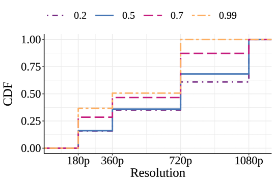
Figure 18: CDF of all frame resolutions across all the traces for different values of $\lambda$. As $\lambda$ increases, Vidaptive becomes more conservative in selecting higher resolutions.

Appendix B Video Bitrate Improvements

Figures 19(a), 19(b), and 19(c) show the corresponding video bitrate vs. latency improvements for experiments shown in Figures 7, 13, and 14.

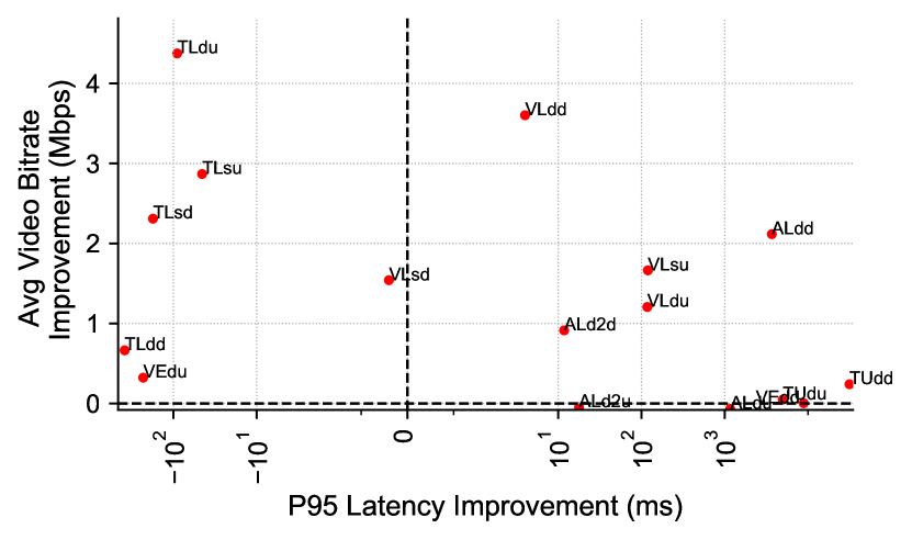
(a) Average Video Bitrate improvement vs P95 latency improvement of Vidaptive over GCC.

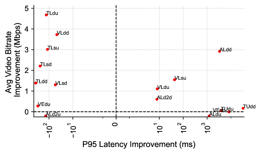
(b) Avg. video bitrate improvement vs. P95 latency improvement of Vidaptive (RoCC) over GCC.

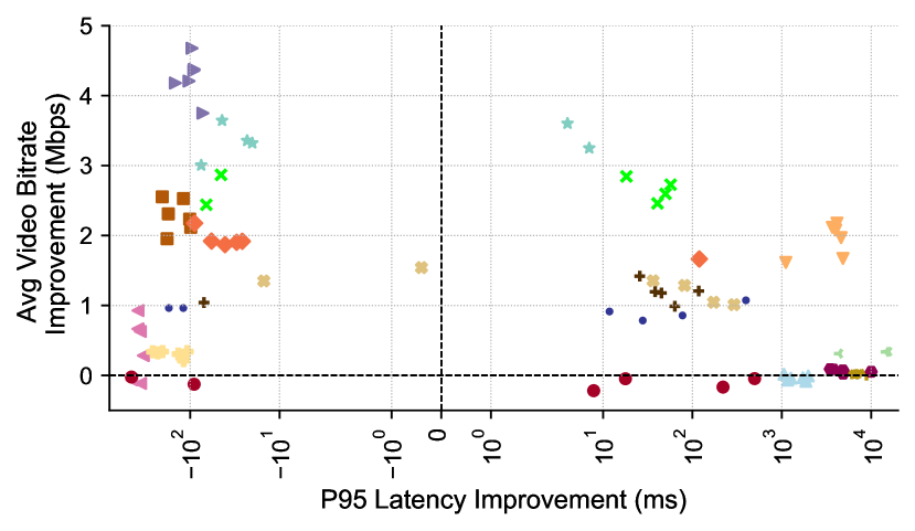
(c) Average video bitrate improvement vs. P95 latency improvement of the Vidaptive over GCC for individual videos in the dataset.

Figure 19: Corresponding video bitrate vs. latency improvements for experiments in §5.

Appendix C Trace-level Breakdown of Results

Overall Results. Fig. 20 shows a detailed comparison of end-to-end frame metrics and video bitrate of GCC, Vidaptive, and RoCC+Vidaptive on all the cellular traces. The whiskers denote P5 and P95 values, the interquartile range shows P25–P75, the horizontal line shows P50 and the dot shows the average. Fig. 20(a) describes the distribution of frame PSNRs. The average and median PSNR achieved by Copa and RoCC is higher than GCC on nearly all traces. Moreover, the best frames in Vidaptive (P75 and P95) have a much higher quality compared to GCC; e.g., Vidaptive achieves PSNR of more than $44\text{\,}\mathrm{d}\mathrm{B}$ in VLdd.

On these highly variable cellular links, Vidaptive spans a wider range of qualities because its adaptive resolution and fast CCA can capture opportunities to send at higher bitrates, increasing the PSNR average and P95 values, while reacting fast to outages by lowering the encoder target bitrate. For example, in TUdd and TUdu, Vidaptive trades off lower bitrate and worse P5 and P25 frame PSNR relative to GCC for better P95 and P75 frame latency (Fig. 20(b)) by reacting faster during outages.

However, if the link is generally more stable, Vidaptive’s worst frames (P5 and P25) have better or comparable quality than GCC, such as on TLsu. Though Copa and RoCC control network delays differently, their latency values (Fig. 20(b)) show similar trends because the latency safeguards within Vidaptive are set up to bound latency independent of the congestion control dynamics. The P5 and P95 values of the latency for Vidaptive are generally higher because it prioritizes higher quality frames. Fig. 21(a) shows that Vidaptive has a higher video bitrate and link utilization (sum of the video and dummy traffic) than GCC. GCC’s lower P5 and P95 latency is also partially attributed to this under-utilization relative to Vidaptive.

Vidaptive generally has a slightly lower frame rate as shown in Fig. 20(c) because Copa and RoCC do not send the video frames out on wire if the network is congested. In such cases, Vidaptive pauses the encoder to keep the latency bounded. However, Vidaptive still obtains a good frame rate of more than $20\text{\,}\mathrm{F}\mathrm{P}\mathrm{S}$ on almost all the traces, which is sufficient for most real-time video applications. On three challenging traces - TUdd, TUdu, VEdd - all the schemes have difficulty maintaining a good frame rate.

Fig. 21(b) shows the distribution of the instantaneous link utilization measured using Mahimahi logs. The instantaneous utilization is the ratio of the departure rate of the link to the actual link capacity. Vidaptive has a higher average and median instantaneous link utilization than GCC on all the traces with both RoCC and Copa. The reason is that using the dummy traffic enables isolation of the congestion controllers and the video traffic, and the congestion controllers can now freely estimate and utilize the network well.

Fig. 21(c) breaks down the distribution of in-network delay for the schemes. The difference between network delay and frame latency is that network delay measures the packet delays inside the network, but frame latency measures an end-to-end metric between frame read and frame display time. If the network delay that the video packets experience is high, the frame latency associated with that frame will inevitably be high. Vidaptive’s delay-sensitive algorithms ensure that in nearly all the traces, Vidaptive consistently maintains low network delay. GCC, in contrast, has a higher network delay on most traces because it does not have a mechanism to control queues in the network effectively. This is especially true on TUdd, TUdu, and VEdd, where GCC experiences high network delays and frame latencies.

Since Copa slightly outperforms RoCC relative to GCC, we set Copa as the default CCA in Vidaptive.

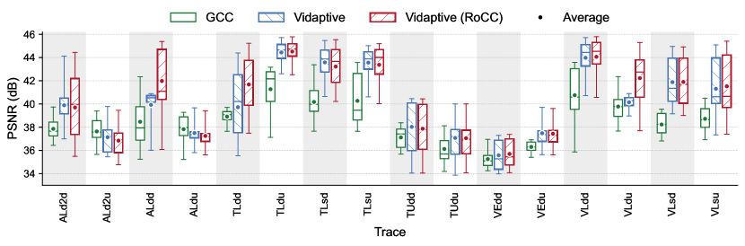
(a) Per-frame PSNR statistics comparison of the received video vs. the original video. Vidaptive has better PSNR values compared to GCC on almost all the traces.

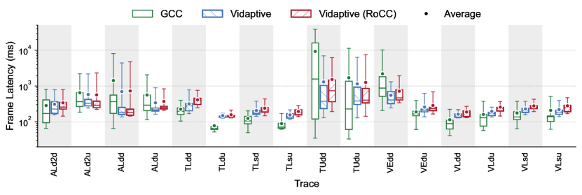
(b) Per-frame latency statistics comparison of the received video vs. the original video. Vidaptive has a comparable (within less than $400\text{\,}\mathrm{m}\mathrm{s}$ of GCC) or much lower latency values compared to GCC.

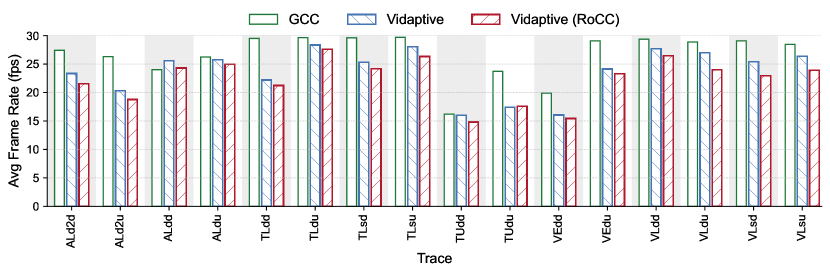
(c) Average frame rate

Figure 20: Comparison of end-to-end frame statistics of quality of experience metrics of Original GCC, Vidaptive, and Vidaptive (RoCC) on all the Mahimahi cellular traces. Vidaptive has higher quality than GCC on all traces and either improves one or both amongst PSNR or P95 latency. Vidaptive on average has lower received frame rate. The whiskers are P5 and P95, the interquartile range shows P25, P50, and P75, and the dot shows the average.

(a) Average throughput of Video traffic vs. Dummy traffic for different schemes. Vidaptive sends a higher video bitrate and an overall higher link utilization on almost all the traces.

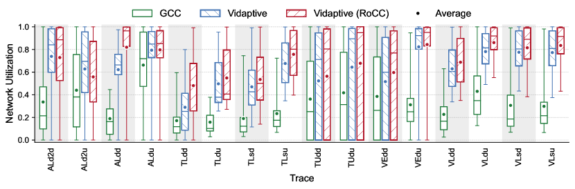
(b) Instantaneous link utilization distribution for all the schemes. Vidaptive’s average and median instantaneous link utilization of the network is higher than GCC on all the traces.

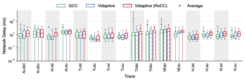
(c) In-network queueing delay distribution for all the schemes. Vidaptive has network delay-sensitive CCA that strives to keep the queueing delay low, while GCC has higher network delay in most traces.

Figure 21: Comparison of network statistics of Original GCC, Vidaptive, and Vidaptive (RoCC) on all the Mahimahi cellular traces. Vidaptive has a higher average and a higher median and average instantaneous utilization than GCC. Vidaptive has a more controlled network delay and is lower on most traces. The whiskers are P5 and P95, the interquartile range shows P25, P50, and P75, and the dot shows the average.

Effect of $\lambda$. Fig. 22(a) shows the distribution of PSNR values for different values of $\lambda$. As $\lambda$ increases, the optimization in Eq. 3 favors a higher frame rate (Fig. 22(c)) to a lower video bitrate(Fig. 23(a)). As $\lambda$ increases, Vidaptive becomes more and more conservative by choosing lower values of $\alpha$ which results in choosing lower resolutions that cap the maximum quality as $\lambda$ increases (P95 values of quality decreases). Fig. 18 shows the CDF of the resolutions selected by Vidaptive for all the frames in all the traces. Lower resolution also reduces the average, median, and P25 values of PSNR. As $\lambda$ increases, Vidaptive becomes more conservative in selecting higher resolutions. Fig. 22(b) shows that the latency measurements generally come down by increasing $\lambda$. Simultaneously, the video bitrates and resolution become lower.

Fig. 22(c) shows that the average frame rate increases as $\lambda$ increases, exactly as we designed it to. Using dummy traffic decouples the CCA estimations from the underlying video traffic; hence, the distribution of instantaneous link utilization (Fig. 23(b)) and network queueing delay (Fig. 23(c)) are agnostic for different values of $\lambda$. The sum of the total average video bitrate and dummy traffic (total link utilization) is constant for different values of $\lambda$ (Fig. 23(a)).

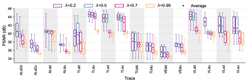
(a) Demonstrating the effect of $\lambda$ on the PSNR. When $\lambda$ increases, the average PSNR decreases as a result of the reduction in video bitrate.

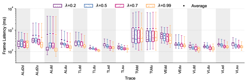
(b) Demonstrating the effect of $\lambda$ on the latency. Vidaptive has safety guards to control the maximum latency; hence, $\lambda$ does not significantly affect the P95 frame latency. However, it reduces other latency measurements as Vidaptive gets more conservative.

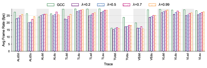
(c) Demonstrating the effect of $\lambda$ on the average frame rate, when $\lambda$ increases, the optimization problem in Eq. 3 favors a higher frame rate over the video bitrate, hence the frame rate increase.

Figure 22: Displaying the effect of $\lambda$ on end-to-end frame metrics of quality of experience. As $\lambda$ increases, the PSNR decreases but the frame rate increases. The average and median latency decreases as Vidaptive becomes more conservative. The whiskers are P5 and P95, the interquartile range shows P25, P50, and P75, and the dot shows the average.

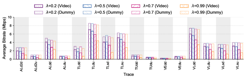
(a) Demonstrating the effect of $\lambda$ on the Video and Dummy bitrate. When $\lambda$ increases, the optimization problem in Eq. 3 favors a higher frame rate over the video bitrate; hence video bitrate decreases. The total sum of dummy and video traffic remains constant.

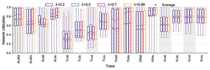
(b) Instantaneous link utilization distribution for different $\lambda$. Vidaptive has an almost identical distribution of instant link utilization because of the decoupling of CCA and video.

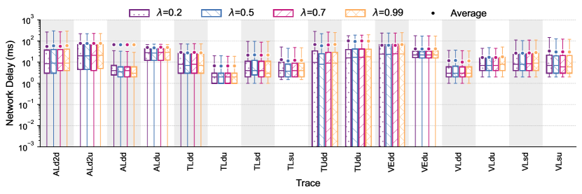
(c) In-network queueing delay distribution for different $\lambda$. Vidaptive has an almost identical distribution of network delay.

Figure 23: Comparison of network statistics of Vidaptive using different values of $\lambda$. Vidaptive has similar network characteristics and simulates the behavior of a backlogged flow from the network’s perspective. The whiskers are P5 and P95, the interquartile range shows P25, P50, and P75, and the dot shows the average.

Ablation Study. Fig. 24 compares the frame statistics of the systems described in the ablation study in §5.3. Adding the dummy traffic to “Copa”, “Copa+Dummy” achieves a slightly higher link utilization (Fig. 25(b)) because the added dummy traffic enables better estimation of the network by providing traffic when there are no video packets. Having a better network estimation helps increase the average video bitrate (Fig. 25(a)) and video quality (Fig. 24(a)) across its entire range. For “Copa” and “Copa+Dummy”, the PSNR values increase (Fig. 24(a)) and the link utilization (Fig. 25(b)) increases compared to GCC, and the average video bitrate (Fig. 25(a)) goes up consequently because Copa is much more aggressive with estimating the link rate and giving the highest possible bitrate (Fig. 25(a)) to the encoder. However, without Vidaptive latency knobs, “Copa” and “Copa+Dummy” experience very high latency values because there is no mechanism to control the size of the pacer queue when the encoder is producing such high bitrates and the network is congested, and CCA is not sending.

To fix this issue, “Copa+Dummy+Latency” uses the latency mechanisms of Encoder Pause and Encoder Reset that reduce the latency values across its range (Fig. 24(b)), but lowers the frame rate as a consequence of Encoder Pause. Since “Copa+Dummy+Latency” encodes fewer frames, it has a lower video bitrate (Fig. 25(a)) and consequently lower quality (Fig. 24(a)) than the variations without “Latency”. The network delay and instantaneous utilization distributions are almost identical to “Copa+Dummy” since we using dummy traffic. To fix the issue with lower frame rate, Vidaptive adds the optimization mechanism in §3.4. The increase in frame rate and decrease in the video bitrate can be seen in and Fig. 24(c) Fig. 25(a), respectively.

All the variations that have Copa as the underlying CCA, keep the network delay bounded (Fig. 25(c)) on all traces because Copa is delay-sensitive. They also have a similar network delay and instantaneous utilization distribution for each trace. These variations prioritize the network delay and don’t send any traffic during outages, which restricts the frame rate of the systems that use them (Fig. 24(c)), meaning that the system prefers to skip encoding the frames that much increase the total number of bytes in flight.

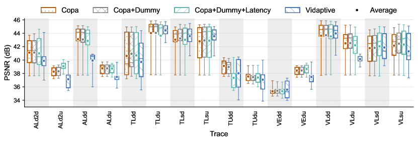
(a) Per-frame PSNR statistics comparison of the received video vs. the original video for different system variations.

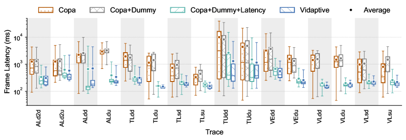
(b) Per-frame latency statistics comparison of the received video vs. the original video for different system variations. Vidaptive has lower latency percentiles because of the smarter mechanism adjusts the encoder bitrate.

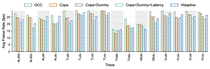
(c) Average frame rate comparison across different system variations. Vidaptive achieves a good frame rate while maintaining the latency.

Figure 24: Comparison of end-to-end frame statistics of quality of experience metrics for different system variations. Vidaptive gets the best trade-off between latency, PSNR, and frame rate compared to GCC across all the variations. The whiskers are P5 and P95, the interquartile range shows P25, P50, and P75, and the dot shows the average.

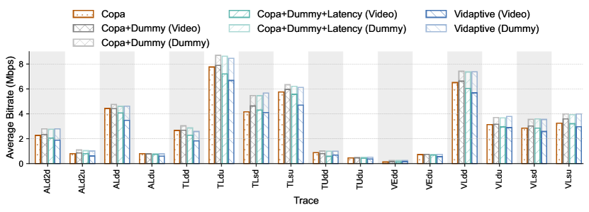
(a) Average throughput of Video traffic vs. Dummy traffic for different system variations. Vidaptive obtains the best balance between the video bitrate and link utilization among all the variation.

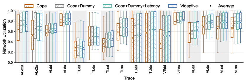
(b) Instantaneous link utilization distribution for all the system variations. All the systems with the dummy traffic have similar link utilization distribution. Adding the dummy traffic to “Copa” increases all the percentiles for the link utilization.

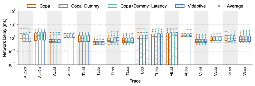
(c) In-network queueing delay distribution for all the schemes. All the variations have similar distributions.

Figure 25: Comparison of network statistics of system variations on all the Mahimahi cellular traces. All the variations using the dummy traffic display almost identical behavior network behaviors.

Details of Effect of Pacer Queue Threshold ($\tau$). Fig. 26 shows the comparison of quality-of-experience metrics for different values of $\tau$. Although changing $\tau$ doesn’t affect the network utilization due to dummy traffic, increasing it will result in a higher frame-rate score and, ultimately, a higher video bitrate. As shown in Fig. 26(a), this translates to higher frame quality for most of the traces. At the same time, as frame sizes increase, we experience higher latency (Fig. 26(b)). Since higher values for $\tau$ mean less aggressive pausing of the encoder, we also experience a higher frame rate.

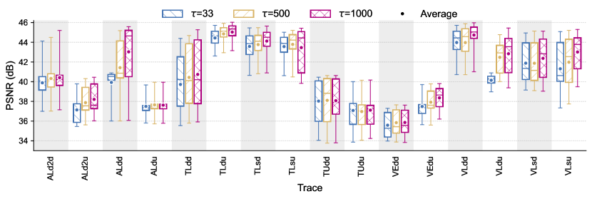
(a) Per-frame PSNR statistics comparison for different pacer queue thresholds ($\tau$). Increasing $\tau$ increases $\alpha$ in Eq. 3, which increases the video bitrate and quality.

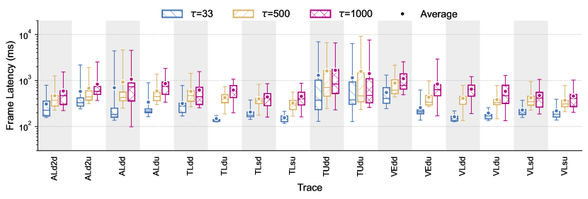
(b) Per-frame latency statistics comparison for different pacer queue thresholds ($\tau$). Increasing $\tau$ eases the Encoder Pause mechanism and increases the latency.

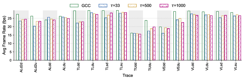
(c) Average frame rate for different pacer queue thresholds ($\tau$). Increasing $\tau$ pauses fewer frames but increases the latency, so the exact effect of on average frame rate depends on the link characteristics.

Figure 26: Comparison of end-to-end quality-of-experience metrics for different values of $\tau$ on all the Mahimahi cellular traces.

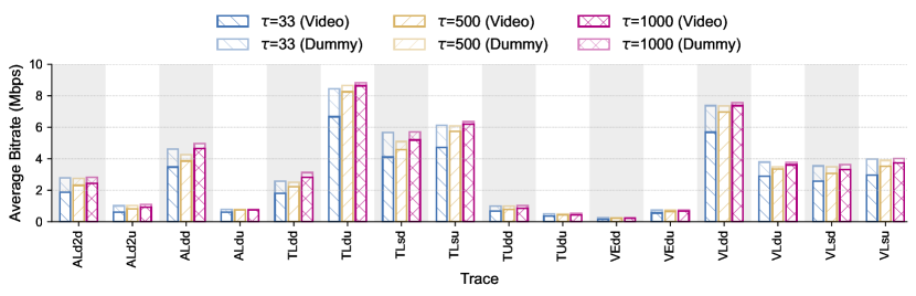
(a) Average throughput of Video traffic vs. Dummy traffic for different pacer queue thresholds ($\tau$). A higher pacer queue threshold increases the frame rate score, increasing the $\alpha$ and consequently the video bitrate.

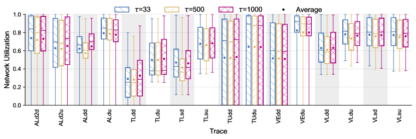
(b) Instantaneous link utilization distribution for different pacer queue thresholds ($\tau$). Using the dummy traffic, the link utilization is agnostic to the underlying video traffic.

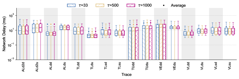
(c) In-network queueing delay distribution for different pacer queue thresholds ($\tau$). Using the dummy traffic, the CCA decisions are independent of the video traffic, so the network delay is agnostic to $\tau$.

Figure 27: Comparison of network statistics for different values of $\tau$. Vidaptive has similar network characteristics and simulates the behavior of a backlogged flow from the network’s perspective. The whiskers are P5 and P95, the interquartile range shows P25, P50, and P75, and the dot shows the average.

Appendix D Videos

Dataset Information Tab. 1 summarizes the information of all the videos that we used in the experiments. The videos are all collected from YouTube and cover a different range of motions and settings.

	Videos
Youtuber	Total Len.	Avg. Bitrate
Video 1	10 min	2521 kbps
Video 2	10 min	1082 kbps
Video 3	10 min	2815 kbps
Video 4	10 min	2013 kbps
Video 5	3 min	1694 kbps

Table 1: Details of our dataset. All videos are at 1920$\times$1080.

References

- [1] Gaetano Carlucci, Luca De Cicco, Stefan Holmer, and Saverio Mascolo. Analysis and design of the google congestion control for web real-time communication (webrtc). In Proceedings of the 7th International Conference on Multimedia Systems, pages 1–12, 2016.
- [2] WebRTC. https://webrtc.org/.
- [3] Venkat Arun and Hari Balakrishnan. Copa: Practical delay-based congestion control for the internet. In 15th USENIX Symposium on Networked Systems Design and Implementation (NSDI 18), pages 329–342, 2018.
- [4] Neal Cardwell, Yuchung Cheng, C Stephen Gunn, Soheil Hassas Yeganeh, and Van Jacobson. Bbr: Congestion-based congestion control. Queue, 14(5):20–53, 2016.
- [5] Keith Winstein, Anirudh Sivaraman, and Hari Balakrishnan. Stochastic forecasts achieve high throughput and low delay over cellular networks. In 10th USENIX Symposium on Networked Systems Design and Implementation (NSDI 13), pages 459–471, 2013.
- [6] Yasir Zaki, Thomas Pötsch, Jay Chen, Lakshminarayanan Subramanian, and Carmelita Görg. Adaptive congestion control for unpredictable cellular networks. In Proceedings of the 2015 ACM Conference on Special Interest Group on Data Communication, pages 509–522, 2015.
- [7] Sadjad Fouladi, John Emmons, Emre Orbay, Catherine Wu, Riad S Wahby, and Keith Winstein. Salsify: Low-latency network video through tighter integration between a video codec and a transport protocol. In 15th USENIX Symposium on Networked Systems Design and Implementation (NSDI 18), pages 267–282, 2018.
- [8] Ravi Netravali, Anirudh Sivaraman, Somak Das, Ameesh Goyal, Keith Winstein, James Mickens, and Hari Balakrishnan. Mahimahi: Accurate record-and-replay for http. In Usenix annual technical conference, pages 417–429, 2015.
- [9] https://108anup.github.io/assets/papers/CCmatic-Hotnets22.pdf.
- [10] Lawrence S. Brakmo and Larry L. Peterson. Tcp vegas: End to end congestion avoidance on a global internet. IEEE Journal on selected Areas in communications, 13(8):1465–1480, 1995.
- [11] https://chromium.googlesource.com/external/webrtc/+/3c1e558449309be965815e1bf/webrtc/modules/congestion_controller/probe_controller.cc.
- [12] Van Jacobson. Congestion avoidance and control. ACM SIGCOMM computer communication review, 18(4):314–329, 1988.
- [13] Michael Rudow, Francis Y Yan, Abhishek Kumar, Ganesh Ananthanarayanan, Martin Ellis, and KV Rashmi. Tambur: Efficient loss recovery for videoconferencing via streaming codes. In 20th USENIX Symposium on Networked Systems Design and Implementation (NSDI 23), pages 953–971, 2023.
- [14] Marcin Nagy, Varun Singh, Jörg Ott, and Lars Eggert. Congestion control using fec for conversational multimedia communication. In Proceedings of the 5th ACM Multimedia Systems Conference, pages 191–202, 2014.
- [15] Edwin KP Chong, Robert L Givan, and Hyeong Soo Chang. A framework for simulation-based network control via hindsight optimization. In Proceedings of the 39th IEEE Conference on Decision and Control (Cat. No. 00CH37187), volume 2, pages 1433–1438. IEEE, 2000.
- [16] https://www.youtube.com/watch?v=19ikl8vy4zs.
- [17] https://github.com/venkatarun95/genericCC/blob/master/markoviancc.cc.
- [18] https://chromium.googlesource.com/external/webrtc/+/master/video/g3doc/adaptation.md.
- [19] Jeongyoon Eo, Zhixiong Niu, Wenxue Cheng, Francis Y Yan, Rui Gao, Jorina Kardhashi, Scott Inglis, Michael Revow, Byung-Gon Chun, Peng Cheng, et al. Opennetlab: Open platform for rl-based congestion control for real-time communications. Proc. of APNet, 2022.
- [20] https://webrtc.googlesource.com/src/+/a2f5d45b81c6ae5632af0c4c45e8988f330af7f1.
- [21] Alain Hore and Djemel Ziou. Image quality metrics: Psnr vs. ssim. In 2010 20th international conference on pattern recognition, pages 2366–2369. IEEE, 2010.
- [22] https://matplotlib.org/stable/gallery/scales/symlog_demo.html.
- [23] Changhyun Lee, Chunjong Park, Keon Jang, Sue B Moon, and Dongsu Han. Accurate latency-based congestion feedback for datacenters. In USENIX Annual Technical Conference, pages 403–415, 2015.
- [24] Radhika Mittal, Vinh The Lam, Nandita Dukkipati, Emily Blem, Hassan Wassel, Monia Ghobadi, Amin Vahdat, Yaogong Wang, David Wetherall, and David Zats. Timely: Rtt-based congestion control for the datacenter. ACM SIGCOMM Computer Communication Review, 45(4):537–550, 2015.
- [25] Cheng Jin, David X Wei, and Steven H Low. Fast tcp: motivation, architecture, algorithms, performance. In IEEE INFOCOM 2004, volume 4, pages 2490–2501. IEEE, 2004.
- [26] Mo Dong, Qingxi Li, Doron Zarchy, P Brighten Godfrey, and Michael Schapira. PCC: Re-architecting congestion control for consistent high performance. In 12th USENIX Symposium on Networked Systems Design and Implementation (NSDI 15), pages 395–408, 2015.
- [27] TCP. "https://datatracker.ietf.org/doc/html/rfc793.
- [28] Sea Shalunov, Greg Hazel, Janardhan Iyengar, and Mirja Kuehlewind. Low extra delay background transport (ledbat). Technical report, 2012.
- [29] Sangtae Ha, Injong Rhee, and Lisong Xu. Cubic: A new tcp-friendly high-speed tcp variant. SIGOPS Oper. Syst. Rev., 42(5):64–74, jul 2008.
- [30] Sally Floyd, Tom Henderson, and Andrei Gurtov. Rfc3782: The newreno modification to tcp’s fast recovery algorithm, 2004.
- [31] Prateesh Goyal, Akshay Narayan, Frank Cangialosi, Srinivas Narayana, Mohammad Alizadeh, and Hari Balakrishnan. Elasticity detection: A building block for internet congestion control. In Proceedings of the ACM SIGCOMM 2022 Conference, pages 158–176, 2022.
- [32] Updating TCP to Support Rate-Limited Traffic. https://www.rfc-editor.org/rfc/rfc7661.html.
- [33] Cubic Quiescence: Not So Inactive. https://www.ietf.org/proceedings/94/slides/slides-94-tcpm-8.pdf.
- [34] Gaetano Carlucci, Luca De Cicco, Stefan Holmer, and Saverio Mascolo. Analysis and design of the google congestion control for web real-time communication (webrtc). In Proceedings of the 7th International Conference on Multimedia Systems, pages 1–12, 2016.
- [35] Hongzi Mao, Ravi Netravali, and Mohammad Alizadeh. Neural adaptive video streaming with pensieve. In Proceedings of the conference of the ACM special interest group on data communication, pages 197–210, 2017.
- [36] Te-Yuan Huang, Ramesh Johari, Nick McKeown, Matthew Trunnell, and Mark Watson. A buffer-based approach to rate adaptation: Evidence from a large video streaming service. In Proceedings of the 2014 ACM conference on SIGCOMM, pages 187–198, 2014.
- [37] Xiaoqi Yin, Abhishek Jindal, Vyas Sekar, and Bruno Sinopoli. A control-theoretic approach for dynamic adaptive video streaming over http. In Proceedings of the 2015 ACM Conference on Special Interest Group on Data Communication, pages 325–338, 2015.
- [38] Kevin Spiteri, Rahul Urgaonkar, and Ramesh K Sitaraman. Bola: Near-optimal bitrate adaptation for online videos. IEEE/ACM Transactions On Networking, 28(4):1698–1711, 2020.
- [39] Francis Y Yan, Hudson Ayers, Chenzhi Zhu, Sadjad Fouladi, James Hong, Keyi Zhang, Philip Alexander Levis, and Keith Winstein. Learning in situ: a randomized experiment in video streaming. In NSDI, volume 20, pages 495–511, 2020.
- [40] Devdeep Ray, Connor Smith, Teng Wei, David Chu, and Srinivasan Seshan. Sqp: Congestion control for low-latency interactive video streaming. arXiv preprint arXiv:2207.11857, 2022.