Demystifying Spatial Confounding

Abstract

Spatial confounding is a fundamental issue in regression models for spatially indexed data. It arises because spatial random effects, included to approximate unmeasured spatial variation, are typically not independent of the covariates in the model. This can lead to significant bias in covariate effect estimates. Despite extensive research, it is still a topic of much confusion with sometimes puzzling and seemingly contradictory results. In this paper we develop a broad theoretical framework that brings mathematical clarity to the mechanisms of spatial confounding, providing explicit and interpretable analytical expressions for the resulting bias. From these, we see that it is a problem directly linked to spatial smoothing, and we can identify exactly how the features of the model and the data generation process affect the size and occurrence of bias. We also use our framework to understand and generalise some of the main results on spatial confounding in the past, including suggested methods for bias adjustment. Thus, our comprehensive and mathematically explicit approach clears up existing confusion and, indeed, demystifies the issue of spatial confounding.

Keywords: Confounding bias, spatial regression, spatial random effects, smoothing

1 Introduction

Spatial statistics is concerned with the analysis of data that is spatially indexed, often in terms of regression models such as

$$y(s)=\beta x(s)+\gamma(s)+\epsilon(s)$$ (1)

where $y(s)$ denotes the response variable of interest, $\beta x(s)$ is a typical regression term with covariate $x(s)$ and regression coefficient $\beta$, $\gamma(s)$ is a spatially correlated effect and $\epsilon(s)$ are independent and identically distributed error terms, all evaluated at locations $s$ within some spatial domain. For simplicity, we consider the case of only one covariate but the model could be expanded to include more. The typical motivation for including the spatial effect $\gamma(s)$ is to approximate any unmeasured spatial variation in the response variable in order to avoid model mis-specification. Unmeasured spatial variation such as this may be caused by unobserved or unknown spatial variables.

Spatial regression models are used for a broad range of applications in many different areas, for example, environmental sciences, ecology and epidemiology. Specific instances of the model (1) arise from making assumptions on the type of spatial information (e.g. discrete regional vs. continuous coordinate-based) and the representation of the spatial effect $\gamma(s)$ (e.g. Gaussian random fields, Markov random fields, thin plate splines, etc.). Regardless of the exact specification, the regression usually entails an assumption of independence between the spatial effect $\gamma(s)$ and the error terms $\epsilon(s)$. In contrast, assumptions on the covariate $x(s)$ are usually not explicit, but rely on the typical modelling assumption that the covariate is given and fixed, which implies independence between the covariate and the spatial effect. This is at odds with observational data where covariates are realisations of (potentially spatially dependent) random variables. If indeed the independence assumption is violated, this leads to a phenomenon known as spatial confounding, where the estimate of the covariate effect $\beta$ becomes biased even when the model is correctly specified.

The problem of spatial confounding has received considerable interest in the literature since the seminal work of Clayton et al., (1993) and, later, Hodges and Reich, (2010). Recently, there has been a surge in interest from both statisticians and practitioners, not least because the established understanding of the problem and the methods most commonly used for dealing with it, have been shown to be problematic.

Broadly, research into spatial confounding can be structured along the following lines: (i) Investigations into the issue and suggestions for potential solutions under specific instances of the model (1), for example, a choice of discrete or continuous spatial dependence and/or a particular choice of covariance structure for the spatial effect (Dupont et al.,, 2022; Guan et al.,, 2023; Marques et al.,, 2022; Urdangarin Iztueta et al.,, 2022). (ii) Identifying factors that may influence the size or occurrence of bias, including aspects such as spatial scale or smoothness of both measured and unmeasured variables, or a mismatch between the model specification and the true data generating process (Paciorek,, 2010; Page et al.,, 2017; Keller and Szpiro,, 2020; Nobre et al.,, 2021). For both (i) and (ii), the research includes some theoretical analyses, but typically conclusions are based on simulation studies, making them potentially dependent on the choices made for the simulation setup. (iii) Investigations and suggestions for potential solutions based on a (sometimes implicit) preference for the estimate of $\beta$ in a non-spatial analysis (Reich et al.,, 2006; Hanks et al.,, 2015; Hughes and Haran,, 2013; Hefley et al.,, 2017; Adin et al.,, 2023; Briz-Redón,, 2023). This line of research, usually involving a method known as restricted spatial regression (RSR), dominated the spatial confounding literature as well as practical implementations for many years, but has since been shown to be problematic for several reasons (Khan and Calder,, 2022; Zimmerman and Ver Hoef,, 2022). In particular, it implicitly relies on the flawed assumption that the estimate in a non-spatial regression model is unbiased. Although the ordinary least squares estimate is indeed unbiased, if the data generation process includes unmeasured spatial confounders, the assumptions of the non-spatial model no longer hold and, therefore, this estimate will typically be biased. (iv) Investigations into the issue and suggestions for potential solutions based on causal inference approaches (Thaden and Kneib,, 2018; Papadogeorgou et al.,, 2019; Schnell and Papadogeorgou,, 2020), an overview of which is given in Reich et al., (2021). We note that our focus in this paper is on understanding the mechanisms of confounding from a mathematical point of view, which can be used in conjunction with causal inference considerations.

Although the many recent contributions to the literature have shed more light on this complex topic, there is currently still much confusion about what spatial confounding really is, and the research appears at times to arrive at conflicting conclusions. There have even been attempts to prove that bias from spatial confounding is always negligible in models of the form (1) so that the issue does not exist in practice (Khan and Berrett,, 2023). While this may be an appealing conclusion, we will see that it is not true; the bias can in fact become arbitrarily large.

In this paper, we develop a theoretical framework that brings mathematical clarity to the mechanisms of spatial confounding. Our results show that the bias arising from spatial confounding is a problem for spatial modelling in general, directly linked to spatial smoothing. Central to our analysis is an explicit and easily interpretable expression for this bias, which shows that it is simply the correlation between the covariate and the confounder times the size of the confounder relative to the size of the covariate, all measured in the metric defined by the precision matrix of the analysing spatial model. Not only is this in itself an intuitive result, but by using an eigendecomposition of the precision matrix, we can see exactly how the bias depends on both the confounding scenario as well as the spatial covariance structure and the parameters of the model.

While the expression for the bias is relatively simple, our analysis shows that the dependence on individual components and parameters can be complex and sometimes lead to counter-intuitive behaviour. We are also able to directly compare the bias in the spatial model to that of the corresponding non-spatial analysis. We illustrate our main conclusions through simulations of a number of different confounding scenarios. Finally, we show that our expressions provide an intuitive framework for understanding previous results on spatial confounding in a more general setting. This includes results on the importance of spatial scales (Paciorek,, 2010; Page et al.,, 2017) as well as various suggested methods for dealing with spatial confounding (Dupont et al.,, 2022; Thaden and Kneib,, 2018; Guan et al.,, 2023; Keller and Szpiro,, 2020; Reich et al.,, 2006). In particular, we see that methods for bias adjustment are often related to different assumptions about the confounding scenario.

Thus, our novel theoretical developments clear up confusion and demystify spatial confounding by

• working in a spatial mixed model setting that avoids specific assumptions about the spatial effect.

• providing a clear interpretable analytical expression for the bias arising from spatial confounding.

• identifying exactly the features of the data generation scenario and the analysis model that affect the size and occurrence of bias.

• illustrating our findings in a simulation study of several different scenarios.

• providing a unified and intuitive framework for understanding previous results on spatial confounding, including the role of spatial scales and suggested methods for bias adjustment.

In the following, we first establish some preliminary results on spatial regression models in Section 2 that will allow us to derive a compact and intuitive representation of the bias arising due to spatial confounding in Section 3 that will be supplemented by simulations in Section 4. We will use the representation of the bias to shed light on various earlier results on spatial confounding in Section 5.

2 Spatial Smoothing

2.1 Model Specification

For the discussion of spatial confounding, we will explicitly differentiate between the true data generating process, involving a spatial confounding variable, and the analysis model chosen by the researcher analysing the given data. For the former, we assume

$$\mathbf{y}=\beta\mathbf{x}+\mathbf{z}+\boldsymbol{\epsilon},\quad\boldsymbol{\epsilon}\sim N(\mathbf{0},\sigma^{2}\mathbf{I})$$ (2)

where $\mathbf{y}=(y(s_{1}),\ldots,y(s_{n}))^{T}$, $\mathbf{x}=(x(s_{1}),\ldots,x(s_{n}))^{T}$ and $\boldsymbol{\epsilon}=(\epsilon(s_{1}),\ldots,\epsilon(s_{n}))^{T}$ are vectors for response, covariate and error term at locations $s_{1},\ldots,s_{n}$ and $\mathbf{z}=(z(s_{1}),\ldots,z(s_{n}))^{T}$ is the true vector of a confounding variable at these locations. Since $\mathbf{z}$ is unknown, spatial statistics typically approximates $\mathbf{z}$ by a spatial effect $\gamma(s)$ as in (1) with appropriate modelling assumptions. This implies an analysis model of the form

$$\mathbf{y}=\beta\mathbf{x}+\mathbf{B}_{\mathrm{sp}}\boldsymbol{\beta}_{\mathrm{sp}}+\boldsymbol{\epsilon},\quad\boldsymbol{\beta}_{\mathrm{sp}}\sim N(\mathbf{0},\lambda^{-1}\mathbf{S}^{-})$$ (3)

where $\mathbf{B}_{\mathrm{sp}}$ is an $n\times p$ design matrix for the basis representing the spatial effect $\gamma(s)$, and $\boldsymbol{\beta}_{\mathrm{sp}}$ are the coefficients of the spatial effect in this basis.

For comparison, we also consider the non-spatial (data analysis) model given by

$$\mathbf{y}=\beta_{0}+\beta\mathbf{x}+\boldsymbol{\epsilon},\quad\boldsymbol{\epsilon}\sim N(\mathbf{0},\sigma^{2}\mathbf{I})$$ (4)

where $\beta_{0}\in\mathbb{R}$ is an unknown intercept.

The matrix $\mathbf{S}$ (with pseudo-inverse $\mathbf{S}^{-}$) is a $p\times p$ penalty matrix which, together with the spatial basis in the design matrix $\mathbf{B}_{\mathrm{sp}}$, defines the structure of the spatial effect and $\lambda>0$ is a smoothing parameter which controls the overall level of smoothing of the spatial effect. Note that, as long as the model matrix is identifiable (a discussion of this is given in Section 5.2), we can also allow the value $\lambda=0$, in which case the spatial random effect becomes unsmoothed additional fixed effect terms in the model. We assume that $\mathbf{S}$ is symmetric positive semi-definite (i.e. it has non-negative eigenvalues and could have non-trivial null space). The null space of $\mathbf{S}$ corresponds to spatial vectors that are unpenalised (i.e. not smoothed). Note that the intercept in model (3) is not included as a separate fixed effect, as it can be modelled as part of the spatial effect by including the vector $\mathbf{1}=(1,\ldots,1)^{T}$ as an unpenalised spatial basis vector in $\mathbf{B}_{\mathrm{sp}}$.

Owing to the generality of our setup, all of the commonly used spatial models fit into this generic framework. For example,

• for Gaussian random fields based on coordinate information the penalty matrix is the inverse covariance matrix implied by the covariance structure assumed for the random field and $\mathbf{B}_{\mathrm{sp}}$ is either an identity matrix (when there are no duplicates in the observation locations) or an incidence matrix linking observations to observation locations (when multiple observations have been made at the same location),

• for (Intrinsic) Conditional Auto-Regressive ((I)CAR) and Gaussian Markov Random Field (GMRF) specifications for regional data, $\mathbf{B}_{\mathrm{sp}}$ is an indicator matrix for the regions and the penalty matrix encodes spatial proximity with an adjacency matrix or graph Laplacian, and

• for tensor product P-splines and thin plate splines, $\mathbf{B}_{\mathrm{sp}}$ contains basis function evaluations and $\mathbf{S}$ the corresponding smoothness penalty.

We can also take a Bayesian perspective if we have a multivariate Gaussian prior on $\boldsymbol{\beta}_{\mathrm{sp}}$ with precision $\lambda\mathbf{S}$, see Fahrmeir and Kneib, (2011) for details on both the various options for spatial smoothing and the Bayesian perspective on spatial regression. Note that in the Bayesian formulation, the smoothing parameter $\lambda$ corresponds to the precision parameter often denoted by $\tau$.

2.2 Results on the Spatial Precision Matrix

The covariance structure $\mathbf{\Sigma}$ in the spatial data analysis model (3) is positive definite and is given by

$$\mathbf{\Sigma}=\sigma^{2}\mathbf{I}+\lambda^{-1}\mathbf{B}_{\mathrm{sp}}\mathbf{S}^{-}\mathbf{B}_{\mathrm{sp}}^{T}.$$

The inverse $\mathbf{\Sigma}^{-1}$ of the covariance structure is known as the precision matrix. Central to our further analyses are the properties of the precision matrix, in particular, its eigenvalues, which are computed in Lemma 2.3. First we have the following preliminary results with proofs given in the appendix:

Lemma 2.1.

The inverse of the covariance structure $\mathbf{\Sigma}$ is given by

$$\mathbf{\Sigma}^{-1}=\sigma^{-2}(\mathbf{I}-\mathbf{A}),$$

where $\mathbf{A}=\sigma^{-2}\mathbf{B}_{\mathrm{sp}}(\sigma^{-2}\mathbf{B}_{\mathrm{sp}}^{T}\mathbf{B}_{\mathrm{sp}}+\lambda\mathbf{S})^{-1}\mathbf{B}_{\mathrm{sp}}^{T}$ is the influence matrix of a purely spatial model, i.e. a model only containing the spatial effect.

Lemma 2.2.

Let $\alpha_{1}\leq\cdots\leq\alpha_{p}$ be the eigenvalues of the penalty matrix $\mathbf{S}$ and $\lambda>0$ the smoothing parameter. Then the influence matrix $\mathbf{A}$ is symmetric positive semi-definite and its eigenvalues are given by $\{0,\alpha^{\prime}_{1},\ldots,\alpha^{\prime}_{p}\}$ where

$$\alpha^{\prime}_{i}=\tfrac{\sigma^{-2}}{\sigma^{-2}+\lambda\alpha_{i}}\quad\textrm{for }i=1,\ldots,p.$$

Lemma 2.2 gives some insight into the mechanism of smoothing within the spatial data analysis model (3). Since $\mathbf{A}$ is the influence matrix of a purely spatial model, the estimated spatial effect in model (3) is given by

$$\widehat{\mathbf{z}}=\mathbf{B}_{\mathrm{sp}}\widehat{\boldsymbol{\beta}}_{\mathrm{sp}}=\mathbf{A}(\mathbf{y}-\widehat{\beta}\mathbf{x}).$$

So each eigenvalue of $\mathbf{A}$ tells us how much weight the corresponding eigenvector is given within the estimated spatial effect. The “non-spatial” part of $\mathbb{R}^{n}$ is spanned by eigenvectors with eigenvalue $0$ and therefore contributes nothing to the estimated spatial effect. The remaining eigenvalues $\alpha^{\prime}_{1},\ldots,\alpha^{\prime}_{p}$ satisfy

$$0<\alpha^{\prime}_{p}\leq\cdots\leq\alpha^{\prime}_{1}\leq 1$$

with $\alpha^{\prime}_{i}=1$ if and only if $\lambda\alpha_{i}=0$. Since $\lambda>0$, only unpenalised spatial basis vectors (i.e. eigenvectors with $\alpha_{i}=0$) are given the maximum weight of $1$ in the estimated spatial effect. For all other spatial basis vectors, smoothing reduces the weight of the contribution to less than 1, and the larger the value of $\alpha_{i}$ (i.e. the higher the penalisation) the smaller the contribution of the corresponding eigenvector. As higher frequency eigenvectors are typically those with the highest penalisation, these contribute least to the estimated spatial effect (in line with intuition).

The smoothing parameter $\lambda$ controls the overall level of smoothing with larger values of $\lambda$ (i.e. more smoothing) leading to a smaller contribution of all spatial basis vectors to the estimated effect. At the other extreme ($\lambda\rightarrow 0$) is an entirely unsmoothed spatial effect which gives the maximum weight of $1$ to all eigenvectors.

Combining Lemmas 2.1 and 2.2 we obtain the following result (proved in the appendix).

Lemma 2.3.

Let $\alpha_{1}\leq\cdots\leq\alpha_{p}$ be the eigenvalues of the penalty matrix $\mathbf{S}$ and $\lambda>0$ the smoothing parameter. Then the eigenvalues of the precision matrix $\mathbf{\Sigma}^{-1}$ are given by $\{\sigma^{-2},\sigma^{-2}w_{1},\ldots,\sigma^{-2}w_{p}\}$ where

$$w_{i}=\tfrac{\lambda\alpha_{i}}{\sigma^{-2}+\lambda\alpha_{i}}\quad\textrm{for }i=1,\ldots,p.$$

Note that, since all eigenvalues of the precision matrix $\boldsymbol{\mathbf{\Sigma}}^{-1}$ are strictly positive, the matrix is symmetric positive definite and therefore defines an inner product on $\mathbb{R}^{n}$. For the rest of this paper, if $\mathbf{M}$ is a symmetric positive definite $n\times n$ matrix, we will use the notation $\langle\cdot,\cdot\rangle_{\mathbf{M}}$ to denote the inner product defined by $\mathbf{M}$ and $\|\cdot\|_{\mathbf{M}}$ the corresponding norm. That is, $\langle\mathbf{v},\mathbf{v}^{\prime}\rangle_{\mathbf{M}}=\mathbf{v}^{T}\mathbf{M}\mathbf{v}^{\prime}$ and $\|\mathbf{v}\|_{\mathbf{M}}=\sqrt{\langle\mathbf{v},\mathbf{v}\rangle_{\mathbf{M}}}$ for all $\mathbf{v},\mathbf{v}^{\prime}\in\mathbb{R}^{n}$.

3 Characterising the Impact of Spatial Confounding

In the following, we assume that the true data generating process is that of model (2) with true covariate effect $\beta$ and true spatial confounder $\mathbf{z}$ while model (3) is used for the data analysis. Note that the results derived in the following are not at all relying on potential model mis-specification, i.e. the data analysis model may be perfectly able to reproduce the spatial confounder, but still spatial confounding may occur. Effects of spatial confounding may be further influenced by eventual model mis-specification, but this is not our focus.

The central results of this paper are presented in Proposition 3.1 and Corollary 3.2 which give a clear and interpretable expression for the bias of the estimated covariate effect in the spatial model (3). We use these results to analyse and understand the behaviour of this bias. In particular, we compare the behaviour to the bias of the non-spatial model (4) which is given in Corollary 3.3. We also consider the behaviour of the bias as a function of the overall smoothing parameter $\lambda$. Finally, we use our framework to consider the variance of the estimated covariate effect.

3.1 Bias in the Spatial Model

The proof of the following central result is in the appendix.

Proposition 3.1.

The bias of the estimated covariate effect $\widehat{\beta}$ in model (3) is given by

$$\operatorname{E}(\widehat{\beta})-\beta=\frac{\langle\mathbf{x},\mathbf{z}\rangle_{\mathbf{\Sigma}^{-1}}}{\langle\mathbf{x},\mathbf{x}\rangle_{\mathbf{\Sigma}^{-1}}}.$$

The expression for the bias can also be written as

$$\operatorname{E}(\widehat{\beta})-\beta=\frac{\langle\mathbf{x},\mathbf{z}\rangle_{\mathbf{\Sigma}^{-1}}}{\|\mathbf{x}\|_{\mathbf{\Sigma}^{-1}}\|\mathbf{z}\|_{\mathbf{\Sigma}^{-1}}}\frac{\|\mathbf{z}\|_{\mathbf{\Sigma}^{-1}}}{\|\mathbf{x}\|_{\mathbf{\Sigma}^{-1}}}.$$

Thus, it has the intuitive interpretation as the correlation between $\mathbf{x}$ and $\mathbf{z}$ times the size of $\mathbf{z}$ relative to the size of $\mathbf{x}$ in the metric defined by $\mathbf{\Sigma}^{-1}$. That is, in this metric, the bias gets large exactly when the covariate and the confounder are very correlated and the confounder is relatively large compared to the covariate. Note that the sign of the bias is the same as the sign of the correlation, i.e. the sign of $\langle\mathbf{x},\mathbf{z}\rangle_{\mathbf{\Sigma}^{-1}}$.

Combining Proposition 3.1 with the results of Section 2 we get a better understanding of how the bias behaves. Proposition 2.3 shows how we can use an eigendecomposition to diagonalise $\mathbf{\Sigma}^{-1}$, i.e. there exists an $n\times n$-matrix $\mathbf{U}$ such that

$$\mathbf{U}^{T}\mathbf{\Sigma}^{-1}\mathbf{U}=\sigma^{-2}\textrm{diag}(1,\ldots,1,w_{1},\ldots,w_{p})$$

where

$$w_{i}=\tfrac{\lambda\alpha_{i}}{\sigma^{-2}+\lambda\alpha_{i}}\quad\text{for }i=1,\dots,p.$$ (5)

The columns of $\mathbf{U}$ are an orthonormal basis of eigenvectors of $\mathbf{\Sigma}^{-1}$ which we have split as $\mathbf{U}=[\mathbf{U}_{\mathrm{ns}}|\mathbf{U}_{\mathrm{sp}}]$ where $\mathbf{U}_{\mathrm{ns}}$ spans the “non-spatial” part of $\mathbb{R}^{n}$ and $\mathbf{U}_{\mathrm{sp}}$ the spatial part. Note that

$$0\leq w_{1}\leq\cdots\leq w_{p}<1.$$

Each $w_{i}$ can therefore be thought of as a weight between $0$ and $1$ applied to the $i$th spatial eigenvector. The weight $w_{i}$ is directly linked to the smoothing penalty $\alpha_{i}$ with higher weights (i.e. those close to $1$) corresponding to eigenvectors that are penalised more. Note that the weight $w_{i}$ is $0$ if and only if the corresponding eigenvector is unpenalised (i.e. $\alpha_{i}=0$).

Now let $\boldsymbol{\xi}^{x}=(\boldsymbol{\xi}^{xT}_{\mathrm{ns}},\boldsymbol{\xi}^{xT}_{\mathrm{sp}})^{T}$ denote the coordinates of $\mathbf{x}$ in this basis such that $\mathbf{x}=\mathbf{U}\boldsymbol{\xi}^{x}$ (i.e. a non-zero entry in $\boldsymbol{\xi}^{x}$ means that the corresponding basis vector is included in $\mathbf{x}$). Similarly, let $\mathbf{z}=\mathbf{U}\boldsymbol{\xi}^{z}$. Note that since $\mathbf{z}$ is spatial, $\boldsymbol{\xi}^{z}_{\mathrm{ns}}=\mathbf{0}$. It is now straightforward to prove the following result (see the appendix for the proof).

Corollary 3.2.

Let $\mathbf{U}$ be the orthonormal eigenbasis which diagonalises $\mathbf{\Sigma}^{-1}$, and $\boldsymbol{\xi}^{x}=(\boldsymbol{\xi}^{xT}_{\mathrm{ns}},\boldsymbol{\xi}^{xT}_{\mathrm{sp}})^{T}$ and $\boldsymbol{\xi}^{z}=(\mathbf{0}^{T},\boldsymbol{\xi}^{zT}_{\mathrm{sp}})^{T}$ the coordinates of $\mathbf{x}$ and $\mathbf{z}$ in this basis. The bias of the estimated covariate effect $\widehat{\beta}$ in model (3) is given by

$$\operatorname{E}(\widehat{\beta})-\beta=\frac{\sum_{i=1}^{p}\xi_{\mathrm{sp},i}^{x}\xi_{\mathrm{sp},i}^{z}w_{i}}{\sum_{i=1}^{n-p}(\xi_{\mathrm{ns},i}^{x})^{2}+\sum_{i=1}^{p}(\xi_{\mathrm{sp},i}^{x})^{2}w_{i}},$$

where $w_{i}=\tfrac{\lambda\alpha_{i}}{\sigma^{-2}+\lambda\alpha_{i}}$ for $i=1,\ldots,p$.

The expression in Corollary 3.2 shows firstly that bias in the spatial model is directly linked to the smoothing in the model, as without smoothing (i.e. if $\alpha_{i}=0$ for all $i$), the bias would not arise. In other words, adding spatial random effects to a non-spatial model adjusts for unmeasured spatial confounders and thereby, in principle, eliminates bias, however, bias is reintroduced as a result of spatial smoothing.

Analysing the expression in more detail we can now gain a better understanding of the behaviour of the bias. For a given value of $\lambda>0$ (i.e. for a fixed overall level of smoothing) we see that bias occurs whenever $\mathbf{x}$ and $\mathbf{z}$ share a component in $\mathbf{U}_{\mathrm{sp}}$ for which $w_{i}\neq 0$. More specifically, we see that any confounded component in $\mathbf{x}$ (i.e. those with $\xi_{\mathrm{sp},i}^{x}\xi_{\mathrm{sp},i}^{z}\neq 0$) contribute to the numerator of the bias. At the same time, all components in $\mathbf{x}$ increase the denominator, thereby reducing the size of the bias. In both the numerator and denominator each spatial component is weighted by the weights $0\leq w_{i}<1$ and therefore different spatial frequencies affect the bias differently.

Looking at the numerator, the larger the weight $w_{i}$, the larger the contribution to the bias. So confounding at higher spatial frequencies (that are penalised more) tend to induce larger bias, while confounding at low frequencies may give negligible contribution to the bias. Confounding at the frequencies corresponding to unpenalised spatial basis vectors (i.e. those with $w_{i}=\alpha_{i}=0$) does not lead to bias and anything non-spatial in $\mathbf{x}$ does not contribute to the numerator either. For all confounded frequencies in $\mathbf{x}$ with $w_{i}\neq 0$, the larger the size of the confounder at that frequency (i.e. the size of $\xi_{\mathrm{sp},i}^{z}$) the larger the contribution to the bias. Note that contributions to the bias from different eigenvectors can partially cancel each other out as they can have different signs.

From the expression for the denominator we see that any components of $\mathbf{x}$ that are not confounded with $\mathbf{z}$ (that is, either non-spatial components $\xi_{\mathrm{ns},i}^{x}\neq 0$ or spatial components with $\xi_{\mathrm{sp},i}^{x}\neq 0$ and $\xi_{\mathrm{sp},i}^{z}=0$) will reduce the size of the bias as they increase the denominator without affecting the numerator. This reduction will be larger when the weight $w_{i}$ is large, i.e. when spatial frequency is high, and may be negligible (or even $0$) for low frequencies. Note that unconfounded high frequency spatial components of $\mathbf{x}$ have a similar effect on the bias as non-spatial components (i.e. they contribute nothing to the numerator and are included with weight close to $1$ in the denominator). This is in line with intuition as high frequency spatial behaviour is generally considered “less spatial” (which is why it is given a higher smoothing penalty in the model).

Finally, note that the expression for the bias is not symmetric in $\mathbf{x}$ and $\mathbf{z}$. This is not surprising as, while both variables affect the expression, the bias that is being computed is for the effect of $\mathbf{x}$ (and not $\mathbf{z}$). In particular, any frequency components in $\mathbf{z}$ that are not present in $\mathbf{x}$ do not enter the expression for the bias at all. In other words, any unmeasured spatial variation in the response variable that is independent of the covariate can be ignored for the purposes of the bias. However, the presence or otherwise of such components will, of course, affect the overall fit of the model and the estimates of the parameters $\lambda$ and $\sigma^{2}$ which affect the weights $w_{i}$.

3.2 Comparison to the Non-Spatial Model

Now, for comparison, we consider the bias of the covariate effect estimate in the non-spatial model (4). We note that, irrespective of the size of the bias in the non-spatial model, this model is not an appropriate model to use, as the residual spatial variation in the response data means that the iid assumption of the non-spatial model is violated. Indeed, this is the reason for including spatial random effects in the first place. However, we include this analysis here as the comparison between the estimates in these two models aids intuition and has also been the focus of much of the research into spatial confounding in the past.

The following corollary (which is proved in the appendix) shows that the bias in the non-spatial model is the same as the expression given in Proposition 3.1 but where the inner product and norm are defined by the usual Euclidean metric.

Corollary 3.3.

Let $\mathbf{U}$ be the orthonormal eigenbasis which diagonalises $\mathbf{\Sigma}^{-1}$, and $\boldsymbol{\xi}^{x}=(\boldsymbol{\xi}^{xT}_{\mathrm{ns}},\boldsymbol{\xi}^{xT}_{\mathrm{sp}})^{T}$ and $\boldsymbol{\xi}^{z}=(\mathbf{0}^{T},\boldsymbol{\xi}^{zT}_{\mathrm{sp}})^{T}$ the coordinates of $\mathbf{x}$ and $\mathbf{z}$ in this basis. The bias of the estimated covariate effect $\widehat{\beta}_{\mathrm{ns}}$ in model (4) is given by

$$\operatorname{E}(\widehat{\beta}_{\mathrm{ns}})-\beta = \frac{\langle\mathbf{x},\mathbf{z}\rangle}{\langle\mathbf{x},\mathbf{x}\rangle}=\frac{\langle\mathbf{x},\mathbf{z}\rangle}{\|\mathbf{x}\|\|\mathbf{z}\|}\frac{\|\mathbf{z}\|}{\|\mathbf{x}\|}$$

$$= \frac{\sum_{i=1}^{p}\xi_{\mathrm{sp},i}^{x}\xi_{\mathrm{sp},i}^{z}}{\sum_{i=1}^{n-p}(\xi_{\mathrm{ns},i}^{x})^{2}+\sum_{i=1}^{p}(\xi_{\mathrm{sp},i}^{x})^{2}}.$$

Corollary 3.3 shows that the bias in the non-spatial model can be interpreted as the (usual) correlation between the covariate and the spatial effect times the size of the spatial effect relative to the size of the covariate. Thus, the bias in the spatial model differs to that of the non-spatial model in that different eigenvectors (i.e. different spatial frequencies) are weighted differently with weights between 0 and 1. Therefore, generally, the bias in the spatial model gets bigger when correlation between $\mathbf{x}$ and $\mathbf{z}$ happen at higher spatial frequencies whereas bias in the non-spatial model reflects the overall correlation between $\mathbf{x}$ and $\mathbf{z}$.

However, as the weights affect both the numerator and denominator of the bias, the relationship between the two models is not straightforward and depends on the confounding scenario. A detailed computation of the difference is given in Appendix A.6 which shows that the bias in the non-spatial model tends to be larger than that of the spatial model, but there are scenarios where it is the other way around. In particular, if the covariate has little non-spatial or unconfounded high frequency information and, at the same time, confounding is at high frequencies, then the bias in the spatial model may well exceed that of the non-spatial model. Finally, note that in the special case where $\mathbf{z}=a\mathbf{x}$ for some $a\in\mathbb{R}$, the bias in the two models is the same, namely, $a$.

3.3 Dependence on the Smoothing Parameter

The expression in Corollary 3.2 can also be used to consider how the overall level of smoothing (controlled by the parameter $\lambda>0$) affects the bias in the spatial model. As this bias is caused by smoothing, intuitively, we would expect larger values of $\lambda$, i.e. more smoothing, to lead to more bias (when all other components are held fixed). However, as $\lambda$ affects both the numerator and the denominator of the bias, there can be situations where this is not the case. Specifically, the dependence of the bias on $\lambda$ is through the weights $w_{i}(\lambda)$, which are all increasing from 0 to 1 at different rates, and how they are combined is determined by the confounding scenario and the parameters of the model. In Appendix A.7 we provide a detailed analysis which shows that the bias for a given $\mathbf{x}$ and $\mathbf{z}$ can have different shapes as a function of $\lambda$. But when there is sufficient non-spatial information or unconfounded high frequency components in $\mathbf{x}$, we can expect the size of the bias to (broadly) increase with $\lambda$.

We also have the following corollary (proved in this appendix) which is a general result on the limiting behaviour of the bias as $\lambda\rightarrow 0$ and $\lambda\rightarrow\infty$.

Corollary 3.4.

Let $\mathbf{U}$ be the orthonormal eigenbasis which diagonalises $\mathbf{\Sigma}^{-1}$, and $\boldsymbol{\xi}^{x}=(\boldsymbol{\xi}^{xT}_{\mathrm{ns}},\boldsymbol{\xi}^{xT}_{\mathrm{sp}})^{T}$ and $\boldsymbol{\xi}^{z}=(\mathbf{0}^{T},\boldsymbol{\xi}^{zT}_{\mathrm{sp}})^{T}$ the coordinates of $\mathbf{x}$ and $\mathbf{z}$ in this basis. The bias of the estimated covariate effect $\widehat{\beta}$ in model (3) has the following behaviour in the limits $\lambda\rightarrow 0$ and $\lambda\rightarrow\infty$:

$$\lim_{\lambda\rightarrow 0}\operatorname{E}(\widehat{\beta})-\beta = \begin{cases}0&\text{if }\boldsymbol{\xi}_{\mathrm{ns}}^{x}\neq\boldsymbol{0}\\ \frac{\sum_{i=1}^{p}\xi_{\mathrm{sp},i}^{x}\xi_{\mathrm{sp},i}^{z}\alpha_{i}}{\sum_{i=1}^{p}(\xi_{\mathrm{sp},i}^{x})^{2}\alpha_{i}}&\text{otherwise}\end{cases}$$

$$\lim_{\lambda\rightarrow\infty}\operatorname{E}(\widehat{\beta})-\beta = \frac{\sum_{\{i|\alpha_{i}\neq 0\}}\xi_{\mathrm{sp},i}^{x}\xi_{\mathrm{sp},i}^{z}}{\sum_{i=1}^{n-p}(\xi_{\mathrm{ns},i}^{x})^{2}+\sum_{\{i|\alpha_{i}\neq 0\}}(\xi_{\mathrm{sp},i}^{x})^{2}}.$$

Thus, in the limit $\lambda\rightarrow\infty$ (i.e. a spatial model with an entirely smoothed spatial effect), the bias is the expression for the bias in the non-spatial model except that the contributions (to both the numerator and denominator) from the unsmoothed spatial components of $\mathbf{x}$ are $0$. This shows that, if there are no unpenalised eigenvectors in the spatial effect, then we obtain the same bias as in the non-spatial model when the spatial effect is completely smoothed away. If unpenalised spatial eigenvectors exist (these would typically be the lowest spatial frequencies), then no matter how much we increase the overall smoothing in the spatial model, that part of the spatial effect will remain constant; this is what creates the difference to the non-spatial estimate. However, unless there is a large proportion of unpenalised spatial components in $\mathbf{x}$ (i.e. those that appear in the expression for the non-spatial bias but give no contribution to the limiting bias in the spatial model), we would expect the bias in this limit to be similar to that of the non-spatial model.

In the limit $\lambda\rightarrow 0$, the behaviour of the bias depends on whether or not the covariate has non-spatial information. If non-spatial information is present, the bias approaches $0$. Therefore, in this case, the bias can, in principle, be eliminated by reducing the overall level of smoothing in the model (though this would usually be undesirable as it could lead to an inferior model fit). Similarly, if there are many unconfounded high frequency components in $\mathbf{x}$, then the size of the bias reduces as $\lambda\rightarrow 0$ and can become close to $0$ (in line with the intuition that unconfounded high frequency components are similar to non-spatial components in $\mathbf{x}$). But in the absence of non-spatial or unconfounded high frequency information, the limit could become large and even exceed the bias of the non-spatial model.

In conclusion, the behaviour of the bias in the spatial model as a function of $\lambda$ will be different in different situations. However, when there is sufficient non-spatial information or unconfounded high frequency components in $\mathbf{x}$, then the size of the bias broadly behaves in a relatively intuitive way, i.e. it is close to $0$ in the limit $\lambda\rightarrow 0$, increases as a function of $\lambda$ and approaches the size of the bias in the corresponding non-spatial model as $\lambda\rightarrow\infty$ (where this limit assumes there are no unpenalised spatial components in $\mathbf{x}$).

3.4 Variance Inflation

The literature on spatial confounding generally focuses on the bias in covariate effect estimates, but some papers (Reich et al.,, 2006; Zimmerman and Ver Hoef,, 2022) also mention “variance inflation” in the spatial model compared to the non-spatial model. This can be explained by the following results (proofs of which are given in the appendix).

Firstly, we compute expressions for the variance of the covariate effect estimates in the spatial model (3) and the non-spatial model (4). We see that, as was the case for the bias, the expressions agree except that the spatial model uses the metric defined by $\mathbf{\Sigma}^{-1}$ whereas in the non-spatial model, this is replaced by the usual Euclidean metric.

Proposition 3.5.

Let $\mathbf{U}$ be the orthonormal eigenbasis which diagonalises $\mathbf{\Sigma}^{-1}$, and $\boldsymbol{\xi}^{x}=(\boldsymbol{\xi}^{xT}_{\mathrm{ns}},\boldsymbol{\xi}^{xT}_{\mathrm{sp}})^{T}$ the coordinates of $\mathbf{x}$ in this basis. The variance of the estimated covariate effect $\widehat{\beta}$ in model (3) is given by

$$\operatorname{Var}(\widehat{\beta}) = \sigma^{2}\frac{\langle\mathbf{x},\mathbf{x}\rangle_{(\mathbf{\Sigma}^{-1})^{2}}}{\left(\langle\mathbf{x},\mathbf{x}\rangle_{\mathbf{\Sigma}^{-1}}\right)^{2}}$$

$$= \sigma^{2}\frac{\sum_{i=1}^{n-p}(\xi_{\mathrm{ns},i}^{x})^{2}+\sum_{i=1}^{p}(\xi_{\mathrm{sp},i}^{x})^{2}w_{i}^{2}}{\left(\sum_{i=1}^{n-p}(\xi_{\mathrm{ns},i}^{x})^{2}+\sum_{i=1}^{p}(\xi_{\mathrm{sp},i}^{x})^{2}w_{i}\right)^{2}},$$

where $w_{i}=\tfrac{\lambda\alpha_{i}}{\sigma^{-2}+\lambda\alpha_{i}}$ for $i=1,\ldots,p$.

Corollary 3.6.

Let $\mathbf{U}$ be the orthonormal eigenbasis which diagonalises $\mathbf{\Sigma}^{-1}$, and $\boldsymbol{\xi}^{x}=(\boldsymbol{\xi}^{xT}_{\mathrm{ns}},\boldsymbol{\xi}^{xT}_{\mathrm{sp}})^{T}$ the coordinates of $\mathbf{x}$ in this basis. The variance of the estimated covariate effect $\widehat{\beta}_{\mathrm{ns}}$ in model (4) is given by

$$\operatorname{Var}(\widehat{\beta}_{\mathrm{ns}}) = \sigma^{2}\langle\mathbf{x},\mathbf{x}\rangle^{-1}$$

$$= \frac{\sigma^{2}}{\sum_{i=1}^{n-p}(\xi_{\mathrm{ns},i}^{x})^{2}+\sum_{i=1}^{p}(\xi_{\mathrm{sp},i}^{x})^{2}}.$$

Using this we get the following results about the variance of the effect estimate in the spatial model.

Corollary 3.7.

Let $\mathbf{U}$ be the orthonormal eigenbasis which diagonalises $\mathbf{\Sigma}^{-1}$, and $\boldsymbol{\xi}^{x}=(\boldsymbol{\xi}^{xT}_{\mathrm{ns}},\boldsymbol{\xi}^{xT}_{\mathrm{sp}})^{T}$ the coordinates of $\mathbf{x}$ in this basis. The expressions for the variances $\operatorname{Var}(\widehat{\beta})$ and $\operatorname{Var}(\widehat{\beta}_{\mathrm{ns}})$ in the spatial and non-spatial model, respectively, satisfy the inequality

$$\operatorname{Var}(\widehat{\beta})\geq\operatorname{Var}(\widehat{\beta}_{\mathrm{ns}}).$$

We also have the following limiting behaviour of $\operatorname{Var}(\widehat{\beta})$ in the limits $\lambda\rightarrow 0$ and $\lambda\rightarrow\infty$:

$$\lim_{\lambda\rightarrow 0}\operatorname{Var}(\widehat{\beta}) = \frac{\sigma^{2}}{\sum_{i=1}^{n-p}(\xi_{\mathrm{ns},i}^{x})^{2}},$$

$$\lim_{\lambda\rightarrow\infty}\operatorname{Var}(\widehat{\beta}) = \frac{\sigma^{2}}{\sum_{i=1}^{n-p}(\xi_{\mathrm{ns},i}^{x})^{2}+\sum_{\{i|\alpha_{i}\neq 0\}}(\xi_{\mathrm{sp},i}^{x})^{2}},$$

where the limit $\lambda\rightarrow 0$ assumes that $\boldsymbol{\xi}^{xT}_{\mathrm{ns}}\neq\mathbf{0}$.

This Corollary appears to prove that the variance in the spatial model is indeed inflated compared to that of the non-spatial model. However, an important note here is that the parameter $\sigma^{2}$ is usually estimated, and the estimate in the non-spatial model is likely to be somewhat bigger than the estimate in the spatial model (because the spatial effects approximate the unmeasured spatial variation $\mathbf{z}$ whereas the non-spatial model treats $\mathbf{z}$ as largely unexplained.) Therefore, the estimated variance in the non-spatial model will typically be larger than in the spatial model, and this is in fact what is often seen in practice.

Note that for the same value of $\sigma^{2}$, the effect of the “variance inflation” tends to be small when either $\lambda$ is large or the proportion of spatial information in $\mathbf{x}$ is small. This is in line with intuition as smoothing is expected to decrease the variance of the spatial model estimates (and large values of $\lambda$ give more smoothing), and less spatial information in $\mathbf{x}$ should lead to less uncertainty around what relates to the covariate as opposed to the spatial effects.

4 Simulation Studies

In our simulations, we consider both the spatial model in (3) and the non-spatial model in (4), and study how the bias of $\widehat{\beta}$ and $\widehat{\beta}_{\mathrm{ns}}$ changes in different data generation scenarios. Specifically, the scenarios consider data generating processes (DGPs) with: (i) confounding at high frequencies, (ii) confounding at low frequencies, (iii) strong confounding at high frequencies but low correlation between $\mathbf{x}$ and $\mathbf{z}$, (iv) different relative amount of non-spatial information in $\mathbf{x}$. In addition, we consider how the bias behaves for (v) increasing values of the smoothing parameter $\lambda$. More details on the specific goals and expectations follow in each corresponding section.

For each scenario, we generate 100 independent replicates of covariate data $\mathbf{x}$ and response data $\mathbf{y}$, observed at $n=1000$ randomly selected locations in the spatial domain $[0,1]\times[0,1]\subset\mathbb{R}^{2}$. We simulate data such that

$$\mathbf{y}=\beta\mathbf{x}+\mathbf{z}+\boldsymbol{\epsilon}^{y}$$

$$\mathbf{x}=\mathbf{z}^{x}+\boldsymbol{\epsilon}^{x}$$

where $\boldsymbol{\epsilon}^{y}\sim N(\mathbf{0},\sigma^{2}\mathbf{I})$ and $\boldsymbol{\epsilon}^{x}\sim N(\mathbf{0},\sigma^{2}_{x}\mathbf{I})$. The spatial fields $\mathbf{z}$ and $\mathbf{z}^{x}$ are linear combinations of $\mathbf{z}_{\mathrm{sp,l}}$ and $\mathbf{z}_{\mathrm{sp,h}}$

$$\mathbf{z}=\xi_{\mathrm{sp,l}}^{z}\mathbf{z}_{\mathrm{sp,l}}+\xi_{\mathrm{sp,h}}^{z}\mathbf{z}_{\mathrm{sp,h}}$$

$$\mathbf{z}^{x}=\xi_{\mathrm{sp,l}}^{x}\mathbf{z}_{\mathrm{sp,l}}+\xi_{\mathrm{sp,h}}^{x}\mathbf{z}_{\mathrm{sp,h}}$$

where $\mathbf{z}_{\mathrm{sp,l}}$ and $\mathbf{z}_{\mathrm{sp,h}}$ are a low and high frequency spatial fields, respectively. For the spatial regressions in this section, we have chosen to represent the spatial effect as a thin plate regression spline, which is a computationally efficient reduced rank version of a thin plate spline (Wood,, 2003). Thus, for the simulations included here, the DGP matches the analysing model and there is no model mis-specification. In Appendix B, the DGP is a Gaussian process (GP), so in addition to the spatial confounding bias, there is also model mis-specification bias.

In order to generate $\mathbf{z}_{\mathrm{sp,l}}$ and $\mathbf{z}_{\mathrm{sp,h}}$, we start by considering a mean-zero Gaussian process $\boldsymbol{\gamma}$ with exponential covariance structure following $C(h)=\exp(-h/\kappa)$ such data $h=\lVert\mathbf{s}-\mathbf{s}^{\prime}\rVert$ for $\mathbf{s},\mathbf{s}^{\prime}\in[0,1]\times[0,1]$, which is assumed for the sake of simplicity to have variance of 1. We set $\kappa=0.3$ corresponding to a spatial range of approximately 0.9. We fit thin plate regression splines to the generated $\boldsymbol{\gamma}$ with 10 and 800 basis functions, respectively, and use the corresponding fitted values to generate $\mathbf{z}_{\mathrm{sp,l}}$ and $\mathbf{z}_{\mathrm{sp,h}}$. Unless stated otherwise, in each scenario we consider $\beta=0.5$, $\sigma_{x}=\sigma=1$.

Thin plate regression spline models are implemented in the R-package mgcv. We use this implementation with Generalized Cross-Validation (GCV) as the smoothness selection criterion to compare the results of models fitted to simulated data for which we know the true underlying covariate and spatial dependence. We consider 600 basis functions for the thin plate regression splines in the data analysing model.

4.1 Scenario 1: Confounding at High Frequencies

Following the results from Corollary 3.2, we expect large contributions to bias in the spatial model to happen when there is confounding at high frequencies (i.e. $\xi_{\mathrm{sp,h}}^{x}\xi_{\mathrm{sp,h}}^{z}\neq 0$). The larger the value of $\xi_{\mathrm{sp,h}}^{x}\xi_{\mathrm{sp,h}}^{z}$, the larger the numerator in the bias. Since $\xi_{\mathrm{sp,h}}^{z}$ does not affect the denominator of the bias, we can therefore make the bias arbitrarily large by increasing $\xi_{\mathrm{sp,h}}^{z}$ while keeping everything else fixed. Thus, we consider $(\xi_{\mathrm{sp,l}}^{x},\xi_{\mathrm{sp,h}}^{x})=(1,1)$, $\xi_{\mathrm{sp,l}}^{z}=0$ and $\xi_{\mathrm{sp,h}}^{z}\in\{0.2,0.5,1\}$.

According to expectations, in Figure 1 (top left) large contributions to bias in the spatial model happen when there is confounding at high frequencies, and the size of the bias increases linearly with $\xi_{\mathrm{sp,h}}^{z}$ (as everything else is held fixed). The same logic follows for the non-spatial model according to Corollary 3.3, as the bias is the same expression as that in the spatial model expect that the weights $w_{i}$ are replaced by $1$. In this scenario, we see that the bias in the non-spatial model is larger, but (as we will see in Scenario 3 below) it could also have been the other way around.

Figure 1 (bottom left) additionally shows the mean squared error (MSE) of the fitted model compared to the true expectation of $\mathbf{y}$ in both the non-spatial and spatial models. The MSE is always lower for the spatial model (indicating a better fit), which is not surprising because the data generated is spatial and therefore the non-spatial model is mis-specified.

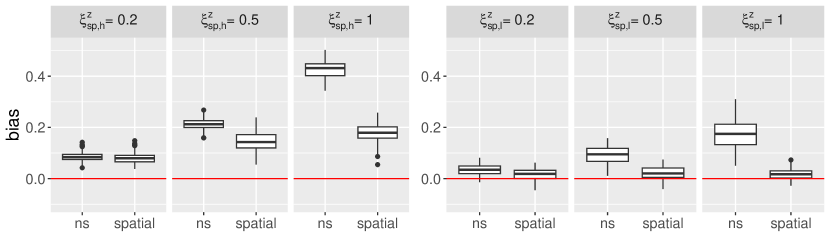
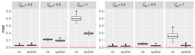
Figure 1: Bias (top) of $\widehat{\beta}$ and $\widehat{\beta}_{\mathrm{ns}}$ and MSE (bottom) of spatial and non-spatial (ns) models for high frequency (left) and low frequency (right) confounding. The true value is $\beta=0.5$. All other parameters remain constant.

4.2 Scenario 2: Confounding at Low Frequencies

We reconsider Scenario 1 but now swap high and low frequencies (i.e. confounding is now at low frequencies). We do not expect to see much bias in the spatial model because the contributions to the bias $\xi_{\mathrm{sp,l}}^{x}\xi_{\mathrm{sp,l}}^{z}$ are multiplied by weights $w_{i}$ that are low. Given this, we now consider $(\xi_{\mathrm{sp,l}}^{x},\xi_{\mathrm{sp,h}}^{x})=(1,1)$, $\xi_{\mathrm{sp,h}}^{z}=0$ and $\xi_{\mathrm{sp,l}}^{z}\in\{0.2,0.5,1\}$.

The results are shown in Figure 1 (top right). As expected, when confounding only happens at low frequencies, the bias is close to zero in the spatial model and remains close to zero as $\xi_{\mathrm{sp,l}}^{z}$ increases. In contrast, the non-spatial model has a positive and linearly increasing bias. Indeed, in the non-spatial case, as expected, the behaviour of the bias is the same for increasing $\xi_{\mathrm{sp,l}}^{z}$ and $\xi_{\mathrm{sp,h}}^{z}$ in both our high and low frequency scenarios.

Figure 1 (bottom right) shows the MSE of the fitted model compared to the true expectation of $\mathbf{y}$ in both the non-spatial and spatial models. The MSE is lower for the spatial model, which is expected since the non-spatial model is mis-specified.

4.3 Scenario 3: Confounding at High Frequencies, Low Correlation

In the previous scenario, we studied the effect of high and low frequency confounding on the bias of the spatial and non-spatial models. While results might hint at a better performance of the spatial model, this is not always the case. Indeed, by including high frequency confounded components and low frequency unconfounded components in $\mathbf{x}$, one can generate data where the correlation between $\mathbf{x}$ and $\mathbf{z}$ is overall low, but strong at high frequencies. This should lead to low bias in the non-spatial model but large bias in the spatial model.

Specifically, we consider $\xi_{\mathrm{sp,h}}^{x}\xi_{\mathrm{sp,h}}^{z}\neq 0$ and increase the amount of unconfounded spatial information in $\mathbf{x}$ when compared to Scenario 1 by increasing the coefficient $\xi_{\mathrm{sp,l}}^{x}$. The coefficient $\xi_{\mathrm{sp,l}}^{x}$ only contributes to the denominator of the bias as it relates to unconfounded frequencies. In the spatial model, this contribution is multiplied by relatively small weights $w_{i}$ as it corresponds to low frequency behaviour. In contrast, the weight is always 1 in the non-spatial model. Therefore, if we increase $\xi_{\mathrm{sp,l}}^{x}$ keeping everything else fixed, it will reduce the bias in both models, but have a much larger effect on the bias in the non-spatial model. Concretely, we consider $\xi_{\mathrm{sp,h}}^{x}=1$, $\xi_{\mathrm{sp,l}}^{z}=0$, $\xi_{\mathrm{sp,l}}^{x}\in\{1,20\}$ and $\xi_{\mathrm{sp,h}}^{z}\in\{0.2,0.5,1\}$. The case with $\xi_{\mathrm{sp,l}}^{x}=1$ corresponds to Scenario 1 and it is used for the sake of comparison.

The results in Figure 2 (right) confirm that by increasing $\xi_{\mathrm{sp,l}}^{x}$ we can reach scenarios where the non-spatial model has smaller bias than the spatial model. The MSE in Figure 2 (right) of the non-spatial model is always larger than the spatial model’s. Again, this is expected since the data is spatial. The results on the left match exactly those on the left of Figure 1 and are shown for comparison.

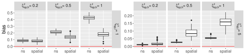
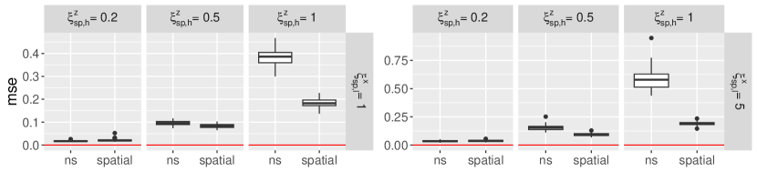
Figure 2: Bias of $\widehat{\beta}$ and $\widehat{\beta}_{\mathrm{ns}}$ (left) and MSE (right) of non-spatial (ns) and spatial models (right) for different combinations of $\xi_{\mathrm{sp,h}}^{z}$ and $\xi_{\mathrm{sp,l}}^{x}$. The true value is $\beta=0.5$. All other parameters remain constant.

4.4 Scenario 4: Dependence on Non-Spatial Information

Generally, spatial confounding is an issue when there is not enough non-spatial information in $\mathbf{x}$ or there are not sufficient unconfounded high frequencies in $\mathbf{x}$. Here we show the effect of non-spatial information on the bias in spatial and non-spatial models. Particularly, we consider the effects of increasing $\sigma_{x}$. This increase should correspond to increases in $\xi_{\mathrm{ns}}^{x}$ leading to drops in the bias in both spatial and non-spatial models. We consider $\sigma_{x}\in\{0.3,1,2,3\}$. Other parameters remain constant at $(\xi_{\mathrm{sp,l}}^{x},\xi_{\mathrm{sp,h}}^{x})=(1,1)$, $(\xi_{\mathrm{sp,l}}^{z},\xi_{\mathrm{sp,h}}^{z})=(0,0.5)$.

As shown in Figure 3 (top), the bias decreases for both the non-spatial and spatial model when $\sigma_{x}$ is increased. The MSE in Figure 3 (bottom) is always larger for the non-spatial model, as expected, as the data is spatial.

The relationship between the spatial and non-spatial bias is not always straightforward, as the the difference between the two is the weights $w_{i}$, which affect both the numerator and denominator. In Section 3.2, it is shown that the bias in the non-spatial model tends to be larger than that of the spatial model, but if the covariate has little non-spatial information and confounding takes place at high frequencies, then the bias in the spatial model may well exceed that of the non-spatial model. This behaviour can be observed in Figure 3 where the non-spatial bias is higher than the spatial, except in the case where $\sigma_{x}=0.3$, i.e. the case where $\mathbf{x}$ has the smallest amount of non-spatial information.

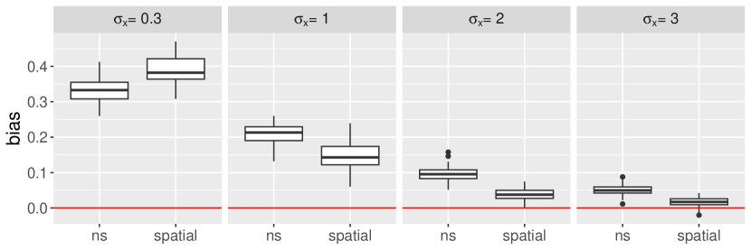
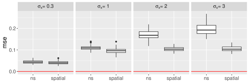
Figure 3: Bias of $\widehat{\beta}$ and $\widehat{\beta}_{\mathrm{ns}}$ (top) and MSE (bottom) of spatial and non-spatial models for different values of $\sigma_{x}$. The true value is $\beta=0.5$. All other parameters remain constant.

4.5 Scenario 5: Dependence on the Smoothing Parameter

As detailed in Section 3, when there is sufficient non-spatial information or unconfounded high frequency components in $\mathbf{x}$ and there are not many confounded unpenalised spatial components in $\mathbf{x}$, we expect the bias in the spatial model to be close to zero when $\lambda\rightarrow 0$, broadly increase as a function of $\lambda$ and to approach the size of the bias in the corresponding non-spatial model as $\lambda\rightarrow\infty$. However, the expression for the bias has a relatively complex dependency on $\lambda$, and as shown in Scenario 3, if we have confounding at high frequencies as well as unconfounded weakly penalised spatial frequencies, then the bias can also exceed that of the non-spatial model.

Here, we consider scenarios with confounding at high frequencies, unconfoundedness at low frequencies and with increasing amount of non-spatial information, where the latter is obtained by increasing the value of $\sigma_{x}$. For this, we use 10 basis functions to generate $\mathbf{z}_{\mathrm{sp,l}}$ and 800 basis functions for $\mathbf{z}_{\mathrm{sp,h}}$. Moreover, we consider $(\xi_{\mathrm{sp,l}}^{x},\xi_{\mathrm{sp,h}}^{x})=(1,1)$, $(\xi_{\mathrm{sp,l}}^{z},\xi_{\mathrm{sp,h}}^{z})=(0,0.5)$, $\sigma=1$, and fix $\lambda$ to different values. We let $\sigma_{x}\in\{0.3,1,2\}$. We now consider 20 replicates and show the results for the average spatial and non-spatial bias for those replicates and also use 800 basis functions in the data analysing model. These settings are chosen to broadcast a wide range of situations for the bias of the spatial model for increasing $\lambda$. While for lower values of $\sigma_{x}$ we might find situations where the bias of the spatial model crosses that of the non-spatial model and mostly remains at higher values, for higher values of $\sigma_{x}$ the spatial bias should mostly be below the bias of the non-spatial model. Unless there are many unpenalised spatial components in $\mathbf{x}$, we expect the spatial bias to eventually meet the non-spatial bias for large $\lambda$ in every case.

The results are shown in Figure 4. For $\sigma_{x}=0.3$, the bias of the spatial model, increases from 0, crosses that of the non-spatial model and mostly stays above it, until they meet again for large $\lambda$. As expected, increasing the non-spatial information in $\mathbf{x}$ decreases bias in general, and for $\sigma_{x}=1$, the bias of the spatial model is always lower than the one in the non-spatial model. The same is true for $\sigma_{x}=2$.

In Figure 4, we also show the median smoothing parameter estimated by GCV for each DGP, which has been used in the data analysing model in the previous simulation studies. We reach a bias of 0.4037, 0.1804 and 0.0362, respectively, from left to right. For the low non-spatial information scenario with $\sigma_{x}=0.3$, the GCV is beyond the steepest part of the curve, where the spatial bias changes a lot for small changes in $\hat{\lambda}$, and in a relatively flat area of the curve where the spatial bias exceeds the non-spatial. For higher non-spatial information, the estimate stays at the steep part of the curve, indicating that small changes in the estimated $\hat{\lambda}$ can lead to very strong differences in bias, although the bias remains below the one in the non-spatial model.

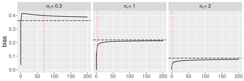
Figure 4: Bias of $\widehat{\beta}$ (solid black) and $\widehat{\beta}_{\mathrm{ns}}$ (dashed black) for increasing $\lambda$ and different $\sigma_{x}$. The true value is $\beta=0.5$. All other parameters remain constant. Magenta dashed line represents the median $\hat{\lambda}$ estimated by GCV. The bias associated with each $\hat{\lambda}$ is 0.4037, 0.1804 and 0.0362, from left to right.

5 Understanding Earlier Results on Spatial Confounding

The explicit analytical expressions in Propositions 3.1 and 3.5 and their corollaries provide an intuitive and quantifiable way of understanding spatial confounding in the general context of spatial mixed models. Our analysis in Sections 3 and 4 also shows why different choices of simulation set-ups and parameter ranges can easily lead to different conclusions. In this section, we use our results as a unified theoretical framework for understanding and generalising the main results on spatial confounding to date, and for clearing up some of the confusion that has surrounded research into this topic. Rather than an in-depth analysis of specific methods, this is intended as an overview that illustrates how our results can be applied in practice, not only for gaining intuition, but also for understanding how different aspects of the spatial confounding literature relate to each other.

One important assumption that is not usually highlighted in the literature is whether the covariate $\mathbf{x}$ has non-spatial information (i.e. whether $\boldsymbol{\xi}^{x}_{\mathrm{ns}}$ is non-zero). In most references, this assumption is only implicit and needs to be inferred from the set-up of a theoretical analysis or the way in which data are generated in a simulation. However, as was illustrated in Section 3 by the comparison to the non-spatial model and the dependence of the bias on the smoothing parameter $\lambda$, the bias may exhibit fundamentally different behaviour depending on whether or not this assumption holds. As we will see in Section 5.2, this assumption also has a direct impact on which methods are appropriate to use when estimating or adjusting for the bias. We note that since our expressions for the bias in Section 3 include $\boldsymbol{\xi}^{x}_{\mathrm{ns}}$, they can be used to consider both the case where $\boldsymbol{\xi}^{x}_{\mathrm{ns}}$ is non-zero and where it is not.

5.1 The Role of Spatial Scales

As the expressions in Section 3 involve the confounder $\mathbf{z}$ which, in practice, is unknown or unmeasured, we cannot simply compute the bias to assess the impact of confounding in a given situation. However, as we have seen, the expressions clarify which scenarios are more/less likely to lead to bias. Our conclusions are, in fact, in line with those of Paciorek, (2010) (which were also confirmed by Page et al., (2017)) who studied the case where the covariate is fully spatial (i.e. $\boldsymbol{\xi}^{x}_{\mathrm{ns}}=\boldsymbol{0}$) and pointed out how the size and occurrence of bias is related to the spatial scales (i.e. equivalent to the spatial frequencies) of both the covariate and the confounder. Thus, our expressions provide an explicit way of understanding these results in a more general framework, in particular, our derivations show that the conclusions still hold in the case where $\boldsymbol{\xi}^{x}_{\mathrm{ns}}$ is non-zero. That is, any confounded spatial frequency in $\mathbf{x}$ creates bias (unless the frequency is unsmoothed), but high frequency components create the largest bias, while confounding at low frequencies is less problematic. At the same time, any non-spatial information as well as any unconfounded frequency components in $\mathbf{x}$ reduce the size of the bias with higher reduction for higher frequencies.

In addition to this, we see that if the unmeasured spatial effect $\mathbf{z}$ has none of the spatial frequencies contained in the covariate (i.e. if there is no confounding) or if the confounded frequencies are unsmoothed, then the covariate effect estimate in the spatial model is unbiased. That is, in this scenario, the spatial model successfully adjusts for unmeasured spatial variation without causing unwanted bias.

While the work of Paciorek, (2010) is generally well-known, results on spatial scales seem to have created some confusion in the past, where there has been a tendency to worry more about confounding at low spatial frequencies despite this being the less problematic scenario. This is perhaps because low frequencies may be seen as more likely to be confounded in practice, with higher frequencies in $\mathbf{x}$ expected to capture the more characteristic behaviour specific to the covariate. Moreover, as seen from our comparison between the bias in the spatial model vs. that of the non-spatial model, low frequency confounding can also lead to large differences in the estimates in these two models. Historically, such differences were interpreted as a sign of confounding with the non-spatial estimate mistakenly assumed to be unbiased. In fact, our results confirm that bias in the spatial model is unlikely to be a problem when confounding is at low frequencies, as long as there is (sufficient) non-spatial information or unconfounded higher frequencies in the covariate.

5.2 Adjustment Methods

A number of recent results in the literature (Guan et al.,, 2023; Dupont et al.,, 2022; Thaden and Kneib,, 2018; Keller and Szpiro,, 2020) develop methods for estimating or reducing the bias in the spatial model (3) under various assumptions. Here we show how our simple formulation can be used to provide some intuition as to how these methods work, as well as clarifying the assumptions (whether explicitly stated or otherwise) that are utilised.

As discussed in Section 5.1, assumptions of spatial scales play a key role in determining the bias. Keller and Szpiro, (2020) suggest some approaches for bias adjustment based on spatial scale information, using Fourier, wavelet and thin plate regression spline methods to estimate the frequency components of the observed data. This type of analysis is useful for understanding the characteristic behaviour of the variables and, particularly, identifying whether $\mathbf{x}$ has non-spatial information, however, in general we cannot expect to estimate the bias based on the data alone. We will see below that if $\mathbf{x}$ has non-spatial information, then the non-spatial component can be used to identify the true covariate effect. But otherwise, the bias is directly related to the frequency components of $\mathbf{z}$ which are unknown and can only be identified under untestable assumptions.

Case 1: $\mathbf{x}$ has non-spatial information
Assume that the covariate $\mathbf{x}$ has non-spatial information, i.e. that $\boldsymbol{\xi}^{x}_{\mathrm{ns}}$ is non-zero. This means that, while the spatial locations at which the data are collected induce some spatial dependency structure in the covariate, there is some additional variation in the covariate data that cannot be explained by the spatial information alone.

Under this assumption, the model (3) is identifiable (i.e. the model matrix has full rank) and if there had been no smoothing (i.e. if $\lambda=0$), then the covariate effect estimate is the ordinary least squares estimate which, as long as the model is correctly specified, is unbiased. Smoothing is applied here in order to improve the fit of the model, i.e. to reflect the spatial covariance structure and avoid overfitting the spatial effect. This introduces bias in the estimates but reduces variance (the well-known bias-variance trade-off), and the optimal level of smoothing is usually chosen to minimise some measure of prediction error. However, while smoothing is only applied to the spatial part of the model, it also results in unwanted bias in the effect estimate of the covariate. If our only objective was to avoid this bias, then we could simply remove or reduce the level of smoothing in the model. This is explicitly illustrated in our results which show that whenever $\boldsymbol{\xi}^{x}_{\mathrm{ns}}$ is non-zero, then the bias becomes zero as $\lambda\rightarrow 0$. However, undersmoothing is, of course, undesirable from the point of view of model fit.

Spatial+ (Dupont et al.,, 2022) is an adjustment method for reducing or eliminating the bias in this case without adversely affecting the fit of the model. In spatial+ a spatial model with no covariates is firstly fitted to the covariate $\mathbf{x}$ in order to identify its spatial components. The residuals $\mathbf{r}^{x}$ in this initial regression are used as an estimate for the non-spatial part $\mathbf{x}_{\mathrm{ns}}=\mathbf{U}_{\mathrm{ns}}\boldsymbol{\xi}^{x}_{\mathrm{ns}}$ of $\mathbf{x}$. The covariate effect in the original spatial model is then estimated by fitting the model (3) but with $\mathbf{x}$ replaced by $\mathbf{r}^{x}$. Replacing $\mathbf{x}$ by $\mathbf{r}^{x}=\widehat{\mathbf{x}_{\mathrm{ns}}}$ in the expression for the bias in Proposition 3.1 shows why this can be expected to eliminate the bias (as $\langle\mathbf{x}_{\mathrm{ns}},\mathbf{z}\rangle_{\mathbf{\Sigma}^{-1}}=0$). The success of the method will depend on how well the initial regression approximates $\mathbf{x}_{\mathrm{ns}}$, in particular, the assumption is that this regression removes any confounded components in $\mathbf{x}$.

An alternative to spatial+ is the geoadditive structural equations model (gSEM) (Thaden and Kneib,, 2018). For this method, initial spatial regressions are used on both the covariate $\mathbf{x}$ and the response data $\mathbf{y}$ to estimate the non-spatial information, i.e. we obtain residuals $\mathbf{r}^{x}=\widehat{\mathbf{x}_{\mathrm{ns}}}$ and $\mathbf{r}^{y}=\widehat{\mathbf{y}_{\mathrm{ns}}}$. The covariate effect is then estimated as the effect of $\mathbf{r}^{x}$ on $\mathbf{r}^{y}$. The method is based on the structural equations framework from the causal inference literature which shows that the unbiased (or causal) effect of a covariate on a response variable can be obtained by removing the effect of confounders from both variables. In gSEM, the effect of spatial confounders is removed by removing all spatial information. Once again, the bias reduction will only be successful under the assumption that the initial regressions successfully remove all spatial confounders.

In summary, when $\boldsymbol{\xi}^{x}_{\mathrm{ns}}$ is non-zero, the spatial model has the information necessary to distinguish the effect of $\mathbf{x}$ from that of $\mathbf{z}$, however, bias in the covariate effect estimate arises as a result of the distortion caused by spatial smoothing. Spatial+ and gSEM both use estimates of the unconfounded component $\mathbf{x}_{\mathrm{ns}}=\mathbf{U}_{\mathrm{ns}}\boldsymbol{\xi}^{x}_{\mathrm{ns}}$ to eliminate this bias.

Case 2: $\mathbf{x}$ is fully spatial
Assume that $\mathbf{x}$ has no non-spatial components (i.e. that $\boldsymbol{\xi}^{x}_{\mathrm{ns}}=\mathbf{0}$). This could, for example, be the case if $\mathbf{x}$ is assumed to be generated from a smooth spatial process. Another way that this situation could arise is if the spatial effect in model (3) has the same dimension as the sample size, i.e. $n=p$. An example of this is a regional ICAR model with only one data measurement per region.

In this case the spatial model is unidentifiable; the covariate vector $\mathbf{x}$ is contained in the space spanned by the spatial basis vectors and, therefore, the model matrix is rank deficient. This means that the effect of $\mathbf{x}$ can be modelled either as part of the fixed effect term or as part of the spatial effect, and there are infinitely many possibilities for splitting the effect between these two terms. Here, the smoothing penalty is not only a mechanism for avoiding overfitting, but also acts as a regulariser, i.e. it enables the model to be fit, choosing a particular split of the covariate effect which may or may not correspond to the truth. (Note that the model cannot be fitted without smoothing, i.e. if $\lambda=0$). Our expression for the bias still holds and shows what happens in different scenarios with the same conclusions as before about which situations cause most bias. But unlike Case 1 where $\mathbf{x}$ has non-spatial information (which is always unconfounded), we have no information of the confounding scenario and therefore the behaviour will generally be harder to predict. In particular, we no longer have the result that the bias approaches zero as $\lambda\rightarrow 0$ and, contrary to intuition, the bias could even increase as smoothing is reduced.

Note that, although the previously mentioned work by Keller and Szpiro, (2020) could be used to analyse the scale behaviour in the observed variables $\mathbf{y}$ and $\mathbf{x}$, the bias cannot be estimated without further (untestable) assumptions for identifiability. More specifically, the spatial frequency components of the response variable $\mathbf{y}$ will be a combination of the spatial frequencies of the covariate $\mathbf{x}$ and those of the unknown variable $\mathbf{z}$. Estimating the spatial frequency components of both $\mathbf{y}$ and $\mathbf{x}$, we can therefore determine some of the frequency content of $\mathbf{z}$, namely, the frequencies that are present in $\mathbf{y}$ but not in $\mathbf{x}$. However, as we can see from our expressions, these frequencies provide no information about the bias in the covariate effect as they are independent of $\mathbf{x}$. The remaining frequencies (that are present in both $\mathbf{y}$ and $\mathbf{x}$) could all potentially be present in $\mathbf{z}$ and are therefore unidentifiable.

Guan et al., (2023) outlines two approaches for obtaining identifiability in the model when $\mathbf{x}$ and $\mathbf{z}$ are realisations of two stationary Gaussian spatial processes: 1) unconfoundedness at high frequencies and 2) parsimonious cross-covariance, where a Fourier transform rather than the eigendecomposition is used to describe spatial frequencies. The latter approach is the assumption that the correlation between the covariate and the confounder is constant across spatial frequencies, which does not in itself lead to identifiability, but may simplify computations. Here, we focus on assumption 1) and use the expression in Corollary 3.2 to show that the ideas extend to our more general framework.

Unconfoundedness at higher frequencies is, in our framework, the assumption that $\xi^{z}_{\mathrm{sp},i}=0$ for eigenvectors with frequencies above a certain threshold. If this is the case, then the frequency components of $\mathbf{x}$ above this threshold can be used to obtain identifiability. As noted in Guan et al., (2023), this assumption seems natural as the highest frequency spatial variation in the covariate is more likely to be characteristic to the covariate and therefore not confounded with other spatial variables. Guan et al., (2023) suggest using a spline-based method in the Fourier frequency domain to obtain an estimate of the appropriate threshold. Based on this they then estimate the confounder $\mathbf{z}$.

Under this assumption, we could also use spatial+, described in the Case 1 scenario above, to eliminate the bias. Although $\mathbf{x}$ no longer has a non-spatial component, as we have seen, unconfounded high frequencies have a similar effect on the bias as non-spatial information. The residuals $\mathbf{r}^{x}$ in the first stage regression of spatial+ will be dominated by the highest frequency components in $\mathbf{x}$. Therefore, it seems reasonable to use $\mathbf{r}^{x}$ as an estimate $\widehat{\mathbf{x}_{\mathrm{uc}}}$ of an unconfounded component of $\mathbf{x}$. This is similar to Guan et al., (2023) but instead of using a spline to identify a threshold frequency, we use the spatial model itself to estimate the least spatially smooth behaviour in $\mathbf{x}$ and assume that this is unconfounded. Thus, by replacing $\mathbf{x}$ by $\mathbf{r}^{x}$ in model (3) we would once again expect to eliminate the bias (as $\langle\mathbf{x}_{\mathrm{uc}},\mathbf{z}\rangle_{\mathbf{\Sigma}^{-1}}=0$). Of course, this approach would only be appropriate if we believe that the residuals $\mathbf{r}^{x}$ are actually a part of $\mathbf{x}$ and not simply measurement noise, as otherwise $\mathbf{r}^{x}$ would contain no information about the covariate effect. Note, however, that any estimate $\widehat{\mathbf{x}_{\mathrm{uc}}}$ could be used in the second stage regression of spatial+. In particular, an alternative to doing the first stage regression is to simply assume that the frequencies in $\mathbf{x}$ above a certain threshold are an unconfounded part of $\mathbf{x}$ and use this component as $\widehat{\mathbf{x}_{\mathrm{uc}}}$ instead of $\mathbf{r}^{x}$.

The assumption of unconfoundedness could also be made more explicit by removing the highest frequencies from the spatial part of the model matrix of model (3), i.e. we essentially define these frequencies of $\mathbf{x}$ to be “non-spatial”. Then we obtain an identifiable model matrix and we are back in the Case 1 scenario above, where adjustment methods such as spatial+ and gSEM (where all spatial regressions also have the highest frequencies removed) can once again be used to adjust for bias. In fact, we note that, in principle, any unconfounded frequencies in the covariate (whether they are the highest frequencies or not) can be used to identify the covariate effect. Indeed, setting particular frequencies to $0$ in the spatial effect is a special case of imposing a linear constraint on the parameters in model (3) of the form

$$\mathbf{C}\boldsymbol{\beta}_{\mathrm{sp}}=\mathbf{0}$$ (6)

for some $n\times p$ matrix $\mathbf{C}$. This is a standard method for obtaining identifiablity in linear models e.g. when working with factor variables. So if we believe particular frequencies or linear combinations of frequencies to be unconfounded, these could be removed from the spatial effect and treated as “non-spatial”.

Finally, note that none of the above approaches can be used if there are no unconfounded components in $\mathbf{x}$. In this case, $\mathbf{z}=a\mathbf{x}$ for some $a\in\mathbb{R}$ (when we ignore any components of $\mathbf{z}$ that are independent of $\mathbf{x}$ and therefore do not affect the bias). Thus, the expression for the bias in Proposition 3.1 becomes simply $a$. The bias is independent of smoothing and is the same as the bias in the non-spatial model. What this reflects is that, when $\mathbf{x}$ is fully spatial and the confounding has the exact same spatial variation as $\mathbf{x}$, then linear projection methods such as regression cannot be used to distinguish the effect of $\mathbf{x}$ from the confounder; the only way to disentangle them is by making a direct assumption about $a$, i.e. the size of the bias.

5.3 Restricted Spatial Regression (RSR)

In this section we consider briefly the adjustment method of RSR introduced in Reich et al., (2006). For many years, this method was the go-to method for dealing with spatial confounding, and research into the topic was dominated by developments within the RSR framework. More recently, however, the method has come under some criticism (Khan and Calder,, 2022; Zimmerman and Ver Hoef,, 2022) and it is no longer seen as an appropriate approach for bias adjustment in the context of spatial confounding. Our results confirm this. Indeed, our expressions for the bias in the spatial model provide a simple and intuitive way to see that RSR does not work as intended.

RSR is designed to recover the effect estimate in the non-spatial model (4) by restricting the spatial effect in model (3) to the orthogonal complement of the covariate. This restriction ensures that the covariate effect is estimated independently from the spatial effects, and the intention is to thereby avoid interference from potential confounders. Note that RSR is a special (extreme) case of the method described in Section 5.2 (Case 2) of removing spatial frequencies from the spatial effect, namely, where all the frequencies present in the covariate are removed (or, equivalently, where the matrix $\mathbf{C}$ in (6) is chosen so that the spatial effect is projected onto the orthogonal complement of $\mathbf{x}$).

The method has been advocated, particularly, for estimating the unconditional effect of $\mathbf{x}$ on the response variable when the spatial effect is believed to be a random process representing “spatially structured noise” independent of $\mathbf{x}$. The RSR adjustment is proposed because, while any single realisation $\mathbf{z}$ of the process may have components which make the correlation between $\mathbf{x}$ and $\mathbf{z}$ non-zero (and therefore induce bias in the spatial model), when averaged over all realisations, the correlation should be zero. In the context of spatial confounding, however, a random variable (representing, for example, a missing covariate) would only be considered a confounder if its correlation with $\mathbf{x}$ is non-zero (i.e. if some components $\xi_{\mathrm{sp},i}^{x}\xi_{\mathrm{sp},i}^{z}$ of the quantity $\langle\mathbf{x},\mathbf{z}\rangle$ are non-zero when averaged over all realisations $\mathbf{z}$). Thus, the assumption of independence is equivalent to the assumption that there are no spatial confounders. Our analysis shows that, under this assumption, the expected bias in the covariate effect estimate of the spatial model (3) is indeed $0$. Therefore, restricting the spatial effect in this way is either unnecessary (if the assumption of independence holds) or the restriction actually introduces bias (if the assumption doesn’t hold).

In summary, if the spatial effect is believed to be “spatially structured noise” independent of $\mathbf{x}$, then the unadjusted spatial model is the more appropriate model to use. If, conversely, the spatial effect is expected to include a confounder, then RSR would also be inappropriate, as the method is equivalent to removing from the spatial effect all frequencies that could potentially be confounded.

6 Conclusion

In this paper, the central result is the intuitive analytical expression for the bias arising from spatial confounding provided in Proposition 3.1 as well as the more detailed version in Corollary 3.2. From these expressions it follows that the bias is a direct result of spatial smoothing in the analysing model which exists even if the model is correctly specified. We can also explicitly see what the bias depends on, namely, the confounding scenario (determined by the coefficients $\boldsymbol{\xi}^{x}$ and $\boldsymbol{\xi}^{z}$), the chosen spatial covariance structure (which determines the weights $w_{i}$) and the parameters in the model ($\sigma^{2}$ and $\lambda$).

Analysing these expressions we gain a full picture of the behaviour of the bias. In particular, we can identify which situations are more/less likely to lead to bias. We see that confounded components in $\mathbf{x}$ add to the bias while unconfounded components in $\mathbf{x}$ reduce the size of the bias, but as different components have different weights (determined by the spatial covariance structure of the model) they affect the bias differently. Thus, high spatial frequency components of $\mathbf{x}$ (which typically have larger weights) tend to have a larger effect on the bias while low frequency components have smaller impact. We also see that non-spatial information in the covariate reduces the size of the bias, while components of the true spatial effect $\mathbf{z}$ that are independent of $\mathbf{x}$ have no effect on the bias (except an indirect effect through the estimates of $\sigma^{2}$ and $\lambda$). Finally, we see that the size of the bias grows in line with the size of the confounder. We conclude that, spatial confounding is unlikely to be an issue if confounding is only at low frequencies or the covariate has a lot of non-spatial or unconfounded information. However, when there are confounders at high frequencies and the covariate has little non-spatial or unconfounded high frequency information, then bias could become significant. In fact, as the size of the confounder is unknown, the bias could be arbitrarily large.

The expressions for the bias also show exactly how different features of the model and the data generation process affect the size of the bias and how the bias compares to that of the non-spatial model. While the expressions are fairly simple, the dependence on specific components can be quite complicated. Having explicit expressions for the bias is therefore particularly helpful for understanding subtleties and avoiding confusion. For example, although the bias is induced by smoothing and can broadly be expected to increase as a function of the smoothing parameter $\lambda$, there are confounding scenarios and areas within the parameter space where this function is decreasing. Similarly, while the bias in the spatial model is generally smaller than that of the non-spatial model, there are situations in which it is the other way around. Of course, as our simulations also show, irrespective of this comparison, the non-spatial model is inappropriate to use as it is mis-specified and therefore leads to poorer fit.

Our results can also be used as a broad framework for understanding and generalising previous research into spatial confounding. This includes the results on the importance of spatial scales (Paciorek,, 2010; Page et al.,, 2017), the conclusions of which become very clear using the expression for the bias in Corollary 3.2. We also discuss how different suggested methods for alleviating spatial confounding fit into our framework and show that such methods fundamentally rely on untestable assumptions about the confounding scenario. As different methods may well lead to different results, it is important to be aware of the assumptions used in each case. Here, our derivations can once again be used to understand, in a simple and intuitive way, which methods are appropriate to use under different scenarios. In particular, we see how the choice of method could depend on whether the covariate is assumed to have non-spatial information.

Since spatial regression models can also be considered as mixed models with spatially correlated random effects, our framework can also be carried forward to other random effects models, e.g. for grouped and longitudinal data. This might allow us to establish links to endogeneity considerations for panel data in econometrics, but also points towards potential confounding effects in other forms of regression analyses. Similarly, extending our considerations to spatio-temporal confounding should provide us with important insights on how spatial and/or temporal structures lead to biased estimates.

Finally, it is important to note that our, as well as most other work on spatial confounding, focuses on quantifying the bias of fixed effects in spatial regression. To put this bias into perspective and to thoroughly conduct statistical inference, more investigations on associated uncertainty will be an important direction for future research.

Appendix A Appendix

A.1 Proof of Lemma 2.1

Let $\mathbf{M}=\sigma^{-2}(\mathbf{I}-\mathbf{A})$. Then

$$\mathbf{\Sigma}\mathbf{M} = (\sigma^{2}\mathbf{I}+\lambda^{-1}\mathbf{B}_{\mathrm{sp}}\mathbf{S}^{-}\mathbf{B}_{\mathrm{sp}}^{T})\left(\sigma^{-2}\mathbf{I}-\sigma^{-4}\mathbf{B}_{\mathrm{sp}}(\sigma^{-2}\mathbf{B}_{\mathrm{sp}}^{T}\mathbf{B}_{\mathrm{sp}}+\lambda\mathbf{S})^{-1}\mathbf{B}_{\mathrm{sp}}^{T}\right)$$

$$= \mathbf{I}+\sigma^{-2}\lambda^{-1}\mathbf{B}_{\mathrm{sp}}\mathbf{S}^{-}\mathbf{B}_{\mathrm{sp}}^{T}-\sigma^{-2}\mathbf{B}_{\mathrm{sp}}(\sigma^{-2}\mathbf{B}_{\mathrm{sp}}^{T}\mathbf{B}_{\mathrm{sp}}+\lambda\mathbf{S})^{-1}\mathbf{B}_{\mathrm{sp}}^{T}$$

$$-\sigma^{-4}\lambda^{-1}\mathbf{B}_{\mathrm{sp}}\mathbf{S}^{-}\mathbf{B}_{\mathrm{sp}}^{T}\mathbf{B}_{\mathrm{sp}}(\sigma^{-2}\mathbf{B}_{\mathrm{sp}}^{T}\mathbf{B}_{\mathrm{sp}}+\lambda\mathbf{S})^{-1}\mathbf{B}_{\mathrm{sp}}^{T}$$

$$= \mathbf{I}+\sigma^{-2}\lambda^{-1}\mathbf{B}_{\mathrm{sp}}\mathbf{S}^{-}\left(\mathbf{I}-(\lambda\mathbf{S}+\sigma^{-2}\mathbf{B}_{\mathrm{sp}}^{T}\mathbf{B}_{\mathrm{sp}})(\sigma^{-2}\mathbf{B}_{\mathrm{sp}}^{T}\mathbf{B}_{\mathrm{sp}}+\lambda\mathbf{S})^{-1}\right)\mathbf{B}_{\mathrm{sp}}^{T}$$

$$= \mathbf{I}.$$

Hence $\mathbf{\Sigma}^{-1}=\mathbf{M}$. ∎

A.2 Proof of Lemma 2.2

As $\mathbf{S}$ is symmetric, $\mathbf{A}$ is also symmetric. Without loss of generality we can assume that the spatial basis $\mathbf{B}_{\mathrm{sp}}$ is orthonormal so that $\mathbf{B}_{\mathrm{sp}}^{T}\mathbf{B}_{\mathrm{sp}}=\mathbf{I}$ and

$$\mathbf{A}=\sigma^{-2}\mathbf{B}_{\mathrm{sp}}(\sigma^{-2}\mathbf{I}+\lambda\mathbf{S})^{-1}\mathbf{B}_{\mathrm{sp}}^{T}.$$

Clearly anything in the null space of $\mathbf{A}$ (i.e. the orthogonal complement of the column space of $\mathbf{B}_{\mathrm{sp}}$, which is the “non-spatial” part of $\mathbb{R}^{n}$) is an eigenvector with eigenvalue $0$.

Suppose $\mathbf{v}\in\mathbb{R}^{p}$ is an eigenvector of $\mathbf{S}$ with eigenvalue $\alpha_{i}$. Let $\mathbf{v}^{\prime}=\mathbf{B}_{\mathrm{sp}}\mathbf{v}$. Then $\mathbf{v}^{\prime}\in\mathbb{R}^{n}$ and

$$\mathbf{A}\mathbf{v}^{\prime} = \sigma^{-2}\mathbf{B}_{\mathrm{sp}}(\sigma^{-2}\mathbf{I}+\lambda\mathbf{S})^{-1}\mathbf{B}_{\mathrm{sp}}^{T}\mathbf{B}_{\mathrm{sp}}\mathbf{v}$$

$$= \sigma^{-2}\mathbf{B}_{\mathrm{sp}}(\sigma^{-2}\mathbf{I}+\lambda\mathbf{S})^{-1}\mathbf{v}$$

$$= \sigma^{-2}\mathbf{B}_{\mathrm{sp}}(\sigma^{-2}+\lambda\alpha_{i})^{-1}\mathbf{v}$$

$$= \tfrac{\sigma^{-2}}{\sigma^{-2}+\lambda\alpha_{i}}\mathbf{v}^{\prime}.$$

Since all eigenvalues are non-negative, $\mathbf{A}$ is positive semi-definite. ∎

A.3 Proof of Lemma 2.3

By Lemma 2.1 we have that $\mathbf{\Sigma}^{-1}=\sigma^{-2}(\mathbf{I}-\mathbf{A})$ so the eigenvalues of $\mathbf{\Sigma}^{-1}$ are all of the form $\sigma^{-2}(1-\alpha)$ where $\alpha$ is an eigenvalue of $\mathbf{A}$. Lemma 2.2 gives us the eigenvalues of $\mathbf{A}$. The eigenvalue $\alpha=0$ (corresponding to the eigenvectors spanning the non-spatial part of $\mathbb{R}^{n}$) leads to the eigenvalue $\sigma^{-2}$ for $\mathbf{\Sigma}^{-1}$ and the remaining eigenvalues of $\mathbf{\Sigma}^{-1}$ are given by

$$\sigma^{-2}(1-\tfrac{\sigma^{-2}}{\sigma^{-2}+\lambda\alpha_{i}})=\tfrac{\sigma^{-2}\lambda\alpha_{i}}{\sigma^{-2}+\lambda\alpha_{i}},\quad\textrm{for }i=1,\ldots,p.$$

∎

A.4 Proof of Proposition 3.1

Since under the data generating model (2) $\operatorname{E}(\mathbf{y})=\beta\mathbf{x}+\mathbf{z}$, we have that

$$\operatorname{E}(\widehat{\beta}) = (\mathbf{x}^{T}\mathbf{\Sigma}^{-1}\mathbf{x})^{-1}\mathbf{x}^{T}\mathbf{\Sigma}^{-1}\operatorname{E}(\mathbf{y})$$

$$= (\mathbf{x}^{T}\mathbf{\Sigma}^{-1}\mathbf{x})^{-1}\mathbf{x}^{T}\mathbf{\Sigma}^{-1}(\beta\mathbf{x}+\mathbf{z})$$

$$= \beta+(\mathbf{x}^{T}\mathbf{\Sigma}^{-1}\mathbf{x})^{-1}\mathbf{x}^{T}\mathbf{\Sigma}^{-1}\mathbf{z}$$

$$= \beta+\frac{\langle\mathbf{x},\mathbf{z}\rangle_{\mathbf{\Sigma}^{-1}}}{\langle\mathbf{x},\mathbf{x}\rangle_{\mathbf{\Sigma}^{-1}}}.$$

∎

A.5 Proof of Corollary 3.2

The numerator of the bias in $\widehat{\beta}$ is given by

$$\langle\mathbf{x},\mathbf{z}\rangle_{\mathbf{\Sigma}^{-1}} = \mathbf{x}^{T}\mathbf{\Sigma}^{-1}\mathbf{z}$$

$$= \boldsymbol{\xi}^{xT}\mathbf{U}^{T}\mathbf{\Sigma}^{-1}\mathbf{U}\boldsymbol{\xi}^{z}$$

$$= \sigma^{-2}\boldsymbol{\xi}^{xT}_{\mathrm{ns}}\boldsymbol{\xi}^{z}_{\mathrm{ns}}+\sigma^{-2}\boldsymbol{\xi}^{xT}_{\mathrm{sp}}\begin{bmatrix}w_{1}&&\\ &\ddots&\\ &&w_{p}\end{bmatrix}\boldsymbol{\xi}^{z}_{\mathrm{sp}}$$

$$= \sigma^{-2}\boldsymbol{\xi}^{xT}_{\mathrm{sp}}\begin{bmatrix}w_{1}&&\\ &\ddots&\\ &&w_{p}\end{bmatrix}\boldsymbol{\xi}^{z}_{\mathrm{sp}}$$

$$= \sigma^{-2}\sum_{i=1}^{p}\xi_{\mathrm{sp},i}^{x}\xi_{\mathrm{sp},i}^{z}w_{i}.$$

Similarly, the denominator of the bias is given by

$$\langle\mathbf{x},\mathbf{x}\rangle_{\mathbf{\Sigma}^{-1}} = \sigma^{-2}\boldsymbol{\xi}^{xT}_{\mathrm{ns}}\boldsymbol{\xi}^{x}_{\mathrm{ns}}+\sigma^{-2}\boldsymbol{\xi}^{xT}_{\mathrm{sp}}\begin{bmatrix}w_{1}&&\\ &\ddots&\\ &&w_{p}\end{bmatrix}\boldsymbol{\xi}^{x}_{\mathrm{sp}}$$

$$= \sigma^{-2}\sum_{i=1}^{n-p}(\xi_{\mathrm{ns},i}^{x})^{2}+\sigma^{-2}\sum_{i=1}^{p}(\xi_{\mathrm{sp},i}^{x})^{2}w_{i}$$

∎

A.6 Comparison to the Non-Spatial Model

Using the expressions in Corollaries 3.2 and 3.3, we compute the difference between the bias $\mathrm{Bias}_{\mathrm{ns}}=\operatorname{E}(\widehat{\beta}_{\mathrm{ns}})-\beta$ in the non-spatial model (4) and the bias $\mathrm{Bias}=\operatorname{E}(\widehat{\beta})-\beta$ in the spatial model (3). As we are mainly interested in comparing the size of the bias, for simplicity assume that all $\xi_{\mathrm{sp},i}^{x}\xi_{\mathrm{sp},i}^{z}$ are positive. To simplify notation, let

$$C_{\mathrm{ns}}=\sum_{i=1}^{n-p}(\xi_{\mathrm{ns},i}^{x})^{2}\geq 0.$$

Then,

$$\mathrm{Bias}_{\mathrm{ns}}-\mathrm{Bias} = \frac{\sum_{i=1}^{p}\xi_{\mathrm{sp},i}^{x}\xi_{\mathrm{sp},i}^{z}}{C_{\mathrm{ns}}+\sum_{i=1}^{p}(\xi_{\mathrm{sp},i}^{x})^{2}}-\frac{\sum_{i=1}^{p}\xi_{\mathrm{sp},i}^{x}\xi_{\mathrm{sp},i}^{z}w_{i}}{C_{\mathrm{ns}}+\sum_{i=1}^{p}(\xi_{\mathrm{sp},i}^{x})^{2}w_{i}}$$

$$= \frac{\left(\sum_{i=1}^{p}\xi_{\mathrm{sp},i}^{x}\xi_{\mathrm{sp},i}^{z}\right)\left(C_{\mathrm{ns}}+\sum_{i=1}^{p}(\xi_{\mathrm{sp},i}^{x})^{2}w_{i}\right)}{\left(C_{\mathrm{ns}}+\sum_{i=1}^{p}(\xi_{\mathrm{sp},i}^{x})^{2}\right)\left(C_{\mathrm{ns}}+\sum_{i=1}^{p}(\xi_{\mathrm{sp},i}^{x})^{2}w_{i}\right)}$$

$$-\frac{\left(\sum_{i=1}^{p}\xi_{\mathrm{sp},i}^{x}\xi_{\mathrm{sp},i}^{z}w_{i}\right)\left(C_{\mathrm{ns}}+\sum_{i=1}^{p}(\xi_{\mathrm{sp},i}^{x})^{2}\right)}{\left(C_{\mathrm{ns}}+\sum_{i=1}^{p}(\xi_{\mathrm{sp},i}^{x})^{2}\right)\left(C_{\mathrm{ns}}+\sum_{i=1}^{p}(\xi_{\mathrm{sp},i}^{x})^{2}w_{i}\right)}.$$

The denominator of this expression is positive and the numerator can be written as

$$C_{\mathrm{ns}}\sum_{i=1}^{p}\xi_{\mathrm{sp},i}^{x}\xi_{\mathrm{sp},i}^{z}(1-w_{i})+\sum_{i,j}\xi_{\mathrm{sp},i}^{x}\xi_{\mathrm{sp},i}^{z}(\xi_{\mathrm{sp},j}^{x})^{2}(w_{j}-w_{i}).$$

Recall that $0\leq w_{1}\leq\cdots\leq w_{p}<1$ and note that $\xi_{\mathrm{sp},i}^{x}\xi_{\mathrm{sp},i}^{z}$ is non-zero exactly when frequency $i$ is confounded. Therefore, the first term in the numerator is strictly positive whenever there is confounding and $\mathbf{x}$ has non-spatial information, and is larger when confounded frequencies in $\mathbf{x}$ have low weights (i.e. are the low frequencies). The second term can be written as

$$\sum_{i<j}(\xi_{\mathrm{sp},i}^{x}\xi_{\mathrm{sp},i}^{z}(\xi_{\mathrm{sp},j}^{x})^{2}-\xi_{\mathrm{sp},j}^{x}\xi_{\mathrm{sp},j}^{z}(\xi_{\mathrm{sp},i}^{x})^{2})(w_{j}-w_{i}).$$

Since $w_{j}-w_{i}\geq 0$ for $i<j$, this shows that confounding at low frequencies ($\xi_{\mathrm{sp},i}^{x}\xi_{\mathrm{sp},i}^{z}\neq 0$) contribute positively to the sum, whereas confounding at high frequencies ($\xi_{\mathrm{sp},j}^{x}\xi_{\mathrm{sp},j}^{z}\neq 0$) contribute negatively. Conversely, unconfounded high frequencies ($\xi_{\mathrm{sp},j}^{x}\neq 0$, $\xi_{\mathrm{sp},j}^{z}=0$) contribute positively, while unconfounded low frequencies ($\xi_{\mathrm{sp},i}^{x}\neq 0$, $\xi_{\mathrm{sp},i}^{z}=0$) contribute negatively. Note that for a fixed unconfounded high frequency $j$ the contribution is given by

$$(\xi_{\mathrm{sp},j}^{x})^{2}\sum_{i=1}^{j-1}\xi_{\mathrm{sp},i}^{x}\xi_{\mathrm{sp},i}^{z}(w_{j}-w_{i})$$

with weight $w_{j}$ close to $1$. This shows that unconfounded high frequencies enter the expression in a similar way to non-spatial information.

Therefore, when $\mathbf{x}$ has sufficient non-spatial information or unconfounded high frequencies, then we can generally expect the bias of the non-spatial model to be higher than that of the spatial model, with the difference between the biases larger when there is a lot of confounding at low frequencies. However, the relationship between the two biases is subtle and, when confounding is at high frequencies, the bias in the spatial model could well exceed that of the non-spatial model.

A.7 Dependence on the Smoothing Parameter

We consider here how the expression for the bias given in Corollary 3.2 depends on the overall level of smoothing controlled by the smoothing parameter $\lambda>0$. For each $i=1,\ldots,p$, consider the i’th weight (5) as a function of $\lambda$:

$$w_{i}(\lambda)=\tfrac{\lambda\alpha_{i}}{\sigma^{-2}+\lambda\alpha_{i}}.$$

We see that $\lim_{\lambda\rightarrow 0}w_{i}(\lambda)=0$ and (unless $\alpha_{i}=0$ in which case $w_{i}(\lambda)\equiv 0$ is constant) $\lim_{\lambda\rightarrow\infty}w_{i}(\lambda)=1$. We also have that

$$w_{i}^{\prime}(\lambda)=\tfrac{\alpha_{i}\sigma^{-2}}{(\sigma^{-2}+\lambda\alpha_{i})^{2}}\geq 0.$$

Hence, the weights are either constant (and equal to 0) or increasing between 0 and 1.

Let

$$f(\lambda)=\frac{\sum_{i=1}^{p}\xi_{\mathrm{sp},i}^{x}\xi_{\mathrm{sp},i}^{z}w_{i}(\lambda)}{\sum_{i=1}^{n-p}(\xi_{\mathrm{ns},i}^{x})^{2}+\sum_{i=1}^{p}(\xi_{\mathrm{sp},i}^{x})^{2}w_{i}(\lambda)}$$

denote the bias in the spatial model for a given $\mathbf{x}$ and $\mathbf{z}$ as a function of $\lambda$. We then have that

$$f^{\prime}(\lambda) = \frac{\left(\sum_{i=1}^{p}\xi_{\mathrm{sp},i}^{x}\xi_{\mathrm{sp},i}^{z}w_{i}^{\prime}(\lambda)\right)\left(\sum_{i=1}^{n-p}(\xi_{\mathrm{ns},i}^{x})^{2}+\sum_{i=1}^{p}(\xi_{\mathrm{sp},i}^{x})^{2}w_{i}(\lambda)\right)}{\left(\sum_{i=1}^{n-p}(\xi_{\mathrm{ns},i}^{x})^{2}+\sum_{i=1}^{p}(\xi_{\mathrm{sp},i}^{x})^{2}w_{i}(\lambda)\right)^{2}}$$

$$\qquad-\frac{\left(\sum_{i=1}^{p}(\xi_{\mathrm{sp},i}^{x})^{2}w_{i}^{\prime}(\lambda)\right)\left(\sum_{i=1}^{p}\xi_{\mathrm{sp},i}^{x}\xi_{\mathrm{sp},i}^{z}w_{i}(\lambda)\right)}{\left(\sum_{i=1}^{n-p}(\xi_{\mathrm{ns},i}^{x})^{2}+\sum_{i=1}^{p}(\xi_{\mathrm{sp},i}^{x})^{2}w_{i}(\lambda)\right)^{2}}.$$

So the denominator of $f^{\prime}(\lambda)$ is positive and the numerator is given by

$$\sum_{i,k}\xi_{\mathrm{sp},i}^{x}\xi_{\mathrm{sp},i}^{z}w_{i}^{\prime}(\lambda)(\xi_{\mathrm{ns},k}^{x})^{2}+\sum_{i,j}\xi_{\mathrm{sp},i}^{x}\xi_{\mathrm{sp},i}^{z}(\xi_{\mathrm{sp},j}^{x})^{2}(w_{i}^{\prime}(\lambda)w_{j}(\lambda)-w_{j}^{\prime}(\lambda)w_{i}(\lambda)).$$

To consider the behaviour of the size of the bias, for simplicity assume that all $\xi_{\mathrm{sp},i}^{x}\xi_{\mathrm{sp},i}^{z}$ are positive. Then the first term in the numerator of $f^{\prime}(\lambda)$ is positive. Note that this term is non-zero if and only if $\mathbf{x}$ has non-spatial information. For the second term, we see that

$$w_{i}^{\prime}(\lambda)w_{j}(\lambda)-w_{j}^{\prime}(\lambda)w_{i}(\lambda) = \tfrac{\alpha_{i}\sigma^{-2}}{(\sigma^{-2}+\lambda\alpha_{i})^{2}}\tfrac{\lambda\alpha_{j}}{\sigma^{-2}+\lambda\alpha_{j}}+\tfrac{\alpha_{j}\sigma^{-2}}{(\sigma^{-2}+\lambda\alpha_{j})^{2}}\tfrac{\lambda\alpha_{i}}{\sigma^{-2}+\lambda\alpha_{i}}$$

$$= \tfrac{\lambda\alpha_{i}\alpha_{j}\sigma^{-2}}{(\sigma^{-2}+\lambda\alpha_{i})(\sigma^{-2}+\lambda\alpha_{j})}\left(\tfrac{1}{\sigma^{-2}+\lambda\alpha_{i}}-\tfrac{1}{\sigma^{-2}+\lambda\alpha_{j}}\right)$$

$$= \tfrac{\lambda^{2}\alpha_{i}\alpha_{j}\sigma^{-2}}{(\sigma^{-2}+\lambda\alpha_{i})^{2}(\sigma^{-2}+\lambda\alpha_{j})^{2}}(\alpha_{j}-\alpha_{i}).$$

So the second term of the numerator can be written as

$$\sum_{i,j}\xi_{\mathrm{sp},i}^{x}\xi_{\mathrm{sp},i}^{z}(\xi_{\mathrm{sp},j}^{x})^{2}c_{ij}(\lambda)(\alpha_{j}-\alpha_{i})$$

$$\quad=\sum_{i<j}\left(\xi_{\mathrm{sp},i}^{x}\xi_{\mathrm{sp},i}^{z}(\xi_{\mathrm{sp},j}^{x})^{2}-\xi_{\mathrm{sp},j}^{x}\xi_{\mathrm{sp},j}^{z}(\xi_{\mathrm{sp},i}^{x})^{2}\right)c_{ij}(\lambda)(\alpha_{j}-\alpha_{i})$$

where $c_{ij}(\lambda)=c_{ji}(\lambda)=\tfrac{\lambda^{2}\alpha_{i}\alpha_{j}\sigma^{-2}}{(\sigma^{-2}+\lambda\alpha_{i})^{2}(\sigma^{-2}+\lambda\alpha_{j})^{2}}\geq 0$. Since $\alpha_{j}-\alpha_{i}\geq 0$ for $i<j$ this shows that confounding at low frequencies ($\xi_{\mathrm{sp},i}^{x}\xi_{\mathrm{sp},i}^{z}\neq 0$) contribute positively to the second term of $f^{\prime}(\lambda)$ whereas confounding at high frequencies ($\xi_{\mathrm{sp},j}^{x}\xi_{\mathrm{sp},j}^{z}\neq 0$) contribute negatively. Conversely, unconfounded high frequencies ($\xi_{\mathrm{sp},j}^{x}\neq 0$, $\xi_{\mathrm{sp},j}^{z}=0$) contribute positively, while unconfounded low frequencies ($\xi_{\mathrm{sp},i}^{x}\neq 0$, $\xi_{\mathrm{sp},i}^{z}=0$) contribute negatively.

Our analysis therefore shows that the function $f(\lambda)$, i.e. the size of the bias in the spatial model as a function of $\lambda$, is quite complicated and the overall shape of the function depends on the confounding scenario. However, if there is a relatively large proportion of non-spatial information or unconfounded high frequency spatial components in $\mathbf{x}$, then we can expect the behaviour of the first term in the derivative to dominate so that $f(\lambda)$ is (at least broadly) an increasing function, i.e. it is in line with the intuition that more smoothing leads to larger bias.

Proof of Corollary 3.4

From the limiting behaviour of the weights $w_{i}(\lambda)$, it follows directly that

$$\lim_{\lambda\rightarrow\infty}f(\lambda)=\frac{\sum_{\{i|\alpha_{i}\neq 0\}}\xi_{\mathrm{sp},i}^{x}\xi_{\mathrm{sp},i}^{z}}{\sum_{i=1}^{n-p}(\xi_{\mathrm{ns},i}^{x})^{2}+\sum_{\{i|\alpha_{i}\neq 0\}}(\xi_{\mathrm{sp},i}^{x})^{2}}.$$

For the limit as $\lambda\rightarrow 0$, we see that $f(\lambda)=\frac{\textrm{Num}(\lambda)}{\textrm{Den}(\lambda)}$ where

$$\textrm{Num}^{\prime}(\lambda)=\sum_{i=1}^{p}\xi_{\mathrm{sp},i}^{x}\xi_{\mathrm{sp},i}^{z}w_{i}^{\prime}(\lambda),\quad\textrm{Den}^{\prime}(\lambda)=\sum_{i=1}^{p}(\xi_{\mathrm{sp},i}^{x})^{2}w_{i}^{\prime}(\lambda).$$

Therefore, using l’Hôspital’s rule,

$$\lim_{\lambda\rightarrow 0}f(\lambda)=\begin{cases}0&\text{if }\boldsymbol{\xi}_{\mathrm{ns}}^{x}\neq\boldsymbol{0}\\ \lim_{\lambda\rightarrow 0}\frac{\textrm{Num}^{\prime}(\lambda)}{\textrm{Den}^{\prime}(\lambda)}=\frac{\sum_{i=1}^{p}\xi_{\mathrm{sp},i}^{x}\xi_{\mathrm{sp},i}^{z}\alpha_{i}}{\sum_{i=1}^{p}(\xi_{\mathrm{sp},i}^{x})^{2}\alpha_{i}}&\text{otherwise}\end{cases}$$

. ∎
Note that in the case where $\mathbf{x}$ has no non-spatial components, the bias doesn’t go to $0$ as $\lambda\rightarrow 0$, however, the limit can still become close to $0$ if $\mathbf{x}$ has large unconfounded high frequency components. This is in line with the intuition that unconfounded high frequency components affect the bias in a similar way to non-spatial components.

A.8 Proof of Proposition 3.5

Since under the data generating model (2) $\operatorname{Var}(\mathbf{y})=\sigma^{2}\mathbf{I}$, we have that

$$\operatorname{Var}(\widehat{\beta}) = (\mathbf{x}^{T}\mathbf{\Sigma}^{-1}\mathbf{x})^{-2}\left(\mathbf{x}^{T}\mathbf{\Sigma}^{-1}\right)\operatorname{Var}(\mathbf{y})\left(\mathbf{x}^{T}\mathbf{\Sigma}^{-1}\right)^{T}$$

$$= \sigma^{2}(\mathbf{x}^{T}\mathbf{\Sigma}^{-1}\mathbf{x})^{-2}\mathbf{x}^{T}(\mathbf{\Sigma}^{-1})^{2}\mathbf{x}$$

$$= \sigma^{2}\frac{\langle\mathbf{x},\mathbf{x}\rangle_{(\mathbf{\Sigma}^{-1})^{2}}}{\left(\langle\mathbf{x},\mathbf{x}\rangle_{\mathbf{\Sigma}^{-1}}\right)^{2}}.$$

As $(\mathbf{\Sigma}^{-1})^{2}$ has eigenvalues $\{1,w_{1}^{2},\dots,w_{p}^{2}\}$ and is also diagonalised in the eigenbasis $\mathbf{U}$, the result follows (as in the proof of Corollary 3.2) by writing the above expression in the coordinates $\boldsymbol{\xi}^{x}$. ∎

A.9 Proof of Corollaries 3.3 and 3.6

The model (4) can be viewed as a spatial model (3) with a single unsmoothed spatial basis vector spanning the intercept, that is, $\mathbf{B}_{\mathrm{sp}}=[\boldsymbol{1}]$ and $w_{1}=\alpha_{1}=0$. Inserting this into the expression for $\mathbf{\Sigma}^{-1}$ and using the fact that $\boldsymbol{1}^{T}\boldsymbol{1}=n$ then gives that

$$\mathbf{\Sigma}^{-1}=\sigma^{-2}(\mathbf{I}-\tfrac{1}{n}\boldsymbol{1}\boldsymbol{1}^{T}),\quad(\mathbf{\Sigma}^{-1})^{2}=\sigma^{-2}\mathbf{\Sigma}^{-1}.$$

Under the assumption that $\mathbf{x}$ is centered we have that $\mathbf{x}^{T}\boldsymbol{1}=0$ and, therefore,

$$\langle\mathbf{x},\mathbf{z}\rangle_{\mathbf{\Sigma}^{-1}}=\sigma^{-2}\mathbf{x}^{T}(\mathbf{I}-\tfrac{1}{n}\boldsymbol{1}\boldsymbol{1}^{T})\mathbf{z}=\sigma^{-2}\langle\mathbf{x},\mathbf{z}\rangle.$$

Similarly,

$$\langle\mathbf{x},\mathbf{x}\rangle_{\mathbf{\Sigma}^{-1}}=\sigma^{-2}\langle\mathbf{x},\mathbf{x}\rangle\quad\text{and}\quad\langle\mathbf{x},\mathbf{x}\rangle_{(\mathbf{\Sigma}^{-1})^{2}}=\sigma^{-4}\langle\mathbf{x},\mathbf{x}\rangle.$$

The results then follow from Propositions 3.1 and 3.5. ∎

A.10 Proof of Corollary 3.7

Recall from Appendix A.7 that each weight (5) has $0\leq w_{i}<1$ and increases as a function of the overall smoothing parameter $\lambda$ with $\lim_{\lambda\rightarrow 0}w_{i}(\lambda)=0$ and $\lim_{\lambda\rightarrow\infty}w_{i}(\lambda)=1$. Also, let

$$C_{\mathrm{ns}} = \sum_{i=1}^{n-p}(\xi_{\mathrm{ns},i}^{x})^{2}\geq 0,$$

$$c_{\mathrm{sp},i} = (\xi_{\mathrm{sp},i}^{x})^{2}\geq 0\quad\text{for $i=1,\ldots p$.}$$

Then Corollaries 3.2 and 3.3 show that

$$\operatorname{Var}(\widehat{\beta}) = \sigma^{2}\frac{C_{\mathrm{ns}}+\sum_{i=1}^{p}c_{\mathrm{sp},i}w_{i}^{2}}{\left(C_{\mathrm{ns}}+\sum_{i=1}^{p}c_{\mathrm{sp},i}w_{i}\right)^{2}},$$

$$\operatorname{Var}(\widehat{\beta}_{\mathrm{ns}}) = \frac{\sigma^{2}}{C_{\mathrm{ns}}+\sum_{i=1}^{p}c_{\mathrm{sp},i}}$$

$$= \sigma^{2}\frac{C_{\mathrm{ns}}+\sum_{i=1}^{p}c_{\mathrm{sp},i}w_{i}^{2}}{\left(C_{\mathrm{ns}}+\sum_{i=1}^{p}c_{\mathrm{sp},i}\right)\left(C_{\mathrm{ns}}+\sum_{i=1}^{p}c_{\mathrm{sp},i}w_{i}^{2}\right)}$$

So the difference between the two expressions is the denominators:

$$\textrm{Den}_{\mathrm{sp}} = \left(C_{\mathrm{ns}}+\sum_{i=1}^{p}c_{\mathrm{sp},i}w_{i}\right)^{2},$$

$$\textrm{Den}_{\mathrm{ns}} = \left(C_{\mathrm{ns}}+\sum_{i=1}^{p}c_{\mathrm{sp},i}\right)\left(C_{\mathrm{ns}}+\sum_{i=1}^{p}c_{\mathrm{sp},i}w_{i}^{2}\right).$$

Thus, to show that $\operatorname{Var}(\widehat{\beta}_{\mathrm{ns}})\leq\operatorname{Var}(\widehat{\beta})$, it suffices to show that $\textrm{Den}_{\mathrm{sp}}\leq\textrm{Den}_{\mathrm{ns}}$. We have that

$$\textrm{Den}_{\mathrm{ns}}-\textrm{Den}_{\mathrm{sp}} = C_{\mathrm{ns}}^{2}+\sum_{i,j=1}^{p}c_{\mathrm{sp},i}c_{\mathrm{sp},j}w_{j}^{2}+C_{\mathrm{ns}}\sum_{i=i}^{p}c_{\mathrm{sp},i}(w_{i}^{2}+1)$$

$$-C_{\mathrm{ns}}^{2}-\sum_{i,j=1}^{p}c_{\mathrm{sp},i}w_{i}c_{\mathrm{sp},j}w_{j}-2C_{\mathrm{ns}}\sum_{i=i}^{p}c_{\mathrm{sp},i}w_{i}$$

$$= \sum_{i,j=1}^{p}c_{\mathrm{sp},i}c_{\mathrm{sp},j}(w_{j}^{2}-w_{i}w_{j})+C_{\mathrm{ns}}\sum_{i=i}^{p}c_{\mathrm{sp},i}(w_{i}-1)^{2}$$

$$\geq \sum_{i,j=1}^{p}c_{\mathrm{sp},i}c_{\mathrm{sp},j}(w_{j}^{2}-w_{i}w_{j})$$

$$= \sum_{i<j}^{p}c_{\mathrm{sp},i}c_{\mathrm{sp},j}(w_{j}^{2}-w_{i}w_{j}+w_{i}^{2}-w_{j}w_{i})$$

$$= \sum_{i<j}^{p}c_{\mathrm{sp},i}c_{\mathrm{sp},j}(w_{j}-w_{i})^{2}\geq 0.$$

Hence $\operatorname{Var}(\widehat{\beta}_{\mathrm{ns}})\leq\operatorname{Var}(\widehat{\beta})$.

The limits $\lim_{\lambda\rightarrow 0}\operatorname{Var}(\widehat{\beta})$ and $\lim_{\lambda\rightarrow\infty}\operatorname{Var}(\widehat{\beta})$ follow directly from inserting the limits $\lim_{\lambda\rightarrow 0}w_{i}(\lambda)=0$ and $\lim_{\lambda\rightarrow\infty}w_{i}(\lambda)$ into the expression for $\operatorname{Var}(\widehat{\beta})$. ∎

Appendix B Additional simulation results

In this section we extend the simulation results in Section 4. As an alternative to using the thin plate regression splines to generate low and high frequency $\mathbf{z}_{sp,l}$ and $\mathbf{z}_{sp,h}$, here we use Gaussian processes (GPs). The data analysing model still uses thin plate regression splines, thus we are in a mis-specified model setting. Compared to Section 4, additional bias might occur due to mis-specification, in addition to the confounding bias. However, generally, conclusions in each scenario follow quite closely to those in Section 4.

In order to generate the data, we start by considering a mean-zero Gaussian process $\boldsymbol{\gamma}$ with exponential covariance structure following $C(h)=\exp(-h/\kappa)$ such data $h=\lVert\mathbf{s}-\mathbf{s}^{\prime}\rVert$ for $\mathbf{s},\mathbf{s}^{\prime}\in[0,1]\times[0,1]$, which is assumed for the sake of simplicity to have variance of 1. We set $\kappa=0.3$ corresponding to a spatial range of approximately 0.9. Let $\boldsymbol{\mathbf{\Sigma}}_{\mathrm{sp}}$ be the positive-definite spatial covariance matrix of $\boldsymbol{\gamma}$ and consider its eigendecomposition $\boldsymbol{\mathbf{\Sigma}}_{\mathrm{sp}}=\mathbf{V}_{\mathrm{sp}}\boldsymbol{\Lambda}\mathbf{V}_{\mathrm{sp}}^{T}$ where $\mathbf{V}_{\mathrm{sp}}$ is an orthogonal matrix of eigenvectors of $\boldsymbol{\mathbf{\Sigma}}_{\mathrm{sp}}$ and $\boldsymbol{\Lambda}$ is a diagonal matrix that contains the corresponding eigenvalues in descending order. We take the first $10$ largest eigenvalues of $\boldsymbol{\mathbf{\Sigma}}_{\mathrm{sp}}$ and define the $\boldsymbol{\mathbf{\Sigma}}_{\mathrm{sp,l}}=\mathbf{V}_{\mathrm{sp,l}}\boldsymbol{\Lambda}_{l}{\mathbf{V}_{\mathrm{sp,l}}}^{T}$ where ${\mathbf{V}_{\mathrm{sp,l}}}$ and $\boldsymbol{\Lambda}_{l}$ are the submatrices of $\mathbf{V}_{\mathrm{sp}}$ and $\boldsymbol{\Lambda}$, respectively, associated with the 10 largest eigenvalues. Let the square root of $\boldsymbol{\mathbf{\Sigma}}_{\mathrm{sp,l}}$ be $\mathbf{L}_{\mathrm{sp,l}}^{1/2}={\mathbf{V}_{\mathrm{sp,l}}}\boldsymbol{\Lambda}_{l}^{1/2}{\mathbf{V}_{\mathrm{sp,l}}}^{T}$. Then, $\mathbf{z}_{\mathrm{sp,l}}=\mathbf{L}_{\mathrm{sp,l}}\boldsymbol{\zeta}_{l}$ where $\boldsymbol{\zeta}_{l}$ follows a standard normal distribution. We take the remaining $n-10$ eigenvalues of $\boldsymbol{\mathbf{\Sigma}}_{\mathrm{sp}}$ and define $\mathbf{L}_{\mathrm{sp,h}}=\mathbf{V}_{\mathrm{sp,h}}\boldsymbol{\Lambda}_{h}^{1/2}{\mathbf{V}_{\mathrm{sp,h}}}^{T}$ such that $\mathbf{z}_{\mathrm{sp,h}}=\mathbf{L}_{\mathrm{sp,h}}\boldsymbol{\zeta}_{h}$ where $\boldsymbol{\zeta}_{h}$ follows a standard normal distribution. Note that the spatial covariance matrix of the GP has full rank $n$ and we use all eigenvalues to generate $\mathbf{z}_{\mathrm{sp,l}}$ and $\mathbf{z}_{\mathrm{sp,h}}$, so the spatial basis vectors span the whole space, i.e the noise term in $\mathbf{x}$ is unconfounded in the sense that it is generated independently from the spatial effect $\mathbf{z}$, but it still is a linear combination of the spatial basis vectors. The data analysis model is estimated using thin plate regression splines with 300 basis functions.

Some details are skipped in the following sections as they overlap both in terms of expectations and final conclusions to those in Section 4. For a more detailed reflection on the results, we recommend consulting Section 4.

B.1 Scenario 1: Confounding at High Frequencies

We consider $(\xi_{\mathrm{sp,l}}^{x},\xi_{\mathrm{sp,h}}^{x})=(1,1)$, $\xi_{\mathrm{sp,l}}^{z}=0$ and $\xi_{\mathrm{sp,h}}^{z}\in\{0.5,2,3\}$. The results in Figure 5 follow similarly to Scenario 1 in Section 4, which should be consulted for an in-depth interpretation. According to expectations, large contributions to bias in the spatial model happen when there is confounding at high frequencies, and the size of the bias increases linearly with $\xi_{\mathrm{sp,h}}^{z}$ (as everything else is held fixed). The same logic follows for the non-spatial model and, for this particular DGP, the bias of the non-spatial model is always larger than the one in the spatial model.

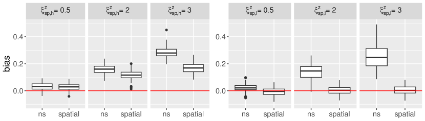
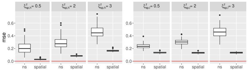
Figure 5: Bias (top) of $\widehat{\beta}$ and $\widehat{\beta}_{\mathrm{ns}}$ and MSE (bottom) of spatial and non-spatial (ns) models for high frequency (left) and low frequency (right) confounding. The true value is $\beta=0.5$. All other parameters remain constant.

B.2 Scenario 2: Confounding at Low Frequencies

In this scenario, we swap the weights of high and low frequencies in $\mathbf{z}$, such that there is only confounding at low frequencies. We consider $(\xi_{\mathrm{sp,l}}^{x},\xi_{\mathrm{sp,h}}^{x})=(1,1)$, $\xi_{\mathrm{sp,h}}^{z}=0$ and $\xi_{\mathrm{sp,l}}^{z}\in\{0.5,2,3\}$. The results in Figure 5 follow similarly to Scenario 2 in Section 4. When confounding only happens at low frequencies, the bias is close to zero in the spatial model and remains close to zero as $\xi_{\mathrm{sp,l}}^{z}$ increases, even despite potential model mis-specification. Thus, the thin plate splines generally seem able to capture the behavior of the GP used in the DGP. In contrast, the non-spatial model has a positive and linearly increasing bias, similar to Scenario 2, since all terms are weighted by $1$, as opposed to the spatial model where lower frequencies have lower weights.

B.3 Scenario 3: Confounding at High Frequencies, Low Correlation

We consider $\xi_{\mathrm{sp,h}}^{x}=1$, $\xi_{\mathrm{sp,l}}^{z}=0$, $\xi_{\mathrm{sp,l}}^{x}\in\{5,10\}$ and $\xi_{\mathrm{sp,h}}^{z}\in\{0.5,2,3\}$. The results in Figure 6 follow similarly to Scenario 3 in Section 4, in that by increasing $\xi_{\mathrm{sp,l}}^{x}$ we can reach scenarios where the non-spatial model has smaller bias than the spatial model, because the correlation between $\mathbf{x}$ and $\mathbf{z}$ is overall low (and thus non-spatial bias is low), but it is strong at high frequencies (inducing high spatial bias).

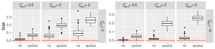
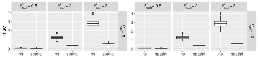
Figure 6: Bias (top) of $\widehat{\beta}$ and $\widehat{\beta}_{\mathrm{ns}}$ and MSE (bottom) of non-spatial (ns) and spatial models for different combinations of $\xi_{\mathrm{sp,h}}^{z}$ and $\xi_{\mathrm{sp,l}}^{x}$. The true value is $\beta=0.5$. All other parameters remain constant.

B.4 Scenario 4: Dependence on Non-Spatial Information

We consider $\sigma_{x}\in\{0.3,1,2,3\}$. Other parameters remain constant at $(\xi_{\mathrm{sp,l}}^{x},\xi_{\mathrm{sp,h}}^{x})=(1,1)$, $(\xi_{\mathrm{sp,l}}^{z},\xi_{\mathrm{sp,h}}^{z})=(0,2)$. The results in Figure 7 follow similarly to Scenario 4 in Section 4 and the bias decreases for both the non-spatial and spatial model when $\sigma_{x}$ is increased.

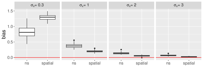
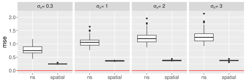
Figure 7: Bias (top) of $\widehat{\beta}$ and $\widehat{\beta}_{\mathrm{ns}}$ and MSE (bottom) of spatial and non-spatial models for different values of $\sigma_{x}$. The true value is $\beta=0.5$. All other parameters remain constant.

B.5 Scenario 5: Dependence on the Smoothing Parameter

We consider $(\xi_{\mathrm{sp,l}}^{x},\xi_{\mathrm{sp,h}}^{x})=(0,1)$, $(\xi_{\mathrm{sp,l}}^{z},\xi_{\mathrm{sp,h}}^{z})=(1,1)$, $\sigma_{x}=\sigma=1$, and fix $\lambda$ to different values. We let $\sigma_{x}\in\{0.3,1,2\}$. The results are based on 20 replicates.

As it can be observed in Figure 8, the higher the $\sigma_{x}$ the lower the bias. For $\sigma_{x}=0.3$, the spatial bias is mostly above the non-spatial bias and slowly converges to the non-spatial bias. Eventually, for $\sigma_{x}=2$, the spatial bias is always below the non-spatial bias, until it reaches it for large $\lambda$. Compared to Scenario 5 in Section 4, a bias close to 0 is never reached for $\sigma_{x}=0.3$, most likely due to the presence of additional mis-specification bias when using a GP as the DGP. The GCV estimate $\hat{\lambda}$ always stays on the steep part of the spatial bias curve, indicating that small changes in $\hat{\lambda}$ can lead to large changes in the spatial bias. The $\hat{\lambda}$ for the highest two $\sigma_{x}$ leads to a spatial bias lower than the non-spatial bias.

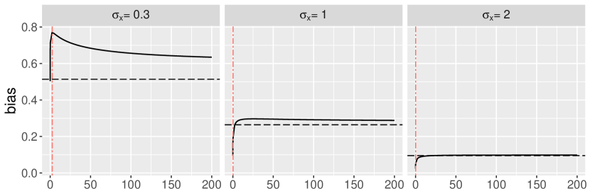
Figure 8: Bias of $\widehat{\beta}$ (solid black) and $\widehat{\beta}_{\mathrm{ns}}$ (dashed black) for increasing $\lambda$ and different $\sigma_{x}$. The true value is $\beta=0.5$. All other parameters remain constant. Magenta dashed line represents the median $\hat{\lambda}$ estimated by GCV. The bias associated with each $\hat{\lambda}$ is 0.7232, 0.1872, 0.0340, from left to right.

References

- Adin et al., (2023) Adin, A., Goicoa, T., Hodges, J. S., Schnell, P. M., and Ugarte, M. D. (2023). Alleviating confounding in spatio-temporal areal models with an application on crimes against women in india. Statistical Modelling, 23(1):9–30.
- Briz-Redón, (2023) Briz-Redón, Á. (2023). On alleviating spatial confounding issues with the Bayesian Lasso. Research Square preprint, doi:10.21203/rs.3.rs-2498913/v1.
- Clayton et al., (1993) Clayton, D. G., Bernardinelli, L., and Montomoli, C. (1993). Spatial correlation in ecological analysis. International Journal of Epidemiology, 22(6):1193–1202.
- Dupont et al., (2022) Dupont, E., Wood, S. N., and Augustin, N. (2022). Spatial+: A novel approach to spatial confounding. Biometrics, 78(4):1279–1290.
- Fahrmeir and Kneib, (2011) Fahrmeir, L. and Kneib, T. (2011). Bayesian Smoothing and Regression for Longitudinal, Spatial and Event History Data. Oxford University Press.
- Guan et al., (2023) Guan, Y., Page, G. L., Reich, B. J., Ventrucci, M., and Yang, S. (2023). Spectral adjustment for spatial confounding. Biometrika, 110(3):699––719.
- Hanks et al., (2015) Hanks, E. M., Schliep, E. M., Hooten, M. B., and Hoeting, J. A. (2015). Restricted spatial regression in practice: geostatistical models, confounding, and robustness under model misspecification. Environmetrics, 26(4):243–254.
- Hefley et al., (2017) Hefley, T. J., Hooten, M. B., Hanks, E. M., Russell, R. E., and Walsh, D. P. (2017). The bayesian group lasso for confounded spatial data. Journal of Agricultural, Biological and Environmental Statistics, 22(1):42–59.
- Hodges and Reich, (2010) Hodges, J. S. and Reich, B. J. (2010). Adding spatially-correlated errors can mess up the fixed effect you love. The American Statistician, 64(4):325–334.
- Hughes and Haran, (2013) Hughes, J. and Haran, M. (2013). Dimension reduction and alleviation of confounding for spatial generalized linear mixed models. Journal of the Royal Statistical Society: Series B (Statistical Methodology), 75(1):139–159.
- Keller and Szpiro, (2020) Keller, J. P. and Szpiro, A. A. (2020). Selecting a scale for spatial confounding adjustment. Journal of the Royal Statistical Society Series A: Statistics in Society, 183(3):1121–1143.
- Khan and Berrett, (2023) Khan, K. and Berrett, C. (2023). Re-thinking spatial confounding in spatial linear mixed models. arXiv preprint arXiv:2301.05743.
- Khan and Calder, (2022) Khan, K. and Calder, C. A. (2022). Restricted spatial regression methods: implications for inference. Journal of the American Statistical Association, 117(537):482–494.
- Marques et al., (2022) Marques, I., Kneib, T., and Klein, N. (2022). Mitigating spatial confounding by explicitly correlating gaussian random fields. Environmetrics, 33(5):e2727.
- Nobre et al., (2021) Nobre, W. S., Schmidt, A. M., and Pereira, J. B. M. (2021). On the effects of spatial confounding in hierarchical models. International Statistical Review, 89(2):302–322.
- Paciorek, (2010) Paciorek, C. J. (2010). The importance of scale for spatial-confounding bias and precision of spatial regression estimators. Statistical Science, 25(1):107–125.
- Page et al., (2017) Page, G. L., Liu, Y., He, Z., and Sun, D. (2017). Estimation and prediction in the presence of spatial confounding for spatial linear models. Scandinavian Journal of Statistics, 44(3):780–797.
- Papadogeorgou et al., (2019) Papadogeorgou, G., Choirat, C., and Zigler, C. M. (2019). Adjusting for unmeasured spatial confounding with distance adjusted propensity score matching. Biostatistics, 20(2):256–272.
- Reich et al., (2006) Reich, B. J., Hodges, J. S., and Zadnik, V. (2006). Effects of residual smoothing on the posterior of the fixed effects in disease-mapping models. Biometrics, 62(4):1197–1206.
- Reich et al., (2021) Reich, B. J., Yang, S., Guan, Y., Giffin, A. B., Miller, M. J., and Rappold, A. G. (2021). A review of spatial causal inference methods for environmental and epidemiological applications. International Statistical Review, 89(3):605–634.
- Schnell and Papadogeorgou, (2020) Schnell, P. M. and Papadogeorgou, G. (2020). Mitigating unobserved spatial confounding when estimating the effect of supermarket access on cardiovascular disease deaths. The Annals of Applied Statistics, 14(4):2069–2095.
- Thaden and Kneib, (2018) Thaden, H. and Kneib, T. (2018). Structural equation models for dealing with spatial confounding. The American Statistician, 72(3):239–252.
- Urdangarin Iztueta et al., (2022) Urdangarin Iztueta, A., Goicoa Mangado, T., and Ugarte Martínez, M. D. (2022). Evaluating recent methods to overcome spatial confounding. Revista Matemática Complutense 1-28.
- Wood, (2003) Wood, S. N. (2003). Thin plate regression splines. Journal of the Royal Statistical Society Series B: Statistical Methodology, 65(1):95–114.
- Zimmerman and Ver Hoef, (2022) Zimmerman, D. L. and Ver Hoef, J. M. (2022). On deconfounding spatial confounding in linear models. The American Statistician, 76(2):159–167.