Space-Time Attention with Shifted Non-Local Search

Abstract

Efficiently computing attention maps for videos is challenging due to the motion of objects between frames. While a standard non-local search is high-quality for a window surrounding each query point, the window’s small size cannot accommodate motion. Methods for long-range motion use an auxiliary network to predict the most similar key coordinates as offsets from each query location. However, accurately predicting this flow field of offsets remains challenging, even for large-scale networks. Small spatial inaccuracies significantly impact the attention module’s quality. This paper proposes a search strategy that combines the quality of a non-local search with the range of predicted offsets. The method, named Shifted Non-Local Search, executes a small grid search surrounding the predicted offsets to correct small spatial errors. Our method’s in-place computation consumes 10 times less memory and is over 3 times faster than previous work. Experimentally, correcting the small spatial errors improves the video frame alignment quality by over 3 dB PSNR. Our search upgrades existing space-time attention modules, which improves video denoising results by 0.30 dB PSNR for a 7.5% increase in overall runtime. We integrate our space-time attention module into a UNet-like architecture to achieve state-of-the-art results on video denoising.

1 Introduction

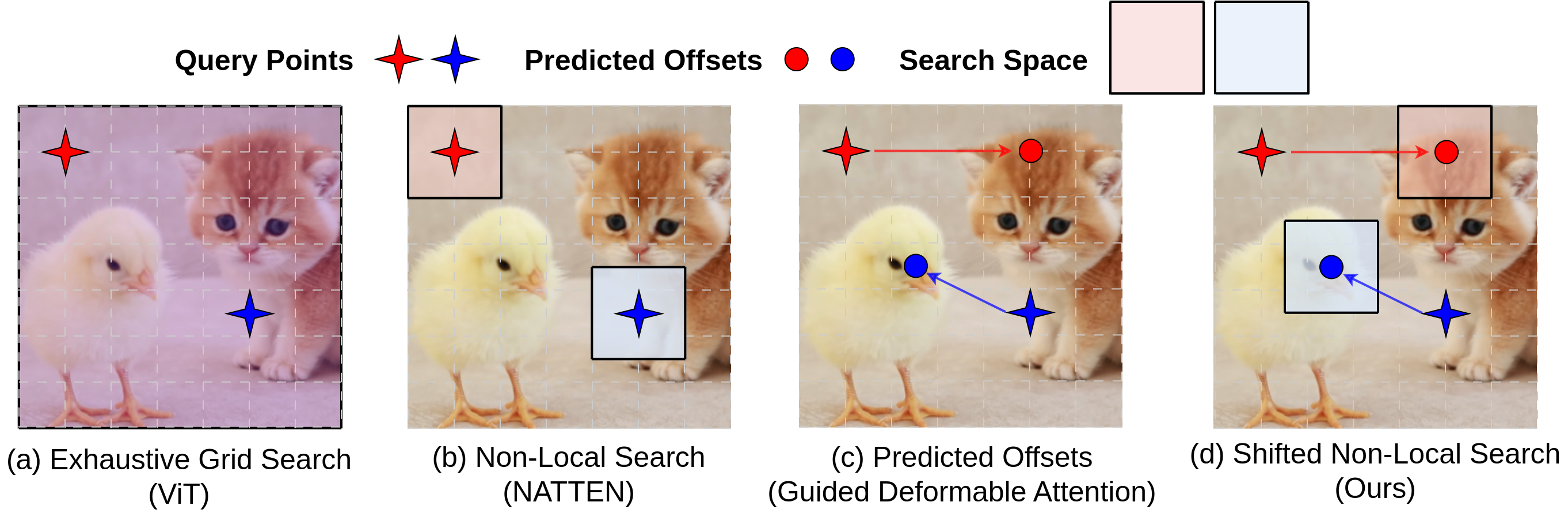
Figure 1: Comparing the Search Space of Attention Modules. (From left to right) ViT uses an exhaustive, global grid search which is computationally costly  (Dosovitskiy et al., 2020). A non-local search can be implemented efficiently but does not shift the search space according to the motion between frames (Hassani et al., 2023). The predicted offsets used in Guided Deformable Attention allow for long-range dependencies, but the flow fields contain small spatial inaccuracies (Liang et al., 2022b). Our method, the Shifted Non-Local Search, combines the quality of a non-local search with the range of predicted offsets. It executes a small grid search surrounding the predicted offsets to correct small spatial errors.

Attention modules form data-dependent receptive fields to aggregate related features from arbitrary coordinates. This functionality is considered to be central to the success of large-scale networks (Dosovitskiy et al., 2020; Hassani et al., 2023; Tian et al., 2020; Liang et al., 2022b). Recent efforts aggregate features across frames of a video, enabling deep networks to learn temporal representations of a scene. For images, the receptive fields are often bounded by a window surrounding the query location to reduce computation and the risk of overfitting. However, across frames of a video, this window must shift to data-dependent locations according to the motion. Long-range offsets are required, such as optical flow or nearest neighbors field (Barnes et al., 2010; Ranjan & Black, 2017a).

Non-local search strategies, such as NATTEN, provide excellent short-range receptive fields (Hassani et al., 2023). However, this category of method does not offset the search window, so it cannot handle the motion inherent to a space-time search. Alternative methods, such as Guided Deformable Attention, predict long-range offsets using an auxiliary network to accommodate motion (Liang et al., 2022b). However, accurately predicting flow fields remains an open challenge, even for large-scale networks (Butler et al., 2012).

This paper combines the quality of the non-local search with the range of predicted offsets. Our method, named Shifted Non-Local Search (Shifted-NLS), executes a small windowed grid search surrounding the predicted offset. For a marginal increase in wall-clock runtime, our search method acts as a correction step to the predicted offsets. In addition, our grid search is differentiable, which allows networks to learn long-range offsets. Our method works for attention because, unlike optical flow’s goal of estimating apparent motion, standard attention modules are defined through a grid search. We show our search method improves video alignment, upgrades existing space-time attention modules, and enables a state-of-the-art architecture for video denoising.

Critically, this paper also offers a practical means to compute the Shifted Non-Local Search. An important related work, named N3Net, already offers a similar method (Plötz & Roth, 2018). However, their method is not presented in the context of attention and requires integer-spaced indexing. Also, the N3Net search’s forward runtime is 3-7x slower than our search and requires over a 10-25x spike in GPU memory. These computational demands may explain why the module has not been adopted in recent works on space-time attention, and our Pytorch-friendly module offers a practical alternative (Paszke et al., 2019).

In summary, our contributions are: (i) We propose the shifted non-local search module for space-time attention. The module corrects spatial errors of predicted offsets using a high-fidelity windowed grid search. (ii) Our implementation uses in-place computation to reduce computational demands compared to previous work, using 10 times less memory and executing 3 times faster than N3Net (Plötz & Roth, 2018). While our code is not explicitly optimized for speed, our search’s runtime is only 1 - 2.5 times slower than an optimized space-only non-local search (Hassani et al., 2023). (iii) Our search method improves video alignment quality by more than 3 dB PSNR, yielding improved deep network quality for video denoising.

2 Related Works

Space-Only Attention: Attention modules often use a modified search space to be computationally efficient, and most of them search only spatially (Dosovitskiy et al., 2020; Mou et al., 2021; Liu et al., 2021). Hassani et al. (2023) offers an efficient non-local search but cannot accommodate long-range offsets. Xia et al. (2022) applies predicted offsets for single images but suffers from the inaccuracy of using a network to predict the flow field.

Space-Time Attention: Recent works propose temporal attention modules using predicted offsets learned with auxiliary networks which are inspired by Deformable Convolution (Dai et al., 2017). Examples of these methods include the temporal mutual self-attention module (TSMA), the temporal deformed alignment module (TDAN), and the guided deformable attention module (GDA) (Liang et al., 2022a; Tian et al., 2020; Liang et al., 2022b). Each method predicts pixel-level offsets and warps an adjacent frame to match a query frame. These methods all require training a network to learn these offsets. Plötz & Roth (2018) proposed N3Net which does execute a shifted grid search, but its implementation is not connected to attention modules, does not propagate gradients through its grid search, and requires expensive computation. Video Non-Local Bayes is a classical method that can be formulated as an attention module (Arias & Morel, 2018). Figure 1 compares the search space of related works on a single frame.

Restoration Architectures: Presented concurrently with new attention modules, authors often present an architecture design for video restoration. TDAN is used for video super-resolution, and RVRT is applied to video super-resolution, deblurring, and denoising (Tian et al., 2020; Liang et al., 2022b). Their attention only applies to frame pairs, while ours searches multiple frames in parallel.

3 Method

3.1 Problem Setup

The attention modules described in this section introduce increasingly sophisticated search methods to establish notation and illustrate how the Shifted Non-Local Search naturally extends related works.

Global Attention. An input video, ${\bm{X}}_{\text{in}}$, has shape $T\times H\times W\times F$ denoting frames, height, width, and features. The video is projected with a $1\times 1$ convolution to create the query (${\bm{Q}}$), key (${\bm{K}}$), and value (${\bm{V}}$) videos. When the videos are reshaped into matrices of size $THW\times F$, we use a subscript $M$, i.e. ${\bm{Q}}_{M}$. Attention consists of two steps: search and aggregate. Searching computes the similarity between the queries and keys, often using an outer product written as the matrix ${\bm{S}}={\bm{Q}}_{M}{\bm{K}}_{M}^{\intercal}$ with shape $THW\times THW$. Aggregation computes the weighted sum of key rows written as ${\bm{A}}=\sigma({\bm{S}}){\bm{V}}_{M}$ with shape $THW\times F$ where $\sigma(\cdot)$ is the softmax function applied across the columns. In summary, ${\bm{X}}_{\text{out}}=\text{Attention}({\bm{X}}_{\text{in}})=\text{reshape}(\sigma({\bm{Q}}_{M}{\bm{K}}_{M}^{\intercal}){\bm{V}}_{M})$ (Dosovitskiy et al., 2020). The global search requires expensive computation and is unnecessary for some applications.

Neighborhood Attention. Neighborhood Attention constructs a sparse similarity matrix by reducing the number of similarities computed between the queries and keys (Hassani et al., 2023). With specialized code, this attention is much faster than the global search and reduces the risk of overfitting. For each query, the similarity will only be computed for keys within a spatial window of size $(W_{s},W_{s})$ surrounding the query’s coordinate. To describe this in detail, we associate the $i^{\text{th}}$ row of the similarity matrix with the 3D coordinate at $(t_{i},h_{i},w_{i})$. The similarities are now computed as ${\bm{S}}[i,j]={\bm{Q}}_{M}[i]{\bm{K}}_{M}[j]^{\intercal}={\bm{Q}}[t_{i},h_{i},w_{i}]{\bm{K}}[t_{j},h_{j},w_{j}]^{\intercal}$ when $(t_{j},h_{j},w_{j})\in\left\{(t_{i},h_{i}-W_{s}/2+\delta_{h},w_{i}-W_{s}/2+\delta_{w}):\delta_{h},\delta_{w}\in\left\{0,\ldots,W_{s}-1\right\}\right\}$. Since most columns of ${\bm{S}}$ are zero, the data is restructured as ${\bm{S}}[i,\delta_{h},\delta_{w}]={\bm{Q}}[t_{i},h_{i},w_{i}]{\bm{K}}[t_{i},h_{i}-W_{s}/2+\delta_{h},w_{i}-W_{s}/2+\delta_{w}]^{\intercal}$.

The Non-Local Search. Rather than compute similarities between pixels, the standard non-local search from denoising literature operates on patches (Buades et al., 2011). Patches are more robust to noise than pixels and allow query coordinates to be skipped with an integer-valued query stride. The final output will be valid (e.g. no holes) when the patch size ($P$) and query stride ($S_{Q}$) satisfy the following condition, $\left\lfloor{(P-1)/2}\right\rfloor<S_{Q}$. To clean-up the messy indexing, we compactly write the spatial (height) index as $h_{i}(\delta_{h})=h_{i}-W_{s}/2+\delta_{h}$. Similarity values are now computed as ${\bm{S}}[i,\delta_{h},\delta_{w}]=\sum_{p_{h},p_{w}=-P/2,-P/2}^{P/2,P/2}{\bm{Q}}[t_{i},h_{i}+p_{h},w_{i}+p_{w}]{\bm{K}}[t_{i},h_{i}(\delta_{h}+p_{h}),w_{i}(\delta_{w}+p_{w})]^{\intercal}$ where $i\in\{0,\ldots,T(HW/S_{Q}^{2})-1\}$ so ${\bm{S}}$ has shape $THW/S_{Q}^{2}\times W_{s}\times W_{s}$.

3.2 The Shifted Non-Local Search

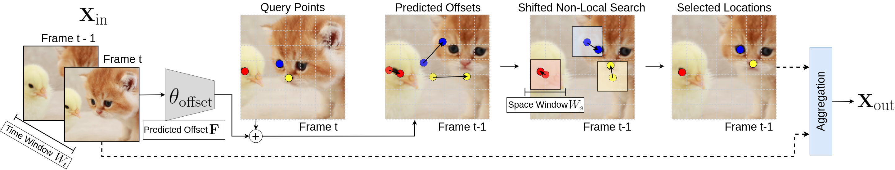
Figure 2: The Shifted Non-Local Search for Space-Time Attention. This figure depicts a space-time attention module using the Shifted Non-Local Search. The query points are deformed using the predicted offsets. Next, a grid search is executed surrounding the predicted offsets, and then the most similar locations are chosen from the search window. These locations are aggregated using a module such as Guided Deformable Attention.

The Shifted Non-Local Search. A Shifted Non-Local Search (Shifted-NLS) executes a Non-Local Search with the center of each spatial window shifted by an offset. The offsets between frames $t$ and $t-1$ are denoted as ${\bm{F}}_{\text{in}}$ with shape $T\times H\times W\times 2$. The center of the search window is shifted from $(h_{i},w_{i})$ to $(h_{i}+\Delta_{h}(i),w_{i}+\Delta_{w}(i))$ with $(\Delta_{h}(i),\Delta_{w}(i))={\bm{F}}_{\text{in}}[t_{i},h_{i},w_{i}]$. This shift is depicted in Figure 2 by the colored circles at the end of the arrows under “Predicted Offsets”. The similarities are computed as ${\bm{S}}[i,\delta_{h},\delta_{w}]=\sum_{p_{h},p_{w}=-P/2,-P/2}^{P/2,P/2}{\bm{Q}}[t_{i},h_{i},w_{i}]{\bm{K}}[t_{i}-1,h_{i}(\delta_{h}+p_{h})+\Delta_{h}(i),w_{i}(\delta_{w}+p_{w})+\Delta_{w}(i)]^{\intercal}$ using compact notation for the spatial (height) index, $h_{i}(\delta_{h})=h_{i}-W_{s}/2+\delta_{h}$. These offset search windows are depicted by the colored squares under “Shifted Non-Local Search” in Figure 2. The output offsets are the displacements from each query coordinate: ${\bm{F}}_{\text{out}}[i,\delta_{h},\delta_{w}]=(h_{i}(\delta_{h})+\Delta_{h}(i)-h_{i},w_{i}(\delta_{w})+\Delta_{w}(i)-w_{i})$.

Once the similarities are computed, we collapse the search dimensions ($W_{s}\times W_{s}$) into a single dimension ($W_{s}^{2}$) and retain only the top-L (aka “top-K”) most similar columns, ${\bm{S}}_{L},{\bm{F}}_{\text{out},L}=\text{top-L}({\bm{S}},{\bm{F}}_{\text{out}},L)$. The top-L operator has known theoretical issues with differentiation, but we observe networks still learn good weights despite this (Plötz & Roth, 2018). The top-L ($L=1$) coordinates are depicted under “Selected Locations” on the far right of Figure 2. This output is written as the similarity (${\bm{S}}_{L}$) and offset (${\bm{F}}_{\text{out},L}$) tensors with shapes $T(HW)/S_{Q}^{2}\times L$ and $T(HW)/S_{Q}^{2}\times L\times 2$, respectively. In summary: ${\bm{S}}_{L},{\bm{F}}_{\text{out},L}=\text{Shifted-NLS}({\bm{Q}},{\bm{K}},{\bm{F}}_{\text{in}},L)$.

In practice, the Shifted-NLS is computed in parallel across a temporal window of size $W_{t}$. Additionally, a key stride ($S_{K}$) changes the spacing between points in the grid search to allow for sub-pixel correction, $h_{i}(S_{K}\delta_{h}+p_{h})=h_{i}-S_{K}W_{s}/2+S_{K}\delta_{h}+p_{h}$. And since these coordinates are floating-points, bilinear interpolation is used for efficient indexing (Jeon & Kim, 2017).

Aggregation. The features from the Shifted-NLS are aggregated, and an example method is a weighted sum of non-local patches. The output video is initialized to zero, and each non-local patch is added in parallel (using atomic operators) weighted by a normalized similarity value. For example, writing the offsets as $(\Delta_{h}(i,l),\Delta_{w}(i,l))={\bm{F}}_{\text{out},L}[i,l]$, each patch’s $(p_{h},p_{w})$ pixel is added as ${\bm{X}}_{\text{out}}[t_{i},h_{i}+p_{h},w_{i}+p_{w}]\mathrel{+}=\sum_{l=1}^{L}\sigma({\bm{S}}_{L})[i,l]{\bm{V}}[t_{i}-1,h_{i}+\Delta_{h}(i,l)+p_{h},w_{i}+\Delta_{w}(i,l)+p_{w}]$, where $\sigma(\cdot)$ is the softmax function applied across the columns. Each pixel coordinate is divided by the number of contributing terms to normalize the output. When the patch size is $1$, this is logically identical to Guided Deformable Attention (GDA) (Liang et al., 2022b). And while the Shifted-NLS is compatible with GDA, GDA is limited to aggregating features from a single frame. For our Space-Time Attention Network (STAN) architecture, we would like to aggregate features across multiple frames in parallel according to learned weights, similar to PacNet (Vaksman et al., 2021). To implement this logic, we create a module to stack $L$ patches and apply 3D convolution to reduce the stack across $L$. Details are in Supplemental Section 7.

3.3 Why are predicted offsets not enough?

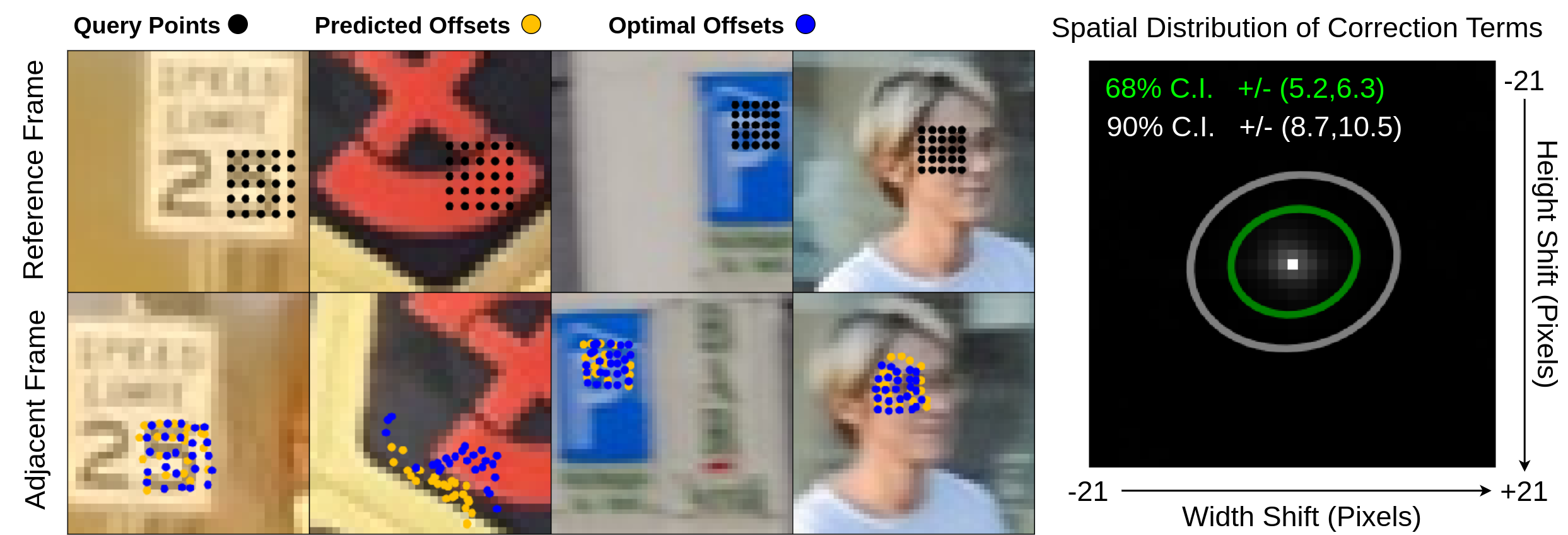
Figure 3: Predicted offsets are only a few pixels away from their optimal location. This figure shows query points in the query frame (top; black points), and their counterparts in the adjacent frame shifted with optical flow (bottom; blue points). The optical flow points are then corrected by a grid search of size $41\times 41$ (bottom; yellow points). The spatial similarity between the blue and yellow points show that repurposing optical flow estimates for attention requires only small spatial corrections. The right subfigure plots the distribution of these corrections. The peak value is positioned at the center, indicating no correction is necessary for 3.5% of all cases. The two ellipses form the 68% and 90% confidence intervals.

A Shifted Non-Local Search executes a grid search surrounding a predicted offset to correct spatial inaccuracies. In this section, we explain why even this simple grid search can intuitively outperform small networks by reviewing results in the closely related research area of optical flow.

Millions of parameters for a 6-pixel error. The best methods for optical flow today, according to the Sintel-Clean benchmark, report an average end-point error of about 1 pixel (Butler et al., 2012). Meanwhile, the classical pyramid-based method of 2014 reports an error of 6.73 pixels (Sun et al., 2014). Although the average improvement of about 6 pixels is impressive, this gap is closed using sophisticated training methods and network architectures with millions of parameters. Some applications claim to hugely benefit from the subpixel accuracy of these methods. However, it seems unlikely that each instance of an attention module will require its own auxiliary network with millions of parameters to simply predict coordinates with similar features.

Assessing the Error of Optical Flow for Attention. While the end-point-error is compared against an optical flow groundtruth, we qualitatively find the error to be similar when optical flow is used to estimate locations for attention. Using OpenCV’s implementation of Farneback’s optical flow method from 2003, Figure 3 qualitatively shows the flow’s errors are concentrated in a small region surrounding the initial estimate, despite a large search grid of size $41\times 41$ (Itseez, 2015; Farnebäck, 2003). This supports our idea to execute a small windowed grid search to correct the predicted offsets.

3.4 An Inplace Computation

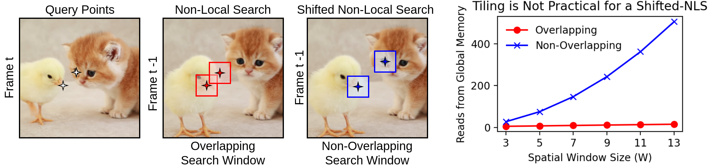
Figure 4: Video Dynamics Challenge Existing Computational Approaches. Searching across time is computationally challenging because spatially adjacent patches in one frame have data-dependent spatial locations in adjacent frames. This figure shows two neighboring locations in one frame (the chick and the kitten) move to separate spatial locations in the next frame. The benefit of NATTEN’s tiling is lost because the search windows no longer overlap (Hassani et al., 2023). The rightmost subfigure plots the number of global memory reads, highlighting the lost benefit of tiling.

Our In-Place Computation. Our in-place computation of the Shifted Non-Local Search executes each query-key pair’s similarity using the indexing from Section 3.2. The term in-place specifies our search does not require storing additional data related to the video. This is similar to NATTEN, but unlike N3Net which requires the construction of a patch database. However, NATTEN’s fixed-window search uses tiling to reduce the number of reads from global memory, which does not freely extend to a shifted search. Also, the global memory access pattern of a shifted window search is undesirable, which necessarily increases our method’s runtime. Section 4.4 shows despite this issue, our method is 3 - 7x faster than N3Net. In some cases, our search is even faster than NATTEN.

Limitations of NATTEN. NATTEN is designed to execute a non-local search with a small runtime (Hassani et al., 2023). Their core efficiency comes from reducing the number of reads from global memory by sharing global reads across the threads of a CUDA block. This principle does not freely extend to space-time because the search windows shift to data-dependent, non-overlapping locations, as depicted in Figure 4. Let $Q=3$ be the tiled size and $W_{s}$ as the window size; then overlapping windows require only $Q+W_{s}-1$ global reads while non-overlapping windows require $Q\cdot W_{s}^{2}$ global reads. The far-right subfigure in Figure 4 plots these two quantities, showing a significant disparity between the two cases. The necessarily increased number of global reads for a space-time search is a fundamental difference from space-only operators.

Limitations of N3Net. The query (${\bm{Q}}$) and key (${\bm{K}}$) videos can be unfolded to construct a database of patches, written as ${\bm{Q}}_{P}$ and ${\bm{K}}_{P}$ with shape $T(HW/S_{Q}^{2})\times FP^{2}$ and $T(HW/S_{K}^{2})\times FP^{2}$, respectively. The query ($S_{Q}$) and key ($S_{K}$) strides must be integer-valued. Normally, operators can batch across large dimensions, such as $T(HW/S_{K}^{2})$, to control memory consumption. However, the data-dependent indexing across space-time makes batching across the keys impossible. The entire key database must be simultaneously represented in memory since each query patch may access any key patch. If queries are searched in parallel, the memory consumption increases by $P^{2}\times\left(1/S_{Q}^{2}+1/S_{K}^{2}\right)$. For example, if $P=3$ and $S_{Q}=S_{K}=1$, the memory consumption of the videos increases by a factor of $18$.

4 Experiments

First, video alignment (Sec 4.1) demonstrates the Shifted Non-Local Search (Shifted-NLS) dramatically improves an attention module’s quality. Next (Sec 4.2), RVRT’s network is upgraded by replacing the Predicted Offsets with our Shifted-NLS, showing the improved attention module quality translates to improved denoising quality. Finally (Sec 4.3), RVRT’s pairwise frame restriction is lifted to a multi-frame network (STAN), which achieves state-of-the-art video denoising results.

4.1 Video Frame Alignment

The Shifted Non-Local Search (Shifted-NLS) corrects the small spatial errors of predicted offsets (e.g. optical flow). However, assessing these spatial errors by directly comparing the offsets is misleading. Since the offsets are subsequently used for aggregation, similar offsets can (and do) produce dissimilar outputs. Video alignment provides a ground-truth target for the attention module’s final output with standard qualitative and quantitative evaluation criteria.

For video alignment, we first execute the search with the queries set to frame $t$, ${\bm{Q}}={\bm{X}}_{\text{in}}[t]$, and keys and values set to frame $t+1$, ${\bm{K}}={\bm{V}}={\bm{X}}_{\text{in}}[t+1]$. Second, we aggregate using only the most similar patches (top-$L=1$). The output should match frame $t$ of the input, i.e. ${\bm{X}}_{\text{out}}\approx{\bm{X}}_{\text{in}}[t]$. This experiment uses the first 10 frames from the DAVIS training dataset (Pont-Tuset et al., 2017). When searching and computing the Farneback optical flow, we add a small amount of Gaussian noise ($\sigma^{2}=15$) to simulate the training dynamics between the query and key values (Farnebäck, 2003). Alignment quality is measured as the PSNR between the noise-free aligned and reference images. Both the Shifted-NLS and the Non-Local Search (NLS) methods use our implementation since NATTEN’s patch size is fixed to 1 and limited to a search space of $13$ $(W_{s}=13)$.

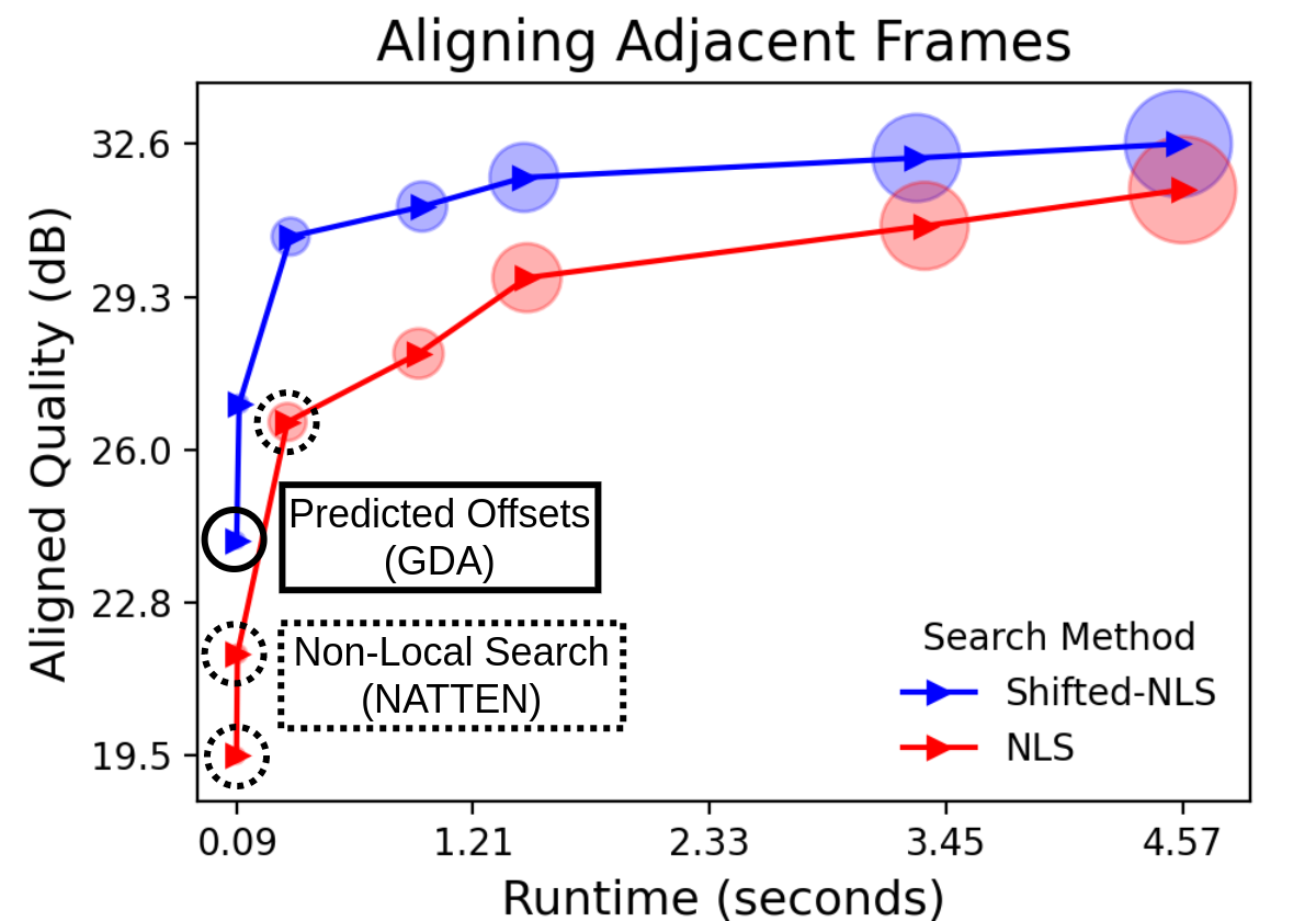
Figure 5: The Shifted-NLS Improves Alignment Quality. The Shifted-NLS achieves a better alignment with fewer search pixels than the NLS. Along each line the search window increases, $\{1,3,11,15,21,27,33\}$. The size of each point indicates the peak allocated memory when executing the search. A larger search grid is slower and consumes more memory.

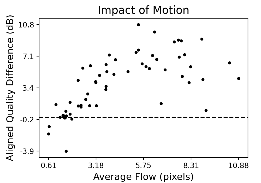
Figure 6: Video Motion Impacts the Alignment Quality. The y-axis plots the difference in the alignment quality between the Shifted-NLS and the NLS. The x-axis is an estimate of the video’s motion using the average absolute value of the optical flow. Each point represents a single video sequence. The dotted line is drawn at $0$ dB PSNR: no difference.

Figure 6 compares the alignment quality and runtime of the Shifted-NLS and the NLS as the search space expands. Each point is associated with a spatial window size, $W_{s}\in\{1,3,11,15,21,27,33\}$. A window of size 1 indicates no search. Currently, NATTEN supports window sizes up to $13$, as indicated by the dotted circles. For the Shifted-NLS, the PSNR plateaus around window size $11$, while for the NLS it plateaus around $21$. This matches our intuition that optical flow contains small spatial errors, which our grid search corrects. When the spatial search window is $11$, the Shifted-NLS yields $30.60$ dB PSNR while the NLS and the Predicted Offsets yield $26.63$ and $24.11$ dB PSNR, respectively. Figure 6 shows our Shifted-NLS method’s improvement depends on video motion. Each point is the difference in PSNR between the Shifted-NLS and the NLS for each video in the DAVIS training dataset. When motion is larger than about 3 pixels, Shifted-NLS improves the alignment quality by more than 5 dB PSNR. When the average motion is less than 1 pixel, the Shifted-NLS degrades the search quality. In the case of small motion, the offset values act as noise.

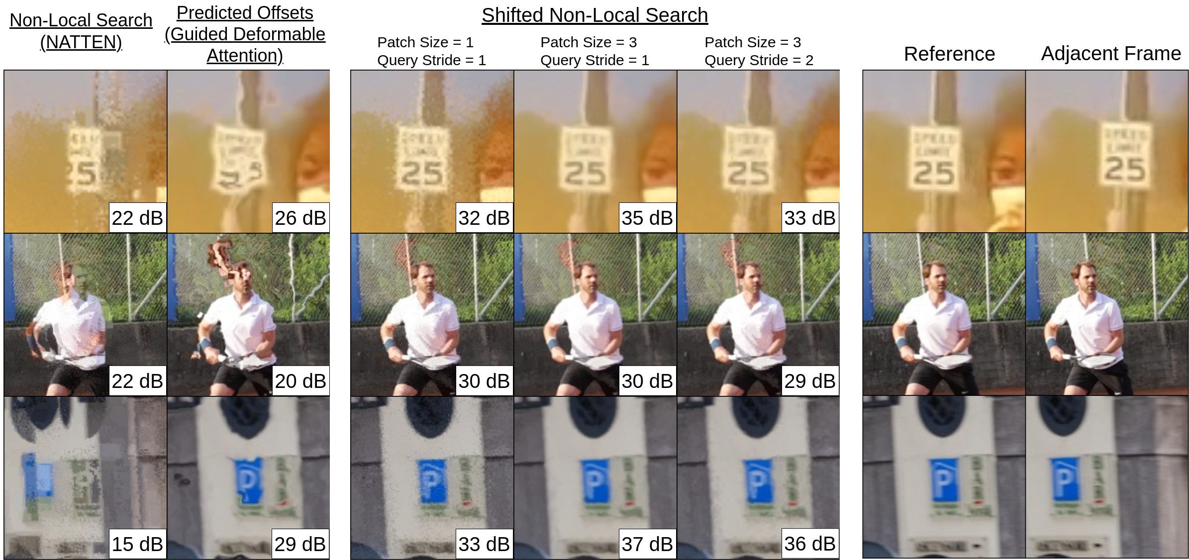
Figure 7: Comparing alignment quality for different search methods. This figure uses the indicated columns’s search method to align the adjacent frame (right) to the reference frame (second from right). The Non-Local Search and the Shifted Non-Local Search use a search space of $11\times 11$. The bottom-right corner reports the PSNR between the aligned and reference images; higher is better.

Figure 7 shows qualitative examples of the aligned images when the spatial search window is set to $11\times 11$. The NLS patch size is set to $1$ to match NATTEN, and the Shifted-NLS patch size and query stride is indicated in the column title. The NLS method creates a doubling effect because the search radius cannot compensate for the motion shifts. For example, the first number of the speed limit sign (top row) reads “5” rather than “2”. The Shifted-NLS largely removes the doubling effect, but not entirely. When the optical flow is inaccurate, a doubling effect still appears. For example, in the third row, a face appears where only a fence should be visible. The errors from Predicted Offsets create a warping effect similar to psychedelic art or the melting clocks of Salvador Dalí. The Shifted-NLS method visually removes the warping effect, replacing wavy edges with sharp ones.

Figure 7 also shows the impact of patch size and query stride. A larger patch size reduces noise since the overlapping patches are averaged together. This explains the qualitative difference between the grainy image with patch size 1 and the smoothed image with patch size 3. When the query stride is 2, patches no longer overlap producing the grainy output (middle row).

4.2 Upgrading Space-Time Attention

This experiment shows that replacing a small neural network with our Shifted Non-Local Search improves denoising quality. Guided Deformable Attention (GDA) uses an auxiliary network to produce offsets for aggregation by transforming an input video clip and optical flow offsets: ${\bm{F}}_{\text{out}}=\text{Auxiliary Network}({\bm{X}}_{\text{in}},{\bm{Y}}_{\text{in}},{\bm{F}}_{\text{in}})$. We replace their auxiliary network with our Shifted Non-Local Search: $\_,{\bm{F}}_{\text{out},L}=\text{Shifted-NLS}({\bm{X}}_{\text{in}},{\bm{Y}}_{\text{in}},{\bm{F}}_{\text{in}},L)$ with $L=9$ to match RVRT. The spatial window is $9\times 9$, the temporal window is fixed to $1$ by architecture design, the query stride is 1 ($S_{Q}=1$), the key stride is $1/2$ ($S_{K}=1/2$), and the patch size is 1. Table 1 shows the denoising quality improves when using our search method compared to using predicted offsets. The improvement is between $0.20-0.40$ dB across all noise levels, an increase often attributed to a new architecture.

Table 1: Upgrading Previous Space-Time Attention Modules. [PSNR$\uparrow$/SSIM$\uparrow$/ST-RRED$\downarrow$] This table reports denoising results on the DAVIS test dataset. RVRT’s GDA module aggregates features according to the input offsets. This table compares using the offsets from an auxiliary network (Predicted Offsets; the default) with a small grid search (Shifted-NLS).

$\sigma$	Predicted Offsets	Shifted-NLS
10	38.69/0.966/0.004	38.90/0.967/0.004
20	35.32/0.933/0.013	35.58/0.936/0.012
30	33.39/0.902/0.026	33.68/0.907/0.024
40	32.02/0.873/0.042	32.35/0.881/0.040
50	30.93/0.844/0.062	31.30/0.854/0.058
Time (sec)	23.86	25.56
Mem (GB)	10.06	10.06

4.3 Space-Time Attention Network (STAN)

We integrate the Shifted Non-Local Search into our Space-Time Attention Network (STAN). The architecture is a simple mixture of the UNet and RVRT networks (Ronneberger et al., 2015). We train the network for video denoising on the DAVIS train-val dataset (Pont-Tuset et al., 2017). We test the network on the DAVIS testing dataset and the Set8 dataset (Tassano et al., 2020). Due to space, we regulate details to Supplemental Section 6.4.

Table 2 shows our network achieves state-of-the-art results on video denoising. We note the original RVRT network reports better results, but we re-train RVRT to compare both networks trained on the same number of steps. This reproducibility problem may be due to the computational environment or insufficient training time (see Supplemental Section 6.4). However, we copy RVRT’s training procedure for both RVRT and STAN. Our method outperforms all other published video denoising methods, which supports the hypothesis that the Shifted Non-Local search is a useful module for space-time attention (Arias & Morel, 2018; Tassano et al., 2020; Vaksman et al., 2021).

Table 2: State-of-the-art Video Denoising. [PSNR$\uparrow$/SSIM$\uparrow$/ST-RRED$\downarrow$] This table reports state-of-the-art results on video denoising. *RVRT and STAN explicitly use space-time attention. The runtime and memory usage are recorded using a single 10-frame video of resolution $480\times 480$. We report reproduced RVRT results with further details in Supplemental Section 6.4.

	$\sigma^{2}$	VNLB	FastDVDNet	PaCNet	RVRT (Reproduced)*	STAN*
Set8	10	37.26	36.44	37.06	36.66/0.955/0.003	37.19/0.960/0.002
	20	33.72	33.43	33.94	33.47/0.918/0.011	34.27/0.931/0.007
	30	31.74	31.68	32.05	31.65/0.885/0.022	32.58/0.905/0.013
	40	30.39	30.46	30.70	30.38/0.855/0.035	31.39/0.880/0.021
	50	29.24	29.53	29.66	29.41/0.829/0.052	30.46/0.856/0.030
DAVIS	10	38.85	38.71	39.97	39.29/0.970/0.003	40.22/0.976/0.002
	20	35.68	35.77	36.82	36.00/0.942/0.010	37.30/0.956/0.007
	30	33.73	34.04	34.79	34.12/0.915/0.021	35.54/0.937/0.012
	40	32.32	32.82	33.34	32.80/0.891/0.034	34.26/0.918/0.020
	50	31.13	31.86	32.20	31.78/0.868/0.050	33.26/0.901/0.029
Time (sec)		497.93	0.11	182.34	1.63	3.26
GPU Memory (GB)		0.0	0.37	12.35	4.25	10.75
Parameters ($10^{6}$)		N/A	2.4	2.9	12.8	12.1

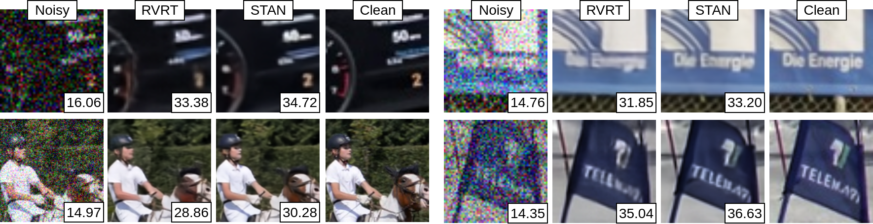
Figure 8: Qualitatively Comparing Denoised Outputs. [PSNR$\uparrow$] RVRT and STAN use space-time attention and are trained using the same procedure. STAN recovers more small details than RVRT.

4.4 Computational Benchmarking

This section compares the computation for three non-local search strategies. The Shifted-NLS and N3Net methods execute a space-time search, and NATTEN executes a space-only (unshifted) search. Each benchmark includes a function call to a top-L function for compatibility with existing aggregation methods. Figures 9 and 10 report benchmark results of each search method executed on a $5$ frame video with varying resolution. Due to NATTEN’s tiling, its query stride is fixed at $1$. The other methods vary the query stride to $1$ or $2$ as indicated by the dotted and solid lines, respectively.

Figure 9: The Shifted-NLS Consumes Less Memory. Our Shifted Non-Local Search module consumes less than $20\times$ the memory of N3Net’s search method and half the memory of NATTEN. N3Net expands the video into a database of patches, which requires an absurd consumption of GPU memory. NATTEN searches only pairs of frames, so the temporal search space must be stacked along the batch dimension.

Figure 10: The Runtime of Shifted-NLS is Competitive. NATTEN is a space-only search but serves as a competitive baseline. Importantly, NATTEN’s efficient tiling requires a query stride of $1$, unlike both other search methods. The Shifted-NLS method is $2.4$ times slower than NATTEN when the query stride is $1$, but it is $2$ times faster when the query stride is $2$.

Figure 9 reports memory consumption for an input video with $192$ features (such as in RVRT) using images with resolution $152\times 152$. Both N3Net and Shifted-NLS use a patch size of $7$. N3Net requires dramatically more memory than the Shifted-NLS module since it explicitly constructs a database of patches. When the spatial window size is 3, N3Net consumes 12.43 GB of memory, while the Shifted-NLS consumes 0.33 GB of memory. NATTEN’s memory consumption grows from about $0.75$ GB to $0.97$ GB. NATTEN searches pairs of frames, so parallel searching across space-time requires stacking frames of the temporal search window along the batch dimension.

Figure 10 reports runtimes using images with resolution $320\times 320$, a search window of size $9$, and a patch size of $1$. As expected, the Shifted-NLS module is slower than NATTEN when the query stride is fixed to $1$. For example, when the number of features is 32 the runtime of NATTEN and Shifted-NLS is about $36.77$ and $84.36$ milliseconds (ms), respectively. N3Net is far slower than both methods; N3Net’s runtime for a query stride of $1$ is too slow to plot clearly (about 490 ms). Notably, the Shifted-NLS is faster than NATTEN when the query stride can be set to $2$. For 32 features, the runtime of the Shifted-NLS drops from $84.36$ to $27.95$ ms. However, the search quality will degrade as the query stride increases so the utility of this faster runtime depends on the application.

5 Conclusion

This paper presents a Shifted Non-Local Search module for space-time attention. We first observe the errors of offsets predicted from auxiliary networks require only small spatial corrections. Rather than train a large-scale network with millions of parameters, we propose using a small grid search to correct these errors. Our in-place implementation of the Shifted Non-Local Search avoids absurd memory spikes with a competitive runtime. Correcting the small spatial errors corresponds to over a 3 dB improvement when aligning adjacent frames. We show this translates to improved denoising quality within denoising networks. As this module is designed for learning temporal representations, future work can apply this method to additional computer vision tasks such as instance segmentation and video synthesis.

6 Additional Experiments and Details

6.1 Dataset Summary

Our experiments use the DAVIS and Set8 datasets datasets (Pont-Tuset et al., 2017; Tassano et al., 2020). The DAVIS train-val dataset consists of 90 sequences and the number of frames in a sequence varies from $40$ - $104$ with resolution $480\times 854$. The DAVIS testing dataset consists of $30$ sequences. Set8 consists of four sequences from a GoPro camera and four sequences from the DAVIS test set. For Set8, the number of frames in a sequence varies from $35$ - $85$ with resolution $540\times 960$.

6.2 Upgrading Space-Only Attention

Is Losing Spatial Resolution Worth Space-Time Features? In practice, space-time attention might replace space-only attention. Is the loss of spatial information worth the temporal information? Theoretically assessing the impact of losing spatial information on model quality is difficult, so we instead seek experimental evidence. Using the COLA-Net architecture for video denoising, we find that space-time attention is significantly better than global or non-local space-only attention.

Experimental Details. We finetune the COLA-Net denoising network provided by the original authors for 30 epochs of 400 randomly selected sample sequences from the DAVIS training dataset (Pont-Tuset et al., 2017). Each sequence consists of $5$ frames with resolution $128\times 128$. We train on two Titan RTX GPUs with a batch size of $8$ using PyTorch Lightning (Falcon et al., 2019). The optimizer is Adam with a learning rate of $1\cdot 10^{-4}$ and the learning rate scheduler is stepped (e.g. StepLR) with a step size of $5$ and decay rate $\gamma=0.1$ (Kingma & Ba, 2014). As a control, we finetune the original model and observe no meaningful change in denoising quality.

Space-Time Features are Better than Space-Only Features for Denoising. Table 3 tests the network on DAVIS validation set where the column indicates the attention module and each row indicates the Gaussian noise intensity ($\sigma$) (Pont-Tuset et al., 2017; Mou et al., 2021). COLA-Net originally uses cross-scale attention, which is a global, strided search. The results in Table 3 show space-time non-local attention with optical flow outperforms the original network by over $1$ dB PSNR, and it is the best of all the attention modules. Figure 11 shows qualitative examples. The space-time search and the space-time attention module use a spatial window of size $15\times 15$, a patch size of $7$, and a query stride of $4$. The space-time search uses a temporal window of size $2$. We aggregate the non-local patches as a weighted sum of patches. Since denoising inherently depends on a local region of pixels, the usefulness of space-time features may be expected. The utility of space-time features remains unclear for tasks depending on semantic information, which is often spread globally across the image.

Space-Time Attention is Faster Than Global Attention. Table 3’s runtime and memory consumption is measured using a $5$ frame video of resolution $230\times 230$. This is the largest input video which fits on our 24 GB NVIDIA RTX 3090 GPU. The global attention module is over 3.5 times slower than our space-time search and consumes almost 20 times more memory. The space-only and space-time searches use our Shifted Non-Local Search module with a temporal window size of $1$ and $5$, respectively.

Table 3: Upgrading Search-Only Search. [PSNR$\uparrow$/SSIM$\uparrow$/ST-RRED$\downarrow$] This table reports denoising results on the DAVIS dataset using various attention modules within COLA-Net. The original attention module uses a global, strided search named cross-scale attention. We report results using the noise intensities ($\sigma^{2}$) to match the original paper.

Dataset	$\sigma$	Original (Global)	Non-Local Search	Shifted-NLS
DAVIS	15	34.26/0.915/1.3	34.14/0.912/1.4	35.78/0.936/0.8
	30	30.93/0.848/5.2	30.80/0.843/5.3	32.41/0.878/2.6
	50	28.67/0.784/13.6	28.51/0.776/13.5	29.73/0.810/7.2
Runtime (seconds)		1.703	0.242	0.439
Memory (GB)		14.449	0.730	0.736

Figure 11: Qualitatively Comparing Denoised Outputs. [PSNR$\uparrow$] Replacing COLA-Net’s global, cross-scale attention with both the space-only and space-time search impacts restoration quality. The space-time search can restore details not available from a single frame.

6.3 Upgrading Space-Time Attention: Additional Details

Upgrading Guided Deformable Attention. A Guided Deformable Attention (GDA) module requires offsets, denoted ${\bm{F}}_{\text{out}}$, with shape $H\times W\times 9\times 2$ where ${\bm{F}}_{\text{out}}[h_{i},w_{i},l]$ is the $(x,y)$ shift from $(h_{i},w_{i})$ between frames $t-1$ and $t$. These offsets are output from a network whose input includes a single optical-flow-like offset, denoted ${\bm{F}}_{\text{in}}$ with shape $H\times W\times 2$, and input clips ${\bm{X}}_{\text{in}},{\bm{Y}}_{\text{in}}$. Written another way, ${\bm{F}}_{\text{out}}=\text{Auxiliary Network}({\bm{X}}_{\text{in}},{\bm{Y}}_{\text{in}},{\bm{F}}_{\text{in}})$. We replace the network with our Shifted Non-Local Search: $\_,{\bm{F}}_{\text{out},L}=\text{Shifted-NLS}({\bm{X}}_{\text{in}},{\bm{Y}}_{\text{in}},{\bm{F}}_{\text{in}},L)$ with $L=9$ to match RVRT.

Training Details. The upgraded RVRT networks are trained for 90,000 iterations with a batch size of 8 with 10 frames each at resolution $256\times 256$. Each batch is corrupted with Gaussian noise using a random noise parameter, $\sigma\sim\text{Uniform}[0,50]$. Weight updates use the Adam optimizer with an initial learning rate of $4\times 10^{-4}$ and decrease with the Cosine Annealing learning rate scheduler (Kingma & Ba, 2014; Loshchilov & Hutter, 2016). RVRT’s internal SpyNet model is initialized with pre-trained weights which are fixed for the first 30,000 iterations and learns with a 75% reduced learning rate. (Ranjan & Black, 2017b; Niklaus, 2018). Notably, we execute only 90,000 iterations instead of 600,000 due to limited computing resources.

Ablation Study. Our Shifted Non-Local Search uses hyperparameters not learned during network training. To better understand their impact on video denoising quality, we train networks for various configurations. The search stride, $S_{K}$, denotes the spacing between two points in the grid search. When $S_{K}=0.5$ or $S_{K}=1$, then each grid point is spaced $1/2$ or $1$ pixel apart, respectively. Table 4 shows the results for a various number of search parameters. The best settings used a search stride of $0.5$ and a spatial window of $9$, outperforming the same window size with a search stride of $1$. This suggests subpixel corrections to the predicted offsets may be more beneficial than a larger search radius. A search radius that is too large or too small also decreases the network quality. We hypothesis a large search radius will overfit to noise and a small radius is insufficient to properly correct errors.

Table 4: Ablation Experiments for Shifted Non-Local Search.[PSNR$\uparrow$/SSIM$\uparrow$/ST-RRED$\downarrow$] A small spatial window ($W_{s}=3$) is unable to correct errors and a large spatial window ($W_{s}=15$) overfits to noise. A fractional search stride allows for subpixel correction.

$\sigma$	$W_{s}=9,S_{K}=0.5$	$W_{s}=9,S_{K}=1$	$W_{s}=15,S_{K}=1$	$W_{s}=3,S_{K}=1$
10	38.90/0.967/0.004	38.77/0.967/0.004	38.68/0.966/0.004	38.61/0.965/0.004
20	35.58/0.936/0.012	35.40/0.934/0.013	35.27/0.933/0.013	35.23/0.932/0.013
30	33.68/0.907/0.024	33.44/0.904/0.025	33.29/0.901/0.026	33.27/0.900/0.026
40	32.35/0.881/0.040	32.07/0.875/0.042	31.89/0.872/0.043	31.87/0.871/0.044
50	31.30/0.880/0.027	30.97/0.847/0.061	30.78/0.843/0.063	30.76/0.841/0.064

6.4 Space-Time Attention Network (STAN) for Video Denoising

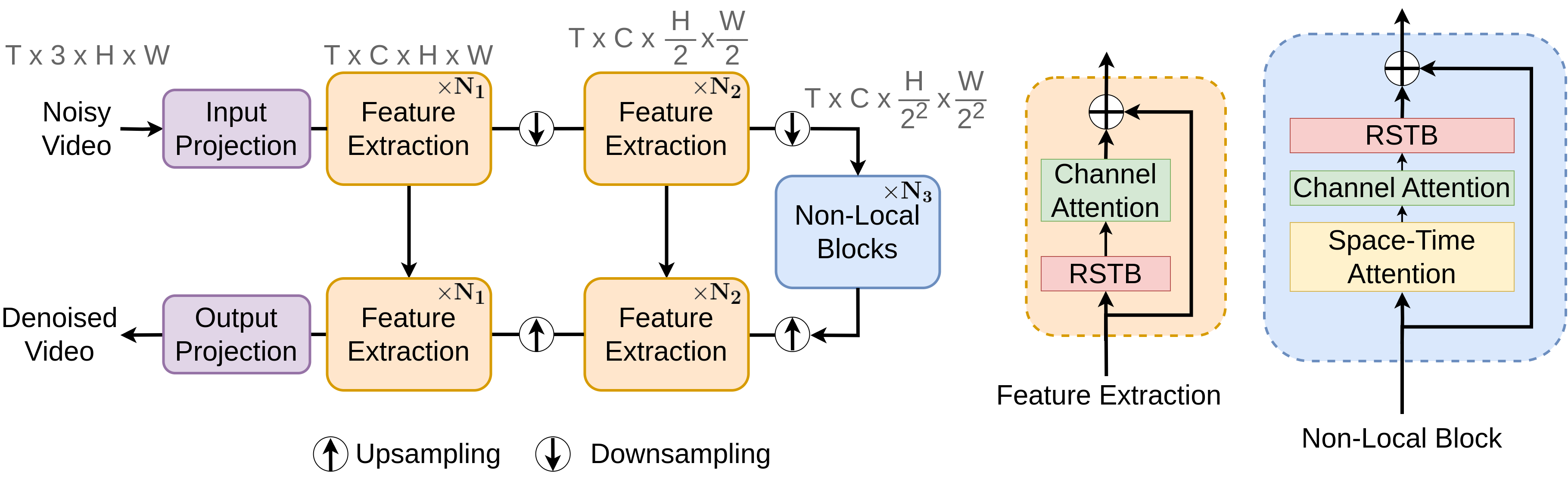
Figure 12: Space-Time Attention Network (STAN) Architecture. The STAN macro-level architecture design is inspired from UNet (Ronneberger et al., 2015). Each block’s design is inspired by the RVRT network (Liang et al., 2022b).

Architecture. The macro-level architecture is designed to match the multi-scale architecture of UNet (Ronneberger et al., 2015). Each non-local block contains layer normalization, our space-time attention module, channel attention, and lastly Residual Swin Transformer Blocks (Hu et al., 2018; Liang et al., 2021). The block structure is inspired by the RVRT network (Liang et al., 2022b). The space-time attention layer is described in Section 3.1, and we use the aggregation scheme described Section 3.2. Notably, there are no positional embeddings. Our networks are set to $N_{1}=1$, $N_{2}=2$, and $N_{3}=4$ with 1, 4, and 12 heads. STAN uses TV-L1 for optical flow (Zach et al., 2007). Only the first non-local block executes the space-time search while subsequent blocks use the previous layer’s top-L offsets.

Experimental Details. The RVRT and STAN networks are trained for 240,000 iterations with a batch size of 8 using clip lengths of 16 with resolution $256\times 256$. Each batch is corrupted with Gaussian noise using a random noise parameter, $\sigma\sim\text{Uniform}[0,50]$. Weight updates use the Adam optimizer with an initial learning rate of $4\times 10^{-4}$ and decrease with the Cosine Annealing learning rate scheduler (Kingma & Ba, 2014; Loshchilov & Hutter, 2016). The internal SpyNet model is initialized with pre-trained weights which are fixed for the first 30,000 iterations and uses a learning rate reduced by 75%. (Ranjan & Black, 2017b; Niklaus, 2018). Notably, we executed only 240,000 iterations instead of 600,000 due to limited computing resources. Because our lab operates on a time-limited SLURM computer restricted to 4 GPUs, training time changes from 21 to 90 days, depending on the server’s scheduler. Perhaps more than doubling the training time would close the gap of over 1 dB difference.

Reproducibility Description. While the authors of RVRT do not provide training code, a procedure is described in their paper. When following their training procedure, the network’s quality is significantly worse than their original report. An open issue on RVRT’s GitHub also reports a reproducibility issue. Since training a single RVRT network takes approximately 10 days, which costs about $5,875 on AWS, we do not have the resources for further investigation. Additionally, our SLURM-based training environment may cause issues. We use 4 GPUs for 4-hour increments, restoring the training state between each launch. While this functionality is explicitly supported by open source code, bugs are still reported (example issue 1 and issue 2).

Valid Conclusions Despite the Non-Reproducible Related Work. While we cannot reproduce the results from RVRT, we believe this does not change conclusions regarding our Shifted Non-Local Search module. Since the training procedure is copied directly from the RVRT paper and the procedure is identical for both RVRT and STAN, we have shown the value of a Shifted-NLS.

Ablation Experiment. We include an ablation study to assess the impact of space-time attention’s temporal window size in Table 5. Each column’s configuration is trained from scratch for $90,000$ epochs, following the training procedure previously described. The testing dataset is Set8.

Table 5: The Impact of the Temporal Windows. [PSNR$\uparrow$/SSIM$\uparrow$/ST-RRED$\downarrow$] The temporal window size changes the denoising quality of the STAN architecture. The temporal window size is the number of frames searched for each query point from each frame. When $W_{t}=1$, no adjacent frames are searched.

$\sigma$	$W_{t}=5$	$W_{t}=3$	$W_{t}=1$
10	36.71/0.957/0.003	36.59/0.956/0.003	36.42/0.953/0.003
20	33.94/0.927/0.008	33.77/0.925/0.008	33.51/0.920/0.009
30	32.29/0.900/0.014	32.10/0.896/0.015	31.82/0.890/0.016
40	31.11/0.874/0.023	30.92/0.870/0.024	30.74/0.862/0.026
50	30.19/0.850/0.033	30.00/0.845/0.035	29.72/0.838/0.038

7 Pytorch Example of Space-Time Attention

⬇

# – imports –

import torch as th

conv2d = th.nn.functional.conv2d

conv3d = th.nn.functional.conv3d

from einops import rearrange

import stnls

\par# -=-=-=-=-=-=-=-=-=-=-=-=-

# Init

# -=-=-=-=-=-=-=-=-=-=-=-=-

\par# – search & aggregate info –

ws = 5 # spatial window size

wt = 2 # temporal window size; searching total frames W_t = 2*wt+1

ps,K,HD = 3,10,2 # patch size, num of neighbors (aka ”L”), num of heads

stride0,stride1 = 1,0.5 # query & key stride

\par# – input video –

B,T,F,H,W = 1,5,16,128,128 # batch size, frames, features, height, width

device = ”cuda”

V_in = th.randn((B,T,F,H,W),device=device)

vshape = V_in.shape

\par# – optical flows –

fflow = th.randn((B,T,2,H,W),device=device)

bflow = th.randn((B,T,2,H,W),device=device)

\par# -=-=-=-=-=-=-=-=-=-=-=-=-

# Attention

# -=-=-=-=-=-=-=-=-=-=-=-=-

\par# – transform –

proj_weights = th.randn((F,F,1,1),device=device)

q_vid = conv2d(V_in.view(-1,*vshape[2:]),proj_weights).view(vshape)

k_vid = conv2d(V_in.view(-1,*vshape[2:]),proj_weights).view(vshape)

v_vid = conv2d(V_in.view(-1,*vshape[2:]),proj_weights).view(vshape)

\par# – search –

search = stnls.search.NonLocalSearch(ws,wt,ps,K,nheads=HD,

stride0=stride0,stride1=stride1)

dists,inds = search(q_vid,k_vid,fflow,bflow)

# print(inds.shape) # B,HD,T,nH,nW,K,3; nH=(H-1)//stride0+1

\par# – normalize –

weights = th.nn.functional.softmax(-10*dists,-1)

\par# – aggregate –

gather_nl = stnls.agg.NonLocalGather(ps,stride0)

stacked = gather_nl(v_vid,weights,inds)

# stacked.shape = (B,HD,K,T,F’,H,W) where F’ = F/HD

V_out = rearrange(stacked,’b hd k t f h w -> (b t) (hd f) k h w’)

proj_weights = th.randn((F,F,K,1,1),device=device)

V_out = conv3d(V_out,proj_weights,stride=(K,1,1))

V_out = rearrange(V_out,’(b t) f 1 h w -> b t f h w’,b=B)

# print(”V_out.shape: ”,V_out.shape) # B,T,F,H,W

References

- Arias & Morel (2018) Pablo Arias and Jean-Michel Morel. Video denoising via empirical bayesian estimation of space-time patches. Journal of Mathematical Imaging and Vision, 60(1):70–93, 2018.
- Barnes et al. (2010) Connelly Barnes, Eli Shechtman, Dan B Goldman, and Adam Finkelstein. The generalized patchmatch correspondence algorithm. In Proceedings of the European Conference on Computer Vision, pp. 29–43. Springer, 2010.
- Buades et al. (2011) Antoni Buades, Bartomeu Coll, and Jean-Michel Morel. Non-local means denoising. Image Processing On Line, 1:208–212, 2011.
- Butler et al. (2012) D. J. Butler, J. Wulff, G. B. Stanley, and M. J. Black. A naturalistic open source movie for optical flow evaluation. In A. Fitzgibbon et al. (Eds.) (ed.), Proceedings of the European Conference on Computer Vision, Part IV, LNCS 7577, pp. 611–625. Springer-Verlag, October 2012.
- Dai et al. (2017) Jifeng Dai, Haozhi Qi, Yuwen Xiong, Yi Li, Guodong Zhang, Han Hu, and Yichen Wei. Deformable convolutional networks. In Proceedings of the IEEE International Conference on Computer Vision, pp. 764–773, 2017.
- Dosovitskiy et al. (2020) Alexey Dosovitskiy, Lucas Beyer, Alexander Kolesnikov, Dirk Weissenborn, Xiaohua Zhai, Thomas Unterthiner, Mostafa Dehghani, Matthias Minderer, Georg Heigold, Sylvain Gelly, et al. An image is worth 16x16 words: Transformers for image recognition at scale. arXiv preprint arXiv:2010.11929, 2020.
- Falcon et al. (2019) William Falcon et al. Pytorch lightning. GitHub. Note: https://github.com/PyTorchLightning/pytorch-lightning, 3, 2019.
- Farnebäck (2003) Gunnar Farnebäck. Two-frame motion estimation based on polynomial expansion. In Image Analysis: 13th Scandinavian Conference, SCIA 2003 Halmstad, Sweden, June 29–July 2, 2003 Proceedings 13, pp. 363–370. Springer, 2003.
- Hassani et al. (2023) Ali Hassani, Steven Walton, Jiachen Li, Shen Li, and Humphrey Shi. Neighborhood attention transformer. In Proceedings of the IEEE/CVF Conference on Computer Vision and Pattern Recognition, pp. 6185–6194, 2023.
- Hu et al. (2018) Jie Hu, Li Shen, and Gang Sun. Squeeze-and-excitation networks. In Proceedings of the IEEE Conference on Computer Vision and Pattern Recognition, pp. 7132–7141, 2018.
- Itseez (2015) Itseez. Open source computer vision library. https://github.com/itseez/opencv, 2015.
- Jeon & Kim (2017) Yunho Jeon and Junmo Kim. Active convolution: Learning the shape of convolution for image classification. In Proceedings of the IEEE Conference on Computer Vision and Pattern Recognition, pp. 4201–4209, 2017.
- Kingma & Ba (2014) Diederik P Kingma and Jimmy Ba. Adam: A method for stochastic optimization. arXiv preprint arXiv:1412.6980, 2014.
- Liang et al. (2021) Jingyun Liang, Jiezhang Cao, Guolei Sun, Kai Zhang, Luc Van Gool, and Radu Timofte. Swinir: Image restoration using swin transformer. In Proceedings of the IEEE/CVF International Conference on Computer Vision, pp. 1833–1844, 2021.
- Liang et al. (2022a) Jingyun Liang, Jiezhang Cao, Yuchen Fan, Kai Zhang, Rakesh Ranjan, Yawei Li, Radu Timofte, and Luc Van Gool. Vrt: A video restoration transformer. arXiv preprint arXiv:2201.12288, 2022a.
- Liang et al. (2022b) Jingyun Liang, Yuchen Fan, Xiaoyu Xiang, Rakesh Ranjan, Eddy Ilg, Simon Green, Jiezhang Cao, Kai Zhang, Radu Timofte, and Luc V Gool. Recurrent video restoration transformer with guided deformable attention. Advances in Neural Information Processing Systems, 35:378–393, 2022b.
- Liu et al. (2021) Ze Liu, Yutong Lin, Yue Cao, Han Hu, Yixuan Wei, Zheng Zhang, Stephen Lin, and Baining Guo. Swin transformer: Hierarchical vision transformer using shifted windows. In Proceedings of the IEEE/CVF International Conference on Computer Vision, pp. 10012–10022, 2021.
- Loshchilov & Hutter (2016) Ilya Loshchilov and Frank Hutter. Sgdr: Stochastic gradient descent with warm restarts. arXiv preprint arXiv:1608.03983, 2016.
- Mou et al. (2021) Chong Mou, Jian Zhang, Xiaopeng Fan, Hangfan Liu, and Ronggang Wang. Cola-net: Collaborative attention network for image restoration. IEEE Transactions on Multimedia, 24:1366–1377, 2021.
- Niklaus (2018) Simon Niklaus. A reimplementation of SPyNet using PyTorch. https://github.com/sniklaus/pytorch-spynet, 2018.
- Paszke et al. (2019) Adam Paszke, Sam Gross, Francisco Massa, Adam Lerer, James Bradbury, Gregory Chanan, Trevor Killeen, Zeming Lin, Natalia Gimelshein, Luca Antiga, Alban Desmaison, Andreas Kopf, Edward Yang, Zachary DeVito, Martin Raison, Alykhan Tejani, Sasank Chilamkurthy, Benoit Steiner, Lu Fang, Junjie Bai, and Soumith Chintala. Pytorch: An imperative style, high-performance deep learning library. In H. Wallach, H. Larochelle, A. Beygelzimer, F. d'Alché-Buc, E. Fox, and R. Garnett (eds.), Advances in Neural Information Processing Systems 32, pp. 8024–8035. Curran Associates, Inc., 2019.
- Plötz & Roth (2018) Tobias Plötz and Stefan Roth. Neural nearest neighbors networks. Advances in Neural Information Processing Systems, 31, 2018.
- Pont-Tuset et al. (2017) Jordi Pont-Tuset, Federico Perazzi, Sergi Caelles, Pablo Arbeláez, Alexander Sorkine-Hornung, and Luc Van Gool. The 2017 davis challenge on video object segmentation. arXiv:1704.00675, 2017.
- Ranjan & Black (2017a) Anurag Ranjan and Michael J Black. Optical flow estimation using a spatial pyramid network. In Proceedings of the IEEE Conference on Computer Vision and Pattern Recognition, pp. 4161–4170, 2017a.
- Ranjan & Black (2017b) Anurag Ranjan and Michael J. Black. Optical flow estimation using a spatial pyramid network. In IEEE Conference on Computer Vision and Pattern Recognition, 2017b.
- Ronneberger et al. (2015) Olaf Ronneberger, Philipp Fischer, and Thomas Brox. U-net: Convolutional networks for biomedical image segmentation. In Medical Image Computing and Computer-Assisted Intervention, pp. 234–241, 2015.
- Sun et al. (2014) Deqing Sun, Stefan Roth, and Michael J Black. A quantitative analysis of current practices in optical flow estimation and the principles behind them. International Journal of Computer Vision, 106:115–137, 2014.
- Tassano et al. (2020) Matias Tassano, Julie Delon, and Thomas Veit. Fastdvdnet: Towards real-time deep video denoising without flow estimation. In Proceedings of the IEEE/CVF Conference on Computer Vision and Pattern Recognition, pp. 1354–1363, 2020.
- Tian et al. (2020) Yapeng Tian, Yulun Zhang, Yun Fu, and Chenliang Xu. Tdan: Temporally-deformable alignment network for video super-resolution. In Proceedings of the IEEE/CVF Conference on Computer Vision and Pattern Recognition, pp. 3360–3369, 2020.
- Vaksman et al. (2021) Gregory Vaksman, Michael Elad, and Peyman Milanfar. Patch craft: Video denoising by deep modeling and patch matching. In Proceedings of the IEEE/CVF International Conference on Computer Vision, pp. 2157–2166, 2021.
- Xia et al. (2022) Zhuofan Xia, Xuran Pan, Shiji Song, Li Erran Li, and Gao Huang. Vision transformer with deformable attention. In Proceedings of the IEEE/CVF Conference on Computer Vision and Pattern Recognition, pp. 4794–4803, 2022.
- Zach et al. (2007) Christopher Zach, Thomas Pock, and Horst Bischof. A duality based approach for realtime tv-l1 optical flow. In Joint Pattern Recognition Symposium, pp. 214–223, 2007.