Solution landscapes of ferronematics in microfluidic channels

Abstract

We investigate solution landscapes for ferronematics i.e., a dilute suspension of magnetic nano-particles in a nematic liquid crystal host, in a reduced one-dimensional setting relevant for microfluidic problems. Solution landscapes show how critical points of an energy functional connect to one another on the energy landscape, hence revealing potential mechanism by which multistable systems may switch between different stable states. By varying model parameters, we show that increasing domain size and increasing nemato-magnetic coupling have the same impact on the solution landscape, in that both result in new emergent solutions. Hence, this presents multiple avenues for experimental realisation of multistable ferronematic systems with desired properties. We also show the prevalence, and therefore importance, of ferronematic polydomains, which present themselves as what we call order reconstruction (OR) solutions. These ferronematic OR solutions possess a great deal of complexity in terms of the location and multiplicity of domain walls, and also play a key role in the connectivity of stable states for the solution landscapes considered.

I Introduction

Nematic liquid crystals (NLCs) are classical examples of partially ordered materials that sit between the conventional solid and liquid phases of matter [1]. NLCs posses long range orientational order, with their typically rod shaped molecules aligning on average along locally distinguished directions known as ”directors” [2]. However, they still retain the ability to flow and therefore readily respond to applied external fields (especially electric fields) making them useful materials for applications [3]. Most famously, nematics and liquid crystals in general, have been the working material of choice in the vast liquid crystal display industry [4]. Unsurprisingly then, the mathematical and numerical study of NLCs is a well developed field with a good degree of understanding. As such, the next generation of liquid crystal research and applications is upon us [4], and with this comes the need to study new materials, systems and ideas. One such material is ferronematics.

Applications of NLCs typically utilise their response to external electric fields as opposed to magnetic fields, since their response to magnetic fields is much weaker (perhaps seven orders of magnitude smaller) than their dielectric response [2]. First proposed by Brochard and de Gennes in the 1970s, ferronematics seek to rectify this problem, and thus extend applications of nematics to devices which exploit magnetic fields. Ferronematics are a class of composite nematics that can be composed of a suspension of magnetic nanoparticles (MNPs) in a nematic host, and subsequently exhibit a net nonzero magnetization even in the absence of external magnetic fields [5]. Consequently, the magnetic susceptibility of the system can be substantially increased (by several orders of magnitude in comparison with pure NLC systems [6]) and magnetic switching can easily be achieved, making ferronematics an ideal candidate for the next generation of magnetically driven switchable devices [7].

Despite their early theoretical beginnings, ferronematics are a relatively new and unexplored material from an applications perspective, with the first stable ferronematic only being reported in [8] in 2013. Building on this, another property of physical importance for applications is multistable ferronematic systems i.e., systems that can support multiple stable ferronematic states without an external magnetic field, with a magnetic field only being required to switch the state of the ferronematic. This is analogous to multistable nematic systems which exploit an electric field to switch state (e.g. the Zenithal Bistable Device [9]), but ferronematics have additional magnetic order that allows for greater complexity in the observable equilibria [10]. Once a multistable system is obtained, the next key step in creating a switchable soft device is to understand the switching dynamics when the system transitions between different stable states. One way of doing this is by computing solution landscapes. By this, we mean identifying the critical points of a given free energy and how they connect to one another on the energy landscape. With the knowledge that ferronematics can support multistability from the work in [10], and the goal of creating switchable ferronematic devices in mind, we devote this paper to the study of solution landscapes for ferronematics in microfluidic channels.

We study a dilute suspension of MNPs in a NLC filled microfluidic channel of physical width $2D$. We model structural properties across the channel width yielding a one-dimensional problem on an interval $[-D,D]$. Since the MNPs generate a spontaneous magnetisation even without any external magnetic fields, the ferronematic mixture is described by two order parameters, a $\mathbf{Q}$-tensor which describes the degree and direction of nematic ordering, and a vector $\mathbf{M}$ which defines the direction of the MNPs. The ferronematic free energy is a function of $\mathbf{Q}$ and $\mathbf{M}$, and is the sum of three contributions: a nematic energy, a magnetisation energy and a coupling energy, which after non-dimensionalising, has two dimensionless parameters $l$ and $c$. $l$ is a scaled elastic constant (with fixed elastic constant), which is interpreted as a measure of domain width, while $c$ is a coupling parameter, which captures information about the MNP-NLC interactions.

This model has been considered previously in the same one-dimensional setting in [10, 11], and a two-dimensional setting in [12, 13]. In [11], the authors begin to explore the effects of model parameters through numerical experiments, while in [10], they prove qualitative results regarding the existence, uniqueness and stability of solutions in this ferronematic model, which are then supported by numerical results. The novelty of our work, is the computation of solution landscapes for the free energy i.e., pathway maps which illustrate how critical points connect to one another on the energy landscape (see Figure 1). Hence, solution landscapes shed insight on how we may navigate the energy landscape and therefore switch between distinct energy minimisers. We compute solution landscapes using the numerical algorithm known as the high-index optimisation-based shrinking dimer (HiOSD) method [14]. The HiOSD is a powerful method for finding critical points, especially unstable critical points and their Morse index, and systematically computing solution landscapes (we explain the HiOSD algorithm, as well as the notion of stability, pathways and Morse index, precisely in Section III). Informally, the Morse index is a measure of the degree of instability of a critical point, so that the least unstable critical points have Morse index-1. In general, people are concerned with stable states (i.e., stable critical points) that correspond to local or global minimisers of a free energy. However, as has been argued in [15, 16, 17] for example, unstable states are also vitally important if switching mechanisms between different stable states want to be understood. The most physically relevant unstable critical points are index-1 states, which are defined as transition states, and the pathways connecting them to stable states are called transition pathways. They are most relevant since they are the most likely to be observed in the switching process of liquid crystal devices [15]. That is not to say that critical points with higher Morse index are irrelevant though, because a complete understanding of the solution landscape is still essential. As has been shown in [17], in some parameter regimes the energy barrier (i.e., the energy difference between two critical points) for higher index states can be close to that of lower index states, implying they are in principle equally likely to be physically observed in experiments. Ultimately all unstable solutions matter, because it is these solutions that influence the selection of stable states in multistable systems and understanding these dynamics is key for the aims of this paper.

Another important component of our study, is to understand the nature of both the stable and unstable solutions involved in a given pathway. Hence, we also investigate solution types of which there are two: full solutions, which do not contain domain walls, and order reconstruction (OR) solutions, which posses both nematic and magnetic domain walls and subsequently describe ferronematic polydomains i.e., multiple subdomains separated by domain walls. Polydomains are of particular interest due to their unique applications potential. For instance, domain walls/declination lines can be used in architecture of micro-wires, or as soft rails for the transport of colloidal particles or droplets in microfluidic channels [18]. More generally, ferronematics with polydomain structures would have distinct optical and/or mechanical properties if experimentally realised [7], making them interesting possibilities for applications. Hence, we place an emphasis on the study of OR solutions.

The paper is organised as follows. In Section II, we introduce the ferronematic problem and modelling framework. In Section III, we informally introduce our numerical method (precise details can be found in the SI text) before presenting our results regarding ferronematic solution landscapes. In our numerical study, we vary our model parameters $l$ and $c$ to investigate their impact on the multiplicity of solutions and solution types, the index of critical points and their connections on the energy landscape, hence illustrating how they may be tuned to create tailor made multistable systems with desired properties. Finally, in Section IV, some conclusions and future directions are presented.

II Model

The setup of the problem is the same in [10]. We consider a dilute ferronematic suspension sandwiched inside a three-dimensional channel $\tilde{\Omega}=\{(x,y,z)\in\mathbb{R}^{3}:-L\leq x\leq L,-D\leq y\leq D,0\leq z\leq H\}$, where $L\gg D$ and $D\gg H$. $L$ is half the channel length, $D$ is half the channel width and $H$ is the channel height (assumed to be small). We assume planar surface anchoring conditions on the top and bottom channel surfaces at $z=0$ and $z=H$, which effectively means that the NLC molecules lie in the $xy$-plane on these surfaces, without a specified direction. We further impose $z$-invariant Dirichlet boundary conditions on $y=\pm D$ and periodic boundary conditions on $x=\pm L$. Following the dimension reduction arguments in [19], we assume that the system is invariant in the $z$-direction (since the channel height is small and we have plancar conditions on the top and bottom surfaces) and the $x$-direction (since $L\gg D$), so that we can restrict ourselves to an effective one-dimensional channel geometry: $\bar{\Omega}=[-D,D]$. Hence, to reconstruct the full profile of the channel from our one-dimensional problem, one can extrapolate solutions uniformly along the length and height of the channel.

The ferronematic mixture consists of a dilute suspension of MNPs in a NLC host, and as such, we require an order parameter to describe each of them. Following the modelling framework in [10, 11, 12, 13, 20], we describe the nematic part with a reduced Landau-de Gennes $\mathbf{Q}$-tensor, and the magnetic part by a two-dimensional vector $\mathbf{M}=(M_{1},M_{2})\in\mathbb{R}^{2}$. More specifically,

$$\mathbf{Q}=s\left(2\mathbf{n}\otimes\mathbf{n}-\mathbf{I}_{2}\right),$$ (1)

where $\mathbf{n}\in\mathbb{S}^{1}$ is the nematic director, a unit vector that defines the preferred direction of nematic alignment in the $xy$-plane, $s$ is the scalar order parameter which measure the degree of nematic ordering about $\mathbf{n}$, and $\mathbf{I}_{2}$ is the $2\times 2$ identity matrix. Due to the symmetry and traclessness of $\mathbf{Q}$, there are only two independent components $Q_{11}$ and $Q_{12}$, given by

$$Q_{11}=s\cos 2\vartheta,\quad Q_{12}=s\sin 2\vartheta,$$

when $\mathbf{n}=\left(\cos\vartheta,\sin\vartheta\right)$ and $\vartheta$ denotes the angle between $\mathbf{n}$ and the horizontal axis.

After adopting the rescalings in [11], the rescaled domain is $\Omega=[-1,1]$, and the total rescaled and dimensionless ferronematic free energy is [10]

$$F (Q_{11},Q_{12},M_{1},M_{2}):=$$ (2)

$$\int^{1}_{-1}\Bigg{\{}\frac{l_{1}}{2}\left[\left(\frac{\mathrm{d}Q_{11}}{\mathrm{d}y}\right)^{2}+\left(\frac{\mathrm{d}Q_{12}}{\mathrm{d}y}\right)^{2}\right]+\left(Q_{11}^{2}+Q_{12}^{2}-1\right)^{2}$$

$$+\frac{\xi l_{2}}{2}\left[\left(\frac{\mathrm{d}M_{1}}{\mathrm{d}y}\right)^{2}+\left(\frac{\mathrm{d}M_{2}}{\mathrm{d}y}\right)^{2}\right]+\frac{\xi}{4}\left(M_{1}^{2}+M_{2}^{2}-1\right)^{2}$$

$$-cQ_{11}\left(M_{1}^{2}-M_{2}^{2}\right)-2cQ_{12}M_{1}M_{2}\Bigg{\}}~{}\mathrm{d}y.$$

The first line corresponds to the nematic energy, the second corresponds to the magnetic energy, and the third corresponds to the coupling energy. The non-gradient contribution in (2) make up the bulk energy density of the problem. There are four dimensionless parameter in this problem, $l_{1}>0$ and $l_{2}>0$ are scaled elastic constants (inversely proportional to $D^{2}$, i.e., half the channel width squared), $\xi$ that weighs the relative strength of the nematic and magnetic energies, and a coupling parameter $c$. Positive $c$ encourages the director $\mathbf{n}$ and the magnetisation vector $\mathbf{M}$, to be parallel or anti-parallel to each other, $c=0$ means the nematic and magnetic parts of our model are decoupled and evolve independently of one another, and finally, negative $c$ encourages $\mathbf{n}$ and $\mathbf{M}$ to be mutually perpendicular. $\xi$ is necessarily small for dilute suspensions (which we consider), so we fix $\xi=1$. We also take $l_{1}=l_{2}:=l$ for simplicity, since they both depend inversely on $D^{2}$. This leaves us with two model parameters, $l$ and $c$.

We now relate our dimensionless parameters to physical values to give context to our results. $l$ is defined as $l=\frac{K}{|A|D^{2}}$, $K$ being a nematic elasticity constant, $A$ a material and temperature dependent constant, and $D$ is half the physical channel width. From [21], some typical values are $K=10^{-11}$N, $A=-848.5$Nm^-2 and $2D=8\times 10^{-5}$m, which give $l=7.37\times 10^{-6}$. Whilst physically realistic, we will see a thorough or useful study of the solution landscape for this value of $l$, would be difficult. $K$ is always typically of the order of $10^{-11}$N [22], whilst $A$ can vary for different liquid crystals, and $D$ can certainly vary depending on the size of the geometry, hence $l$ can be tailored. With channels of width $2D=6\times 10^{-7}$m, $2\times 10^{-7}$m and $10^{-7}$m (and $K$, $A$ as just given), we find $l=0.131$, $1.18$, and $4.71$ respectively, which are close to the values studied in this paper. Typical values for the coupling constant $c$, cannot currently be computed from the literature (to the best of our knowledge), all we can say here is that small values of $c$ represent weak coupling and large values strong coupling.

Observable profiles our modelled as minimisers of the free energy (2) and these are solutions of the corresponding Euler-Lagrange equations, which are

$$l\frac{\mathrm{d}^{2}Q_{11}}{\mathrm{d}y^{2}}=4Q_{11}(Q_{11}^{2}+Q_{12}^{2}-1)-c\left(M_{1}^{2}-M_{2}^{2}\right),$$ (3a)

$$l\frac{\mathrm{d}^{2}Q_{12}}{\mathrm{d}y^{2}}=4Q_{12}(Q_{11}^{2}+Q_{12}^{2}-1)-2cM_{1}M_{2},$$ (3b)

$$l\frac{\mathrm{d}^{2}M_{1}}{\mathrm{d}y^{2}}=M_{1}\left(M_{1}^{2}+M_{2}^{2}-1\right)-2cQ_{11}M_{1}-2cQ_{12}M_{2},$$ (3c)

$$l\frac{\mathrm{d}^{2}M_{2}}{\mathrm{d}y^{2}}=M_{2}\left(M_{1}^{2}+M_{2}^{2}-1\right)+2cQ_{11}M_{2}-2cQ_{12}M_{1}.$$ (3d)

In fact, following standard arguments in elliptic regularity (see [22] Proposition 13 for instance), all solutions of the system (3) are analytic. We solve this system subject to Dirichlet conditions for $\mathbf{Q}$ and $\mathbf{M}$ on the boundaries $y=\pm 1$ i.e.,

$$Q_{11}\left(-1\right)=M_{1}\left(-1\right)=1,$$ (4)

$$Q_{12}(-1)=Q_{12}(1)=M_{2}(-1)=M_{2}(1)=0,$$

$$Q_{11}\left(1\right)=M_{1}\left(1\right)=-1.$$

Here, the boundary conditions for $\mathbf{Q}$ correspond to $\mathbf{n}=(1,0)$ on $y=-1$ and $\mathbf{n}=(0,1)$ on $y=1$, hence, we have planar boundary conditions on $y=-1$ and normal/homeotropic boundary conditions on $y=+1$. Whilst the boundary conditions for $\mathbf{M}$ describe a $\pi$-rotation between the bounding plates, $y=\pm 1$. These boundary conditions have been chosen to match those in [11, 10], so we can build on our understanding from these papers. Different boundary conditions would inevitably lead to different conclusions. In particular, in [19], the authors prove nematic OR solutions (explained in Remark 1) are only compatible with mutually orthogonal boundary conditions on the channel walls i.e., the same as those considered here, and we expect the same result holds for this ferronematic problem after suitable modifications. Hence, another reason for this choice of boundary conditions is to facilitate a study of ferronematic OR.

Remark 1.

There are two distinct and important solution types we will encounter in this paper. The first type are full solutions of the form $(\mathbf{Q},\mathbf{M})=(Q_{11},Q_{12},M_{1},M_{2})$, which exploit all four degrees of freedom. Looking at the Euler-Lagrange equations (3), it is clear if $(\tilde{Q}_{11},\tilde{Q}_{12},\tilde{M}_{1},\tilde{M}_{2})$ is a solution, then $(\tilde{Q}_{11},-\tilde{Q}_{12},\tilde{M}_{1},-\tilde{M}_{2})$ must also be a solution. As such, in the numerical results that follow, we expect all full solutions to come in pairs which have the same $Q_{11}$ and $M_{1}$ profiles, whilst the $Q_{12}$ and $M_{2}$ profiles are reflections of each other. From (2), we also see that the energy of each solution in a given pair must be the same. The second solution type, are OR solutions of the form $(\mathbf{Q},\mathbf{M})=(Q_{11},0,M_{1},0)$ i.e., $Q_{12}=M_{2}\equiv 0$ throughout $\Omega$ (such a solution branch is compatible with (3b) and (3d), and the boundary conditions for $Q_{12}$ and $M_{2}$, for all values of $l$ and $c$), which have only two degrees of freedom and describe ferronematic polydomains. That is, multiple subdomains separated by domain walls, where the domain walls can be either nematic or magnetic domain walls, which are respectively described by points where $Q_{11}=Q_{12}=0$ and $M_{1}=M_{2}=0$ (such points must exist as the boundary conditions for $Q_{11}$ and $M_{1}$ are of opposite sign at $y=\pm 1$).

III Numerical results

We compute solution landscapes and identify the Morse index of critical points using the HiOSD method [14]. The Morse index of a critical point is the number of negative eigenvalues of the Hessian of the free energy [23]. Hence, a critical point is stable if all the eigenvalues of its Hessian are positive, and a critical point is unstable if it has Morse index greater or equal to 1 (i.e, it has at least one negative eigenvalue of its Hessian). These unstable critical points are labelled as index-k saddle points as they are unstable in $k$ distinguished eigendirections. The HiOSD method is a local-search algorithm for the computation of saddle points of arbitrary Morse index, which can be viewed as a generalization of the optimization-based shrinking dimer method for finding index-$1$ saddle points [24]. It is an efficient tool for constructing the solution landscape searching from high- or low-index saddle points and revealing the connectivity of saddle points and minimisers. We combine the HiOSD method [14] with upward/downward search algorithms [25], to compute solution landscapes, or equivalently, pathway maps for this ferronematic problem. We say there exists a pathway between two critical points $(\mathbf{Q}_{1},\mathbf{M}_{1})$ and $(\mathbf{Q}_{2},\mathbf{M}_{2})$, if following a stable or unstable eigendirection (of the Hessian) of $(\mathbf{Q}_{1},\mathbf{M}_{1})$ in the HiOSD method, leads us to find $(\mathbf{Q}_{2},\mathbf{M}_{2})$ [25]. To make these ideas clear, an example solution landscape and associated energy landscape are presented in Figure 1. A detailed discussion of the HiOSD method in [14], using the notation of our problem can be found in the SI text. We also employ Euler’s Method to find stable solutions which are required as an input for the HiOSD algorithm, as well as Newton’s Method to help us find solutions of (3) in certain parameter regimes. Again, see the SI text for a detailed discussion.

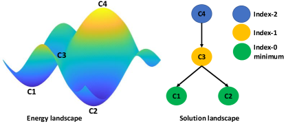
Figure 1: A sketch of an energy landscape and its associated solution landscape ([25]). The $C_{i}$ denote critical points of the energy functional.

Before discussing results, we introduce our nomenclature for labelling critical points. $Stable$ indicates a critical point is stable and therefore index-0. $\pm$ indicates the $Q_{12}$ profile is positive in the interior, whilst $M_{2}$ is negative in the interior. Similarly, $\mp$ means $Q_{12}$ is negative in the interior, whilst $M_{2}$ is positive in the interior, and $+$ $(-)$ means both $Q_{12}$ and $M_{2}$ are positive (negative) in the interior. For unstable saddle points with index greater or equal to 1, we use the following rules. $F$ denotes that we have a full solution which exploits the full four degrees of freedom. Since full solutions come in pairs, we follow $F$ by a number to indicate the pair that we are referring to and finally another number to indicate which solution in the pair we are interested in. For example, $F1.2$ represents solution 2, of full solution pair 1. We denote the unique global energy minimising OR solution for large $l$, by $OR$. This solution branch persists as $l$ decreases, so we continue to denote the solution on this branch by $OR$. We find more OR solutions as $l$ decreases and to identify them we simply enumerate them as $OR1$, $OR2,\ldots$ etc.

III.1 Effects of varying $l$

We begin by taking $c=1$ and varying $l$, to see the impact $l$ has on the connectivity of the solution landscape. We know from [10] Theorem 2.5, that for $l$ sufficiently large ($l>1.25$ approximately when $c=1$), we have a unique OR solution which is the global energy minimiser. This is indeed true and we plot the unique OR solution (labelled as $OR$) for $l=10$ and $c=1$ in Figure 2. This unique solution loses stability for sufficiently small $l$ ([10] Theorem 3.3). Hence, we consider small values of $l$ only in this study.

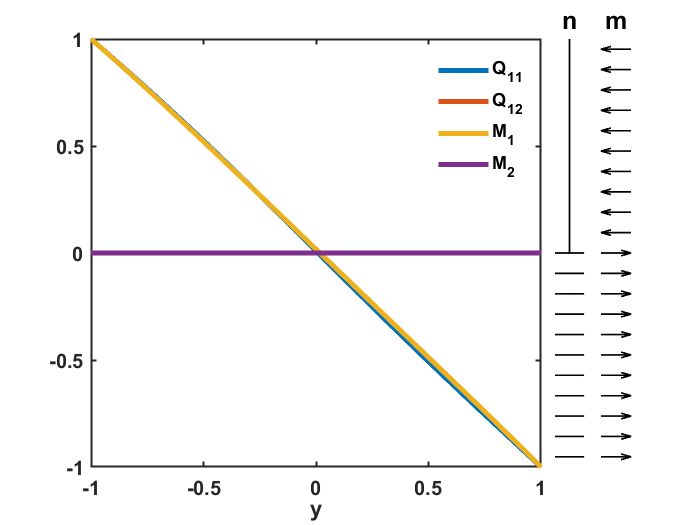
$OR$

Figure 2: The only critical point of (2) for $l=10$ and $c=1$. Note, $Q_{11}=M_{1}=-y$ and $Q_{12}=M_{2}\equiv 0$. Here we plot the components of $\mathbf{Q}$ and $\mathbf{M}$, as well as the associated director profile $\mathbf{n}$, and normalised magnetisation vectors $\mathbf{m}=\mathbf{M}/|\mathbf{M}|$ (we do this for all solutions). $\mathbf{n}$ is plotted as a line field due to the physical equivalence of $\mathbf{n}$ and $-\mathbf{n}$ in the nematic phase [26], while $\mathbf{m}$ is a unit vector and therefore plotted as arrows.

III.1.1 $l=1$ and $c=1$

For $l=c=1$ we find two stable solutions which exploit the full four degrees of freedom, and these are presented in Figure 3. As expected from Remark 1, we have a pair of minimisers for which the $Q_{11}$ and $M_{1}$ profile are the same, whilst the $Q_{12}$ and $M_{2}$ profiles have opposite signs. To be clear, in Figure 3, $Stable+$ and $Stable-$ have the same $Q_{11}$ and $M_{1}$ profile, but the $Q_{12}$ and $M_{2}$ profiles are reflections of one another in the $y$-axis. Letting $\theta$ denote the director angle for $Stable+$, and $\gamma$ the director angle for $Stable-$, it follows that $\theta+\gamma=0$ on $\Omega$. Hence, the director is $\mathbf{n}=(n_{1},n_{2})$ for $Stable+$, and $\mathbf{n}=(n_{1},-n_{2})$ for $Stable-$. The $\mathbf{m}$ profiles for each solution vary in their sense of rotation too, since the $M_{2}$ profiles have opposite signs. This point is also true for all subsequent full solution pairs we present, we therefore do not comment on this again.

Regarding saddle points, we are only able to find one, an index-1 OR solution (presented in Figure 3). This solution is just the continuation of the unique $OR$ solution for large $l$ (i.e., it lies on the same solution branch). The connectivity is therefore simple in this case, $Stable+$ and $Stable-$ are connected via the transition state $OR$ only (see Figure 3). In this case, one can visualise how the pathway evolves by imagining interpolating between $Stable+$ to $OR$, and then $OR$ to $Stable-$, or vice versa. That is, the $Q_{12}$ and $M_{2}$ profiles collapse to zero as $Stable+$ or $Stable-$ approach OR along the pathway, while $Q_{11}$ and $M_{1}$ approach each other, so that $Q_{11}\approx M_{1}$ as in $OR$. This causes the director and magnetisation vector to reorientate from a smooth rotation into a polydomain as we approach $OR$ from $Stable+$ ($Stable-$), which is then reversed with an opposite sense of rotation as we approach $Stable-$ ($Stable+$). These parameter values highlight the importance of OR solutions in switching processes, as in this instance, transition pathways are mediated by an OR solution only.

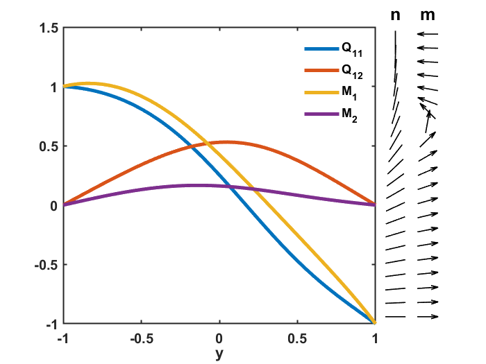
$Stable+$

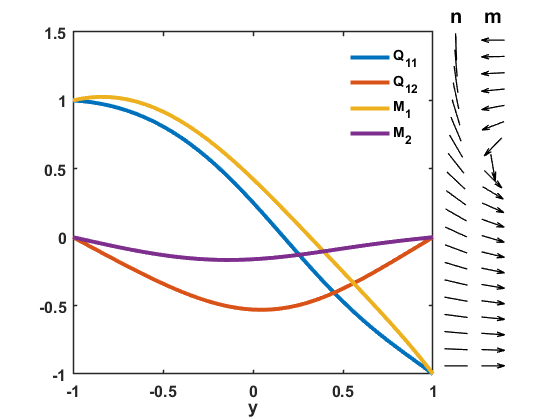
$Stable-$

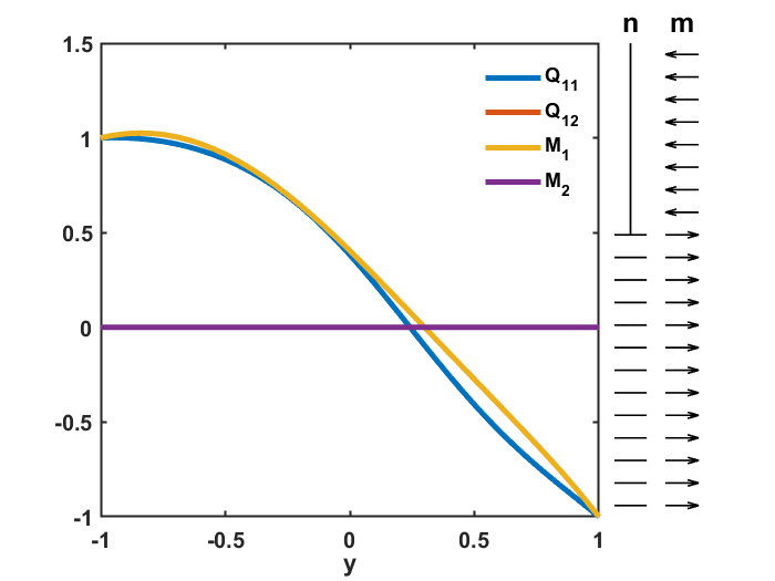
$OR$ - index-1 saddle

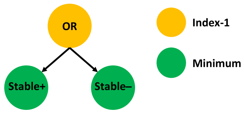
Figure 3: First row: The stable critical points of (2) for $l=1$ and $c=1$. Second row: The only unstable critical point of (2) for $l=1$ and $c=1$ (left) and the solution landscape (right).

III.1.2 $l=0.2$ and $c=1$

For $l=1$ and $c=1$ we find one OR solution which is a transition state. A natural question then, is what is the effect of the parameter $l$ on the index and multiplicity of OR solutions? To partially answer this, we now take $l=0.2$ and $c=1$. We choose this value of $l$, as we only expect to see qualitatively different features in the solution landscape for $l<0.55$, or for $l\ll 0.2$. We know this from the bifurcation diagram in [10]. We keep $c=1$ so we can make comparisons with the $l=1$ case above.

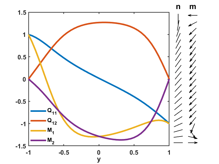
$Stable\pm$

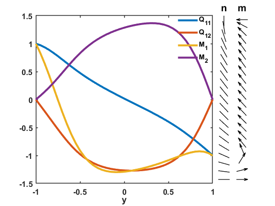
$Stable\mp$

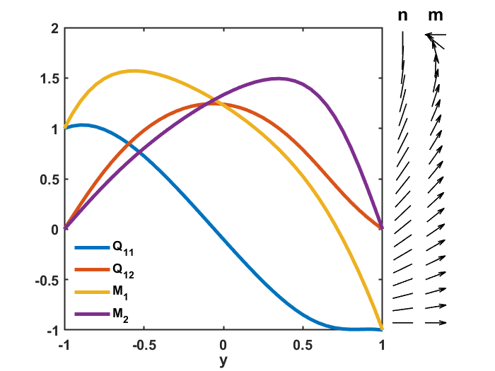
$Stable+$

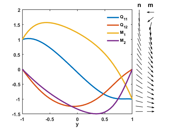
$Stable-$

Figure 4: The stable critical points of (2) for $l=0.2$ and $c=1$.

When $l=0.2$ and $c=1$, the number of stable states of the ferronematic free energy (2) increases to four. We present these states in Figure 4. These four solutions come in two pairs, where once again, the $Q_{11}$ and $M_{1}$ profile are the same in each pair, whilst the $Q_{12}$ and $M_{2}$ profiles are different, in that they have opposite signs. The two pairs are $(Stable+,Stable-)$ and $(Stable\pm,Stable\mp)$.

The number of unstable saddle points of the free energy (2), also increases for $l=0.2$ and $c=1$ when compared to the $l=1$ case. We now have nine saddles and these are presented in Figure 5, along with their indexes. As with the stable full solutions, we see that the unstable full solutions come in pairs and the Morse index of both solutions in the pair is the same. Specifically, the pairs of this form are: $F1.1$ and $F1.2$ (both index-1), $F2.1$ and $F2.2$ (both index-1), and $F3.1$ and $F3.2$ (both index-2). Looking at the director plots for the index-1 pairs $F1$ and $F2$, we see that most of the rotation occurs at either end of the channel. Conversely, for the index-2 pair $F3$, the rotation of $\mathbf{n}$ starts in the channel centre and this maybe why the index is higher. There is no discernible pattern to pick out from the magnetisation vector plots.

As well as these full solutions, we also observe three OR solutions, these are, $OR$ and $OR1$, which are both index-1 saddles, and $OR2$ which is an index-2 saddle. $OR$ is still the continuation of the unique OR solution branch for large $l$, while $OR1$ and $OR2$ are new critical points. We notice that all three OR solutions have one nematic and magnetic domain wall, which do not coincide. Therefore, the likely reason as to why $OR2$ has higher index, is because its magnetic domain wall occurs in the centre of the channel. This is consistent with Theorem 3.2 in [10] and its conclusions. Here the authors analyse the convergence of OR solutions in the limit $l\to 0$. They compute the transition costs between the points $(Q_{11},M_{1})=(\rho^{*},\sqrt{1+2c\rho^{*}}):=\mathbf{p}^{*}$ and $(Q_{11},M_{1})=(\rho^{*},-\sqrt{1+2c\rho^{*}});=\mathbf{p}^{**}$, and find that the energy minimiser (amongst OR solutions) is $\mathbf{p}^{*}$ (with boundary layers to satisfy the boundary conditions at $y=\pm 1$). While $\mathbf{p}^{**}$ has higher energy than $\mathbf{p}^{*}$, it still has lower energy than any solution with internal transition layers in $M_{1}$ (i.e., a solution which jumps between $\mathbf{p}^{*}$ and $\mathbf{p}^{**}$). Expressions of the form $(Q_{11},M_{1})=(\rho^{*},\pm\sqrt{1+2c\rho^{*}})$ define the OR bulk energy density minimisers (i.e., minimisers of the bulk energy when $Q_{12}=M_{2}=0$), where

$$\rho^{*}=\left(\frac{c}{8}+\sqrt{\frac{c^{2}}{64}-\frac{1}{27}\left(1+\frac{c^{2}}{2}\right)^{3}}\right)^{\frac{1}{3}}\\ +\left(\frac{c}{8}-\sqrt{\frac{c^{2}}{64}-\frac{1}{27}\left(1+\frac{c^{2}}{2}\right)^{3}}\right)^{\frac{1}{3}}.$$ (5)

For $c=1$, $\rho^{*}=1.3008$ and $\sqrt{1+2c\rho^{*}}=1.8978$. It follows that $OR$ is approximately equal to $\mathbf{p}^{*}$ in the interior, $OR1$ is approximately equal to $\mathbf{p}^{**}$ in the interior, whilst $OR2$ jumps from $\mathbf{p}^{*}$ to $\mathbf{p}^{**}$, via a transition layer. So, it is highly likely that $OR2$ has higher index because it has an internal transition layer (and central magnetic domain wall due to $M_{1}=0$ at $y\approx-0.17$) which is energetically expensive.

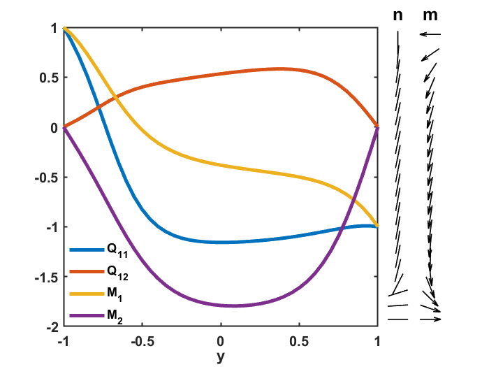
$F1.1$ - index-1 saddle

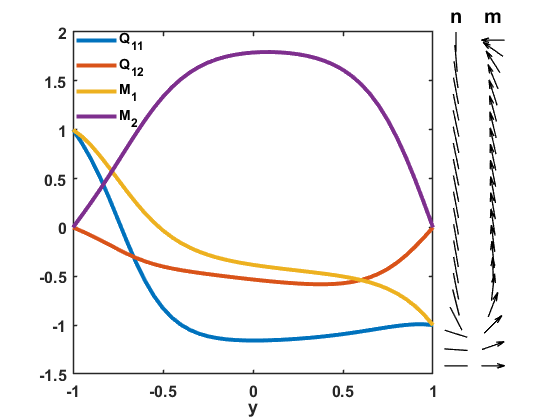
$F1.2$ - index-1 saddle

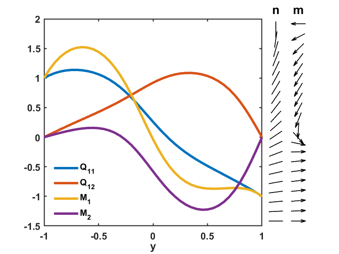
$F2.1$ - index-1 saddle

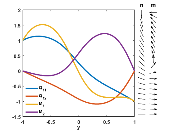
$F2.2$ - index-1 saddle

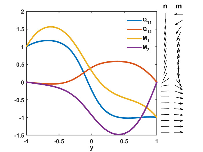
$F3.1$ - index-2 saddle

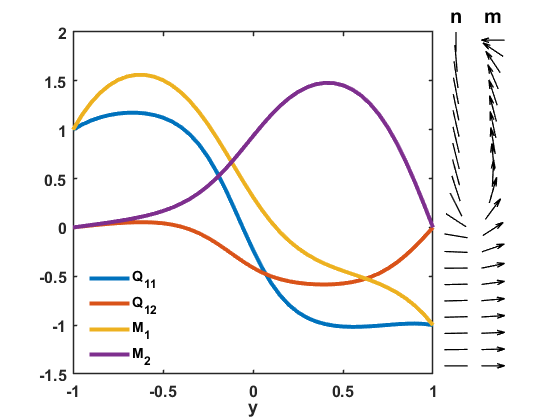
$F3.2$ - index-2 saddle

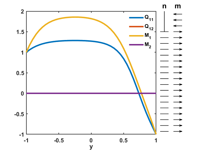
$OR$ - index-1 saddle

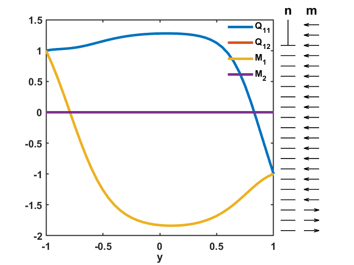
$OR1$ - index-1 saddle

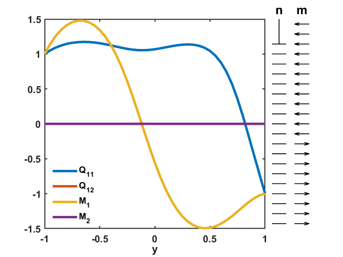
$OR2$ - index-2 saddle

Figure 5: Unstable saddle points of the energy (2) for $l=0.2$ and $c=1$.

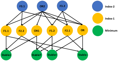
Figure 6: Solution landscape for $l=0.2$ and $c=1$. We only include arrows showing how an index-$i$ state connects to any index-$i+1$ state. That is not to say there do not exist pathways between index-$i$ and index-$i+2$ (or higher) states. We do not include arrows for these pathways since our diagrams become cluttered and difficult to interpret. These comments apply to all subsequent diagrams depicting solution landscapes.

In Figure 6, we report on the connectivity of the solution landscape, that is, how the four stable states in Figure 4, connect to the unstable saddle points in Figure 5. Of particular interest, are the index-1 saddle points that connect stable states, because as mentioned previously, these are transition states which maybe physically observable in switching processes. Each of the stable states can be connected via one of the index-1 full solutions $F1.1$, $F1.2$, $F2.1$, $F2.2$. The OR solutions $OR$ and $OR1$, are also transition states which can connect $Stable\pm$ to $Stable\mp$, and $Stable+$ to $Stable-$, respectively. So again, OR solutions may be important in switching processes for small $l$. The importance of OR solutions does not end there though, since $OR2$ is the parent state (the state with highest index, which connects to all solutions with the next highest index, i.e., $OR2$ connects to all index-1 states in Figure 6). We also find that we can connect any pair of the stable states via $OR2$.

III.1.3 $l=0.1$ and $c=1$

We now take $l=0.1$ and $c=1$, to continue investigating how the index and multiplicity of OR solutions changes with $l$. In view of the results in the previous subsection, we also address this same question for full solutions.

Through the use of Newton’s method and the HiOSD method, we find a total of thirty-nine critical points, these are: seventeen pairs of full solutions and five OR solutions. In terms of stability, we have four stable full solutions, twelve pairs of unstable full solutions and all five OR solutions are unstable. There are three pairs of full solutions we could not find using the HiOSD method, but did find using Newton’s method, hence we cannot comment on their stability. Given the large number of critical points, it is likely we did not find the correct perturbations (see the SI text for details) to obtain these six solutions using the HiOSD method. As such, the solution landscape is incomplete for these parameter values and therefore not presented. We instead plot two new OR solutions in Figure 7, $OR3$ (index-2) and $OR4$ (index-3), both of which have multiple magnetic domain walls. $OR3$ has two internal magnetic domain walls, which is more than any other OR solution we have found, and it is also the highest index OR solution we have found. This again supports the idea that a higher index is associated with a greater number of energetically expensive internal magnetic domain walls. The take away point from this case study with $l=0.1$ and $c=1$, is the sharp increase in the number of critical points, and therefore the increase in complexity of the energy and associated solution landscape. As $l$ decreases we have seen new emergent solutions due to bifurcations. We can expect this to continue as $l$ decreases further, hence a study for $l<0.1$ and $c=1$ such that more bifurcations occur is not practically possible.

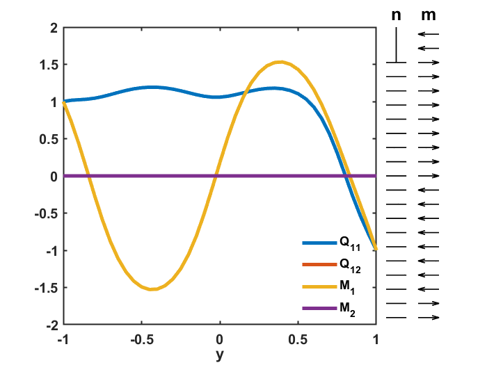
$OR3$ - index-2 saddle

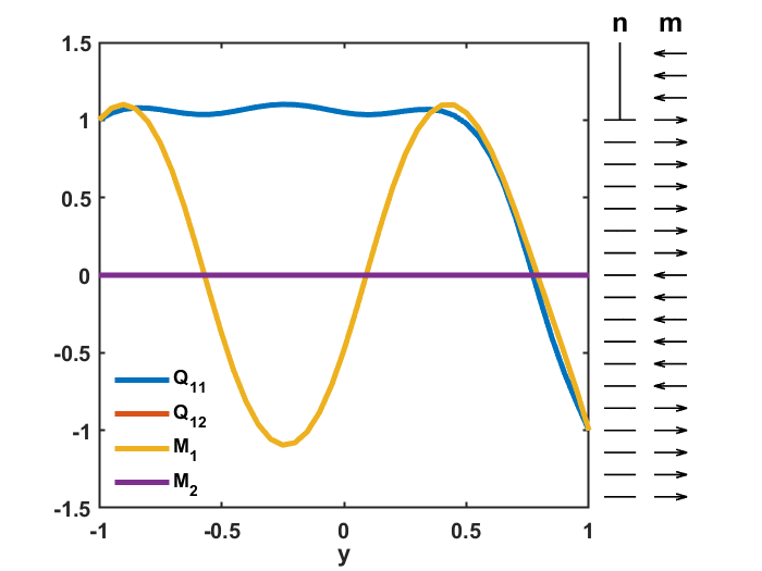
$OR4$ - index-3 saddle

Figure 7: Two unstable OR saddle points of the energy (2) for $l=0.1$ and $c=1$.

III.1.4 Observations and conjectures

We see the total number of critical points increase from $1\to 3\to 13\to 39$, as we decrease $l$ (for $c=1$ fixed) from $10\to 1\to 0.2\to 0.1$. This can be further broken down into how the number of OR and full solutions change. For OR solutions, the multiplicity goes from $1\to 1\to 3\to 5$ as $l$ decreases from $10\to 1\to 0.2\to 0.1$. As for full solutions, the multiplicity increases from $0\to 2\to 10\to 34$, as $l$ decreases from $10\to 1\to 0.2\to 0.1$. A rule which matches this multiplicity sequence, and may therefore predict the number of full solutions at a given bifurcation point, is as follows: the number of full solutions at the $n$’th bifurcation point is given by the formula

$$2+(n-1)\times 2^{(n+1)}.$$ (6)

Using this predicts 98 full solutions at the next bifurcation point (i.e. the fourth). This is likely not the true number of full solutions, but it does give us an approximate idea of the number. We stress that this rule is a conjectures as we have an insufficient number of results to fully validate it. What is certain, is that the number of critical points will increase substantially for an $l<0.1$, such that more bifurcations occur. Indeed, simulating Newton’s method ten thousand times with $l=0.01$ and random initial conditions (see the SI text), we find at least 98 total critical points. Therefore, even a partial understanding of the solution landscape will be difficult to obtain.

III.2 Effects of varying $c$

In [10], they show that increasing $c$ decreases the window of stability of OR solutions. That is, the value $l^{*}(c)$, such that $OR$ is the unique global energy minimiser for $l>l^{*}(c)$, is an increasing function of $c$. Therefore, we hypothesize that solution landscapes with the same qualitative features as those shown in Section III.1, exist for a fixed $l$ and different $c$. To test this, we begin by fixing $l=1$ and vary $c$.

III.2.1 $l=1$ and $c<1$

We start by considering $c<1$, for which we always find two full solutions and no unique OR solution. For $c=0$, $l\geq 1.316$ is needed to achieve a unique OR solution. Hence, this is an approximate lower bound on the value of $l$ required to achieve a unique OR solution (and unique global energy minimiser of (2)), for any value of $c$. With $K=10^{-11}$ and $A=-848.5$Nm^-2 [21], this tells us the maximum channel width for which we can observe a unique OR solution is $1.89\times 10^{-7}$m.

III.2.2 $l=1$ and $c=3$

We take $c=3$ to see whether the number of critical points and/or the solution landscape changes. We find four stable critical points, instead of two, as recorded for $l=c=1$. These can once again be identified as $Stable\pm$, $Stable\mp$, $Stable+$ and $Stable-$. These solutions are visually very similar to those in Figure 4 for $l=c=1$ (the only difference being $|\mathbf{Q}|:=\sqrt{Q_{11}^{2}+Q_{12}^{2}}$ and $|\mathbf{M}|:=\sqrt{M_{1}^{2}+M_{2}^{2}}$ increase in the interior due to the larger value of $c$), so we do not present them. Looking at the unstable saddle points, we now have nine of them, as opposed to one when $l=c=1$. These are six full solutions and three OR solutions all of which can be identified with the same nomenclature as the solutions in Figure 5, since they are continuations of them. Again, there are only minor difference in appearance due to the larger value of $c$, which causes $|\mathbf{Q}|$ and $|\mathbf{M}|$ to increase in the interior, so we omit plots of the solutions. It is worth noting for the OR solutions, that the nematic domain walls move closer to the channel wall at $y=1$, while the magnetic domain walls move closer to $y=1$ if they are in the top half of the channel, and move closer to $y=-1$ if they are in the lower half of the channel.

It is unsurprising then that the solution landscape is qualitatively the same to that shown in Figure 6. By this, we mean for $l=1$ and $c=3$, we have the same number of stable, unstable, full and OR critical points, with the same features, index and connections to one another, as for $l=0.2$ and $c=1$ (henceforth this is what mean by a solution landscape being qualitatively the same). Therefore, we can refer to Figure 6 again to give the solution landscape for $l=1$ and $c=3$. This numerical experiment leads us to believe that the hypothesis at the start of this section is true. For $l=c=1$, and for $l=1$ and $c=3$, we have different solution landscapes, with the latter being equivalent to the solution landscape for $l=0.2$ and $c=1$. This demonstrates that increasing $c$ decreases the effective value of $l$. Looking at the free energy (2), we can see this is because decreasing $l$ and increasing $c$ both increase the dominance of the bulk terms relative to the elastic terms.

III.2.3 $c=5$

So far in this section we have varied $c$ for a fixed $l$. To conclude this section, we now investigate the solution landscape when $c=5$, for different values of $l$. This study is motivated by the bifurcation diagram in [10], which suggest there may be interesting behaviour when both $l$ and $c$ are large. For $l>4.56$, we observe a unique OR solution which we label as $OR$, and this solution persists for smaller values of $l$. We then decrease $l=4.5$ and we immediately observe a new solution landscape. For this value of $l$, a bifurcation has occurred as we now have three OR solutions (see Figure 8), however, no full solutions have emerged. Previously, we have seen a bifurcation away from the unique OR solution by the emergence of a pair of full solutions (see the $l=c=1$ case), and not due to the emergence of new OR solutions. This is interesting, as it means we have identified a parameter regime where we have multiple solutions, all of which are OR solutions. We have two stable OR solutions, $OR$ and $OR1$, which can be connected by and therefore switched between, via the index-1 state $OR2$ (see Figure 9 row 1). Regarding the appearance of the OR solutions in Figure 8, they vary in the location of nematic and magnetic domain walls, but not the multiplicity.

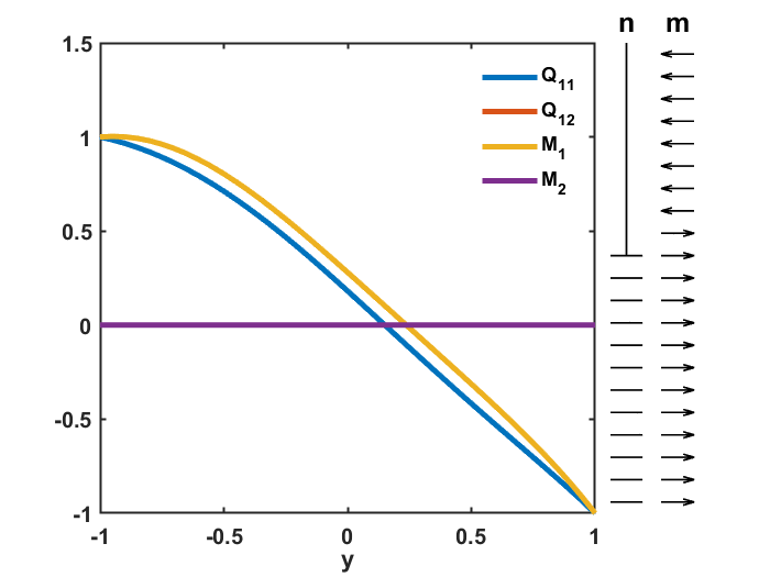
$OR$ - stable

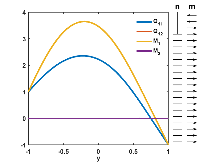
$OR1$ - stable

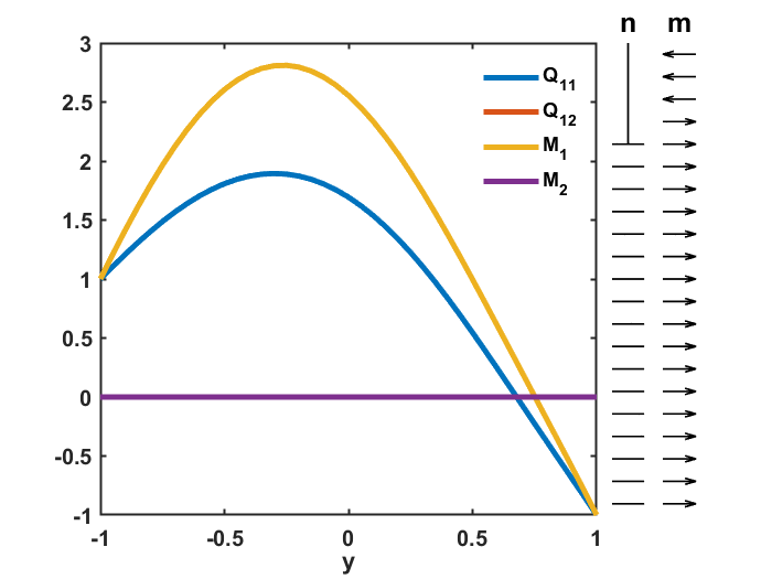
$OR2$ - index-1 saddle

Figure 8: Critical points of the energy (2) for $l=4.5$ and $c=5$.

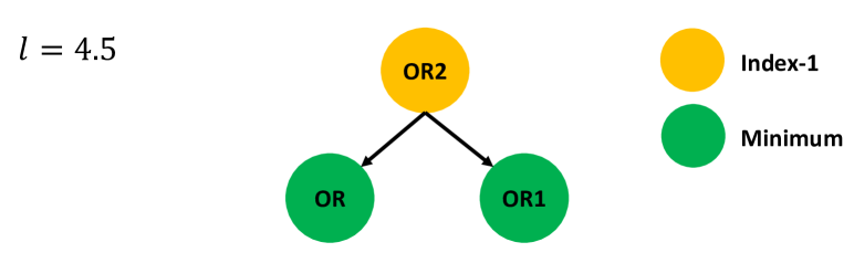
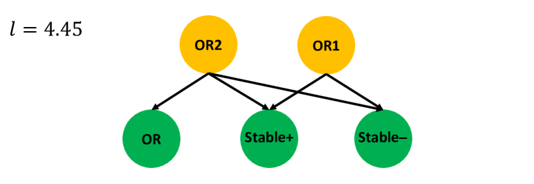
Figure 9: Solution landscapes for $c=5$ and the indicated values of $l$.

We now decrease $l$ further to $l=4.45$, which is accompanied by another bifurcation. We now find two new stable states which are a pair of full solutions that can be categorised as $Stable+$ and $Stable-$, and these are the only new solutions which emerge. The three OR solutions reported in Figure 8 still exist for $l=4.45$. The associated solution landscape is shown in Figure 9 row 2, where we find $OR$ remains stable, $OR2$ remains index-1, and $OR1$ becomes index-1 too. This demonstrates we can have co-stability between OR and full solutions, something not observed in our studies with small $l$ and $c$. We also find $OR2$ to be the parent state. Hence, we can switch between a stable OR solution and stable full solutions, via an OR transition state, making OR solutions doubly important here as they can be stable states and dictate the dynamics/selection of stable states.

We continue to decrease $l$ to see how the multiplicity and importance of OR solutions changes. This is tracked in Figure 11 via a bifurcation diagram. For $l=4.4$ and $c=5$, we have five stable states, the four familiar stable full solutions, and $OR$ which remains stable. So we again have co-stability between OR and full solutions. We find eight other critical points, six of which are new full solutions, while the states $OR1$ and $OR2$ persist and remain index-1 saddles. For $l=4$ and $c=5$ we see that the solution branches for the full solution pairs $F2$ and $F3$, cease to exist and are replaced by two new OR solutions, $OR3$ (index-1) and $OR4$ (index-2 and the new parent state), which emerge for $l\approx 4.35$. These new OR solutions are presented in Figure 10. All other solutions persist from $l=4.4$ and their stability/index is unchanged. We have five OR solutions for these parameter values, making them almost as prevalent as full solutions (there are six). Finally, for $l=3$ and $c=5$ the solution branches for $OR$ and $OR2$, cease to exists (they do not exist for $l>3.6$ approximately). All other solutions persist and their index is unchanged, making $Stable\pm$, $Stable\mp$, $Stable+$ and $Stable-$ the only stable solutions once again. Hence, the key point for these parameter values is the reduction in OR solutions and their importance to the solution landscape. In particular, we no longer have co-stability between OR solutions and full solutions. In summary, this study highlights that large $c$ and large $l$ enhance the formation and importance of OR solutions.

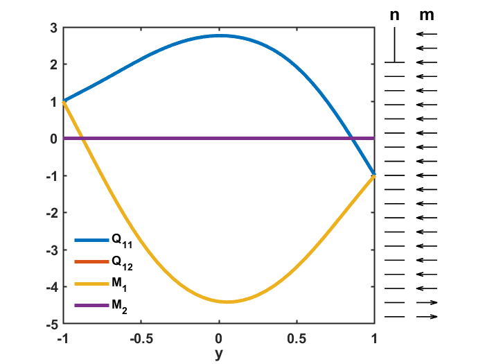
$OR3$ - index-1 saddle

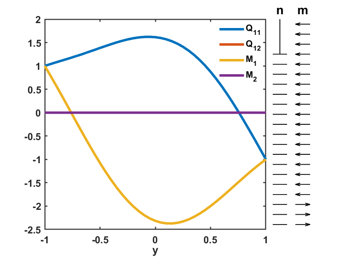
$OR4$ - index-2 saddle

Figure 10: Two unstable OR saddle points of the energy (2) for $l=4$ and $c=5$.

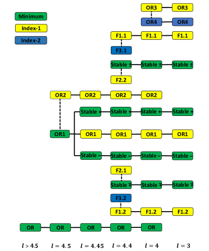
Figure 11: Bifurcation diagram for $c=5$.

III.3 Effects of negative $c$

In [10], and thus far in this paper, only positive $c>0$ is considered. We now study negative $c$ and to draw comparisons with the case of positive $c$, we take $c=-1$ and $l=0.2$. Starting with the stable solutions, we again find four stable full solutions. In fact, we can make a clear correspondence between these stable solutions and those in Figure 4. By reflecting $Q_{11}$ and $M_{1}$ in Figure 4 in the horizontal-axis of the plot, and then reflecting the result in the vertical-axis of the plot, we obtain the $Q_{11}$ and $M_{1}$ profiles for the solutions with $c=-1$. Whilst for $Q_{12}$ and $M_{2}$, reflecting the profiles in Figure 4 in the vertical-axis of the plot, gives the $Q_{12}$ and $M_{2}$ profiles for the solutions with $c=-1$. This means $\mathbf{n}=(-\cos(\theta(-y)),\sin(\theta(-y)))$ and $\mathbf{m}=(-M_{1}(-y),M_{2}(-y))/||\mathbf{M}(-y)||$ for $l=0.2$ and $c=-1$, where $\theta(y)$ and $M_{1}(y)$, $M_{2}(y)$ are the director angle and components of $\mathbf{M}$ respectively, for $l=0.2$ and $c=1$.

Regarding unstable saddle points, like the case of $l=0.2$ and $c=1$, we find nine saddle points, three OR solutions (two index-2 and one index-1) and six full solutions (four index-1 and two index-2). Moreover, the connections we made between the stable solutions for the positive and negative $c$ cases in the previous paragraph, also hold true for these saddle points i.e., they are reflections of those in Figure 5. As such, we can identify them with the same nomenclature as used in Figure 5. There is clearly a connection between all solutions for positive and negative $c$, which we now make precise.

Lemma III.1.

If $(\tilde{Q}_{11},\tilde{Q}_{12},\tilde{M}_{1},\tilde{M}_{2})(y)$ is the solution to the Euler-Lagrange equations (3a)-(3d), subject to the boundary conditions (4), for $c>0$ and $l>0$, then $(-\tilde{Q}_{11},\tilde{Q}_{12},-\tilde{M}_{1},\tilde{M}_{2})(-y)$ is the corresponding solution to (3a)-(3d), subject to the boundary conditions (4), for $-c<0$ and $l>0$.

The proof follows by direct computation and is therefore omitted. It is perhaps unsurprising then, that when we map the solution landscape for $l=0.2$ and $c=-1$, we find it to be qualitatively the same to that when $l=0.2$ and $c=1$. We therefore refer the reader to Figure 5 once again and the subsequent discussion.

III.3.1 Observations and conjectures

In view of Lemma III.1, and the fact that the solution landscapes for $l=0.2$ and $c=\pm 1$ are the same (in terms of the number of stable, unstable, full and OR critical points, their profiles (up to reflections), and their connections), we believe that the for any given $l$ and $c$, the solution landscape for $l$ and $-c$, will be the same. A quick check with $l>1.25$ and $c=-1$ yields a unique OR solution, whilst for $l=1$ and $c=-1$, we recover the solution landscape in Figure 3, giving further support to this claim. Hence, we can refer back to our extensive study on the effects of $l$ and $c$ in Section III.1 and Section III.2, respectively. Differences between the positive and negative $c$ case, should only manifest in the appearance of the actual solutions, and we describe these differences in this section.

IV Conclusions

In this paper, we perform an extensive exploration of solution landscapes of one-dimensional ferronematics for different values of $l$ and $c$, through the implementation of the HiOSD algorithm. This enables us to identify the Morse index of solutions to the Euler-Lagrange equations (3), and track how critical points are connected to one another on the energy landscape for specific choices of $l$ and $c$. Hence, yielding useful information for potential applications in switchable multistable ferronematic devices.

Our results show that fixing $c$ and decreasing $l$, has the same effect on the solution landscape as fixing $l$ and increasing $c$, in that both result in more bifurcations and new emergent solutions. Surprisingly, in some cases, we find repeating solution landscapes for different values of $l$ and $c$. For instance, we observe the solution landscape in Figure 6 for three choices of $(l,c)$, namely $(0.2,1)$, $(1,3)$ and $(0.2,-1)$. As such, we believe there are regions in the $(l,c)$ parameter space where the solution landscapes will be qualitatively the same (i.e., they will have the same number of stable critical points, unstable saddles of a given type and index, along with the same connections between them). We also conclude that as $l$ decreases (for $c$ fixed), or $c$ increases (for $l$ fixed), the index of the parent state increases.

In all of our case studies OR solutions are important to the solution landscape. For those where an OR solution is the parent state, we find these states can mediate pathways between any of the stable states making them eminently useful for switchable devices. We also find OR solutions to be transition states between the $Stable\pm$ and $Stable\mp$ states, and between the $Stable+$ and $Stable-$ states (see Figures 6 and 9). For $c=5$, we even find co-stability between OR solutions and full solutions, so that OR solutions are both a selectable state and states that dictate selection dynamics. In general, pathways mediated by OR solutions are prevalent in all the solution landscapes we investigate. Perhaps our best discovery is for $c=5$ and $l=4.5$, where we find two stable OR solutions, which are connected via an index-1 OR solution, and these are the only critical points. This is a useful and unexpected find, as it illustrates there are parameter regimes for which we can have multistable systems dictated by OR solutions only. Further work would be to identify more parameter values where this occurs.

Finally, we look at negative $c$, which has not previously been considered in this one-dimensional framework. We find the negative $c$ case is entirely equivalent to the positive $c$ case, up to some reflections of the solution profiles. This indicates the results proven in [10], are true for negative $c$ after some minor modifications.

We conclude with an interesting idea worthy of further study. We have seen for $l=0.1$ and $c=1$ we have a large number of solutions to (3) (39 total), and we speculate 98 solutions is an approximate lower bound for the total number of solutions when $l=0.01$ and $c=1$. Ultimately, as $l$ decreases (or equivalently $c$ increases) the behaviour of the system of equations (3) becomes chaotic, due to large increases in the number of critical points for small changes in the parameter values. As such, the usefulness of the model deteriorates for more extreme parameter values. As commented on before, $l=7.37\times 10^{-6}$ is a physically realistic value, but we could not hope to understand the solution landscape in this case. However, a possible solution is as follows. In [27], the authors add stochastic terms to the governing differential equations for nematic liquid crystals confined to a square domain. The idea here, is that the deterministic model is essentially an idealised situation that cannot account for material imperfections, experimental uncertainties or random events, but including stochastic noise can go someway to capturing these effects. Using this approach, they find solutions from the deterministic approach survive qualitatively (i.e., they are perturbed by the noise), but the formation of some solutions are either suppressed or enhanced by the noise. We therefore suggest that the inclusion of noise to this ferronematic problem would lead to a significantly reduced number of qualitatively distinct solutions being observed, e.g. OR solutions with certain polydomain structures or full solutions with a certain sense of rotation for $\mathbf{n}$ and $\mathbf{m}$. This would resolve the chaotic behaviour permitting studies for more physically realistic values of the model parameters.

Numerical solvers

A critical point $(\mathbf{Q},\mathbf{M})$ of (2) is said to be stable if the corresponding Hessian of the free energy $F(\mathbf{Q},\mathbf{M})$ is positive definite, or equivalently, all its eigenvalues are positive, and is unstable otherwise. Here and hereafter, we will denote a critical point by

$$(\mathbf{Q},\mathbf{M}):=(Q_{11},Q_{12},M_{1},M_{2}),$$ (7)

i.e., a single vector containing information about the $\mathbf{Q}$ and $\mathbf{M}$ profiles, in this order. We find solutions of the associated system of Euler-Lagrange equations of (2), (3a)-(3d) in two ways:
 
1. We solve the corresponding gradient flow equations, namely [11]

$$\frac{\partial Q_{11}}{\partial t}=l\frac{\mathrm{d}^{2}Q_{11}}{\mathrm{d}y^{2}}-4Q_{11}(Q_{11}^{2}+Q_{12}^{2}-1)+c\left(M_{1}^{2}-M_{2}^{2}\right),$$ (8a)

$$\frac{\partial Q_{12}}{\partial t}=l\frac{\mathrm{d}^{2}Q_{12}}{\mathrm{d}y^{2}}-4Q_{12}(Q_{11}^{2}+Q_{12}^{2}-1)+2cM_{1}M_{2},$$ (8b)

$$\frac{\partial M_{1}}{\partial t}=l\frac{\mathrm{d}^{2}M_{1}}{\mathrm{d}y^{2}}-M_{1}\left(M_{1}^{2}+M_{2}^{2}-1\right)+2cQ_{11}M_{1}$$

$$\quad\quad\quad\quad\quad\quad\quad\quad\quad\quad\quad\quad+2cQ_{11}M_{1}+2cQ_{12}M_{2},$$ (8c)

$$\frac{\partial M_{2}}{\partial t}=l\frac{\mathrm{d}^{2}M_{2}}{\mathrm{d}y^{2}}-M_{2}\left(M_{1}^{2}+M_{2}^{2}-1\right)$$

$$\quad\quad\quad\quad\quad\quad\quad\quad\quad\quad\quad\quad-2cQ_{11}M_{2}+2cQ_{12}M_{1}.$$ (8d)

To solve the gradient flow system, we use finite difference methods in the space direction with a uniform mesh of mesh size $1/50$ partitioning $[-1,1]$, and use Euler’s method in the time direction.
 
2. Alternatively, we solve the Euler-Lagrange equation (3) using Newton’s method with the same mesh size.
 
Either method is deemed to have converged when the norm of the gradient of $F$ (denoted by $\nabla F$) has fallen below $10^{-8}$, i.e.,

$$||\nabla F(\mathbf{Q},\mathbf{M})||_{L^{2}}<10^{-8},$$ (9)

where

$$\nabla F(\mathbf{Q},\mathbf{M})=\\ \begin{pmatrix}l\frac{\mathrm{d}^{2}Q_{11}}{\mathrm{d}y^{2}}-4Q_{11}(Q_{11}^{2}+Q_{12}^{2}-1)+c\left(M_{1}^{2}-M_{2}^{2}\right)\\ l\frac{\mathrm{d}^{2}Q_{12}}{\mathrm{d}y^{2}}-4Q_{12}(Q_{11}^{2}+Q_{12}^{2}-1)+2cM_{1}M_{2}\\ l\frac{\mathrm{d}^{2}M_{1}}{\mathrm{d}y^{2}}-M_{1}\left(M_{1}^{2}+M_{2}^{2}-1\right)+2cQ_{11}M_{1}+2cQ_{12}M_{2}\\ l\frac{\mathrm{d}^{2}M_{2}}{\mathrm{d}y^{2}}-M_{2}\left(M_{1}^{2}+M_{2}^{2}-1\right)-2cQ_{11}M_{2}+2cQ_{12}M_{1}\end{pmatrix}.$$

We require these two approaches for the following reasons. We couple method 1. with the HiOSD dynamics for eigenvectors (explained next) to compute eigenvalues and eigenvectors of stable critical points. This provides us with suitable initial conditions to start searching the solution landscape using the HiOSD method. We use method 2. to find critical points we may have missed using the HiOSD method. By simulating Newton’s method many times (typically 10000 simulations or more) with random initial conditions (the initial values of $Q_{11},Q_{12}$ and $M_{1},M_{2}$ are generated from a uniform distribution on $[-\rho^{*},\rho^{*}]$ and $[-\sqrt{1+2c\rho^{*}},\sqrt{1+2c\rho^{*}}]$ respectively, where $\rho^{*}$ is defined in the main text), we can in principle find all critical points for given values of the parameters $l$ and $c$, but learn no information about their connections on the energy landscape.

IV.1 The HiOSD method

The Morse index of any critical point is the number of negative eigenvalues of the Hessian of the free energy [23]. Hence, a critical point is unstable if it has Morse index greater or equal to 1 (i.e, it has at least on negative eigenvalue of its Hessian). A saddle point is an unstable critical point which has Morse index-$k$ and hence $k$ negative eigenvalues of the associated Hessian, making it unstable in $k$-distinguished eigendirections and stable in all other directions. Henceforth, we refer to critical points of a given Morse index as index-$k$ saddles. These index-$k$ saddles are non-energy minimising critical points.

For a non-degenerate index-$k$ saddle point $(\hat{\mathbf{Q}},\hat{\mathbf{M}})$, the Hessian $\mathbb{H}(\mathbf{Q},\mathbf{M})=\nabla^{2}F(\mathbf{Q},\mathbf{M})$ at $(\hat{\mathbf{Q}},\hat{\mathbf{M}})$, has exactly $k$ negative eigenvalues $\hat{\lambda}_{1}\leqslant\cdots\leqslant\hat{\lambda}_{k}$ with corresponding unit eigenvectors $\hat{\mathbf{v}}_{1},\ldots,\hat{\mathbf{v}}_{k}$, satisfying $\big{\langle}\hat{\mathbf{v}}_{j},\hat{\mathbf{v}}_{i}\big{\rangle}=\delta_{ij}$, $1\leqslant i,j\leqslant k$. We define a $k$-dimensional subspace $\hat{\mathcal{V}}=\mathrm{span}\big{\{}\hat{\mathbf{v}}_{1},\ldots,\hat{\mathbf{v}}_{k}\big{\}}$, then $(\hat{\mathbf{Q}},\hat{\mathbf{M}})$ is a local maximum on a $k$-dimensional linear manifold $(\hat{\mathbf{Q}},\hat{\mathbf{M}})+\hat{\mathcal{V}}$ and a local minimum on $(\hat{\mathbf{Q}},\hat{\mathbf{M}})+\hat{\mathcal{V}}^{\perp}$, where $\hat{\mathcal{V}}^{\perp}$ is the orthogonal complement space of $\hat{\mathcal{V}}$.

The index-$k$ saddle $(\hat{\mathbf{Q}},\hat{\mathbf{M}})$ can be achieved by a minimax optimization problem

$$\min_{(\mathbf{Q},\mathbf{M})_{\hat{\mathcal{V}}^{\perp}}\in\hat{\mathcal{V}}^{\perp}}\max_{(\mathbf{Q},\mathbf{M})_{\hat{\mathcal{V}}}\in\hat{\mathcal{V}}}F((\mathbf{Q},\mathbf{M})_{\hat{\mathcal{V}}^{\perp}}+(\mathbf{Q},\mathbf{M})_{\hat{\mathcal{V}}}),$$ (10)

where $(\mathbf{Q},\mathbf{M})_{\hat{\mathcal{V}}}=\mathcal{P}_{\hat{\mathcal{V}}}(\mathbf{Q},\mathbf{M})$ is the orthogonal projection of $(\mathbf{Q},\mathbf{M})$ on $\hat{\mathcal{V}}$, and $(\mathbf{Q},\mathbf{M})_{\hat{\mathcal{V}}^{\perp}}=(\mathbf{Q},\mathbf{M})-\mathcal{P}_{\hat{\mathcal{V}}}(\mathbf{Q},\mathbf{M})$. Here, $(\mathbf{Q},\mathbf{M})$ is assumed to be sufficiently close to $(\hat{\mathbf{Q}},\hat{\mathbf{M}})$ so that $\mathbb{H}(\mathbf{Q},\mathbf{M})$ also has exactly $k$ negative eigenvalues, with corresponding eigenvectors $\mathbf{v}_{i}$, for $i=1,\ldots k$. Furthermore, we take $\mathcal{V}=\mathrm{span}\big{\{}\mathbf{v}_{1},\ldots,\mathbf{v}_{k}\big{\}}$ to approximate $\hat{\mathcal{V}}$.

For brevity of notation, in what follows ^. will denote differentiation with respect to $t$. To find a solution of the minimax problem (10), the dynamics of $(\mathbf{Q},\mathbf{M})$ should satisfy that $\mathcal{P}_{\mathcal{V}}(\dot{\mathbf{Q}},\dot{\mathbf{M}})$ is an ascent direction on the subspace $\mathcal{V}$ and that $(\dot{\mathbf{Q}},\dot{\mathbf{M}})-\mathcal{P}_{\mathcal{V}}(\dot{\mathbf{Q}},\dot{\mathbf{M}})$ is a descent direction on the subspace $\mathcal{V}^{\perp}$. This ensures $(\mathbf{Q},\mathbf{M})$ increases to a maximum on $\mathcal{V}$ and decreases to a minimum on $\mathcal{V}^{\perp}$. Therefore, we take $\mathcal{P}_{\mathcal{V}}\nabla F(\mathbf{Q},\mathbf{M})$ as the direction of $\mathcal{P}_{\mathcal{V}}(\dot{\mathbf{Q}},\dot{\mathbf{M}})$ and $-\nabla F(\mathbf{Q},\mathbf{M})+\mathcal{P}_{\mathcal{V}}\nabla F(\mathbf{Q},\mathbf{M})$ as the direction of $(\dot{\mathbf{Q}},\dot{\mathbf{M}})-\mathcal{P}_{\mathcal{V}}(\dot{\mathbf{Q}},\dot{\mathbf{M}})$. The following gradient dynamics can then be used to solve (10)

$$\beta^{-1}(\dot{\mathbf{Q}},\dot{\mathbf{M}})=-\nabla F(\mathbf{Q},\mathbf{M})+2\mathcal{P}_{\mathcal{V}}\nabla F(\mathbf{Q},\mathbf{M}),$$ (11)

where $\beta>0$ is a relaxation parameter.

The $k$-dimensional subspace $\mathcal{V}$ is constructed by solving the following constrained optimization problem

$$\min_{\mathbf{v}_{i}\in\mathbb{R}^{n}}\;\langle\mathbb{H}(\mathbf{Q},\mathbf{M})\mathbf{v}_{i},\mathbf{v}_{i}\rangle,\;\mathrm{s.t.}\;\langle\mathbf{v}_{j},\mathbf{v}_{i}\rangle=\delta_{ij},\;j=1,2,\ldots,i.$$ (12)

Using the simultaneous Rayleigh-quotient iterative minimisation method [28] to solve (12), and noting that under the orthonormal constraint, $\mathcal{P}_{\mathcal{V}}$ is given by $\Sigma_{i=1}^{k}\mathbf{v}_{i}\mathbf{v}_{i}^{\top}$, we obtain a dynamical system of the HiOSD for finding an index-$k$ saddle point,

$$\left\{\begin{aligned} &\beta^{-1}(\dot{\mathbf{Q}},\dot{\mathbf{M}})=-\left(\mathbf{I}-2\sum_{j=1}^{k}\mathbf{v}_{j}\mathbf{v}_{j}^{\top}\right)\nabla F(\mathbf{Q},\mathbf{M}),\\ &\gamma^{-1}\dot{\mathbf{v}}_{i}=-\left(\mathbf{I}-\mathbf{v}_{i}\mathbf{v}_{i}^{\top}-2\sum_{j=1}^{i-1}\mathbf{v}_{j}\mathbf{v}_{j}^{\top}\right)\mathbb{H}(\mathbf{Q},\mathbf{M})\mathbf{v}_{i},\;\\ &\qquad\qquad\qquad\qquad\qquad\qquad\qquad\qquad\textrm{for }i=1,\ldots,k,\end{aligned}\right.$$ (13)

where the state variable $(\mathbf{Q},\mathbf{M})$ and $k$ direction variables $\mathbf{v}_{i}$ are coupled, $\mathbf{I}$ is the identity operator and $\gamma>0$ is a relaxation parameter.

We implement Algorithm 1 in [14], with the following choices to solve this dynamical system. We take our relaxation parameters $\beta=\gamma=\Delta t$, where $\Delta t$ is our Euler time step size used to solve the gradient flow equations (8a)-(8d). Furthermore, we fix $l^{0}=10^{-6}$ and deem the method to have converged when $||\nabla F(\mathbf{Q},\mathbf{M})||_{L^{2}}<10^{-8}$. An input into this algorithm is a solution of the gradient flow equations (8a)-(8d), along with its orthonormal eigenvectors $\mathbf{v}_{i}$, where $i=1,\ldots,n$ and $n\in\mathbf{N}$. To find the $\mathbf{v}_{i}$, we take $n$ random orthonormal vectors as our initial condition and simultaneously iterate the dynamics for $\mathbf{v}_{i}$ in (13), as we solve the gradient flow equations. Our initial condition for the method is then a perturbation of the form $(\mathbf{Q},\mathbf{M})+\epsilon\mathbf{v}_{i}$, where we take $\epsilon\in(0,1]$. In principle any eigendirection $\mathbf{v}_{i}$ is possible, but it is typically sufficient to check the first few eigendirections (starting from the eigenvector with the smallest eigenvalue). To find an index-$k$ saddle, we choose $k\in\mathbb{Z}^{+}$ (such that $k\leq n$) as our final input to Algorithm 1 in [14]. An index-$k$ saddle found using this initial condition is connected to the state $(\mathbf{Q},\mathbf{M})$, or equivalently there is a pathway between them. Once an index-$k$ saddle and its eigenvectors have been found, we can use this state to construct new initial conditions and repeat the process just outlined to find higher, or lower index saddles and deduce their connectivity.

References

- de Gennes. and Prost [1993] P. G. de Gennes. and J. Prost, The Physics of Liquid Crystals, 2nd ed. (Clarendon Press, Oxford, 1993).
- Stewart [2004] I. W. Stewart, The Static and Dynamic Continuum Theory of Liquid Crystals: A Mathematical Introduction (Taylor & Francis, London and New York, 2004).
- Gartland et al. [2010] E. Gartland, H. Huang, O. Lavrentovich, P. Palffy-Muhoray, I. Smalyukh, T. Kosa, and B. Taheri, Electric-field induced transitions in a cholesteric liquid-crystal film with negative dielectric anisotropy, J. Comput. Theor. Nanosci. 7, 709 (2010).
- Lagerwall and Scalia [2012] J. P. F. Lagerwall and G. Scalia, A new era for liquid crystal research: Applications of liquid crystals in soft matter nano-, bio- and microtechnology, Current Applied Physics 12, 1387 (2012).
- Brochard and de Gennes [1970] F. Brochard and P. G. de Gennes, Theory of magnetic suspensions in liquid crystals, Journal de Physique 31, 691 (1970).
- Burylov and Raikher [1995] S. V. Burylov and Y. L. Raikher, Macroscopic Properties of Ferronematics Caused by Orientational Interactions on the Particle Surfaces. I. Extended Continuum Model, Molecular Crystals and Liquid Crystals 258, 107 (1995).
- Liu et al. [2016] Q. Liu, P. J. Ackerman, T. C. Lubensky, and I. I. Smalyukh, Biaxial ferromagnetic liquid crystal colloids, Proc. Natl. Acad. Sci. 113, 10479 (2016).
- Mertelj et al. [2013] A. Mertelj, D. Lisjak, M. Drofenik, and M. Čopič, Ferromagnetism in suspensions of magnetic platelets in liquid crystals, Nature 504, 237 (2013).
- Jones and Beldon [2004] J. C. Jones and S. Beldon, High Image-Content Zenithal Bistable Devices, SID International Symposium Digest of technical papers 35, 140 (2004).
- Dalby et al. [2022a] J. Dalby, P. Farrell, A. Majumdar, and J. Xia, One-Dimensional Ferronematics in a Channel: Order Reconstruction, Bifurcations and Multistability, SIAM Journal on Applied Mathematics 82, 694 (2022a).
- Bisht et al. [2019] K. Bisht, V. Banerjee, P. Milewski, and A. Majumdar, Magnetic nanoparticles in a nematic channel: a one-dimensional study, Physical Review E 100, 012703 (2019).
- Bisht et al. [2020] K. Bisht, Y. Wang, V. Banerjee, and A. Majumdar, Tailored morphologies in two-dimensional ferronematic wells, Physical Review E 101, 022706 (2020).
- Maity et al. [2021] R. R. Maity, A. Majumdar, and N. Nataraj, Parameter dependent finite element analysis for ferronematics solutions, Computers & mathematics with applications 103, 127 (2021).
- Yin et al. [2019] J. Yin, L. Zhang, and P. Zhang, High-index optimization-based shrinking dimer method for finding high-index saddle points, SIAM Journal on Scientific Computing 41, A3576 (2019).
- Kusumaatmaja and Majumdar [2015] H. Kusumaatmaja and A. Majumdar, Free energy pathways of a multistable liquid crystal device, Soft matter 11, 4809 (2015).
- Han et al. [2021a] Y. Han, J. Yin, P. Zhang, A. Majumdar, and L. Zhang, Solution landscape of a reduced Landau-de Gennes model on a hexagon, Nonlinearity 34, 2048 (2021a).
- Han et al. [2022] Y. Han, J. Dalby, A. Majumdar, B. M. G. D. Carter, and T. Machon, Uniaxial versus biaxial pathways in one-dimensional cholesteric liquid crystals, Physical Review Research 4, L032018 (2022).
- Agha and Bahr [2018] H. Agha and C. Bahr, Nematic line defects in microfluidic channels: wedge, twist and zigzag disclinations, Soft Matter 14, 653 (2018).
- Dalby et al. [2022b] J. Dalby, Y. Han, A. Majumdar, and L. Mrad, A multi-faceted study of nematic order reconstruction in microfluidic channels, arXiv:2204.07808 [math.AP] (2022b).
- Han et al. [2021b] Y. Han, J. Harris, J. Walton, and A. Majumdar, Tailored nematic and magnetization profiles on two-dimensional polygons, Physical Review E 103, 052702 (2021b).
- Luo et al. [2012] C. Luo, A. Majumdar, and R. Erban, Multistability in planar liquid crystal wells, Physical Review E 85, 061702 (2012).
- Majumdar and Zarnescu [2010] A. Majumdar and A. Zarnescu, Landau-de Gennes theory of nematic liquid crystals: the Oseen–Frank limit and beyond, Archive for Rational Mechanics and Analysis 196, 227– (2010).
- Milnor [1963] J. Milnor, Morse Theory, 1st ed. (Princeton University Press, Princeton, NJ, 1963).
- Zhang et al. [2016] L. Zhang, Q. Du, and Z. Zheng, Optimization-based shrinking dimer method for finding transition states, SIAM Journal on Scientific Computing 38, A528 (2016).
- Yin et al. [2020] J. Yin, Y. Wang, J. Z. Y. Chen, P. Zhang, and L. Zhang, Construction of a Pathway Map on a Complicated Energy Landscape, Physical Review Letters 124, 090601 (2020).
- Ball et al. [2017] J. M. Ball, E. Feireisl, and F. Otto, Mathematical Thermodynamics of Complex Fluids: Cetraro, Italy 2015, 1st ed. (Springer International Publishing, Cham, 2017).
- Dalby et al. [2023] J. Dalby, A. Majumdar, Y. Wue, and A. K. Dond, Stochastic effects on solution landscapes for nematic liquid crystals, arXiv:2308.07045 [cond-mat.soft] (2023).
- Longsine and McCormick [1980] D. E. Longsine and S. F. McCormick, Simultaneous rayleigh-quotient minimization methods for , Linear Algebra and its Applications 34, 195 (1980).