Addendum: models for gaps $g=2p_{1}$

Fred B. Holt fbholt62@gmail.com; https://www.primegaps.info
(Date: 25 Sept 2023)
Abstract.

This is an addendum to previous work on the models of populations and relative populations of small gaps $g$ across stages of Eratosthenes sieve. If we have the initial conditions in the cycle of gaps ${\mathcal{G}}({p_{0}}^{\#})$, we can exhibit exact population models for all gaps $g<2p_{1}$. For gaps beyond this threshold $2p_{1}$, we could not be certain of the counts of the driving terms for a gap $g$ of various lengths.

Here we extend this work by introducing the exact population models for $g=2p_{1}$. We are able to get this one additional case in a general form. Using the initial conditions from ${\mathcal{G}}({p_{0}}^{\#})$ we advance the model one time to obtain exact counts for the driving terms for $g=2p_{1}$ in ${\mathcal{G}}({p_{1}}^{\#})$. This iteration uses a different system matrix than the usual one. After this special iteration we can apply the usual dynamics to obtain the exact population model for the gap $g=2p_{1}$ across all stages of Eratosthenes sieve.

Key words and phrases:
primes, gaps, prime constellations, Eratosthenes sieve
1991 Mathematics Subject Classification:
11N05, 11A41, 11A07

1. Setting

This is an addendum to previous work [1, 2] on exact models for the populations and relative populations of gaps $g$ across stages of Eratosthenes sieve. At each stage of Eratosthenes sieve, there is a cycle of gaps ${\mathcal{G}}({p}^{\#})$ of length $\phi({p}^{\#})$ (number of gaps in the cycle) and span ${p}^{\#}$ (sum of the gaps in the cycle).

For example, the cycle ${\mathcal{G}}({5}^{\#})$ has length (number of gaps) $\phi({5}^{\#})=8$ and span (sum of gaps) ${5}^{\#}=30$.

$${\mathcal{G}}({5}^{\#})\makebox[14.45377pt]{}=\makebox[14.45377pt]{}6\;4\;2\;4\;2\;4\;6\;2.$$

There is a recursion from one cycle ${\mathcal{G}}({p_{k}}^{\#})$ to the next ${\mathcal{G}}({p_{k+1}}^{\#})$. We concatenate $p_{k+1}$ copies of ${\mathcal{G}}({p_{k}}^{\#})$ and then add adjacent gaps at the running sums given by the elementwise product $p_{k+1}\ast{\mathcal{G}}({p_{k}}^{\#})$. These additions of adjacent gaps are called fusions. The gaps that survive the fusions are the gaps between primes.

The recursion across the cycles of gaps ${\mathcal{G}}({p_{k}}^{\#})$ is a discrete dynamic system. If we take initial conditions from ${\mathcal{G}}({p_{0}}^{\#})$, then we can create exact population models for all gaps $g<2p_{1}$. The populations all grow superexponentially, so we divide by factors of $p_{k}-2$ to obtain the exact models for relative populations for all gaps $g<2p_{1}$.

$\displaystyle w_{g}({p_{k+1}}^{\#})\;=\;\left[\begin{array}[]{c}w_{g,1}\\ w_{g,2}\\ \vdots\\ w_{g,J}\end{array}\right]_{{p_{k+1}}^{\#}}$ $\displaystyle=$ $\displaystyle\left[\begin{array}[]{ccccc}1&\scriptstyle\frac{1}{p_{k+1}-2}&0&\cdots&0\\ 0&\scriptstyle\frac{p_{k+1}-3}{p_{k+1}-2}&\scriptstyle\frac{2}{p_{k+1}-2}&&0\\ 0&0&\scriptstyle\frac{p_{k+1}-4}{p_{k+1}-2}&\ddots&0\\ \vdots&\vdots&\ddots&\ddots&\vdots\\ 0&0&\cdots&\cdots&\scriptstyle\frac{p_{k+1}-J-1}{p_{k+1}-2}\end{array}\right]\cdot\left[\begin{array}[]{c}w_{g,1}\\ w_{g,2}\\ \vdots\\ w_{g,J}\end{array}\right]_{{p_{k}}^{\#}}$
$\displaystyle=$ $\displaystyle M_{J}(p_{k+1})\cdot w_{g}({p_{k}}^{\#})$
$\displaystyle=$ $\displaystyle M_{J}^{k+1}\cdot w_{g}({p_{0}}^{\#})$

Here the elements $w_{g,j}$ denote the relative population of driving terms for gap $g$ of length $j$. $w_{g,1}({p}^{\#})$ is the relative population of the gap $g$ itself in the cycle ${\mathcal{G}}({p}^{\#})$. And we use the notation $M^{k}$ to denote the product of matrices:

$$M_{J}^{k}\;=\;M_{J}(p_{k})\cdot M_{J}(p_{k-1})\cdots M_{J}(p_{2})\cdot M_{J}(p_{1})$$

$w_{g}({p_{0}}^{\#})$ is the vector of the initial conditions in the cycle of gaps ${\mathcal{G}}({p_{0}}^{\#})$. These are the counts of the gap $g$ in this cycle and of all of its driving terms, divided by the population of gaps $2$. We need $J$ to be at least as large as the longest driving terms for $g$.

For more details about the discrete dynamic system and the population models, please see the prior work [1, 2].

2. Models for $g<2p_{1}$

The iterative model

$$w_{g}({p_{k}}^{\#})\;=\;M_{J}^{k}w_{g}({p_{0}}^{\#})$$

only applies to gaps $g<2p_{1}$.

This constraint $g<2p_{1}$ arises from needing to be sure that under the recursion each fusion occurs in its own copy of a driving term for $g$. This allows us to get the exact counts across driving terms of all lengths. Since the fusions are spaced according to the elementwise product $p_{k+1}\ast{\mathcal{G}}({p_{k}}^{\#})$ and the smallest element in ${\mathcal{G}}({p_{k}}^{\#})$ is $2$, the fusions are separated by at least $2p_{k}$. So $g<2p_{0}$ suffices to use the iterative system for the gap $g$.

The challenge to us developing models for larger gaps $g$ is that we need to get the initial populations from a cycle of gaps ${\mathcal{G}}({p_{0}}^{\#})$ such that $g<2p_{1}$. The cycle ${\mathcal{G}}({p}^{\#})$ has length $\phi({p}^{\#})$.

$p$ $29$ $31$ $37$ $41$ $43$ $47$ $53$ $59$
$\max g$ $60$ $72$ $80$ $84$ $92$ $104$ $116$ $120$
$\phi({p}^{\#})$ $\scriptstyle 1.02E9$ $\scriptstyle 3..07E10$ $\scriptstyle 1.10E12$ $\scriptstyle 4.41E13$ $\scriptstyle 1.85E15$ $\scriptstyle 8.53E16$ $\scriptstyle 4.44E18$ $\scriptstyle 2.57E20$

We see that computing ${\mathcal{G}}({59}^{\#})$ is at the horizon of current computing capability, and this would enable us to calculate the initial conditions for the models for all gaps $g\leq 120$.

For the models in our prior work [1, 2] we used ${\mathcal{G}}({37}^{\#})$ and exhibited the relative population models for $g\leq 80$.

3. Models for $g=2p_{1}$

We can extend the models to cover the case $g=2p_{1}$. The important insight here is that the populations of driving terms for this gap $g$ can be exactly produced from the initial conditions $w_{g}({p_{0}}^{\#})$. We have to use a different system matrix to update the relative populations for $g$ and its driving terms from $w_{g}({p_{0}}^{\#})$ to $w_{g}({p_{1}}^{\#})$. After this one special iteration we can apply the general model described above.

The special first iteration is motivated by the following Lemma.

Lemma 3.1.

Let $s$ be a constellation of span $g$ in ${\mathcal{G}}({p_{k}}^{\#})$. If $p_{k+1}|g$, then both ends of $s$ are fused in the same copy under the recursion from ${\mathcal{G}}({p_{k}}^{\#})$ to ${\mathcal{G}}({p_{k+1}}^{\#})$.

This is Lemma 28 on page 139 of [2]

Let $s$ be a driving term for $g$ of length $j$. Under the recursion from ${\mathcal{G}}({p_{0}}^{\#})$ to ${\mathcal{G}}({p_{1}}^{\#})$, the concatenation step initially produces $p_{1}$ copies of $s$. Each of the possible $j+1$ fusions in $s$ will occur exactly once. The $j-1$ interior fusions will result in a shorter driving term for $g$ in ${\mathcal{G}}({p_{1}}^{\#})$, and the $2$ boundary fusions will eliminate that image of $s$ as a driving term for $g$.

In order to get a count of the driving terms for $g=2p_{1}$ in ${\mathcal{G}}({p_{1}}^{\#})$, we need to confirm that the $j-2$ interior fusions occur in separate images of $s$, and that the $2$ boundary fusions eliminate only $1$ image of $s$.

For any interior fusion in $s$, the span from this fusion to either end of $s$ is strictly less than $2p_{1}$. But the smallest distance between spans is $2p_{1}$, and thus the interior fusions will occur in separate images of $s$. The interior fusions in $s$ result in $j-1$ driving terms for $g$ of length $j-1$.

By the lemma above, the two boundary fusions occur in the same image of $s$, eliminating exactly one image of $s$ as a driving term for $g$. Note that this is specific to $g=2p_{1}$; for $g<2p_{1}$ the two boundary fusions occur in separate images of $s$.

So for the gap $g=2p_{1}$, each driving term $s$ of length $j$ in ${\mathcal{G}}({p_{0}}^{\#})$ produces $j-1$ driving terms of length $j-1$ in ${\mathcal{G}}({p_{1}}^{\#})$, one image of $s$ is removed as a driving term for $g$, and $p_{1}-j$ images of $s$ are preserved intact as driving terms for $g$ in ${\mathcal{G}}({p_{1}}^{\#})$. This specific iteration for $w_{g=2p_{1}}$ is

$\displaystyle w_{g}({p_{1}}^{\#})$ $\displaystyle=$ $\displaystyle\widehat{M}_{J}(p_{1})\cdot w_{g}({p_{0}}^{\#})$
$\displaystyle=$ $\displaystyle\left[\begin{array}[]{cccccc}\scriptstyle\frac{p_{1}-1}{p_{1}-2}&\scriptstyle\frac{1}{p_{1}-2}&0&0&\cdots&0\\ 0&1&\scriptstyle\frac{2}{p_{1}-2}&0&&0\\ 0&0&\scriptstyle\frac{p_{1}-3}{p_{1}-2}&\scriptstyle\frac{3}{p_{1}-2}&\ddots&0\\ \vdots&\vdots&\ddots&\ddots&\ddots&\vdots\\ 0&0&0&0&\cdots&\scriptstyle\frac{p_{1}-J}{p_{1}-2}\end{array}\right]\cdot w_{g}({p_{0}}^{\#})$

If we have computed the cycle ${\mathcal{G}}({p_{0}}^{\#})$ for initial conditions, the counts of the driving terms across a range of gaps $g$, we normalize these counts by the number of gaps $2$ and from these relative populations $w_{g}({p_{0}}^{\#})$ we have the complete exact models for the relative populations across all subsequent stages of Eratosthenes sieve:

$$w_{g}({p_{k}}^{\#})\;=\;\left\{\begin{array}[]{cc}M_{J}(p_{k})\cdot M_{J}(p_{k-1})\cdots M_{J}(p_{2})\cdot M_{J}(p_{1})\cdot w_{g}({p_{0}}^{\#})&{\rm if}\;g<2p_{1}\\[8.5359pt] M_{J}(p_{k})\cdot M_{J}(p_{k-1})\cdots M_{J}(p_{2})\cdot\widehat{M}_{J}(p_{1})\cdot w_{g}({p_{0}}^{\#})&{\rm if}\;g=2p_{1}\end{array}\right.$$

Specifically, from our initial conditions from ${\mathcal{G}}({37}^{\#})$ we have previously been able to exhibit the population models for all gaps $g\leq 80$. Here $p_{0}=37$ and $p_{1}=41$. We can now add one more model, the model for $g=82$.

To harmonize the collection of models $w_{g}$ for $g\leq 82$, we need the same starting point $p_{0}$. We could use the dynamic system to advance the models for all of the $g\leq 80$ up to $w_{g}({41}^{\#})$ and use $p_{0}=41$ as the starting point; or we could back $w_{82}({41}^{\#})$ up using $M^{-1}_{J}(41)$ to obtain an equivalent surrogate starting point $\widehat{w}_{82}({37}^{\#})$ that provides the exact model $w_{82}({p}^{\#})$ for all $p\geq 41$.

We pursue this second approach here.

$\displaystyle\widehat{w}_{82}({37}^{\#})$ $\displaystyle=$ $\displaystyle M^{-1}_{J}(41)\cdot w_{82}({41}^{\#})$
$\displaystyle=$ $\displaystyle M^{-1}_{J}(41)\cdot\widehat{M}_{J}(41)\cdot w_{82}({37}^{\#})$

This gives us a starting point $\widehat{w}_{82}({37}^{\#})$ that aligns with our other starting points in ${\mathcal{G}}({37}^{\#})$ and that provides the exact values for $w_{82}({p_{k}}^{\#})$ for all $p_{k}\geq 41$. This surrogate starting point $\widehat{w}_{82}({37}^{\#})$ is not the correct relative population $w_{82}({37}^{\#})$.

$\displaystyle\widehat{w}_{82}({37}^{\#})$ $\displaystyle\neq$ $\displaystyle w_{82}({37}^{\#})$
$\displaystyle M_{J}(41)\cdot\widehat{w}_{82}({37}^{\#})$ $\displaystyle=$ $\displaystyle w_{82}({41}^{\#})\;=\;\widehat{M}_{J}(41)\cdot w_{82}({37}^{\#})$

Using ${\mathcal{G}}({37}^{\#})$ for the starting point, we have driving terms for $g=82$ up to length $J=19$. The number of gaps $g=2$ in ${\mathcal{G}}({37}^{\#})$ is

$$n_{2,1}({37}^{\#})=217929355875.$$

For the gap $g=82$ we tabulate the data from ${\mathcal{G}}({37}^{\#})$. Our calculations have some numerical errors on the order of $10^{-13}$.

$j$ $n_{82,j}({37}^{\#})$ $w_{82,j}({37}^{\#})$ $w_{82,j}({41}^{\#})$ $\widehat{w}_{82,j}({37}^{\#})$ $l_{82,j}$
$1$ $\scriptstyle 0$ $\scriptstyle 0$ $\scriptstyle 0$ $\scriptstyle-2.768491E-13$ $\scriptstyle 1.025641$
$2$ $\scriptstyle 0$ $\scriptstyle 0$ $\scriptstyle 2.353150E-13$ $\scriptstyle 1.976531E-12$ $\scriptstyle 11.553942$
$3$ $\scriptstyle 1$ $\scriptstyle 4.5886429E-12$ $\scriptstyle 1.160809E-09$ $\scriptstyle-3.035074E-12$ $\scriptstyle 60.410483$
$4$ $\scriptstyle 3276$ $\scriptstyle 1.5032394E-08$ $\scriptstyle 1.415302E-07$ $\scriptstyle 1.503443E-08$ $\scriptstyle 194.488465$
$5$ $\scriptstyle 270422$ $\scriptstyle 1.2408700E-06$ $\scriptstyle 5.882215E-06$ $\scriptstyle 1.244637E-06$ $\scriptstyle 431.258857$
$6$ $\scriptstyle 8051838$ $\scriptstyle 3.6947010E-05$ $\scriptstyle 1.179125E-04$ $\scriptstyle 3.716878E-05$ $\scriptstyle 697.937481$
$7$ $\scriptstyle 120058788$ $\scriptstyle 5.5090691E-04$ $\scriptstyle 1.326320E-03$ $\scriptstyle 5.558081E-04$ $\scriptstyle 852.214506$
$8$ $\scriptstyle 1027245782$ $\scriptstyle 4.7136641E-03$ $\scriptstyle 9.081749E-03$ $\scriptstyle 4.769260E-03$ $\scriptstyle 800.382107$
$9$ $\scriptstyle 5411112020$ $\scriptstyle 2.4829661E-02$ $\scriptstyle 3.968207E-02$ $\scriptstyle 2.519649E-02$ $\scriptstyle 584.027075$
$10$ $\scriptstyle 18234669494$ $\scriptstyle 8.3672387E-02$ $\scriptstyle 1.136091E-01$ $\scriptstyle 8.516773E-02$ $\scriptstyle 332.122850$
$11$ $\scriptstyle 40031677310$ $\scriptstyle 1.8369107E-01$ $\scriptstyle 2.155096E-01$ $\scriptstyle 1.875723E-01$ $\scriptstyle 146.758457$
$12$ $\scriptstyle 57338080360$ $\scriptstyle 2.6310398E-01$ $\scriptstyle 2.702203E-01$ $\scriptstyle 2.695709E-01$ $\scriptstyle 49.939794$
$13$ $\scriptstyle 52822037198$ $\scriptstyle 2.4238147E-01$ $\scriptstyle 2.204693E-01$ $\scriptstyle 2.492174E-01$ $\scriptstyle 12.883935$
$14$ $\scriptstyle 30369623454$ $\scriptstyle 1.3935536E-01$ $\scriptstyle 1.135898E-01$ $\scriptstyle 1.438024E-01$ $\scriptstyle 2.461383$
$15$ $\scriptstyle 10389093440$ $\scriptstyle 4.7671840E-02$ $\scriptstyle 3.526600E-02$ $\scriptstyle 4.936702E-02$ $\scriptstyle 0.336767$
$16$ $\scriptstyle 1974527214$ $\scriptstyle 9.0604004E-03$ $\scriptstyle 6.171214E-03$ $\scriptstyle 9.413221E-03$ $\scriptstyle 0.031541$
$17$ $\scriptstyle 192967582$ $\scriptstyle 8.8545933E-04$ $\scriptstyle 5.642306E-04$ $\scriptstyle 9.225035E-04$ $\scriptstyle 0.001910$
$18$ $\scriptstyle 9665424$ $\scriptstyle 4.4351180E-05$ $\scriptstyle 2.673245E-05$ $\scriptstyle 4.631847E-05$ $\scriptstyle 0.000070$
$19$ $\scriptstyle 272272$ $\scriptstyle 1.2493590E-06$ $\scriptstyle 7.047666E-07$ $\scriptstyle 1.308852E-06$ $\scriptstyle 0.000001$
sum $\scriptstyle 217929355875$ $\scriptstyle 1.000000$ $\scriptstyle 1.025641$ $\scriptstyle 1.025641$
Table 1. Data for the gap $g=82$ from the cycle ${\mathcal{G}}({37}^{\#})$. The column $n_{82,j}$ lists the populations of driving terms for $g=82$ for various lengths $j$. The longest driving term has length $J=19$. The column $w_{82,j}({37}^{\#})$ contains the normalized populations for these driving terms, and $w_{82,j}({41}^{\#})$ calculates the relative populations for the driving terms in ${\mathcal{G}}({41}^{\#})$ using $\widehat{M}_{19}(41)$. The next column $\widehat{w}_{82,j}({37}^{\#})$ is the pre-image of $w_{82,j}({41}^{\#})$ under $M^{-1}_{19}(41)$. The final column lists the coefficients $l_{82,j}$ for the population model.

The models update the relative populations of all of the driving terms for $g=82$. If we take just the top row we extract the model just for the relative population of the gap $g=82$ itself.

$$w_{82,1}({p_{k}}^{\#})=\;l_{82,1}-l_{82,2}\prod_{41}^{p_{k}}\frac{q-3}{q-2}+l_{82,3}\prod_{41}^{p_{k}}\frac{q-4}{q-2}-\cdots+l_{82,19}\prod_{41}^{p_{k}}\frac{q-20}{q-2}$$

for all $p_{k}\geq 41$. Table 1 lists these coefficients $l_{82,j}$ in the final column.

4. Notes on models for slightly larger $g$

The beauty of the work above is that we can work directly with the relative populations of driving terms of various lengths $j$. Can we extend these methods any further, to extract models for $g=2p_{1}+2$ or $g=2p_{1}+4$? To do so, we would need to track subpopulations among the driving terms.

Refer to caption
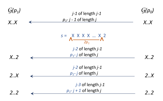
Figure 1. A diagram of the specific iteration for gaps $g=2p_{1}+2$ from ${\mathcal{G}}({p_{0}}^{\#})$ to ${\mathcal{G}}({p_{1}}^{\#})$. ’X’ denotes any gap in a driving term $s$ for $g$ that is not a $2$. If the driving term $s$ does not begin or end with a $2$, then the general model applies. If $s$ ends with a $2$, then that interior fusion occurs in the same image of $s$ as the far boundary fusion. One fewer image of length $j-1$ survives, and one more image of length $j$ survives.

Gaps $g=2p_{1}+2$. This gap is small enough that $g<2p_{2}$, so the only spans that complicate our tracking the counts of the driving terms for $g$ are the spans of $2p_{1}$ where the two fusions occur as a boundary fusion and interior fusion in a single image of a driving term $s$. This will occur iff the driving term $s$ begins or ends with a $2$.

If we separate the counts for the driving terms for $g=2p_{1}+2$ to cover four subpopulations, we could perform a distinct iteration from $w_{2p_{1}+2}({p_{0}}^{\#})$ to $w_{2p_{1}+2}({p_{1}}^{\#})$, after which we can use the general model.

Consider a driving term $s$ for $g$ of length $j$ in ${\mathcal{G}}({p_{0}}^{\#})$. Since $g=2p_{1}+2$ the two boundary fusions occur in different images of $s$, so $p_{1}-2$ images of $s$ survive as driving terms for $g$ in ${\mathcal{G}}({p_{1}}^{\#})$. We need to track their lengths. If the first or last gap in $s$ is a $2$, then by the lemma this interior fusion occurs in the same image of $s$ as the far boundary fusion.

We have the following four subpopulations of driving terms $s$ of span $2p_{1}+2$ and length $j$ in ${\mathcal{G}}({p_{0}}^{\#})$:

  1. (a)

    $s=X\ldots X$. If $s$ begins and ends with gaps other than $2$, then all of the fusions - interior and boundary - occur in separate images of $s$ during the recursive construction of ${\mathcal{G}}({p_{1}}^{\#})$. We can use the general model for these populations described above.

  2. (b)

    $s=X\ldots 2$. If $s$ ends with a $2$, then the interior fusion for this last gap will occur in the same image of $s$ as the boundary fusion at the start of $s$. Of the $p_{1}$ images of $s$ created during the concatenation step, two are eliminated as driving terms for $g$ by the boundary fusions. The one boundary fusion takes an interior fusion along with it. The remaining $j-2$ interior fusions result in driving terms for $g$ in ${\mathcal{G}}({p_{1}}^{\#})$ of length $j-1$. $p_{1}-j$ images of $s$ survive intact as driving terms of length $j$ for $g$ in ${\mathcal{G}}({p_{1}}^{\#})$.

  3. (c)

    $s=2\ldots X$. The cycle of gaps ${\mathcal{G}}({p}^{\#})$ is symmetric. So if $s$ starts with a $2$, the analysis is the same as the previous case.

  4. (d)

    $s=2\ldots 2$. For driving terms $s$ that begin and end with a $2$, these would fall into both of the previous cases, complicating the counts. So we separate them out as their own subpopulation. In this case both boundary fusions coincide with an interior fusion. Of the $j-1$ interior fusions, $j-3$ produce driving terms for $g$ in ${\mathcal{G}}({p_{1}}^{\#})$ of length $j-1$. $p_{1}-j+1$ images of $s$ survive intact as driving terms of length $j$ for $g$ in ${\mathcal{G}}({p_{1}}^{\#})$.

We could exhibit the block banded matrices for this system. But unless we partition the population of driving terms for the gap $g=2p_{1}+2$ into the required subpopulations, we cannot apply this model.

Gaps $g=2p_{1}+4$. For gaps $g=2p_{1}+4$, the subpopulations of driving terms become more complicated. We need to consider cases in which a driving term begins or ends with a $4$, and the analysis parallels the work above for $g=2p_{1}+2$.

We also have to consider the possibility that $g=2p_{2}$, which would occur when $p_{2}=p_{1}+2$.

5. Conclusion

This work serves as an addendum to the existing references [1, 2]. We do not duplicate that background here, beyond summarizing a few needed results.

We have shown previously that at each stage of Eratosthenes sieve there is a corresponding cycle of gaps ${\mathcal{G}}({p}^{\#})$. We can view these cycles of gaps as a discrete dynamic system, and from this system we can obtain exact models for the populations and relative populations of gaps $g<2p_{1}$ if we can get the initial conditions from ${\mathcal{G}}({p_{0}}^{\#})$.

In this addendum we have shown that we can produce the model for ${g=2p_{1}}$ from these initial conditions. This model requires one special iteration to track the count from ${\mathcal{G}}({p_{0}}^{\#})$ to ${\mathcal{G}}({p_{1}}^{\#})$, after which we can use the general model for these populations.

We have further shown that in order to produce the models for ${g=2p_{1}+2}$ and beyond from initial conditions in ${\mathcal{G}}({p_{0}}^{\#})$, we would have to track subpopulations of the driving terms $s$ until the general model applies, that is until ${g<2p_{k+1}}$.

References

  • [1] F.B. Holt, Combinatorics of the gaps between primes, Connections in Discrete Mathematics, Simon Fraser U., arXiv 1510.00743, June 2015.
  • [2] F.B. Holt, Patterns among the Primes, KDP, June 2022.