An analysis of the derivative-free loss method for solving PDEs

Abstract

This study analyzes the derivative-free loss method to solve a certain class of elliptic PDEs using neural networks. The derivative-free loss method uses the Feynman-Kac formulation, incorporating stochastic walkers and their corresponding average values. We investigate the effect of the time interval related to the Feynman-Kac formulation and the walker size in the context of computational efficiency, trainability, and sampling errors. Our analysis shows that the training loss bias is proportional to the time interval and the spatial gradient of the neural network while inversely proportional to the walker size. We also show that the time interval must be sufficiently long to train the network. These analytic results tell that we can choose the walker size as small as possible based on the optimal lower bound of the time interval. We also provide numerical tests supporting our analysis.

MSC codes. 65N15, 65N75, 65C05, 60G46

1 Introduction

The neural network is well known for its flexibility to represent complicated functions in a high-dimensional space [3, 9]. In recent years, this strong property of the neural network has naturally led to representing the solution of partial differential equations (PDEs). Physics-informed neural network [16] and Deep Galerkin [17] use the strong form of the PDE to define the training loss, while the Deep Ritz [4] method uses a weak (or variational) formulation of PDEs to train the network. Also, a class of methods uses a stochastic representation of PDEs to train the neural network [5, 8]. All these methods have shown successful results in a wide range of problems in science and engineering, particularly for high-dimensional problems where the standard numerical PDE methods have limitations [5, 17, 2].

The goal of the current study is an analysis of the derivative-free loss method (DFLM; [8]). DFLM employs a stochastic representation of the solution for a certain class of PDEs, averaging stochastic samples as a generalized Feynman-Kac formulation. The loss formulation of DFLM directly guides a neural network to learn the point-to-neighborhood relationships of the solution. DFLM adopts bootstrapping in the context of reinforcement learning, where the neural network’s target function is computed based on its current state through the point-to-neighborhood relation. This iterative process incrementally refines the neural network toward solving the PDE.

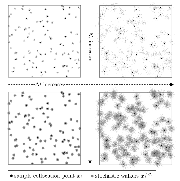
Figure 1: Sampling diagram for DFLM

It is shown in [8] that the derivative-free formulation offers advantages in handling singularities that arise due to the geometric characteristics of the domain, particularly in cases involving sharp boundaries. Also, using the intrinsic averaging character in representing the solution, DFLM has been successfully applied to the homogenization problem [7] and a nonlinear flow problem [14].

As in the other methods to solve PDEs numerically, there are collocation points in DFLM to impose constraints for the solution to satisfy. Additionally, there are $N_{s}$ walkers centered at each collocation point, which is related to the expected value calculation of the Feynman-Kac formula. By solving a certain stochastic process related to the given PDE operator for some time $\Delta t$, DFLM uses an expected value related to the walkers to represent the PDE solution at each collocation point. Note that $\Delta t$ is not the time step to solve a time-dependent problem; we consider only elliptic problems in the current study. Figure 1 shows schematics of DFLM for the two parameters $N_{s}$ and $\Delta t$ of various values. As $N_{s}$ increases (that is, we have more walkers to explore a neighborhood), we have more sample values related to the expectation. In contrast, a large $\Delta t$ increases the spread of the walkers around each collocation point.

A large $N_{s}$ will decrease the sampling error while a long $\Delta t$ will cover a wide range of neighborhoods. However, a large $N_{s}$ and a long $\Delta t$ will increase the overall computational cost; a large $N_{s}$ requires more walkers to run (or more samples to draw using $\tilde{q}$-martingale in Section 2), and $\Delta t$ requires a more extended time period to run the walkers. Our analysis (Theorem 1 in Section 3) shows that the empirical training loss has a bias bounded by $\frac{\Delta t}{N_{s}}$. This result implies that we can use a small $N_{s}$ for computational efficiency while keeping $\Delta t$ small accordingly. In this study, we also show (Theorem 2 in Section 3) that the time interval $\Delta t$ must be sufficiently large to guarantee the training of the PDE solution. When $\Delta t$ is too small, the walkers do not move enough to explore neighborhoods and thus cannot see the local variations of the solution. The overall message of our analysis for DFLM is that there exists an optimal lower bound for the time interval $\Delta t$, and we can choose the number of walkers $N_{s}$ (at a collocation point) as small as possible based on the optimal $\Delta t$.

The current paper is structured as follows. In Section 2, we review DFLM for an elliptic problem, explaining all parameters related to our analysis. Section 3 has all our analytic results for DFLM, including the upper bound of the training loss bias and the training issue using a small $\Delta t$ for the stochastic walkers. We provide numerical examples in Section 4, supporting our analysis. This paper concludes in Section 5 with discussions about limitations and future directions.

2 Derivative-Free Neural Network Training Method

This section reviews the derivative-free loss method (DFLM) for solving a certain type of elliptic PDEs [8]. DFLM tackles the PDEs through the underlying stochastic representation in the spirit of the Feynman-Kac formula that describes how the solution at a point interrelates to its neighborhood. DFLM guides a neural network directly to satisfy the interrelation across the entire domain, leading to the solution of the PDE. This intercorrelation characteristic makes DFLM different from other methods that use pointwise residuals of the strong form PDE, such as PINN [16], in which a neural network implicitly learns the interrelation among different points. Moreover, DFLM gradually and alternately updates a neural network and corresponding target values toward the PDE solution in the same manner as bootstrapping in the context of reinforcement learning, which differs from supervised learning methods that optimize neural network parameters within a fixed topology defined by loss functions.

In this paper, we consider DFLM for the following type of elliptic PDEs of an unknown function $u(\bm{x})\in\mathbb{R}$:

$$\mathcal{N}[u](\bm{x}):=\frac{1}{2}\Delta u(\bm{x})+\bm{V}\cdot\nabla_{\bm{x}}u(\bm{x})-G=0,~{}\textrm{in}~{}\Omega\subset\mathbb{R}^{k}.$$ (1)

Here $\bm{V}=\bm{V}(\bm{x},u(\bm{x}))\in\mathbb{R}^{k}$ is the advection velocity and $G=G(\bm{x},u(\bm{x}))\in\mathbb{R}$ is the force term, both of which can depend on $u$.

From the standard application of It$\hat{\text{o}}$’s lemma (e.g., in [11]), we have the stochastic representation of the solution of Eq. (1) through the following equivalence;

• $u:\Omega\rightarrow\mathbb{R}$ is a solution of Eq. (1).

• the stochastic process $q(t;u,\bm{x},\{\bm{X}_{s}\}_{0\leq s\leq t})\in\mathbb{R}$ defined as

  $$q(t;u,\bm{x},\{\bm{X}_{s}\}_{0\leq s\leq t}):=u(\bm{X}_{t})-\int_{0}^{t}G(\bm{X}_{s},u(\bm{X}_{s}))ds,\\$$ (2)

  where $\bm{X}_{t}\in\mathbb{R}^{k}$ is a stochastic process of the following SDE

  $$d\bm{X}_{t}=\bm{V}(\bm{X}_{t},u(\bm{X}_{t}))dt+d\bm{B}_{t},\quad\bm{B}_{t}:\mbox{ standard Brownian motion in }\mathbb{R}^{k},$$ (3)

  satisfies the martingale property

  $$\begin{split}u(\bm{x})&=q(0;u,\bm{x},\bm{X}_{0})=\mathbb{E}\left[q\left(t;u,\bm{x},\{\bm{X}_{s}\}_{0\leq s\leq t}\right)|\bm{X}_{0}=\bm{x}\right]\\ &=\mathbb{E}\left[u(\bm{X}_{t})-\int_{0}^{t}G(\bm{X}_{s},u(\bm{X}_{s}))ds\middle|\bm{X}_{0}=\bm{x}\right],~{}\forall\bm{x}\in\Omega,\forall t>0.\end{split}$$ (4)

Regarding to the definition of stochastic process $q(t;u,\bm{x},\{\bm{X}_{s}\}_{0\leq s\leq t})$, the infinitesimal drift $d(\cdot)$ of the stochastic process $u(\bm{X}_{t})$ is connected to the differential operator $\mathcal{N}[u]$ as

$$d(u(\bm{X}_{t}))=\left(\mathcal{N}[u](\bm{X}_{t})+G(\bm{X}_{t},u(\bm{X}_{t})\right)dt+\nabla u(\bm{X}_{t})\cdot d\bm{B}_{t}.$$ (5)

The martingale property, Eq. (4), shows that the solution at a point $\bm{x}$, $u(\bm{X})$ can be represented through its neighborhood statistics observed by the stochastic process $\bm{X}_{t}$ starting at the point $\bm{x}$ during the time period $[0,t]$. We note that the representation holds for an arbitrary time $t>0$ and any stopping time $\tau$ by the optional stopping theorem [11]. In particular, the exit time from the domain as the stopping time, $\tau=\inf\{s:\bm{X}_{s}\notin\Omega\}$, induces the well-known Feynman-Kac formula for the PDE [13]. Note that other methods are based on the classical Monte-Carlo of the Feynman-Kac formula [1, 10, 15, 18]. Such methods estimate the solution of a PDE at an individual point independently with the realizations of the stochastic processes $\bm{X}_{t}$ until it exits from the given domain. DFLM, on the other hand, approximates the PDE solution over the domain at once through a neural network $u(\bm{x};\bm{\theta})$, which is trained to satisfy the martingale property Eq. (4). In particular, DFLM considers a short period, say $\Delta t$, rather than waiting for whole complete trajectories until $\bm{X}_{t}$ is out of the domain. This character of DFLM allows a neural network to learn more frequently for a short time period.

DFLM constructs the loss function for training a neural network as

$$\mathcal{L}^{\Omega}(\bm{\theta}) =\mathbb{E}_{\bm{x}\sim\Omega}\left[\left|u(\bm{x};\bm{\theta})-\mathbb{E}\left[q\left(\Delta t;u(\cdot;\bm{\theta}),\bm{x},\{\bm{X}_{s}\}_{0\leq s\leq\Delta t}\right)|\bm{X}_{0}=\bm{x}\right]\right|^{2}\right]$$ (6)

$$=\mathbb{E}_{\bm{x}\sim\Omega}\left[\left|u(\bm{x};\bm{\theta})-\mathbb{E}_{\{\bm{X}_{s}\}_{0\leq s\leq\Delta t}}\left[u(\bm{X}_{t};\bm{\theta})-\int_{0}^{\Delta t}G(\bm{X}_{s},u(\bm{X}_{s};\bm{\theta}))ds\middle|\bm{X}_{0}=\bm{x}\right]\right|^{2}\right]$$ (7)

where the outer expection is over the sample collocation point $\bm{x}$ in the domain $\Omega$ and the inner expectation is over the stochastic path $\bm{X}_{t}$ starting at $\bm{X}_{0}=\bm{x}$ during $[0,\Delta t]$. In the presence of the drive term $\bm{V}$ that can depend on $u$, the statistics of $\bm{V}$ will be nontrivial and thus a numerical approximation to $\bm{X}_{t}$ must be calculated by solving Eq. (3). As an alternative to avoid the calculation of the solution to Eq. (3), another martingale process $\tilde{q}(t;u,\bm{x},\{\bm{B}_{s}\}_{0\leq s\leq t})$ based on the standard Brownian motion $\bm{B}_{t}$ is proposed as

$$\tilde{q}(t;u,\bm{x} ,\{\bm{B}_{s}\}_{0\leq s\leq t}):=\left(u(\bm{B}_{t})-\int_{0}^{t}G(\bm{B}_{s},u(\bm{B}_{s}))ds\right)\mathcal{D}(\bm{V},u,t),$$ (8)

$$\text{where}{\quad}\mathcal{D}(\bm{V},u,t)=\exp\biggl{(}\int^{t}_{0}\bm{V}(\bm{B}_{s},u(\bm{B}_{s}))\cdot d\bm{B}_{s}-\frac{1}{2}\int^{t}_{0}|\bm{V}(\bm{B}_{s},u(\bm{B}_{s}))|^{2}ds\biggr{)}.$$

Here, $\tilde{q}$-process is of form replacing the $\bm{X}_{t}$ to $\bm{B}_{t}$ in $q$-process with additional exponential factor $\mathcal{D}(\bm{V},u,t)$ compensating the removal of the drift effect in $\bm{X}_{t}$ [11, 13]. Using the alternative $\tilde{q}$-martingale allows the standard Brownian walkers to explore the domain regardless of the form of the given PDE, which can be drawn from the standard Gaussian distribution without solving SDEs. The alternative loss function corresponding to $\tilde{q}$-martingale is

$$\mathcal{L}^{\Omega}(\bm{\theta})=\mathbb{E}_{\bm{x}\sim\Omega}\left[\left|u(\bm{x};\bm{\theta})-\mathbb{E}\left[\tilde{q}(t;u(\cdot;\bm{\theta}),\bm{x},\{\bm{B}_{s}\}_{0\leq s\leq\Delta t})|\bm{B}_{0}=\bm{x}\right]\right|^{2}\right].$$ (9)

In the standard DFLM [8], for the Dirichlet boundary condition, $u(\bm{x})=g(\bm{x})$ on $\partial\Omega$, we consider $\bm{X}_{t}$ to be absorbed to the boundary $\partial\Omega$ at the exit position and the value of the neural network is replaced by the given boundary value at the exit position, which makes the information propagate from the boundary into the domain’s interior. In this study, to enhance the constraint on the boundary, we add the following boundary loss term

$$\mathcal{L}^{\partial\Omega}(\bm{\theta})=\mathbb{E}_{\bm{x}\sim\partial\Omega}\left[|u(\bm{x};\bm{\theta})-g(\bm{x})|^{2}\right]$$ (10)

in the total loss

$${\mathcal{L}}(\bm{\theta})={\mathcal{L}}^{\Omega}(\bm{\theta})+{\mathcal{L}}^{\partial\Omega}(\bm{\theta}).$$ (11)

The loss function ${\mathcal{L}}(\bm{\theta})$ is optimized by a stochastic gradient descent method, and, in particular, the bootstrapping approach is used as the target of the neural network (i.e., the expectation component of $q$- or $\tilde{q}$-process) is pre-evaluated using the current state of neural network parameters $\bm{\theta}$. The $n$-th iteration step for updating the parameters $\bm{\theta}_{n}$ is

$$\bm{\theta}_{n}=\bm{\theta}_{n-1}-\alpha\nabla\widetilde{\mathcal{L}}_{n}(\bm{\theta}_{n-1}),{\quad}\text{where}{\quad}\widetilde{\mathcal{L}}_{n}(\bm{\theta})=\widetilde{\mathcal{L}}_{n}^{\Omega}(\bm{\theta})+\widetilde{\mathcal{L}}^{\partial\Omega}(\bm{\theta}).$$ (12)

Here, the term $\widetilde{\mathcal{L}}_{n}^{\Omega}(\bm{\theta})$ is the empirical interior loss function using $N_{r}$ sample collocation points $\{\bm{x}_{i}\}_{i=1}^{N_{r}}$ in the interior of the domain $\Omega$, and $N_{s}$ stochastic walkers $\left\{\bm{X}_{s}^{(i,j)};s\in[0,\Delta t],\bm{X}_{0}=\bm{x}_{i}\right\}_{j=1}^{N_{s}}$ at each sample collocation point $\bm{x}_{i}$,

$$\widetilde{\mathcal{L}}^{\Omega}_{n}(\bm{\theta}): =\widetilde{\mathbb{E}}_{\bm{x}\sim\Omega}\left[\left|u(\bm{x};\bm{\theta})-\widetilde{\mathbb{E}}\left[q\left(\Delta t;u(\cdot;\bm{\theta}_{n-1}),\bm{x},\{\bm{X}_{s}\}_{0\leq s\leq\Delta t}\right)|\bm{X}_{0}=\bm{x}\right]\right|^{2}\right]$$ (13)

$$=\frac{1}{N_{r}}\sum\limits_{i=1}^{N_{r}}\left|u(\bm{x}_{i};\bm{\theta})-\frac{1}{N_{s}}\sum\limits_{j=1}^{N_{s}}\left\{u\left(\bm{X}_{\Delta t}^{(i,j)};\bm{\theta}_{n-1}\right)-\int_{0}^{\Delta t}G\left(\bm{X}_{s}^{(i,j)},u\left(\bm{X}_{\Delta t}^{(i,j)};\bm{\theta}_{n-1}\right)\right)ds\right\}\right|^{2}.$$ (14)

The other term $\widetilde{\mathcal{L}}^{\partial\Omega}(\bm{\theta})$ is the empirical boundary loss function using $N_{b}$ random boundary collocation points $\{\bm{x}_{l}\}_{l=1}^{N_{b}}$ on $\partial\Omega$

$$\widetilde{\mathcal{L}}^{\partial\Omega}(\bm{\theta}):=\widetilde{\mathbb{E}}_{\bm{x}\sim\partial\Omega}\left[|u(\bm{x};\bm{\theta})-g(\bm{x})|^{2}\right]=\frac{1}{N_{b}}\sum\limits_{l=1}^{N_{b}}\left|u(\bm{x}_{l};\bm{\theta})-g(\bm{x}_{l})\right|^{2}.$$ (15)

The random interior and boundary collocation points $\{\bm{x}_{i}\}_{i=1}^{N_{r}}$ and $\{\bm{x}_{l}\}_{l=1}^{N_{b}}$ can follow a distribution whose support covers the domain $\Omega$ and the boundary $\partial\Omega$, respectively. The learning rate $\alpha$ could be tuned at each step and the gradient descent step can be optimized by considering the previous steps, such as Adam optimization [12].

3 Analysis

DFLM utilizes stochastic walkers within each local neighborhood of collocation points over the domain. Our primary interest is to comprehend these stochastic walkers’ influence on the training of a neural network. The information integrated into the neural network during each iteration is affected by two key parameters: i) the time interval $\Delta t$ and ii) the number of stochastic walkers $N_{s}$. Both parameters determine how far (by $\Delta t$) and densely (by $N_{s}$) the walkers collect the information around the corresponding collocation points (see Fig. 1). We show in this section that the network’s training to approximate a PDE solution is hindered by the bias of the empirical loss function, which depends on the two parameters. Moreover, we show that DFLM requires suitably spacious neighborhood observations through the stochastic walkers to approximate the solution effectively. This implies that a lower bound $\Delta t^{\ast}$ exists for the time interval $\Delta t$.

3.1 Bias in the empirical martingale loss function

Theorem 1.

The empirical loss $\widetilde{\mathcal{L}}^{\Omega}(\bm{\theta})$ in Eq. (13) is a biased estimator of the exact martingale loss $\mathcal{L}^{\Omega}(\bm{\theta})$ in Eq. (6). Moreover, when $u(\cdot;\bm{\theta})$ has a small PDE residual $\mathcal{N}[u(\cdot;\bm{\theta})]$ in Eq. (1), the bias is proprotional to $\Delta t$ and the $\mathcal{L}^{2}$-norm of $\nabla_{\bm{x}}u(\cdot;\bm{\theta})$ with respect to the sampling measure $\bm{x}\sim\Omega$, while the bias is inversely proportional to $N_{s}$

$${\mbox{Bias}}_{\mathcal{L}^{\Omega}}\left[\widetilde{\mathcal{L}}^{\Omega}\right]{\quad}\propto{\quad}\frac{\Delta t}{N_{s}}\mathbb{E}_{\bm{x}\sim\Omega}\left[|\nabla_{\bm{x}}u(\bm{x};\bm{\theta})|^{2}\right].$$ (16)

Proof.

For notational simplicity, for a fixed $\Delta t$, we use $y_{\bm{x}}$ for the target random variable

$$y_{\bm{x}}:=q\left(\Delta t;u(\cdot;\bm{\theta}),\bm{x},\{\bm{X}_{s}\}_{0\leq s\leq\Delta t}\right)$$ (17)

where the subscript $\bm{x}$ describes for the intial value of the stochastic process $\bm{X}_{0}=\bm{x}$. We also denote the unbiased sample mean statistic for the target as $\overline{y_{\bm{x}}}$

$$\overline{y_{\bm{x}}}:=\widetilde{\mathbb{E}}\left[q\left(\Delta t;u(\cdot;\bm{\theta}_{n-1}),\bm{x},\{\bm{X}_{s}\}_{0\leq s\leq\Delta t}\right)|\bm{X}_{0}=\bm{x}\right].$$ (18)

We denote the sampling measure of $\bm{x}$ as $\mathbb{P}(\bm{x})$ and the distribution of $\overline{y_{\bm{x}}}$ conditioned on $\bm{x}$ as $\mathbb{P}_{\bm{\theta}}(\overline{y_{\bm{x}}}|\bm{x})$ where the subcript $\bm{\theta}$ corresponds to the dependency of the distribution on the neural network’s state. We now take the expectation of the empirical loss with respect to $\bm{x}$, which yields

$$\mathbb{E}\left[\widetilde{\mathcal{L}}^{\Omega}(\bm{\theta})\right] =\int_{\bm{x}}\left(\int_{\overline{y_{\bm{x}}}}(u(\bm{x};\bm{\theta})-\overline{y_{\bm{x}}})^{2}\mathbb{P}_{\bm{\theta}}(\overline{y_{\bm{x}}}|\bm{x})d\overline{y_{\bm{x}}}\right)\mathbb{P}(\bm{x})d\bm{x}$$ (19)

$$=\int_{\bm{x}}u^{2}(\bm{x};\bm{\theta})\mathbb{P}(\bm{x})d\bm{x}-\int_{\bm{x}}2u(\bm{x};\bm{\theta})\mathbb{E}_{\mathbb{P}_{\bm{\theta}}(\cdot|\bm{x})}[\overline{y_{\bm{x}}}]\mathbb{P}(\bm{x})d\bm{x}+\int_{\bm{x}}\mathbb{E}_{\mathbb{P}_{\bm{\theta}}(\cdot|\bm{x})}\left[\overline{y_{\bm{x}}}^{2}\right]\mathbb{P}(\bm{x})d\bm{x}$$ (20)

$$=\int_{\bm{x}}\left(u(\bm{x};\bm{\theta})-\mathbb{E}_{\mathbb{P}_{\bm{\theta}}(\cdot|\bm{x})}[\overline{y_{\bm{x}}}]\right)^{2}\mathbb{P}(\bm{x})d\bm{x}+\int_{\bm{x}}\left(\mathbb{E}_{\mathbb{P}_{\bm{\theta}}(\cdot|\bm{x})}\left[\overline{y_{\bm{x}}}^{2}\right]-\mathbb{E}_{\mathbb{P}_{\bm{\theta}}(\cdot|\bm{x})}[\overline{y_{\bm{x}}}]^{2}\right)\mathbb{P}(\bm{x})d\bm{x}$$ (21)

$$=\mathbb{E}_{\bm{x}\sim\mathbb{P}}\left[\left(u(\bm{x};\bm{\theta})-\mathbb{E}_{\mathbb{P}_{\bm{\theta}}(\cdot|\bm{x})}[\overline{y_{\bm{x}}}]\right)^{2}\right]+\mathbb{E}_{\bm{x}\sim\mathbb{P}}\left[\mathbb{V}_{\mathbb{P}_{\bm{\theta}}(\cdot|\bm{x})}(\overline{y_{\bm{x}}})\right]$$ (22)

$$=\mathcal{L}^{\Omega}(\bm{\theta})+\mathbb{E}_{\bm{x}\sim\mathbb{P}}\left[\mathbb{V}_{\mathbb{P}_{\bm{\theta}}(\cdot|\bm{x})}(\overline{y_{\bm{x}}})\right],$$ (23)

which implies that the empirical loss $\widetilde{\mathcal{L}}^{\Omega}(\bm{\theta})$ estimates the exact martingale loss $\mathcal{L}^{\Omega}(\bm{\theta})$ with the bias $\mathbb{E}_{\bm{x}\sim\mathbb{P}}\left[\mathbb{V}_{\mathbb{P}_{\bm{\theta}}(\cdot|\bm{x})}(\overline{y_{\bm{x}}})\right]$.

When the PDE residual of $u(\cdot;\bm{\theta})$, $\mathcal{N}[u(\cdot;\bm{\theta})]$, is sufficiently small, the stochastic process $q(\Delta t;$ $u(\cdot;\bm{\theta}),\bm{x},\{\bm{X}_{s}\}_{0\leq s\leq\Delta t})$ corresponding to $y_{\bm{x}}$ can be approximated as follows

$$d(q\left(\Delta t;u(\cdot;\bm{\theta}),\bm{x},\{\bm{X}_{s}\}_{0\leq s\leq\Delta t}\right)) =(\mathcal{N}[u](\bm{X}_{t}))dt+\nabla_{\bm{x}}u(\bm{X}_{t};\bm{\theta})\cdot d\bm{B}_{t}$$ (24)

$$\simeq\nabla_{\bm{x}}u(\bm{X}_{t};\bm{\theta})\cdot d\bm{B}_{t}.$$ (25)

The variance of $y_{\bm{x}}$ is

$$\mathbb{V}[y_{\bm{x}}] =\mathbb{V}\left[\int_{0}^{\Delta t}\nabla_{\bm{x}}u(\bm{X}_{s};\bm{\theta})\cdot d\bm{B}_{s}\middle|\bm{X}_{0}=\bm{x}\right]$$ (26)

$$=\mathbb{E}\left[\left(\int_{0}^{\Delta t}\nabla_{\bm{x}}u(\bm{X}_{s};\bm{\theta})\cdot d\bm{B}_{s}\right)^{2}\middle|\bm{X}_{0}=\bm{x}\right]$$ (27)

$$=\mathbb{E}\left[\int_{0}^{\Delta t}|\nabla_{\bm{x}}u(\bm{X}_{s};\bm{\theta})|^{2}ds\middle|\bm{X}_{0}=\bm{x}\right]{\quad}{\quad}~{}(\because\text{It$\hat{\text{o}}$ isometry})$$ (28)

$$\simeq\left|\nabla_{\bm{x}}u(\bm{x};\bm{\theta})\right|^{2}\Delta t\hskip 14.22636pt(\Delta t\ll 1)$$ (29)

Therefore the variance of the sample mean $\overline{y_{\bm{x}}}$ of $y_{\bm{x}}$ is approximated as

$$\mathbb{V}[\overline{y_{\bm{x}}}]=\frac{1}{N_{s}}\mathbb{V}[y_{\bm{x}}]\simeq\frac{\left|\nabla_{\bm{x}}u(\bm{x};\bm{\theta})\right|^{2}\Delta t}{N_{s}}.$$ (30)

By taking the expectation over the sampling measure, the bias of the empirical loss $\widetilde{\mathcal{L}}^{\Omega}(\bm{\theta})$ is

$${\mbox{Bias}}_{\mathcal{L}^{\Omega}}\left[\widetilde{\mathcal{L}}^{\Omega}\right]{\quad}\simeq{\quad}\frac{\Delta t}{N_{s}}\mathbb{E}_{\bm{x}\sim\Omega}\left[|\nabla_{\bm{x}}u(\bm{x};\bm{\theta})|^{2}\right].$$ (31)

∎

Theorem 1 shows that the neural network optimization using the empirical loss is inappropriately regularized to the variance associated with target samples. This could impede the convergence of the neural network to satisfy the martingale property. Moreover, as the neural network approaches the solution, the target variance at each point primarily depends on the local topology of the neural network approximation; the larger the gradient’s magnitude is, the higher the variance of the target sample. The two key parameters determine the scale of this variance.

When the time interval $\Delta t$ extends, each stochastic walker can explore a broader neighborhood and collect more information regarding the solution over a larger measure. However, the expanded observation can be counterproductive for training as the expansion increases the bias unless sufficiently large enough stochastic walkers (i.e., large $N_{s}$) are engaged in the target computation and thus mitigate the bias. Conversely, when we reduce the time interval $\Delta t$, achieving a comparable bias level requires a relatively smaller size stochastic walkers (i.e., small $N_{s}$) compared to a larger time interval setting. However, the reduction in the time interval entails observing a smaller neighborhood, leading to a decrease in the collected information.

From the variance estimation of the mean statistic in Eq. (30), we quantify the uncertainty of the empirical target value at each point $\bm{x}$ through the Chebyshev’s inequality as

$$\forall\epsilon>0,\hskip 8.53581pt\mathbb{P}\left(\left|\overline{y_{\bm{x}}}-\mathbb{E}\left[\overline{y_{\bm{x}}}\right]\right|>\epsilon\right)\lesssim\frac{|\nabla_{\bm{x}}u(\bm{x};\bm{\theta})|^{2}\Delta t}{\epsilon^{2}N_{s}}.$$ (32)

Corollary 1.

The empirical loss $\widetilde{\mathcal{L}}^{\Omega}(\bm{\theta})$ in Eq. (13) is an asymptotically unbiased estimator of the exact martingale loss $\mathcal{L}^{\Omega}(\bm{\theta})$ in Eq. (6) with respect to both the time interval (i.e., $\Delta t\rightarrow 0$) and the number of stochastic walkers (i.e., $N_{s}\rightarrow\infty$).

3.2 Analysis for the time interval of the Feynman-Kac formulation

We now focus on the trainability issue for a small $\Delta t$. For a $k$-dimensional vector $\bm{\mu}\in\mathbb{R}^{k}$ and a positive value $\sigma^{2}\in\mathbb{R}^{+}$, we detnote $f_{\bm{\mu},\sigma^{2}}$ as the probability density function (PDF) of multivariate normal distribution with mean $\bm{\mu}$ and covariance matrix $\sigma^{2}\mathbb{I}$ where $\mathbb{I}$ is the identity matrix in $\mathbb{R}^{k\times k}$. Hereafter, for notational simplicity, we suppress the dependence of the advection and force terms on $u(\bm{x})$, that is, $\bm{V}(\bm{x})=\bm{V}(\bm{x},u(\bm{x}))$ and $G(\bm{x})=G(\bm{x},u(\bm{x}))$. We first need the following lemma to analyze the trainability issue concerning $\Delta t$.

Lemma 1.

The numerical target evaluation using $\tilde{q}$-martingale in Eq. (8) for a small time interval $\Delta t$ is decomposed into a convolution with a normal distribution and the force effect

$$\mathbb{E}[\tilde{q}(\Delta t;u,\bm{x},\bm{B}_{\Delta t})]=(u*f_{-\bm{V}(\bm{x})\Delta t,\Delta t})(\bm{x})-G(\bm{x})\Delta t.$$ (33)

Proof.

For a small time interval $\Delta t$, we consider the approximation of the stochastic integrals associated with the $\tilde{q}$-martingale as follows:

$$\mathbb{E}[\tilde{q}(\Delta t;u,\bm{x},\bm{B}_{\Delta t})]=\mathbb{E}\left[\left(u(\bm{B}_{\Delta t})-G(\bm{x})\Delta t\right)\exp\left(\bm{V}(\bm{x}))\cdot\Delta\bm{B}_{\Delta t}-\frac{1}{2}|\bm{V}(\bm{x}))|^{2}\Delta t\right)\middle|\bm{B}_{0}=\bm{x}\right].$$ (34)

Since the standard Brownian motion follows $\bm{B}_{\Delta t}\sim\mathcal{N}(\bm{x},\Delta t\mathbb{I})$,

$$\mathbb{E}[\tilde{q}(\Delta t;u,\bm{x},\bm{B}_{\Delta t})] =\int_{\bm{y}\in\mathbb{R}^{d}}(u(\bm{y})-G(\bm{x})\Delta t)\exp\left(\bm{V}(\bm{x})\cdot(\bm{y}-\bm{x})-\frac{1}{2}|\bm{V}(\bm{x})|^{2}\Delta t\right)f_{\bm{x},\Delta t}(\bm{y})\bm{d}\bm{y}$$ (35)

$$=\int_{\bm{z}\in\mathbb{R}^{d}}(u(\bm{x}-\bm{z})-G(\bm{x})\Delta t)\exp\left(-\bm{V}(\bm{x})\cdot\bm{z}-\frac{1}{2}|\bm{V}(\bm{x})|^{2}\Delta t\right)f_{\bm{0},\Delta t}(\bm{z})\bm{d}\bm{z}$$ (36)

$$=\int_{\bm{z}\in\mathbb{R}^{d}}(u(\bm{x}-\bm{z})-G(\bm{x})\Delta t)f_{-\bm{V}(\bm{x})\Delta t,\Delta t}(\bm{z})\bm{d}\bm{z}$$ (37)

$$=\int_{\bm{z}\in\mathbb{R}^{d}}u(\bm{x}-\bm{z})f_{-\bm{V}(\bm{x})\Delta t,\Delta t}(\bm{z})\bm{d}\bm{z}-G(\bm{x})\Delta t.$$ (38)

where the third equality holds by the algebraic property

$$-\bm{V}(\bm{x})\cdot\bm{z}-\frac{1}{2}|\bm{V}(\bm{x})|^{2}\Delta t-\frac{1}{2\Delta t}\bm{z}\cdot\bm{z}=-\frac{1}{2\Delta t}(\bm{z}+\bm{V}(\bm{x})\Delta t)\cdot(\bm{z}+\bm{V}(\bm{x})\Delta t)$$ (39)

in the exponent. ∎

We note that for a nontrivial advection field $\bm{V}(\bm{x})$, the convolution is inhomogenous over the domain as, for each $\bm{x}$, it takes account for the neighborhood shifted toward the advection vector $-\bm{V}(\bm{x})$ for a small time interval $\Delta t$ using the normal density function $\mathcal{N}(-\bm{V}(\bm{x})\Delta t,\Delta t\mathbb{I})$. Instead of using the standard Brownian walkers $\bm{B}_{t}$, the stochastic process $\bm{X}_{t}$ in Eq. (3) directly reflects the shift toward the field direction in the random sampling.

Remark.

The numerical target evalution using $q$-martingale in Eq. (3) and Eq. (2) has the same representation as Eq. (33).

The bootstrapping approach in DFLM demonstrated in Eq. (12) and Eq. (13) is to update the neural network toward the pre-evaluated target value using the current state of the neural network. That is,

$$u(\bm{x};\bm{\theta}_{n})\leftarrow(u(\cdot;\bm{\theta}_{n-1})*f_{-\bm{V}(\bm{x})\Delta t,\Delta t})(\bm{x})-G(\bm{x})\Delta t.$$ (40)

To achieve the pre-evaluated target, it may require multiple gradient descent steps in Eq. (12). For instance, when updating $\bm{\theta}_{n}$ from $\bm{\theta}_{n-1}$, $M$ number of additional gradient descent steps could be considered as

$$\bm{\theta}_{n-1}^{(m+1)}=\bm{\theta}_{n-1}^{(m)}-\alpha\nabla\widetilde{\mathcal{L}}_{n}\left(\bm{\theta}_{n-1}^{(m)}\right),~{}m=0,1,\cdots,M-1,{\quad}\bm{\theta}_{n-1}^{(0)}=\bm{\theta}_{n-1},~{}\bm{\theta}_{n-1}^{(M)}=\bm{\theta}_{n}.$$ (41)

In the subsequent analysis, we assume that the update $u(\cdot;\bm{\theta}_{n+1})$ is equal to the target value function evaluated using $u(\cdot;\bm{\theta}_{n})$. Formally, we define the target operator $T_{n}:\mathcal{L}^{2}(\Omega)\rightarrow\mathcal{L}^{2}(\Omega)$ at the $n$-th iteration as

$$T_{n}:\mathcal{L}^{2}(\Omega)\rightarrow\mathcal{L}^{2}(\Omega),~{}~{}~{}(T_{n}u)(\bm{x})=(u*f_{-\bm{V}(\bm{x})\Delta t,\Delta t})(\bm{x})-G(\bm{x})\Delta t$$ (42)

under the regularity assumptions $\bm{V},G\in\mathcal{L}^{2}(\Omega)$. When $\bm{V}$ and $G$ are independent from $u$, $T_{n+1}=T_{n},\forall n\in\mathbb{N}_{0}$. The learning of DFLM is understood as the recursion of the operator $T_{n}$ with an initial function $u_{0}=u(\cdot;\bm{\theta}_{0})$ as

$$u(\cdot;\bm{\theta}_{n+1})=u_{n+1}=T_{n}u_{n}=T_{n}u(\cdot;\bm{\theta}_{n}),\forall n\in\mathbb{N}_{0}.$$ (43)

Example.

For the Laplace equation $\Delta u=0$ in $\Omega$, the training in DFLM is the recursion of the convolution of the normal density function $f_{\bm{0},\Delta t}$ as

$$u_{n+1}=u_{n}*f_{\bm{0},\Delta t},\forall n\in\mathbb{N}_{0}.$$ (44)

When the time interval $\Delta t$ is large, the convolution considers a broader neighborhood around each collocation point $\bm{x}$, given that the density function exhibits a long tail. Conversely, for a smaller time interval $\Delta t$, the convolution considers a more localized neighborhood. When $\Delta t\rightarrow 0$, $f_{\bm{0},\Delta t}(\bm{x})\rightarrow\delta(\bm{x})$ in the sense of distribution, in which $u_{n+1}(\bm{x})=(u_{n}*\delta(\bm{x}))(\bm{x})=u_{n}(\bm{x})$,$\forall\bm{x}\in\Omega$, $\forall n\in\mathbb{N}_{0}$. In this case, the training process does not advance while staying at the initial function $u_{0}$.

The above example shows that the training procedure depends on the choice of the time interval $\Delta t$. Opting for an excessively small time interval $\Delta t$ can result in the target function being too proximate to the current function, potentially leading to slow or hindered training progress. We aim to quantify how much training can be done at each iteration depending on the time interval $\Delta t$. For this goal, we need a lemma for the normal distribution.

Lemma 2.

For a $k$-dimensional normal random variable $\bm{w}=(w_{1},w_{2},\cdots,w_{k})$ with mean $\bm{\mu}$ and variance $\sigma^{2}\mathbb{I},\sigma\in\mathbb{R}$, the expectation of the absolute value of $\bm{w}$ is bounded as

$$\mathbb{E}[|\bm{w}|]\leq C_{1}\sigma\exp\left(-\frac{|\bm{\mu}|^{2}}{2\sigma^{2}}\right)+C_{2}|\bm{\mu}|$$ (45)

where the constant $C_{1}=k\sqrt{\frac{2}{\pi}}$ and $C_{2}=k$ are independent of $\bm{\mu}$ and $\sigma$.

Proof.

Let $f_{\mu_{i},\sigma^{2}}$ be the density of the univariate normal with mean $\mu_{i}$ and variance $\sigma^{2}$. Also, let $\Phi$ be the cumulative distribution function (CDF) of the standard normal distribution. Since $w_{i}$, $i=1,2,\cdots,k$, are pairwise independent, the density function of $\bm{w}$ is equal to $\prod\limits_{i=1}^{k}f_{\mu_{i},\sigma^{2}}(w_{i})$. Thus, we have

$$\mathbb{E}[|\bm{w}|] =\int_{\mathbb{R}^{d}}|\bm{w}|\prod\limits_{i=1}^{k}f_{\mu_{i},\sigma^{2}}(w_{i})d\bm{w}$$ (46)

$$\leq\int_{\mathbb{R}^{d}}\sum\limits_{j=1}^{d}|w_{j}|\prod\limits_{i=1}^{k}f_{\mu_{i},\sigma^{2}}(w_{i})d\bm{w}$$ (47)

$$=\sum\limits_{j=1}^{d}\int_{\mathbb{R}^{d}}|w_{j}|\prod\limits_{i=1}^{k}f_{\mu_{i},\sigma^{2}}(w_{i})d\bm{w}$$ (48)

$$=\sum\limits_{j=1}^{k}\int_{\mathbb{R}^{d}}|w_{j}|f_{\mu_{j},\sigma^{2}}(w_{j})\prod\limits_{i=1,i\neq j}^{k}f_{\mu_{i},\sigma^{2}}(w_{i})d\bm{w}$$ (49)

$$=\sum\limits_{j=1}^{k}\int_{\mathbb{R}}|w_{j}|f_{\mu_{j},\sigma^{2}}(w_{j})dw_{j}$$ (50)

$$=\sum\limits_{j=1}^{k}\sqrt{\frac{2}{\pi}}\sigma\exp\left(-\frac{\mu_{j}^{2}}{2\sigma^{2}}\right)+\mu_{j}\left[1-2\Phi\left(-\frac{\mu_{j}}{\sigma}\right)\right]$$ (51)

$$\leq k\sqrt{\frac{2}{\pi}}\sigma\exp\left(-\frac{|\bm{\mu}|^{2}}{2\sigma^{2}}\right)+k|\bm{\mu}|,$$ (52)

where the second equality from the last holds as the sum of the expectations of the folded normal distributions. ∎

Now, we are ready to prove the following theorem.

Theorem 2.

Let $\{u_{n}\}_{n=0}^{\infty}=\{u(\cdot;\bm{\theta}_{n})\}_{n=0}^{\infty}$ be the sequence of the states of a neural network in the training procedure of DFLM starting from $u_{0}=u(;\bm{\theta}_{0})$. We assume that $u_{n}\in C^{1}\left(\overline{\Omega}\right)$, $\forall n\in\mathbb{N}_{0}$. Then, the learning amount at each iteration measured by the pointwise difference in the consecutive states is approximated as

$$|u_{n+1}(\bm{x})-u_{n}(\bm{x})|\leq\left|\nabla_{\bm{x}}u_{n}(\bm{x})\right|\left(C_{1}\sqrt{\Delta t}+C_{2}|\bm{V}(\bm{x})|\Delta t\right)+|G(\bm{x})|\Delta t,$$ (53)

with constants $C_{1}=k\sqrt{\frac{2}{\pi}}$ and $C_{2}=k$.

Proof.

$$|u_{n+1}(\bm{x})-u_{n}(\bm{x})| =|(T_{n}u_{n})(\bm{x})-u_{n}(\bm{x})|$$ (54)

$$=\int_{\bm{z}\in\mathbb{R}^{d}}|u_{n}(\bm{x}-\bm{z})-u_{n}(\bm{x})|f_{-\bm{V}(\bm{x})\Delta t,\Delta t}(\bm{z})\bm{d}\bm{z}+|G(\bm{x})|\Delta t$$ (55)

$$=\int_{\bm{z}\in\mathbb{R}^{d}}\left|\nabla_{\bm{x}}u_{n}(\bm{x})\cdot\bm{x}^{\prime}(\bm{z})\right|f_{-\bm{V}(\bm{x})\Delta t,\Delta t}(\bm{z})\bm{d}\bm{z}+|G(\bm{x})|\Delta t,~{}~{}~{}\left|\bm{x}^{\prime}(\bm{z})\right|\leq|\bm{z}|$$ (56)

$$\leq\int_{\bm{z}\in\mathbb{R}^{d}}\left|\nabla_{\bm{x}}u_{n}(\bm{x})\right||\bm{z}|f_{-\bm{V}(\bm{x})\Delta t,\Delta t}(\bm{z})\bm{d}\bm{z}+|G(\bm{x})|\Delta t$$ (57)

$$=\left|\nabla_{\bm{x}}u_{n}(\bm{x})\right|\left(\int_{\bm{z}\in\mathbb{R}^{d}}|\bm{z}|f_{-\bm{V}(\bm{x})\Delta t,\Delta t}(\bm{z})\bm{d}\bm{z}\right)+|G(\bm{x})|\Delta t$$ (58)

$$\leq\left|\nabla_{\bm{x}}u_{n}(\bm{x})\right|\left(C_{1}\sqrt{\Delta t}\exp\left(-\frac{|\bm{V}(\bm{x})|^{2}}{2}\Delta t\right)+C_{2}|\bm{V}(\bm{x})|\Delta t\right)+|G(\bm{x})|\Delta t$$ (59)

$$\leq\left|\nabla_{\bm{x}}u_{n}(\bm{x})\right|\left(C_{1}\sqrt{\Delta t}+C_{2}|\bm{V}(\bm{x})|\Delta t\right)+|G(\bm{x})|\Delta t,$$ (60)

where the third equality holds by the taylor expansion of $u_{n}$ at $\bm{x}$ and the second inequality from the last holds by Lemma 2. ∎

Theorem 2 states that for each point $\bm{x}$, the learning from the convolution is proportional to i) the magnitude of the gradient, ii) $\mathcal{O}(\sqrt{\Delta t})$ from the shape of the normal distribution and iii) $\mathcal{O}(\Delta t)$ in the advection. Also, the learning from the forcing term is of order $\mathcal{O}(\Delta t)$.

Corollary 2.

Let $\{u_{n}\}_{n=0}^{\infty}=\{u(\cdot;\bm{\theta}_{n})\}_{n=0}^{\infty}$ be the sequence of the states of a neural network in the training procedure of DFLM starting from $u_{0}=u(\cdot;\bm{\theta}_{0})$. We assume that $u_{n}\in C^{1}\left(\overline{\Omega}\right)$, $\forall n\in\mathbb{N}_{0}$ and $\bm{V},G\in C(\overline{\Omega})$. Then

$$\|u_{n+1}-u_{n}\|_{2}\leq(C_{1}\sqrt{\Delta t}+C_{2}\|\bm{V}\|_{\infty}\Delta t)\|\nabla_{\bm{x}}u_{n}\|_{2}+\Delta t\|G\|_{2}.$$ (61)

In particular, if $\|\nabla u_{n}\|_{2}$ is uniformly bounded, $\|u_{n+1}-u_{n}\|_{2}\rightarrow 0$ in order $\mathcal{O}(\sqrt{\Delta t})$ as $\Delta t\rightarrow 0$.

The analysis highlights the importance of selecting an appropriate $\Delta t$ to allow stochastic walkers to explore a broader neighborhood effectively, promoting suitable training progress. As demonstrated in Theorem 2 and Corollary 2, the choice of $\Delta t$ is contingent not only on the advection field $\bm{V}$ and the force $G$ but also the network’s topology, which can be associated with the PDE solution. However, it is essential to note that increasing $\Delta t$ also amplifies the bias in the loss function, as discussed in Theorem 1, potentially impeding the training of the neural network. One effective strategy to mitigate the increased bias impact during training is to employ a larger number of stochastic walkers (i.e., increasing $N_{s}$).

4 Numerical Experiments

In this section, we provide numerical examples to validate the analysis of DFLM associated with the time interval $\Delta t$ and the number of stochastic walkers $N_{s}$. We choose other parameters (such as $N_{r}$ and $N_{b}$) to minimize the errors from those parameters while focusing on variations in the error induced by $\Delta t$ and $N_{s}$. In particular, we solve the Poisson problem in 2D. In addition to being one of the standard problems for numerical PDE methods, the Poisson problem enables the $q$- and $\tilde{q}$-martingales to be identical as there is no advection term. Thus, in solving the stochastic walkers, we can quickly draw samples from the normal distribution without solving the stochastic differential equation, which is computationally efficient. We also use the homogeneous Dirichlet boundary condition so that the boundary treatment has a minimal impact on the performance.

4.1 Experiment setup

We solve the Poisson equation in the unit square $\Omega=(-0.5,0.5)^{2}$ with the homogeneous Dirichlet boundary condition

$$\begin{split}\Delta u&=f\quad\textrm{in}\quad\Omega\\ u&=0\quad\textrm{on}\quad\partial\Omega.\end{split}$$ (62)

We choose the force term $f$ to be $-(2m\pi)^{2}\sin(2m\pi x_{1})\sin(2m\pi x_{2})$ so that the exact solution is

$$u(\bm{x})=\sin(2m\pi x_{1})\sin(2m\pi x_{2}),\quad m\in\mathbb{N}.$$ (63)

The empirical loss function at the $n$-th iteration step for updating the neural network $\bm{\theta}_{n}$ is

$$\widetilde{\mathcal{L}}^{\Omega}_{n}(\bm{\theta})=\frac{1}{N_{r}}\sum\limits_{i=1}^{N_{r}}\left|u(\bm{x}_{i};\bm{\theta})-\frac{1}{N_{s}}\sum\limits_{j=1}^{N_{s}}\left\{u\left(\bm{B}_{\Delta t}^{(i,j)};\bm{\theta}_{n-1}\right)-\int_{0}^{\Delta t}\frac{1}{2}f\left(\bm{B}_{s}^{(i,j)}\right)ds\right\}\right|^{2}.$$ (64)

Here we use $N_{r}$ random sample collocation points $\{\bm{x}_{i}:1\leq i\leq N_{r}\}$ and $N_{s}$ Brownian walkers $\left\{\bm{B}^{(i,j)}_{s}:\bm{B}^{(i,j)}_{0}=\bm{x}_{i},1\leq i\leq N_{r},1\leq j\leq N_{s}\right\}$ for each $\bm{x}_{i}$. To minimize the error in calculating the term related to $f$ and handling the boundary treatment, we use a small time step $\delta t\leq\Delta t$ to evolve the discrete Brownian motion by the Euler-Maruyama method

$$\bm{B}_{m\delta t}=\bm{B}_{(m-1)\delta t}+\sqrt{\delta t}\bm{Z},{\quad}\bm{Z}\sim\mathcal{N}(0,\mathbb{I}_{2}),~{}m\in\mathbb{N}.$$ (65)

We note again that we can quickly draw samples from $\sqrt{\delta t}\bm{Z}$ and add to $\bm{B}_{(m-1)\delta t}$, which can be computed efficiently. Using these Brownian paths, the stochastic integral during the time period $[0,\Delta t]$, $\Delta t=M\delta t$, $M\in\mathbb{N}$, is estimated as

$$\int_{0}^{\Delta t}\frac{1}{2}f\left(\bm{B}_{s}^{(i,j)}\right)ds\simeq\sum\limits_{m=0}^{M-1}\frac{1}{2}f\left(\bm{B}^{(i,j)}_{m\delta t}\right)\delta t.$$ (66)

We impose the homogeneous Dirichlet boundary condition on the stochastic process $\bm{B}_{t}$ by allowing it to be absorbed to the boundary $\partial\Omega$ at the exit position. We estimate the exit position and the time by linear approximation within a short time period. When the simulation of a Brownian motion comes across the boundary between the time $m\delta t$ and $(m+1)\delta t$, we estimate the exit information $t_{\text{exit}}$, $t_{\text{exit}}\in[m\delta t,(m+1)\delta t]$ and $\bm{B}_{t_{\text{exit}}}$ by the intersection of line segment between $\bm{B}_{m\delta t}$ and $\bm{B}_{(m+1)\delta t}$ and the boundary $\partial\Omega$. Once a walker is absorbed, the value of the neural network at the exit position $u(\bm{B}_{t_{\text{exit}}};\bm{\theta})$ in the target computation is set to $0$, the homogeneous boundary value, and the time step $\delta t$ in the integral approximation is replaced by $(t_{\text{exit}}-m\delta t)$. To enhance the information on the boundary, we also impose the boundary loss term

$$\widetilde{\mathcal{L}}^{\partial\Omega}(\bm{\theta})=\frac{1}{N_{b}}\sum\limits_{l=1}^{N_{b}}\left|u(\bm{x}_{l};\bm{\theta})-g(\bm{x}_{l})\right|^{2}$$ (67)

using $N_{b}$ boundary random collocation points.

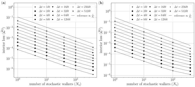
Figure 2: Empirical interior training loss for various walker size $N_{s}$ (horizontal axis) and time interval $\Delta t$ (different line types). (a) $m=1$ and (b) $m=3$.

To investigate the dependency of training trajectory on the choice of the time interval $\Delta t$ and the number of stochastic walkers $N_{s}$, we solve the problem with various combinations of these two parameters while keeping the other parameters fixed. Regarding the network structure, we use a standard multilayer perceptron (MLP) with three hidden layers, each comprising $200$ neurons and employing the ReLU activation function. The neural network is trained using the Adam optimizer [12] with learning parameters $\beta_{1}=0.99$ and $\beta_{2}=0.99$. At each iteration, we randomly sample $N_{r}=2000$ interior and $N_{b}=400$ boundary points from the uniform distribution. We consider ten different time intervals $\Delta t=2^{p}$, $p=0,1,2,\cdots,9$ and six different stochastic walker sizes $N_{s}=1,4,10,40,100,400$, resulting in a total of sixty combinations of $(\Delta t,N_{s})$. In considering the randomness of the training procedure, we run ten independent trials with extensive $1.5\times 10^{5}$ iterations for each parameter pair, which guarantees the convergence of the training loss.

4.2 Experiment results

We use the average interior training loss out of 10 trials to measure the training loss bias in Theorem 1, which we call ‘training loss.’ We also consider two problems with different wavenumber $m=1$ and $3$ for Eq. (63). We consider two solutions with $m=1$ and $m=2$ to check the contribution from the different magnitude $\ell_{2}$ norms of the gradient.

Figure 2 shows the log-log plot of the training loss after convergence as a function of the walker size $N_{s}$ (horizontal axis) with various $\Delta t$ (different line types). Figure 2 (a) and (b) are the cases with $m=1$ and $3$, respectively, and we can see that the training loss has a larger value for the more complicated case $m=3$ (about three times larger than the case of $m=1$), which the gradient magnitudes can explain for $m=1$ and $m=3$. As the analysis in the previous section predicts, the training loss decreases as the walker size increases for both cases, which aligns with the reference line of $\frac{1}{N_{s}}$ (dash-dot).

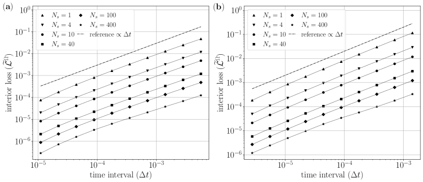
Figure 3: Empirical interior training loss for various time interval $\Delta t$ (horizontal axis) and walker size $N_{s}$ (different line types). (a) $m=1$ and (b) $m=3$.

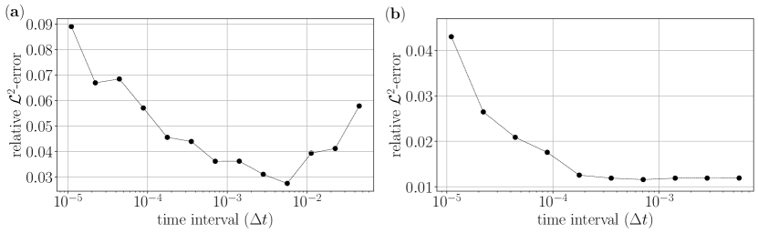
Figure 4: Relative $\mathcal{L}^{2}$ test error for varying time interval $\Delta t$. (a) $N_{s}=1$ (b) $N_{s}=400$.

In comparison between different line types, we can also check that the training loss decreases as the time interval $\Delta t$ decreases. The (linear) dependence of the training loss on $\Delta t$ is more explicit in Figure 3. Figure 3 shows the training loss as a function of $\Delta t$ (horizontal axis) with various $N_{s}$ (different line types). As in the previous figure, Figure 3 (a) and (b) show the results for the solution with $m=1$ and $3$, respectively. Compared to the reference line of $\Delta t$ (dash-dot), all training losses show a linear increase as $\Delta t$ increases.

We now check the test error after the training loss converges. In particular, we use the relative $\mathcal{L}^{2}$ error as a performance measure, calculated using the $1001\times 1001$ uniform grid. We want to note that a small training loss does not always imply a small test error. In DFLM, if $\Delta t$ is sufficiently small, the left- and right-hand sides of Eq. (4) get close enough that the training loss can be small for an arbitrary initial guess, which fails to learn the PDE solution.

For the case of $N_{s}=1$ and $400$, Figure 4 shows the relative $\mathcal{L}^{2}$ test error as $\Delta t$ increases for the solution Eq. (63) with $m=1$.

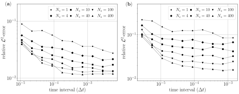
Figure 5: Relative $\mathcal{L}^{2}$ test error as a function of time interval $\Delta t$ for various $N_{s}$ values. (a) $m=1$ and (b) $m=3$.

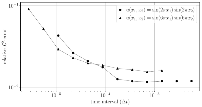
Figure 6: Relative $\mathcal{L}^{2}$ test error as a function of time interval $\Delta t$ for the two solutions with $m=1$ (simple) and $m=3$ (more oscillatory). $N_{s}$ is fixed at $400$.

When $\Delta t$ is small ($\leq 5\times 10^{-3}$), on the other hand, we can check that the training loss bias cannot explain the performance anymore. The test error increases as $\Delta t$ decreases regardless of the size of $N_{s}$. In other words, the result shows that the time interval $\Delta t$ must be sufficiently large for the network to learn the PDE solution by minimizing the training loss. When the training loss bias makes a non-negligible contribution with $N_{s}=1$, the test error can obtain the minimal value with an optimal $\Delta t\approx 5\times 10^{-3}$. If the bias contribution is small with $N_{s}=400$, the test error will be minimal with $\Delta t\geq 5\times 10^{-3}$. The increasing test error for decreasing $\Delta t$ is similar for other values of $N_{s}$ and solution types. Figure 5 shows the test relative error as a function of $\Delta t$ for the two solutions with $m=1$ (a) and $3$ (b) for various values of $N_{s}$. As $\Delta t$ decreases, the test error increases. Also, as $N_{s}$ decreases, which increases the sampling error in calculating the expectation, the test error increases for both solutions.

From Figure 6, which shows the test error of both solutions with $N_{s}=400$ and various $\Delta t$ values, we can also see that the optimal $\Delta t$ is related to the local variations of the solution. First, as we mentioned before, the solution with $m=3$ has a larger error as its gradient $\ell_{2}$ norm is larger than that of $m=1$, related to the loss bound and training update. Also, we use the same network structure, and all other parameters are equal for both solutions. Thus, it is natural to expect a much larger test error in the more complicated solution with $m=3$ than in the case of $m=1$. In comparison between the two solutions, we find that the test error of the more oscillatory solution ($m=3$) stabilizes much faster for a small $\Delta t$. That is, even using a small $\Delta t$, which yields a small neighborhood to explore and average, the more oscillatory solution case can see more variations than the simple solution case. Thus, the training loss can lead to a trainable result. Quantitatively, the optimal time intervals between the two solutions differ by a factor of about ten (that is, the more oscillatory solution can use $\Delta t$ ten times smaller than the one of the simple solution). This difference can be explained by the fact that the variance of the stochastic walkers is proportional to $\Delta t$, or the standard deviation is proportional to $\sqrt{\Delta t}$. As the more oscillatory solution has a wavenumber three times larger than the simple case, we can see that nine times shorter $\Delta t$ will cover the same variations as in the simple case, which matches the numerical result.

5 Discussions and conclusions

The derivative-free loss method (DFLM) uses the Feynman-Kac formulation to train a neural network to satisfy a PDE in the form of (1). In this study, we analyze the training loss bias and show that the training loss is asymptotically unbiased as $N_{s}$, the number of walkers at a collocation point, increases. The bias is also proportional to the time interval $\Delta t$, the time period for stochastic walkers to run for the expectation. We also showed that $\Delta t$ must be sufficiently large to guarantee a significant change in the training loss to make a meaningful update to find the PDE solution. Our numerical results also show that there exists a lower bound for the time interval $\Delta t$, which can depend on the local variations of the solution. Regarding computational efficiency, the analysis tells us that DFLM requires finding the optimal lower bound for the time interval and then choosing $N_{s}$ as small as possible based on the time interval.

Although we suspect that the lower bound for $\Delta t$ depends on the characteristics of the PDE solution, such as local variations, we do not have a quantitative method to specify the lower bound at the moment. It is natural to extend to current work to develop an approach to find the optimal lower bound of the time interval. We also plan to work on the optimal lower bound for multiscale solutions of different wave components. As the lower bound of the time interval shrinks as the solution has more highly oscillatory behaviors, it is natural to speculate how the lower bound behaves for such multiscale solutions. Along this line, we consider adaptive or hierarchical time stepping following the hierarchical learning approach [6]. The hierarchical time stepping can incorporate different time intervals for various scale components of the solution and use a hierarchical training procedure to expedite the learning process, which we leave as future work.

References

- [1] T. E. Booth, Exact monte carlo solution of elliptic partial differential equations, Journal of Computational Physics, 39 (1981), pp. 396–404.
- [2] S. Cai, Z. Mao, Z. Wang, M. Yin, and G. E. Karniadakis, Physics-informed neural networks (pinns) for fluid mechanics: a review, Acta Mechanica Sinica, 37 (2021), pp. 1727–1738.
- [3] G. Cybenko, Approximation by superpositions of a sigmoidal function, Mathematics of Control, Signals and Systems, 2 (1989), pp. 303–314.
- [4] W. E and B. Yu, The deep ritz method: A deep learning-based numerical algorithm for solving variational problems, Communications in Mathematics and Statistics, 6 (2018), pp. 1–12.
- [5] J. Han, A. Jentzen, and W. E, Solving high-dimensional partial differential equations using deep learning, Proceedings of the National Academy of Sciences, 115 (2018), pp. 8505–8510.
- [6] J. Han and Y. Lee, Hierarchical learning to solve pdes using physics-informed neural networks, in Computational Science – ICCS 2023, J. Mikyška, C. de Mulatier, M. Paszynski, V. V. Krzhizhanovskaya, J. J. Dongarra, and P. M. Sloot, eds., Cham, 2023, Springer Nature Switzerland, pp. 548–562.
- [7] J. Han and Y. Lee, A neural network approach for homogenization of multiscale problems, Multiscale Modeling & Simulation, 21 (2023), pp. 716–734.
- [8] J. Han, M. Nica, and A. R. Stinchcombe, A derivative-free method for solving elliptic partial differential equations with deep neural networks, Journal of Computational Physics, 419 (2020), p. 109672.
- [9] K. Hornik, M. Stinchcombe, and H. White, Multilayer feedforward networks are universal approximators, Neural Networks, 2 (1989), pp. 359–366.
- [10] C.-O. Hwang, M. Mascagni, and J. A. Given, A feynman–kac path-integral implementation for poisson’s equation using an h-conditioned green’s function, Mathematics and computers in simulation, 62 (2003), pp. 347–355.
- [11] I. Karatzas and S. Shreve, Brownian motion and stochastic calculus, vol. 113, Springer Science & Business Media, 1991.
- [12] D. P. Kingma and J. Ba, Adam: A method for stochastic optimization, 2014.
- [13] B. Oksendal, Stochastic differential equations: an introduction with applications, Springer Science & Business Media, 2013.
- [14] K. M. S. Park and A. R. Stinchcombe, Deep reinforcement learning of viscous incompressible flow, Journal of Computational Physics, 467 (2022), p. 111455.
- [15] S. Pauli, R. N. Gantner, P. Arbenz, and A. Adelmann, Multilevel monte carlo for the feynman–kac formula for the laplace equation, BIT Numerical Mathematics, 55 (2015), pp. 1125–1143.
- [16] M. Raissi, P. Perdikaris, and G. E. Karniadakis, Physics-informed neural networks: A deep learning framework for solving forward and inverse problems involving nonlinear partial differential equations, J. Comput. Phys., 378 (2019), pp. 686–707.
- [17] J. Sirignano and K. Spiliopoulos, Dgm: A deep learning algorithm for solving partial differential equations, Journal of Computational Physics, 375 (2018), pp. 1339–1364.
- [18] Y. Zhou and W. Cai, Numerical solution of the robin problem of laplace equations with a feynman–kac formula and reflecting brownian motions, Journal of Scientific Computing, 69 (2016), pp. 107–121.