Safe Non-Stochastic Control of Control-Affine Systems:
An Online Convex Optimization Approach

Abstract

We study how to safely control nonlinear control-affine systems that are corrupted with bounded non-stochastic noise, i.e., noise that is unknown a priori and that is not necessarily governed by a stochastic model. We focus on safety constraints that take the form of time-varying convex constraints such as collision-avoidance and control-effort constraints. We provide an algorithm with bounded dynamic regret, i.e., bounded suboptimality against an optimal clairvoyant controller that knows the realization of the noise a priori. We are motivated by the future of autonomy where robots will autonomously perform complex tasks despite real-world unpredictable disturbances such as wind gusts. To develop the algorithm, we capture our problem as a sequential game between a controller and an adversary, where the controller plays first, choosing the control input, whereas the adversary plays second, choosing the noise’s realization. The controller aims to minimize its cumulative tracking error despite being unable to know the noise’s realization a priori. We validate our algorithm in simulated scenarios of (i) an inverted pendulum aiming to stay upright, and (ii) a quadrotor aiming to fly to a goal location through an unknown cluttered environment.

I Introduction

In the future, robots will be leveraging their on-board control capabilities to complete safety-critical tasks such as package delivery [1], target tracking [2], and disaster response [3]. To complete such complex tasks, the robots need to efficiently and reliably overcome a series of key challenges:

Challenge I: Time-Varying Safety Constraints

The robots need to ensure the safety of their own and of their surroundings. For example, robots often need to ensure that they follow collision-free trajectories, or that their control effort is kept under prescribed levels. Such safety requirements take the form of time-varying state and control input constraints: e.g., as robots move in cluttered environments, the current obstacle-free environment changes (Figure 1). Accounting for such constraints in real-time can be challenging, requiring increased computational effort [4, 5]. Hence, several real-time state-of-the-art methods do not guarantee safety at all times [6, 7].

Challenge II: Unpredictable Noise

The robots’ dynamics are often corrupted by unknown non-stochastic noise, i.e., noise that is not necessarily i.i.d. Gaussian or, more broadly, that is not governed by a stochastic (probability) model. For example, aerial and marine vehicles often face non-stochastic winds and waves, respectively [8]. But the current control algorithms primarily rely on the assumption of known stochastic noise, typically, Gaussian, compromising the robots’ ability to ensure safety in real-world settings where this assumption is violated [9].

Challenge III: Nonlinear, Control-Affine Dynamics

The dynamics of real-world robots are often nonlinear, in particular, control-affine. For example, the dynamics of quadrotors and marine vessels take the form of $x_{t+1}=f\left(x_{t}\right)+g\left(x_{t}\right)u_{t}+w_{t}$, where (i) $x_{t}$ is the robot’s state, (ii) $f\left(x_{t}\right)$ and $g\left(x_{t}\right)$ are system matrices characterizing the robot’s dynamics, (iii) $u_{t}$ is the control input, and (iv) $w_{t}$ is the disturbance [10]. Handling nonlinear dynamics often requires complex control policies, requiring, in the most simple case, linearization at each time step, and, thus, additional computational effort [4].

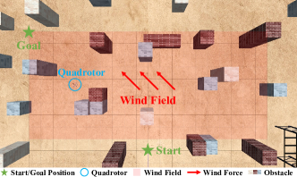
Figure 1: Safe non-stochastic control example: Autonomous flight in cluttered environments subject to unknown wind disturbances. In this paper, we focus on safe non-stochastic control of control-affine systems where the robots’ capacity to select effective control actions fast is challenged by (i) time-varying safety constraints, (ii) unknown, unstructured, and, more broadly, unpredictable noise, and (iii) nonlinear control-affine dynamics. For example, in package delivery with quadrotors, the quadrotors are required to fly to goal positions. But during such tasks, (i) the quadrotors need to ensure collision avoidance at all times, which requires control actions that respect time-varying state and control-input constraints, (ii) the quadrotors may be disturbed by unpredictable wind gusts, and (iii) they need to account for their nonlinear, in particular, control-affine dynamics. These challenges stress the quadrotors’ ability to decide effective control inputs fast, and to ensure safety. We aim to provide a control algorithm that handles these challenges, guaranteeing bounded suboptimality against optimal safe controllers in hindsight.

The above challenges motivate control methods that efficiently and reliably handle control-affine systems, and guarantee the satisfaction of time-varying safety constraints even in the presence of non-stochastic noise. State-of-the-art methods to this end typically rely on robust control [11, 12, 13, 14, 15, 16] or on online learning [17, 18, 19, 20, 21, 22, 23]. But the robust methods are often conservative and computationally heavy: not only they simulate the system dynamics over a lookahead horizon; they also assume a worst-case noise realization, given a known upper bound on the magnitude of the noise. To reduce conservatism and increase efficiency, researchers have also focused on online learning methods via Online Convex Optimization (OCO) [24]. These methods rely on the Online Gradient Descent (OGD) algorithm or its variants, offering bounded regret guarantees, i.e., bounded suboptimality with respect to an optimal (possibly time-varying) clairvoyant controller that knows the future noise realization a priori [17, 18, 19, 20, 22]. However, the current online methods address only linear dynamical systems and time-invariant safety constraints.

Contributions. We provide an algorithm for the problem of controlling control-affine systems, guaranteeing their safety against time-varying safety constraints even in the presence of non-stochastic noise. Henceforth, we refer to this problem as Safe Non-Stochastic Control for Control-Affine Systems (Safe-NSC). Our solution approach, its generality, and its performance guarantees are as follows:

Approach

We first formalize the problem of Safe-NSC as a sequential game between a controller and an adversary, inspired by the current literature on online learning and control [17, 18, 19, 20, 22, 23]: at each time step $t$, the controller plays first, choosing a control input, and, then, the adversary plays second, choosing the noise’s realization. The controller aims to minimize its cumulative performance, e.g., tracking error, despite being unaware of the noise’s realization a priori.

We then provide an algorithm for Safe-NSC, called Safe Online Gradient Descent (Safe-OGD) (Algorithm 1). Safe-OGD chooses control input $u_{t}$ online from a set ${\cal U}_{t}$ that is also chosen by Safe-OGD online to guarantee safety. In more detail, ${\cal U}_{t}$ is constructed (i) given the current safety constraints, and an upper bound to the non-stochastic noise, and (ii) employing Control Barrier Functions (CBF) [25] to enforce the constraints. The safety constraints may be known a priori or constructed online given the currently known environment, e.g., the current obstacle-free environment within field of view.

Generality

Safe-OGD, as presented above, selects control inputs directly, without optimizing an underlying policy parameterization. Oftentimes, however, it is desired to optimize a control-policy parametrization, such as in Linear-Quadratic Gaussian (LQG) control [26]. We show that Safe-OGD can be extended to optimize online any control-policy parameterization that is linear in the parameters (Section IV-C). Examples of such policies include the linear state-feedback control policy [26], which is commonly used for LQG control, and the disturbance-action policy [5, 17], which is commonly used for non-stochastic control.

Performance Guarantees and Near-Optimality in Classical Control Settings

We prove that the Safe-OGD controller has bounded dynamic regret against any clairvoyant control policy (Theorem 1). The regret bound also implies (near-)optimal performance in classical online convex optimization and optimal control problems: (i) when the domain of optimization is time-invariant, Safe-OGD’s performance bound reduces to that of the seminal OGD algorithm for online convex optimization, which bound is near-optimal [27]; and (ii) when also the optimal clairvoyant control policy is time–invariant, Safe-OGD learns asymptotically the optimal control policy (Section V), implying, for example, that Safe-OGD would converge to the optimal linear state-feedback controller if applied to the classical LQG problem.

Numerical Evaluations. We validate our algorithms with extensive simulations (Section VI). Specifically, we validate our algorithm in simulated scenarios of (i) an inverted pendulum that is tasked to stay upright, and (ii) a quadrotor that is tasked to move to a prescribed location by flying through an unknown cluttered environment (Fig. 1). We conduct these experiments in Python and Gazebo, respectively. In the inverted pendulum experiment (Section VI-A), we compare our algorithm with a linear feedback controller, the Deep Deterministic Policy Gradient (DDPG) controller [28, 29], and the iterative Linear–Quadratic Regulator (iLQR) [6]. In the quadrotor experiment (Section VI-B), we compare our algorithm with the geometric controller [30] and a Robust Nonlinear Model Predictive Controller (R-NMPC) [31].

Our algorithm achieves in the simulations a better performance, achieving (i) safety at all times, whereas the iLQR and geometric controllers as well as R-NMPC do not, and (ii) better or comparable tracking performance than the linear feedback, DDPG, and geometric controllers as well as R-NMPC.

II Related Work

The said Challenges I to III have motivated research on robust control, online learning for control, and safe control:

Robust control. Robust control algorithms select control inputs upon simulating the future system dynamics across a lookahead horizon [32, 12, 13, 14, 15, 16]. To this end, they either assume a worst-case realization of noise, given an upper bound to the magnitude of the noise [12, 13, 14, 15, 16], or assume a stochastic model governing the evolution of the noise [32]. However, assuming the worst-case noise realization can oftentimes be pessimistic; and assuming a stochastic model may compromise performance when the underlying noise is non-stochastic or the assumed model is incorrect.

Online learning for control. Online learning algorithms select control inputs based on past information only since they assume no model that can be used to simulate the future evolution of the noise [17, 19, 18, 20, 21, 22, 23]. Assuming a known upper bound to the magnitude of the noise, and by employing the OCO framework to capture the non-stochastic control problem as a sequential game between a controller and an adversary [24], they provide bounded regret guarantees against an optimal (time-varying) clairvoyant controller even under unpredictable noise. They consider time-invariant state and control input constraints or no constraint, in contrast to time-varying safety constraints, with the exception of [23]. Also, they only consider linear dynamical systems, in contrast to nonlinear control-affine systems, with the exception of [21].

Safe Control. Safe control algorithms select control inputs to ensure that the unsafe region on the system’s state space is not reachable. This can be achieved by using Hamilton-Jacobi (HJ) reachability analysis [33] and CBF [25]. HJ reachability analysis computes the backward reachable set, i.e., the set of states from which the system can be driven into the unsafe set, and selects control inputs to avoid such an unsafe set. HJ reachability analysis is able to handle bounded disturbances and recovers maximal safe sets. However, it is often computationally intractable for high-dimensional systems, thus, requiring to place assumptions on system dynamics to recover traceability, such as requiring linear systems or the system dynamics can be decomposed into several subsystems [34, 35, 36]. CBF achieves safety by ensuring forward invariance of the safe set, i.e., by selecting control inputs such that the system state remains in the safe set. This method has been used to design control algorithms for systems with no noise [25, 37, 38, 39], stochastic noise [40, 7], and bounded non-stochastic noise [41].

III Problem Formulation

We formulate the problem of Safe Non-Stochastic Control for Control-Affine Systems (1). To this end, we use the following framework and assumptions.

Control-Affine Systems. We consider discrete-time control-affine systems of the form

$$x_{t+1}=f\left(x_{t}\right)+g\left(x_{t}\right)u_{t}+w_{t},\quad t\in\{1,\ldots,T\},\vspace{-1.5mm}$$ (1)

where $x_{t}\in\mathbb{R}^{d_{x}}$ is the state, $u_{t}\in\mathbb{R}^{d_{u}}$ is the control input, $w_{t}\in\mathbb{R}^{d_{x}}$ is the process noise, and $f:\mathbb{R}^{d_{x}}{\color[rgb]{0,0,1}\rightarrow}\mathbb{R}^{d_{x}}$ and $g:\mathbb{R}^{d_{x}}{\color[rgb]{0,0,1}\rightarrow}\mathbb{R}^{d_{x}}\times\mathbb{R}^{d_{u}}$ are known locally Lipschitz functions.

For simplicity, we assume the stability of the nominal system in eq. 1 without the noise:

Assumption 1 (Stability of the Nominal System).

The nominal system, $x_{t+1}=f\left(x_{t}\right)+g\left(x_{t}\right)u_{t}$, is stable.

Remark 1 (Removal of the Stability Condition).

The stability condition can be removed by employing a known stabilizing controller $u_{t}^{s}$, that is, setting $u_{t}=u_{t}^{s}+v_{t}$, where the stabilizing controller $u_{t}^{s}$ can be computed via Control Lyapunov Functions [42], and $v_{t}$ is the controller to be designed.

For a quadrotor, such a stabilizing controller can be one that enables the quadrotor to track a given reference path [43].

Assumption 2 (Bounded Noise).

The noise is bounded, i.e., $w_{t}\in{\cal W}\triangleq\{w\mid\left\|w\right\|\leq W\}$, where $W$ is given.

Per 2, we assume no stochastic model for the process noise $w_{t}$: the noise may even be adversarial, subject to the bound $W$. An example is a quadrotor subject to wind disturbances with bounded magnitude, whose evolution may not be governed by a known stochastic model.

Safety Constraints. We consider the states and control inputs for all $t$ must satisfy polytopic constraints of the form

$$x_{t}\in{\cal S}_{t}\triangleq\{x\mid L_{x,t}x\leq l_{x,t}\},\ \forall\{{w}_{\tau}\in{\cal W}\}_{\tau=1}^{t-1},$$ (2)

$$u_{t}\in{\cal C}_{t}\triangleq\{u\mid L_{u,t}u\leq l_{u,t}\},$$

where $L_{x,t}$, $l_{x,t}$, $L_{u,t}$, and $l_{u,t}$ are given.

Assumption 3 (Bounded State and Control Input Domain).

The domain sets ${\cal S}_{t}$ and ${\cal C}_{t}$ are bounded for all $t\in\{1,\dots,T\}$. Also, they are contained in the bounded sets $\mathcal{S}$ and ${\cal C}$, respectively, that both contain the zero point and have diameter $D$.

3 ensures that the loss function has a bounded gradient with respect to the state and control input; this helps to quantify Safe-OGD’s dynamic regret. Bounded state constraints emerge, for example, when a quadrotor flies in a cluttered environment (Fig. 1): its state must be in a bounded flight corridor to ensure safety. Bounded control input constraints are needed to avoid controller saturation.

Assumption 4 (Existance of Safe Controller).

Given $x_{t}\in{\cal S}_{t}$, there exists a safe controller $u_{t}\in{\cal C}_{t}$ such that $x_{t+1}\in{\cal S}_{t+1}$, $\forall w_{t}\in{\cal W}$.

4 enables the constraint $L_{x,t}x\leq l_{x,t}$ to be used as a CBF, introduced in Section IV-A. This assumption is reasonable if the robot is kept at a low speed and the control authority is large enough such that the robot is able to react quickly and keep safe even if it is close to an obstacle. In general, the constraint $L_{x,t}x\leq l_{x,t}$ must be constructed by taking into account the robot’s speed and acceleration capacity such that there always exists a control input $u_{t}$ that satisfies $x_{t+1}\in{\cal S}_{t+1}$, an example of which is given in [25].

Control Performance Metric. We design the control inputs $u_{t}$ to ensure: (i) safety; and (ii) a control performance that is comparable to an optimal clairvoyant policy that knows the future noise realizations ${w}_{1},w_{2},\ldots$ a priori. Particularly, we consider the control performance metric defined below.

Definition 1 (Dynamic Regret).

Assume a lookahead time horizon of operation $T$, and loss functions $c_{t}$, $t=1,\ldots,T$. Then, dynamic regret is defined as

$$\operatorname{Regret-NSC}_{T}^{D}=\sum_{t=1}^{T}c_{t}\left(x_{t+1},u_{t}\right)-\sum_{t=1}^{T}c_{t}\left(x_{t+1}^{*},u_{t}^{*}\right),\vspace{-2mm}$$ (3)

where (i) both sums in eq. 3 are evaluated with the same noise $\{w_{1},\ldots,w_{T}\}$ that is the noise experienced by the system during its evolution per the control sequence $\{u_{1},\ldots,u_{T}\}$, (ii) $u_{t}^{*}$ is the optimal control input in hindsight, i.e., the optimal input given a priori knowledge of the noise $w_{t}$, which includes the control inputs generated by a nonlinear control policy, (iii) $x_{t+1}^{*}$ is the state reached by applying the optimal control inputs $u_{t}^{*}$ from state $x_{t}$, which is the optimal state could have been reached when the system is at $x_{t}$, and (iv) $x_{t+1}^{*}$ and $u_{t}^{*}$ satisfy the constraints in eq. 2 for all $t$.

Assumption 5 (Convex and Bounded Loss Function, and with Bounded Gradient).

$c_{t}\left(x_{t+1},u_{t}\right):\mathbb{R}^{d_{x}}\times\mathbb{R}^{d_{u}}{\color[rgb]{0,0,1}\rightarrow}\mathbb{R}$ is convex in $x_{t+1}$ and $u_{t}$. Further, when $\|x\|$ and $\|u\|$ are bounded, then $\left|c_{t}(x,u)\right|$, $\left\|\nabla_{x}c_{t}(x,u)\right\|$, and $\left\|\nabla_{u}c_{t}(x,u)\right\|$ are also bounded.

A loss function that satisfies 5 is the commonly used quadratic cost $c_{t}\left(x_{t+1},u_{t}\right)=x_{t+1}Qx_{t+1}^{\top}+u_{t}Ru_{t}^{\top}$.

Problem Definition. We formally define the problem of Safe Non-Stochastic Control of Control-Affine Systems:

Problem 1 (Safe Non-Stochastic Control of Control-Affine Systems (Safe-NSC)).

Assume that the initial state of the system is safe, that is, $x_{1}\in{\cal S}_{1}$. At each $t=1,\ldots,T$, identify a control input $u_{t}$ that guarantees safety, that is, $x_{t}\in{\cal S}_{t}$ and $u_{t}\in{\cal C}_{t}$, and such that $\operatorname{Regret-NSC}_{T}^{D}$ is minimized by time $T$.

IV Algorithm for Safe Non-Stochatic Control

We present the Safe Online Gradient Descent (Safe-OGD) algorithm (Algorithm 1). We first provide background information on control barrier functions since Safe-OGD utilizes them to ensure safety (Section IV-A). Then, we present the basic version of Safe-OGD that directly optimizes the control inputs (Section IV-B). Finally, we discuss how the algorithm is extended to optimize linear control policies (Section IV-C).

IV-A Preliminaries: Discrete-Time Control Barrier Functions

Consider a smooth function $h:\mathbb{R}^{d_{x}}{\color[rgb]{0,0,1}\rightarrow}\mathbb{R}$, a safety set $\mathcal{D}$ and its boundary defined as $\mathcal{D}\triangleq\{x\in\mathbb{R}^{d_{x}}\mid h\left(x\right)>0\}$, $\partial\mathcal{D}\triangleq\{x\in\mathbb{R}^{d_{x}}\mid h\left(x\right)=0\}$.

Definition 2 (Discrete-Time Exponentially Control Barrier Function) (DCBF) [38]).

A map $h:\mathbb{R}^{d_{x}}{\color[rgb]{0,0,1}\rightarrow}\mathbb{R}$ is a Discrete-Time Exponentially Control Barrier Function on ${\cal D}$ if there exists a control input $u_{t}\in{\cal C}_{t}$ and a positive constant $\alpha~{}\in~{}(0,1]$ such that $\Delta h_{t}\triangleq h\left(x_{t+1}\right)-h\left(x_{t}\right)$ satisfies

$$\Delta h_{t}+\alpha h\left(x_{t}\right)\geq 0.\vspace{-1.5mm}$$ (4)

The value of DCBFs in control is that they can be used to ensure safety: a control input $u_{t}$ renders the safety set $\mathcal{D}$ forward invariant when eq. 4 is satisfied.

IV-B Safe-OGD Algorithm: The Basic Algorithm

0:  Time horizon $T$; gradient descent step size $\eta$. 0:  Control ${u}_{t}$ at each time step $t=1,\ldots,T$. 1:  Initialize ${u}_{1}\in{\cal U}_{1}$; 2:  for each time step $t=1,\dots,T$ do 3:     Apply control input $u_{t}$; 4:     Observe the state $x_{t+1}$, and calculate the noise $w_{t}=x_{t+1}-f(x_{t})-g(x_{t})u_{t}$; 5:     Suffer the loss $c_{t}(x_{t+1},u_{t})$; 6:     Express the loss function in $u_{t}$ as $c_{t}(u_{t})\triangleq c_{t}(x_{t+1},u_{t})=c_{t}(f(x_{t})+g(x_{t})u_{t}+w_{t},u_{t})$; 7:     Calculate gradient $\nabla_{t}\triangleq\nabla_{u}c_{t}(x_{t+1},u_{t})$; 8:     Calculate domain set ${\cal U}_{t+1}$ per eq. 5; 9:     Update $u_{t+1}^{\prime}=u_{t}-\eta\nabla_{t}$; 10:     Project $u_{t+1}^{\prime}$ onto ${\cal U}_{t+1}$, i.e., $u_{t+1}=\Pi_{{\cal U}_{t+1}}(u_{t+1}^{\prime})$; 11:  end for

Algorithm 1 Safe Non-Stochastic Control Algorithm for Control-Affine Systems.

We present Safe-OGD in Algorithm 1. The algorithm first initializes $u_{1}\in{\cal U}_{1}$ (line 1). At each iteration $t$, Algorithm 1 evolves to state $x_{t+1}$ applying the control inputs $u_{t}$ (line 3) and calculates the noise $w_{t}$ upon observation of $x_{t}$ (line 4). After that, the algorithm suffers a loss of $c_{t}\left(x_{t+1},u_{t}\right)$ (line 5). Then, Algorithm 1 expresses $c_{t}\left(x_{t+1},u_{t}\right)$ as a function of $u_{t}$, i.e., $c_{t}(u_{t})\triangleq c_{t}(x_{t+1},u_{t})=c_{t}(f(x_{t})+g(x_{t})u_{t}+w_{t},u_{t})$ —which is convex in $u_{t}$, given functions $f\left(\cdot\right)$ and $g\left(\cdot\right)$, $x_{t}$, and $w_{t}$, per Lemma 1 below— and obtains the gradient $\nabla_{t}\triangleq\nabla_{u}c_{t}\left(x_{t+1},u_{t}\right)$ (lines 6-7). To ensure safety, Algorithm 1 constructs the domain set ${\cal U}_{t+1}$ per Lemma 2 (line 8). Finally, Algorithm 1 updates the control gain and projects it back to the domain set ${\cal U}_{t+1}$ (lines 9-10).

Lemma 1 (Convexity of Loss function in Control Input).

The loss function $c_{t}\left(x_{t+1},u_{t}\right):\mathbb{R}^{d_{x}}\times\mathbb{R}^{d_{u}}{\color[rgb]{0,0,1}\rightarrow}\mathbb{R}$ is convex in the control input $u_{t}$, given functions $f\left(\cdot\right)$ and $g\left(\cdot\right)$, $x_{t}$, and $w_{t}$.

Lemma 2 (Construction of Time-Varying Domain Set with Safety Guarantee).

Algorithm 1 guarantees $x_{t+1}\in{\cal S}_{t+1}$ and $u_{t}\in{\cal C}_{t}$ at each time step $t$ by choosing $u_{t}\in{\cal U}_{t}$, where

$${\cal U}_{t}\triangleq\{u\mid \ L_{u,t}u\leq l_{u,t},$$ (5)

$$-L_{x,t+1}g\left(x_{t}\right)u-\left\|L_{x,t+1}\right\|W+l_{x,t+1}$$

$$-L_{x,t+1}f\left(x_{t}\right)-(1-\alpha)\left(l_{x,t}-L_{x,t}x_{t}\right)\geq 0\}.$$

The origin of the two inequalities in eq. 5 are as follows: the first condition is due to the requirement $u_{t}\in{\cal C}_{t}$; and the second condition is the result of applying the DCBF condition in eq. 4 to guarantee $x_{t+1}\in{\cal S}_{t+1}$.

IV-C Extension of Safe-OGD to Linear Control Policies

We extend Algorithm 1 to optimize any linearly parameterized control policy in the form of control parameters multiplying state or noise, e.g., the linear state-feedback policy [26] and the disturbance-action policy [5, 17]:

• Linear State-Feedback Control Policy: This policy takes the form of $u_{t}=-K_{t}x_{t}$, where $K_{t}\in\mathbb{R}^{d_{u}\times d_{x}}$ is the control parameterization, and $\|K_{t}\|\leq\kappa$ with $\kappa>0$.

• Disturbance-Action Control Policy: This policy is defined as $u_{t}=\sum_{i=1}^{H}K_{t}^{[i]}w_{t-i}$, where $K_{t}=(K_{t}^{[1]},\dots,K_{t}^{[H]})\in\mathbb{R}^{H\times d_{u}\times d_{x}}$ is the control parameterization, $H$ is a positive integer, and $\|K_{t}^{[i]}\|\leq\kappa$.

The extension of Lemma 1 follows trivially as $u_{t}$ is linear in $K_{t}$. The extension of Lemma 2 follows by substituting $u_{t}$ with the choice of control policy, e.g., $-Kx_{t}$, and $\sum_{i=1}^{H}K^{[i]}w_{t-i}$.

Modification of Algorithm 1 to Learning Linearly Parameterized Control Policies. To enable Algorithm 1 to learn linear control policies, the following modifications are needed:

• The domain sets ${\cal U}_{t}$ (lines 1, 8, 10) should be changed to ${\cal K}_{t}$, where ${\cal K}_{t}$ is the set of control parameterization that ensures safety, calculated based on Lemma 2 for $K_{t}$;

• The loss function $c_{t}$ (line 6) and the gradient (line 7) should be respected to the control parameterization $K_{t}$;

• The update and project steps (lines 9-10) are performed on the control parameterization $K_{t}$.

V Dynamic Regret Analysis

We present the dynamic regret bounds of Safe-OGD, both for the basic algorithm and for its extension to learning linearly parameterized control policies. We use the notation:

• $\bar{u}_{t+1}\triangleq\Pi_{{\cal U}_{t}}(u_{t+1}^{\prime})$ is the control would have been chosen at time step $t+1$ if ${\cal U}_{t}={\cal U}_{t+1}$;

• $\zeta_{t}\triangleq\left\|\bar{u}_{t+1}-{u}_{t+1}\right\|$ is the distance between $\bar{u}_{t+1}$ and ${u}_{t+1}$, which are the projection of ${u}_{t+1}^{\prime}$ onto sets ${\cal U}_{t}$ and ${\cal U}_{t+1}$, respectively. Thus, it quantifies how fast the safe domain set changes —$\zeta_{t}$ is $0$ when ${\cal U}_{t}={\cal U}_{t+1}$;

• $S_{T}\triangleq\sum_{t=1}^{T}\zeta_{t}$ is the cumulative variation of control due to time-varying domain sets. $S_{T}$ becomes $0$ when domain sets are time-invariant;

• $C_{T}\triangleq\sum_{t=2}^{T}\|u_{t-1}^{\star}-u_{t}^{\star}\|$ is the cumulative variation of the optimal control sequence. It quantifies how fast the optimal control input must change.

Theorem 1 (Dynamic Policy Regret Bound of Algorithm 1).

Assume $\eta={\cal O}\left(\frac{1}{\sqrt{T}}\right)$ for the gradient descend step size. Then, (i) when Algorithm 1 is employed to chose online control inputs $u_{1},u_{2},\ldots$, then it achieves

$$\operatorname{Regret-NSC}_{T}^{D}\leq{\cal O}\left(\sqrt{T}\left(1+C_{T}+S_{T}\right)\right),\vspace{-2mm}$$ (6)

against any control inputs $({u}^{\star}_{1},\dots,{u}^{\star}_{T})\in{\cal U}_{1}\times\cdots\times{\cal U}_{T}$.

(ii) When Algorithm 1 is employed to choose online control parameters $K_{1},K_{2},\ldots$, then it achieves

$$\operatorname{Regret-NSC}_{T}^{D}\leq{\cal O}\left(\sqrt{T}\left(1+C_{T}+S_{T}\right)\right),\vspace{-2mm}$$ (7)

against any control policies $({K}^{\star}_{1},\dots,{K}^{\star}_{T})\in{\cal K}_{1}\times\cdots\times{\cal K}_{T}$, where $C_{T}\triangleq\sum_{t=2}^{T}\|K_{t-1}^{\star}-K_{t}^{\star}\|_{\mathrm{F}}$ and $S_{T}\triangleq\sum_{t=1}^{T}\left\|\Pi_{{\cal K}_{t}}(K_{t+1}^{\prime})-{K}_{t+1}\right\|_{\mathrm{F}}$.

The regret bounds in Theorem 1 reflect the difficulty of the safe non-stochastic control problem. Ideally, the bounds would be ${\cal O}(\sqrt{T})$, which would imply that Algorithm 1 asymptotically guarantees the same performance as the optimal clairvoyant controller because then $\lim_{T\rightarrow\infty}\operatorname{Regret-NSC}_{T}^{D}/T=0$. But the bounds depend on $C_{T}$ and $S_{T}$, which in the worst-case can make the regret linear in $T$:

Dependency on $S_{T}$

The bounds in Theorem 1 depend on $S_{T}$ due to the optimization domain sets being time-varying (Lemma 2): expectedly, when the safety sets change across time, while the system is threatened by non-stochastic noise, the control becomes more challenging, and, thus, it is more difficult for Algorithm 1 to match the performance of the optimal controller in hindsight. In contrast, $S_{T}$ is zero when the domain sets are time-invariant. Then, in particular, the regret bounds in Theorem 1 reduce to the near-optimal bounds for the standard OCO setting with time-invariant domain sets:

Remark 2 (Optimality under Time-Invariant Domain of Optimization).

When the optimization domain sets are time-invariant, that is, ${\cal U}_{1}\!=\!\ldots\!=\!{\cal U}_{T}$ (or ${\cal K}_{1}\!=\!\ldots\!=\!{\cal K}_{T}$), then $S_{T}=0$. Therefore, the regret bounds in Theorem 1 reduce to ${\cal O}\left(\sqrt{T}\left(1+C_{T}\right)\right)$, which are near-optimal [44], matching the regret bound of the seminal OGD algorithm for the standard OCO setting with time-invariant constraints [27].

More broadly, $S_{T}$ can be sublinear in applications where any two consecutive safe sets differ a little.

Dependency on $C_{T}$

The bounds in Theorem 1 depend on $C_{T}$ due to the optimal control sequence/policy being in general time-varying. Specifically, [44] proved that any optimal dynamic regret bound for OCO must depend on $C_{T}$, being lower bounded by $\Omega\left(\sqrt{T(1+C_{T})}\right)$. Expectedly, when the unknown noise sequence requires the system to adapt its control input frequently, then the harder for Algorithm 1 is to match the optimal control sequence.

Remark 3 (Optimality under also Time-Invariant Control Policies).

When both the domain sets and the optimal control input sequence in hindsight are time-invariant, i.e., $S_{T}=C_{T}=0$, then the regret bounds in Theorem 1 reduce to ${\cal O}\big{(}\sqrt{T}\big{)}$. This implies Safe-OGD converges to the optimal controller in hindsight since then $\lim_{T\rightarrow\infty}\operatorname{Regret-NSC}_{T}^{D}/T=0$. For example, the classical LQG optimal-control problem has an optimal solution with the form $u_{t}=-Kx_{t}$, where $K$ is time-invariant [26]. Thus, if we apply Safe-OGD to learn $K$, then Safe-OGD will converge to an optimal one.

VI Numerical Evaluations

TABLE I: Performance Comparison given the Pendulum System in Section VI-A. The table reports the average value and standard deviation of computational time and cumulative loss. The performance is quantified per the computational time, cumulative loss, and safety rate. The red numbers correspond to the worse performance.

	Computational Time ($ms$)	Cumulative Loss	Safety Rate
Ours	$21.6903\pm 7.8186$	$20.0022\pm 1.9933$	$100\%$
DDPG	$27.6517\pm 30.7014$	$26.4953\pm 1.1261$	$100\%$
iLQR	$575.6701\pm 14.7182$	$9.3902\pm 0.5825$	$60\%$
LF	$10.9756\pm 2.2418$	$26.6495\pm 1.2891$	$100\%$

We evaluate Algorithm 1 in extensive simulated scenarios of safe control, where the controller aims to track a reference setpoint/path while satisfying the state and control input constraints. Particularly, we first consider an inverted pendulum aiming to stay upright despite noise disturbances (Section VI-A) and learn a linear feedback policy. Then, we consider a quadrotor flying in cluttered environments subject to unknown external forces (Section VI-B) and learn directly the control input. Our algorithm is observed in the simulations to (i) achieve comparable or better tracking performance than the linear feedback, DDPG, geometric control, and R-NMPC, and (ii) guarantee the safety of the system, in contrast to the iLQR and geometric controllers, which violate the safety guarantees.

VI-A Inverted Pendulum

Simulation Setup. We consider an inverted pendulum model with the state vector its angle $\theta$ and angular velocity $\dot{\theta}$, and control input $u$ the torque. The goal of the pendulum is to stay at $(\theta,\dot{\theta})=(0,0)$. The dynamics of the pendulum are:

$$\theta_{t+1}=\theta_{t}+\Delta t\dot{\theta}_{t},\;\dot{\theta}_{t+1}=\frac{3g}{2l}\sin\theta_{t}+\frac{3\Delta t}{ml^{2}}u_{t},$$ (8)

where $g=10~{}m/s^{2}$ is the acceleration of gravity, $m=1kg$ is the mass, $l=1m$ is the length of the pendulum, and $\Delta t=0.05s$ is the time step. We use: $[-\pi/2\ -\pi/2]^{\top}~{}\leq[\theta_{t}\ \dot{\theta}_{t}]^{\top}~{}\leq~{}[\pi/2\ \pi/2]^{\top}$ and $-4~{}\leq~{}u_{t}~{}\leq~{}4$. We use the loss functions with the form of $c_{t}(\theta_{t+1},\dot{\theta}_{t+1},u_{t})=\theta_{t+1}^{2}+0.1\dot{\theta}_{t+1}^{2}+0.001u_{t}^{2}$ to learn a linear feedback controller.

We simulate the setting for $T~{}=~{}500$ time steps. We corrupt the system dynamics with process noise drawn for the Gaussian, Uniform, or Laplace distribution; and we assume $\|w_{t}\|\leq 0.1$. We perform the simulation $5$ times for each noise distribution in Python with CVXPY solver [45].

Compared Algorithms. We compare Algorithm 1 with: a linear feedback (LF) controller that stabilizes the linearized pendulum dynamics, the Deep Deterministic Policy Gradient (DDPG) [28, 29, 46], and the iterative linear–quadratic regulator (iLQR) [6]. The LF and DDPG handle the safety constraints by projecting the control input onto the safe domain set constructed by Lemma 2; the iLQR, instead, adds a penalty about the constraint violation to the objective function [6].

Results. The results are given in Table I. Algorithm 1 demonstrates better cumulative loss compared to DDPG and LF, achieving 100% safety rate. The iLQR, instead, achieves the lowest loss but only with a $60\%$ safety rate.

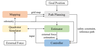
Figure 2: Autonomous system architecture in Section VI-B.

VI-B Quadrotor

TABLE II: Performance Comparison for the Quadrotor Experiments in Section VI-B. The table reports the average value and standard deviation of flight time, trajectory length, tracking error, and computational time. The red numbers correspond to the worse performance. Our method achieves better performance in terms of flight time, trajectory length, tracking error, and safety rate. [30] has the worst tracking error, resulting in low safety rates. [31] either collides due to latency or has longer flight time and length as it aims to guarantee safety against worst-case disturbances over a lookahead horizon.

Goal Position ($m$)	Disturbance ($m/s^{2}$)	Method	Flight Time ($s$)	Trajectory Length ($m$)	Tracking Error ($m$)	Safety Rate	Computational Time ($ms$)
							Planner	Controller
$\left[\begin{array}[]{ccc}14&-10&1\end{array}\right]^{\top}$	$\left[\begin{array}[]{ccc}2&2&0\end{array}\right]^{\top}$	Ours	$9.9720\pm 0.0944$	$18.0600\pm 0.6542$	$0.0811\pm 0.0130$	$100\%$	$0.8333\pm 2.8868$	$0.1837\pm 1.3433$
		[30]	$10.1433\pm 0.1914$	$18.0333\pm 0.2309$	$0.3022\pm 0.0078$	$60\%$	$0.7692\pm 2.7735$	$0.1049\pm 1.0192$
		[31]	$11.9675\pm 1.0678$	$19.0597\pm 0.7588$	$0.1657\pm 0.0055$	$80\%$	$10.0833\pm 1.8277$	$0.1091\pm 1.0392$
$\left[\begin{array}[]{ccc}10&10&1\end{array}\right]^{\top}$	$\left[\begin{array}[]{ccc}3&3&0\end{array}\right]^{\top}$	Ours	$8.7340\pm 0.2050$	$15.8600\pm 0.6877$	$0.1000\pm 0.0134$	$100\%$	$0.9091\pm 3.0151$	$0.1692\pm 1.2902$
		[30]	$10.2625\pm 0.2869$	$16.5250\pm 0.6185$	$0.2694\pm 0.0056$	$40\%$	$0.9091\pm 3.0151$	$0.1350\pm 1.1546$
		[31]	$10.4967\pm 0.6469$	$16.4467\pm 0.4520$	$0.1874\pm 0.0391$	$60\%$	$9.4624\pm 2.2616$	$0.1081\pm 1.0344$
$\left[\begin{array}[]{ccc}10&10&1\end{array}\right]^{\top}$	$\left[\begin{array}[]{ccc}-2&2&0\end{array}\right]^{\top}$ if $x\in[1,4]$,	Ours	$8.8788\pm 0.4825$	$15.9125\pm 0.5111$	$0.1156\pm 0.0080$	$100\%$	$0.9091\pm 3.0151$	$0.2050\pm 1.1418$
	$\left[\begin{array}[]{ccc}-2&0&0\end{array}\right]^{\top}$ if $x\in(4,7)$,	[30]	$12.1800\pm 0.5675$	$16.8600\pm 1.3012$	$0.2543\pm 0.0178$	$100\%$	$0.9091\pm 3.0151$	$0.1243\pm 1.1085$
	$\left[\begin{array}[]{ccc}-2&-2&0\end{array}\right]^{\top}$ if $x\in[7,10]$	[31]	$10.6400\pm 0.5915$	$16.4388\pm 0.1008$	$0.1889\pm 0.0244$	$60\%$	$9.6109\pm 2.3058$	$0.1053\pm 1.0212$

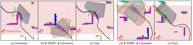
Figure 3: Simulation results with goal position $\left[10\ 10\ 1\right]^{\top}$ and disturbances $\left[3\ 3\ 0\right]^{\top}$ in Section VI-B. The black line is the trajectory, the blue line is the reference trajectory, the red zone is the area where the external forces are applied to the quadrotor, the shaded polytope is the safety constraint, and the gold star is the goal position. (a) [30] collides with obstacles and often has poor safety rate; (b) [31] collides with obstacles due to latency of R-NMPC; (d) R-NMPC in [31] has longer flight time and trajectory length since it aims to guarantee safety against worst-case disturbances over a lookahead horizon; (c) & (e) Our method achieves collision avoidance while having better performance in flight time, trajectory length, and tracking error.

Simulation Setup. The quadrotor dynamics and the Gazebo simulation environment and system architecture are as follows:

VI-B1 Quadrotor Dynamics

$$\dot{\bm{p}} =\bm{v},\quad m\dot{\bm{v}} =m\bm{g}+\bm{f}+\bm{f}_{w},$$ (9)

$$\dot{\bm{R}} =\bm{R}\left[\bm{\omega}\right]^{\wedge},\quad \mathcal{J}\dot{\bm{\omega}} =-\bm{\omega}\times\mathcal{J}\bm{\omega}+\bm{\tau},\vspace{-3mm}$$ (10)

where $\bm{p}\in\mathbb{R}^{3}$ and $\mathbf{v}\in\mathbb{R}^{3}$ are position and velocity in the iniertial frame, $\bm{R}\in\mathrm{SO}(3)$ is the attitude rotation matrix, $\bm{\omega}\in\mathbb{R}^{3}$ is the body angular velocity, $m$ is the quadrotor mass, $\mathcal{J}$ is the inertia matrix of the quadrotor, the wedge operator ${}^{\wedge}:\mathbb{R}^{3}\rightarrow\mathfrak{s}\mathfrak{e}(3)$ is the skew-symmetric mapping, $\mathbf{g}$ is the gravity vector, $\bm{f}=\bm{R}\left[0\ 0\ T\right]^{\top}\in\mathbb{R}^{3}$ and $\bm{\tau}\in\mathbb{R}^{3}$ are the total thrust and body torques from four rotors, $T$ is the thrust from four rotors along the $z-$axis of the body frame, and $\bm{f}_{w}\in\mathbb{R}^{3}$ is the unknown external force.

VI-B2 Gazebo Environment and System Architecture

The Gazebo environment is illustrated in Figure 1. We simulate the quadrotor using RotorS [47]. The quadrotor is equipped with an Inertial Measurement Unit (IMU) and a camera.

The system architecture is illustrated in Figure 2. We use occupancy grid mapping [48] for mapping the unknown environment. The external force estimator using VID-Fusion [49] provides an estimate $\tilde{\bm{f}}_{w}$ of $\bm{f}_{w}$. The path planning module using EGO-Planner [50] provides a sequence of desired position $\bm{p}_{r}$, velocity $\bm{v}_{r}$, acceleration $\dot{\bm{v}}_{r}$, yaw angle, and yaw rate. We generate polytopic safety constraints using DecompROS [51], which uses maps of inflated obstacles to account for a quadrotor’s size. We use OSQP solver [52] for the projection step.

VI-B3 Control Design

Similar to [53, 54], we focus on the translational dynamics in eq. 9 and use Algorithm 1 to design the desired force $\bm{f}_{d}$, which is then decomposed into the desired rotation matrix $\bm{R}_{d}$ and the desired thrust $T_{d}$ given a desired yaw angle. To this end, we assume that a nonlinear attitude controller, e.g., [30], generates the desired torque such that the desired rotation matrix $\bm{R}_{d}$ is tracked.

The desired force takes the form of $\bm{f}_{d}=-k_{p}\bm{e}_{\bm{p}}-k_{v}\bm{e}_{\bm{v}}+m\dot{\bm{v}}_{r}-m\bm{g}-\tilde{\bm{f}}_{w}+m\bm{a}$, where $\bm{e}_{\bm{p}}$ and $\bm{e}_{\bm{v}}$ are tracking errors in position and velocity, $k_{p}$ and $k_{v}$ are control gains, $\tilde{\bm{f}}_{w}$ is the estimation of the external force, and $\bm{a}$ is the control input learned by Algorithm 1 using loss function $250\|\bm{e}_{\bm{p}}\|^{2}+10\|\bm{e}_{\bm{v}}\|^{2}$. We use the second-order Runge-Kutta (RK2) method [55] for discretization.

VI-B4 Source of Non-Stochastic Noise

Since a stochastic model for the estimation error $\|\tilde{\bm{f}}_{w}-\bm{f}_{w}\|$ is generally unknown, we assume the bound $\|\tilde{\bm{f}}_{w}-\bm{f}_{w}\|\,\leq 0.1$; i.e., $f_{w}=\tilde{f}_{w}+\mathbf{n}$, where $\|\mathbf{n}\|\,\leq 0.1$, and $\mathbf{n}$ plays the role of non-stochastic noise in the quadrotor dynamics.

VI-B5 Benchmark Experiment Setup

We consider that the quadrotor is tasked to fly to prescribed goal positions in the presence of unknown constant external forces that simulate sudden wind gusts; the goal positions and the direction of the wind gusts are specified in Table II. Particularly, the external forces are applied to the quadrotor as long as its $x$ and $y$ positions are within the box $(x,y)\in[1,\ 10]\times[-10,\ 10]$. We use as performance metrics the flight time, trajectory length, tracking error, computational time, and safety rate.

Compared Algorithms. We compare Algorithm 1 with [30] and [31]. [30] is a geometric controller that tracks a desired path based on the feedback of the tracking errors. [31] uses a robust nonlinear model predictive control (R-NMPC) as a planner with the translational dynamics in eq. 9 and a simplified attitude dynamics model. Particularly, given the external force estimation from VID-Fusion, the desired acceleration $\dot{\bm{v}}_{r}$ provided by R-NMPC in [31] compensates the external force $\bm{f}_{w}$. With the R-NMPC working as a low-frequency outer-loop controller, [31] then use [30] as a high-frequency inner-loop tracking controller.

Results. The results are given in Table II and Figure 3. Algorithm 1 demonstrates improved performance to [30, 31] in terms of the flight time, trajectory length, tracking error, and safety rate. Moreover, our method is able to achieve $100\%$ safety rate across all tested scenarios, in contrast to [30, 31]. The reasons that [30, 31] do not achieve $100\%$ safety rate appear to be the following: [30] has higher tracking error under unknown forces (Figure 3​ a) and R-NMPC in [31] results in a collision due to latency (Figure 3​ b). Under varying disturbances, the high tracking error of [30] leads to the worst performance in flight time and trajectory length. Additionally, R-NMPC in [31] has longer flight time and trajectory length than Algorithm 1 since it aims to guarantee safety against worst-case disturbances over a lookahead horizon (Figure 3​ d).

VII Conclusion

Summary. We studied the problem of Safe Non-Stochastic Control for Control-Affine Systems (1), and provided the Safe-OGD algorithm. Safe-OGD guarantees safety and bounded dynamic regret against any time-varying control policy (Theorem 1). Safe-OGD is near-optimal for classical online convex optimization and optimal control problems: (i) when the domain of optimization is time-invariant, Safe-OGD’s performance bound reduces to the bound of the OGD algorithm for online convex optimization, which is near-optimal [27]; and (ii) when also the optimal clairvoyant control policy is time–invariant, Safe-OGD can learn it asymptotically, implying, for example, that Safe-OGD will converge to the optimal linear state-feedback controller if applied to the classical LQG problem. We evaluated our algorithm in simulated scenarios of an inverted pendulum aiming to stay inverted, and a quadrotor flying in an unknown cluttered environment (Section VI). We observed that our method demonstrated better performance, guaranteeing safety, whereas state-of-the-art methods, such as the iLQR [6] and R-NMPC [31] did not.

Future work. We will investigate the regret bound of the Safe-OGD algorithm under unknown stochastic noise, providing Best-of-Both-Worlds guarantees in mixed stochastic and non-stochastic environments.

References

- [1] E. Ackerman, “Amazon promises package delivery by drone: Is it for real?” IEEE Spectrum, Web, 2013.
- [2] J. Chen, T. Liu, and S. Shen, “Tracking a moving target in cluttered environments using a quadrotor,” in 2016 IEEE/RSJ International Conference on Intelligent Robots and Systems (IROS). IEEE, 2016, pp. 446–453.
- [3] A. Rivera, A. Villalobos, J. C. N. Monje, J. A. G. Mariñas, and C. M. Oppus, “Post-disaster rescue facility: Human detection and geolocation using aerial drones,” in IEEE 10 Conference, 2016, pp. 384–386.
- [4] J. B. Rawlings, D. Q. Mayne, and M. Diehl, Model predictive control: Theory, computation, and design. Nob Hill Publishing, 2017, vol. 2.
- [5] F. Borrelli, A. Bemporad, and M. Morari, Predictive control for linear and hybrid systems. Cambridge University Press, 2017.
- [6] J. Chen, W. Zhan, and M. Tomizuka, “Constrained iterative lqr for on-road autonomous driving motion planning,” in 2017 IEEE 20th International conference on intelligent transportation systems (ITSC). IEEE, 2017, pp. 1–7.
- [7] R. K. Cosner, P. Culbertson, A. J. Taylor, and A. D. Ames, “Robust safety under stochastic uncertainty with discrete-time control barrier functions,” arXiv preprint arXiv:2302.07469, 2023.
- [8] O. Faltinsen, Sea loads on ships and offshore structures. Cambridge University Press, 1993, vol. 1.
- [9] K. J. Åström, Introduction to stochastic control theory. Courier Corporation, 2012.
- [10] W. Khalil and E. Dombre, Modeling identification and control of robots. CRC Press, 2002.
- [11] D. Q. Mayne, M. M. Seron, and S. Raković, “Robust model predictive control of constrained linear systems with bounded disturbances,” Automatica, vol. 41, no. 2, pp. 219–224, 2005.
- [12] G. Goel and B. Hassibi, “Regret-optimal control in dynamic environments,” arXiv preprint:2010.10473, 2020.
- [13] O. Sabag, G. Goel, S. Lale, and B. Hassibi, “Regret-optimal full-information control,” arXiv preprint:2105.01244, 2021.
- [14] A. Martin, L. Furieri, F. Dörfler, J. Lygeros, and G. Ferrari-Trecate, “Safe control with minimal regret,” in Learning for Dynamics and Control Conference (L4DC), 2022, pp. 726–738.
- [15] A. Didier, J. Sieber, and M. N. Zeilinger, “A system level approach to regret optimal control,” IEEE Control Systems Letters (L-CSS), 2022.
- [16] H. Zhou and V. Tzoumas, “Safe perception-based control with minimal worst-case dynamic regret,” arXiv preprint:2208.08929, 2022.
- [17] N. Agarwal, B. Bullins, E. Hazan, S. Kakade, and K. Singh, “Online control with adversarial disturbances,” in International Conference on Machine Learning (ICML), 2019, pp. 111–119.
- [18] M. Simchowitz, K. Singh, and E. Hazan, “Improper learning for non-stochastic control,” in Conference on Learning Theory (COLT), 2020, pp. 3320–3436.
- [19] Y. Li, S. Das, and N. Li, “Online optimal control with affine constraints,” in AAAI Conference on Artificial Intelligence (AAAI), vol. 35, no. 10, 2021, pp. 8527–8537.
- [20] P. Zhao, Y.-H. Yan, Y.-X. Wang, and Z.-H. Zhou, “Non-stationary online learning with memory and non-stochastic control,” arXiv preprint arXiv:2102.03758, 2021.
- [21] N. M. Boffi, S. Tu, and J.-J. E. Slotine, “Regret bounds for adaptive nonlinear control,” in Learning for Dynamics and Control. PMLR, 2021, pp. 471–483.
- [22] H. Zhou, Z. Xu, and V. Tzoumas, “Efficient online learning with memory via frank-wolfe optimization: Algorithms with bounded dynamic regret and applications to control,” arXiv preprint arXiv:2301.00497, 2023.
- [23] H. Zhou and V. Tzoumas, “Safe non-stochastic control of linear dynamical systems,” arXiv preprint arXiv:2308.12395, 2023.
- [24] E. Hazan et al., “Introduction to online convex optimization,” Foundations and Trends in Optimization, vol. 2, no. 3-4, pp. 157–325, 2016.
- [25] A. D. Ames, J. W. Grizzle, and P. Tabuada, “Control barrier function based quadratic programs with application to adaptive cruise control,” in 53rd IEEE Conference on Decision and Control. IEEE, 2014, pp. 6271–6278.
- [26] D. Xue, Y. Chen, and D. P. Atherton, Linear feedback control: analysis and design with MATLAB. SIAM, 2007.
- [27] M. Zinkevich, “Online convex programming and generalized infinitesimal gradient ascent,” in Interna. Conf. on Machine Learning (ICML), 2003, pp. 928–936.
- [28] D. Silver, G. Lever, N. Heess, T. Degris, D. Wierstra, and M. Riedmiller, “Deterministic policy gradient algorithms,” in International conference on machine learning. Pmlr, 2014, pp. 387–395.
- [29] T. P. Lillicrap, J. J. Hunt, A. Pritzel, N. Heess, T. Erez, Y. Tassa, D. Silver, and D. Wierstra, “Continuous control with deep reinforcement learning,” arXiv preprint arXiv:1509.02971, 2015.
- [30] T. Lee, M. Leok, and N. H. McClamroch, “Geometric tracking control of a quadrotor uav on se (3),” in 49th IEEE conference on decision and control (CDC). IEEE, 2010, pp. 5420–5425.
- [31] Y. Wu, Z. Ding, C. Xu, and F. Gao, “External forces resilient safe motion planning for quadrotor,” IEEE Robotics and Automation Letters, vol. 6, no. 4, pp. 8506–8513, 2021.
- [32] B. Hassibi, A. H. Sayed, and T. Kailath, Indefinite-Quadratic estimation and control: A unified approach to and theories, 1999.
- [33] S. Bansal, M. Chen, S. Herbert, and C. J. Tomlin, “Hamilton-jacobi reachability: A brief overview and recent advances,” in 2017 IEEE 56th Annual Conference on Decision and Control (CDC). IEEE, 2017, pp. 2242–2253.
- [34] J. N. Maidens, S. Kaynama, I. M. Mitchell, M. M. Oishi, and G. A. Dumont, “Lagrangian methods for approximating the viability kernel in high-dimensional systems,” Automatica, vol. 49, no. 7, pp. 2017–2029, 2013.
- [35] J. Darbon and S. Osher, “Algorithms for overcoming the curse of dimensionality for certain hamilton–jacobi equations arising in control theory and elsewhere,” Research in the Mathematical Sciences, vol. 3, no. 1, p. 19, 2016.
- [36] S. Herbert, J. J. Choi, S. Sanjeev, M. Gibson, K. Sreenath, and C. J. Tomlin, “Scalable learning of safety guarantees for autonomous systems using hamilton-jacobi reachability,” in 2021 IEEE International Conference on Robotics and Automation (ICRA). IEEE, 2021, pp. 5914–5920.
- [37] A. D. Ames, X. Xu, J. W. Grizzle, and P. Tabuada, “Control barrier function based quadratic programs for safety critical systems,” IEEE Transactions on Automatic Control, vol. 62, no. 8, pp. 3861–3876, 2016.
- [38] A. Agrawal and K. Sreenath, “Discrete control barrier functions for safety-critical control of discrete systems with application to bipedal robot navigation.” in Robotics: Science and Systems, vol. 13. Cambridge, MA, USA, 2017.
- [39] J. Zeng, B. Zhang, and K. Sreenath, “Safety-critical model predictive control with discrete-time control barrier function,” in 2021 American Control Conference (ACC). IEEE, 2021, pp. 3882–3889.
- [40] A. Clark, “Control barrier functions for complete and incomplete information stochastic systems,” in 2019 American Control Conference (ACC). IEEE, 2019, pp. 2928–2935.
- [41] M. Jankovic, “Robust control barrier functions for constrained stabilization of nonlinear systems,” Automatica, vol. 96, pp. 359–367, 2018.
- [42] H. K. Khalil, Nonlinear control. Pearson New York, 2015, vol. 406.
- [43] S. Sun, A. Romero, P. Foehn, E. Kaufmann, and D. Scaramuzza, “A comparative study of nonlinear mpc and differential-flatness-based control for quadrotor agile flight,” IEEE Transactions on Robotics, vol. 38, no. 6, pp. 3357–3373, 2022.
- [44] L. Zhang, S. Lu, and Z.-H. Zhou, “Adaptive online learning in dynamic environments,” Advances in Neural Information Processing Systems (NeurIPS), vol. 31, 2018.
- [45] S. Diamond and S. Boyd, “CVXPY: A Python-embedded modeling language for convex optimization,” Journal of Machine Learning Research, vol. 17, no. 83, pp. 1–5, 2016.
- [46] A. Raffin, A. Hill, A. Gleave, A. Kanervisto, M. Ernestus, and N. Dormann, “Stable-baselines3: Reliable reinforcement learning implementations,” Journal of Machine Learning Research, vol. 22, no. 268, pp. 1–8, 2021.
- [47] F. Furrer, M. Burri, M. Achtelik, and R. Siegwart, Robot Operating System (ROS): The Complete Reference (Volume 1). Cham: Springer International Publishing, 2016, ch. RotorS—A Modular Gazebo MAV Simulator Framework, pp. 595–625. [Online]. Available: http://dx.doi.org/10.1007/978-3-319-26054-9_23
- [48] S. Thrun, “Probabilistic robotics,” Communications of the ACM, vol. 45, no. 3, pp. 52–57, 2002.
- [49] Z. Ding, T. Yang, K. Zhang, C. Xu, and F. Gao, “Vid-fusion: Robust visual-inertial-dynamics odometry for accurate external force estimation,” in 2021 IEEE International Conference on Robotics and Automation (ICRA). IEEE, 2021, pp. 14 469–14 475.
- [50] X. Zhou, J. Zhu, H. Zhou, C. Xu, and F. Gao, “Ego-swarm: A fully autonomous and decentralized quadrotor swarm system in cluttered environments,” in 2021 IEEE international conference on robotics and automation (ICRA). IEEE, 2021, pp. 4101–4107.
- [51] S. Liu, “Mrsl decomputil library.” [Online]. Available: https://github.com/sikang/DecompROS
- [52] B. Stellato, G. Banjac, P. Goulart, A. Bemporad, and S. Boyd, “OSQP: an operator splitting solver for quadratic programs,” Mathematical Programming Computation, vol. 12, no. 4, pp. 637–672, 2020.
- [53] D. Morgan, S.-J. Chung, and F. Y. Hadaegh, “Swarm assignment and trajectory optimization using variable-swarm, distributed auction assignment and model predictive control,” in AIAA guidance, navigation, and control conference, 2015, p. 0599.
- [54] G. Shi, X. Shi, M. O’Connell, R. Yu, K. Azizzadenesheli, A. Anandkumar, Y. Yue, and S.-J. Chung, “Neural lander: Stable drone landing control using learned dynamics,” in International Conference on Robotics and Automation (ICRA), 2019, pp. 9784–9790.
- [55] P. E. Kloeden, E. Platen, P. E. Kloeden, and E. Platen, Stochastic differential equations. Springer, 1992.
- [56] A. Ben-Tal, L. El Ghaoui, and A. Nemirovski, Robust optimization. Princeton university press, 2009, vol. 28.