Axisymmetric hybrid Vlasov equilibria with applications to tokamak plasmas

Abstract

We derive axisymmetric equilibrium equations in the context of the hybrid Vlasov model with kinetic ions and massless fluid electrons, assuming isothermal electrons and deformed Maxwellian distribution functions for the kinetic ions. The equilibrium system comprises a Grad-Shafranov partial differential equation and an integral equation. These equations can be utilized to calculate the equilibrium magnetic field and ion distribution function, respectively, for given particle density or given ion and electron toroidal current density profiles. The resulting solutions describe states characterized by toroidal plasma rotation and toroidal electric current density. Additionally, due to the presence of fluid electrons, these equilibria also exhibit a poloidal current density component. This is in contrast to the fully kinetic Vlasov model, where axisymmetric Jeans equilibria can only accommodate toroidal currents and flows, given the absence of a third integral of the microscopic motion.

1 Introduction

Hybrid Vlasov models play an important role in examining the complex behavior of multiscale plasmas that feature both a fluid bulk and energetic particle populations not amenable to fluid descriptions. One specific branch of hybrid models that has received significant attention, primarily for studying phenomena in ion inertial scales such as turbulence and collisionless reconnection, focuses on electron-ion plasmas where electrons are treated as a fluid while ions are treated kinetically (e.g. [1, 2, 3, 4, 5, 6, 7, 8]). In our recent work ([9]), we employed such a hybrid model, featuring massless isothermal electrons and kinetic ions, to investigate one-dimensional Alfvén-BGK (Bernstein-Greene-Kruskal) modes as stationary solutions to the model equations. We demonstrated that the one-dimensional equilibrium equations constitute a Hamiltonian system for a pseudoparticle, which can exhibit integrable or chaotic orbits, depending on the form of the distribution function. A natural extension of this work would be the construction of 2D-equilibria which can be used as reference states for studying reconnection, instabilities and wave propagation, or even macroscopic equilibria of fusion plasmas.

Plasmas in fusion devices like the tokamak, are enriched with significant populations of energetic particles. It is thus expected that the distribution of those particles in the physical and the velocity space might affect macroscopic equilibrium and stability properties. For this reason hybrid models have also found applications in the description of multiscale dynamics of tokamak plasmas (e.g. [10, 11, 12]). However, despite the utility of hybrid and kinetic descriptions for investigating dynamical processes, there has been limited progress in constructing self-consistent equilibria within the framework of thes models. One important limitation arises from the absence of a third particle constant of motion in the full-orbit Vlasov description. Such an invariant would be crucial for constructing equilibria with characteristics relevant to tokamaks. Efforts to build such equilibria using a fully kinetic Vlasov description for both ions and electrons have been undertaken in [13, 14]. Nevertheless, due to the presence of only one momentum integral of motion for each particle species, specifically the particle toroidal angular momentum, these equilibria exhibit only toroidal current density and plasma rotation. In contrast, the magnetohydrodynamic (MHD) fluid description of toroidal plasma equilibrium can accommodate both toroidal and poloidal currents. Hence, although more fundamental, the kinetic approach appears to have limitations in describing certain classes of equilibria compared to MHD.

To combine the advantages of both descriptions, we turn to the hybrid model mentioned earlier. Even though it lacks a poloidal particle momentum invariant, it can describe equilibria featuring both toroidal and poloidal current densities, thanks to the fluid treatment of electrons, which carry the poloidal current component. It is important to note though that a limitation of the present model for a realistic description of fusion plasmas, is that it treats the entire ion population using the Vlasov equation. This is not the most efficient and effective approach, since there is also a thermal ion component and multiple ion species; thus further model improvements are required. The present model description serves as an initial step toward the development of improved models that will incorporate multi-fluid-kinetic descriptions, as exemplified in [15].

The rest of the paper is structured as follows: in Section 2 we present the hybrid equilibrium model and in Section 3 the axisymmetric equilibrium formulation is developed. In Section 4 we numerically construct particular tokamak-pertinent equilibria presenting various equilibrium characteristics and we conclude by summarising the results in Section 5.

2 The hybrid model

The initial hybrid-Vlasov equilibrium system employed in [9], consists of a Vlasov equation for kinetic ions, a generalized Ohm’s law derived from the electron momentum equation, the Maxwell equations, and an equation of state for the fluid electrons:

$$\bm{v}\cdot\nabla f+\frac{e}{m}\left(\textbf{E}+\bm{v}\times\textbf{B}\right)\cdot\nabla_{\bm{v}}f=0\,,$$ (1)

$$\textbf{E}=-\frac{n}{n_{e}}\textbf{u}\times{\mathbf{B}}+\frac{{\mathbf{J}}\times{\mathbf{B}}}{en_{e}}-\frac{\nabla P_{e}}{en_{e}}\,,$$ (2)

$$\textbf{E}=-\nabla\Phi\,,\quad\nabla\times{\mathbf{B}}=\mu_{0}{\mathbf{J}}\,,$$ (3)

$$\quad\nabla\cdot{\mathbf{B}}=0\,,\quad\nabla\cdot\textbf{E}=e(n-n_{e})\,,$$ (4)

$$P_{e}=n_{e}k_{B}T_{e}\,,$$ (5)

where

$$n({\mathbf{x}},t)=\int d^{3}v\,f({\mathbf{x}},\bm{v},t)\,,$$ (6)

$${\mathbf{u}}({\mathbf{x}},t)=n^{-1}\int d^{3}v\,\bm{v}f({\mathbf{x}},\bm{v},t)\,.$$ (7)

Note that the ion-kinetic contribution to the current density is given by

$$\textbf{J}_{k}=\int d^{3}v\,\bm{v}f\,,$$ (8)

and thus the first term in the right hand side of (2) can be expressed as $-\textbf{J}_{k}\times\textbf{B}/(en_{e})$.

In addition to (1)–(5), an energy equation is needed to determine $T_{e}$. Alternatively, it can be assumed that the electrons are isothermal, i.e. $T_{e}$ is constant throughout the entire plasma volume, or it can vary with the magnetic flux function $\psi$ if we consider isothermal magnetic surfaces, i.e., $T_{e}=T_{e}(\psi)$. An alternative to (5) would be an isentropic closure of the form $P_{e}=cn_{e}^{\gamma}\,,$ or even anisotropic electron pressure under appropriate conditions for the different components of the electron pressure tensor. Here we consider isothermal electrons $T_{e}=T_{e0}=const.$

Let us now write the system (1)–(5) in nondimensional form upon indtroducing the following dimensionless quantities

$$\tilde{x}=\frac{x}{R_{0}}\,,\quad\tilde{\bm{v}}=\frac{\bm{v}}{d_{i}v_{A}}\,,$$

$$\tilde{n}_{e}=\frac{n_{e}}{n_{0}}\,,\quad\tilde{f}=d_{i}^{3}v_{A}^{3}f/n_{0}\,,$$

$$\tilde{\textbf{E}}=\frac{\textbf{E}}{d_{i}v_{A}B_{0}}\,,\quad\tilde{\textbf{B}}=\frac{\textbf{B}}{B_{0}}\,,$$

$$\tilde{\textbf{J}}_{k}=\frac{\textbf{J}_{k}}{en_{0}d_{i}v_{A}}\,,\quad\tilde{P}_{e}=\frac{P_{e}}{mn_{0}d_{i}^{2}v_{A}^{2}}\,,$$ (9)

where $R_{0}$ and $B_{0}$ are the characteristic length and magnetic field modulus, respectively. Additionally,

$$v_{A}=\frac{B_{0}}{\sqrt{\mu_{0}mn_{0}}}\,,\quad\Omega=\frac{eB_{0}}{m}\,,$$ (10)

are the Alfvén speed and the ion cyclotron frequency, respectively and

$$d_{i}=\frac{\ell_{i}}{R_{0}}\,,\quad\ell_{i}=\sqrt{\frac{m}{\mu_{0}n_{0}e^{2}}}\,,$$ (11)

is the nondimensional ion skin depth which is typically of the order $10^{-2}$ in fusion devices. Notice that apart from nondimensionalizing various physical quantities, we’ve also scaled the nondimensional velocity by a factor of $d_{i}^{-1}$. The rationale behind this scaling will be clarified in a subsequent explanation. What is important to stress here, is that with careful implementation of this scaling process, there are no inconsistencies in the nondimensionalization of the equations and the recovery of physical units in the final results. In view of (9) the hybrid equilibrium system then can be written in the following nondimensional form:

$$\bm{v}\cdot\nabla f+d_{i}^{-2}\left(\textbf{E}+\bm{v}\times\textbf{B}\right)\cdot\nabla_{v}f=0\,,$$ (12)

$$-\nabla\Phi=\frac{1}{n_{e}}\left[\left(\nabla\times\textbf{B}-\textbf{J}_{k}\right)-d_{i}^{2}\nabla P_{e}\right]\,,$$ (13)

$$\textbf{E}=-\nabla\Phi\,,\quad\nabla\times\textbf{B}=\textbf{J}\,,$$ (14)

$$\nabla\cdot\textbf{B}=0\,,\quad d_{i}^{2}\beta_{A}^{2}\nabla\cdot E=(n-n_{e})\,,$$ (15)

$$P_{e}=\kappa n_{e}\,,$$ (16)

where

$$\kappa:=\frac{k_{B}T_{e0}}{d_{i}^{2}mv_{A}^{2}}\,.$$ (17)

and $\beta_{A}^{2}=v_{A}^{2}/c^{2}$. Taking the limit $\beta_{A}^{2}\rightarrow 0$ we obtain the quasineutrality condition $n_{e}=n$, which will be applied in the subsequent analysis.

In Section 3, we will investigate two equilibrium scenarios: one with cold electrons ($\kappa=0$) and the other with thermal electrons ($\kappa=1$). We opted for the scaled nondimensional particle velocity $\tilde{v}=v/(d_{i}v_{A})$ with the goal of attaining tokamak-relevant temperatures making the convenient choice $\kappa=1$. It can be verified through (17) and using an Alfvén speed calculated from tokamak-relevant values for the density and the magnetic field, that $\kappa=1$ corresponds to $T_{e0}\sim 10^{8}\,K$.

As a closing note for this section, it is worth highlighting that taking into account (16) and the quasineutrality condition $n_{e}=n$, Ohm’s law (13) can be expressed as follows:

$$-\nabla\Phi=\frac{1}{n}\left(\nabla\times\textbf{B}-\textbf{J}_{k}\right)\times\textbf{B}-\nabla ln\left(n^{d_{i}^{2}\kappa}\right)\,.$$ (18)

3 Axisymmetric equilibrium formulation

We consider a plasma configuration with axial symmetry with respect to a fixed axis, where all quantities depend on the coordinates $r,z$ of a cylindrical coordinate system $(r,\phi,z)$. Note that $z$ coincides with the axis of symmetry. In this case the divergence-free magnetic field can be written in terms of two scalar functions $I$ and $\psi$ as follows:

$${\mathbf{B}}=I\nabla\phi+\nabla\psi(r,z)\times\nabla\phi\,,$$ (19)

while the corresponding current density is

$${\mathbf{J}}=\nabla\times{\mathbf{B}}=-\Delta^{*}\psi\nabla\phi+\nabla I\times\nabla\phi\,,$$ (20)

where $\Delta^{*}$ is the Shafranov operator given by

$$\Delta^{*}=r\frac{\partial}{\partial r}\left(\frac{1}{r}\frac{\partial}{\partial r}\right)+\frac{\partial^{2}}{\partial z^{2}}\,.$$ (21)

Next we will consider the three components of (18) along the magnetic field, along the $\hat{\phi}$ direction and along the $\nabla\psi$ direction. From the B projection we readily obtain

$$\textbf{B}\cdot\nabla\left[\Phi-ln\left(n^{d_{i}^{2}\kappa}\right)\right]=0\,,$$ (22)

thus

$$\Phi-ln\left(n^{d_{i}^{2}\kappa}\right)\eqqcolon G(\psi)\,,$$ (23)

where $G(\psi)$ is an arbitrary function. From this equation we can solve for $n$ to find

$$n=exp\left[\frac{\Phi-G(\psi)}{d_{i}^{2}\kappa}\right]\,.$$ (24)

In the case $G(\psi)=const.$ we recover the Boltzmann distribution. Next, to take the $\nabla\phi$ and $\nabla\psi$ projections we need first to determine the direction of $\textbf{J}_{k}$.

According to Jeans’ theorem [16, 17], distribution functions of the form $f=f(C_{1},C_{2},...)$, where $C_{i}$ are particle constants of motion, are solutions to the Vlasov equation (12). In the absence of collisions, the particle energy $H$ is itself a first integral of motion. In nondimensional form $H$ reads:

$$\tilde{H}=\frac{v^{2}}{2}+d_{i}^{-2}\Phi\,,$$ (25)

where $\tilde{H}=H/(d_{i}^{2}mv_{A}^{2})$. Additionally, in the presence of axial symmetry a second constant of motion is the particle toroidal angular momentum

$$\tilde{p}_{\phi}=rv_{\phi}+rA_{\phi}=rv_{\phi}+d_{i}^{-2}\psi\,,$$ (26)

where $\tilde{p}_{\phi}=p_{\phi}/(mR_{0}d_{i}v_{A})$. It remains an open question whether and under what conditions, additional, approximate constants of motion exist within the framework of full-orbit Vlasov description (see [18] and references therein for a discussion on the existence of a third integral of motion in axisymmetric potentials). In certain scenarios, it may be pertinent to consider adiabatic constants, such as the magnetic moment $\mu$ as explored in [19]. It is worth noting that in the context of the hybrid model and the present analysis, some assumptions made in [19], such as $p_{\phi}\approx\psi$, can be justified due to the presence of the significant $d_{i}^{-2}$ factor, especially in systems like the magnetosphere. However, in this paper, which focuses on laboratory plasmas, we will not adopt this assumption. Instead, we will follow the approach outlined in [9] and [20], considering a distribution function in the form of:

$$f=exp(-H)g(p_{\phi})=exp\left[-\frac{v_{r}^{2}+v_{z}^{2}+v_{\phi}^{2}}{2}-\Phi(r,z)\right]g(p_{\phi})\,,$$ (27)

or

$$f=exp\left[-\frac{v_{r}^{2}+v_{z}^{2}}{2}-\frac{(p_{\phi}-\psi)^{2}}{2r^{2}}-\Phi(r,z)\right]g(p_{\phi})\,.$$

Note that the tildes have been omitted in $H$ and $p_{\phi}$ for convenience. For such a distribution function the kinetic current density (8) will have only a $\phi$ component. This is because $v_{r}f$ and $v_{z}f$ are odd functions with respect to $v_{r}$ and $v_{z}$ respectively, while the integration over these variables go from $-\infty$ to $+\infty$. Therefore

$$\textbf{J}_{k}=rJ_{k\phi}\nabla\phi\,,$$

and as a result

$$\textbf{J}_{k\phi}\times\textbf{B}=\frac{J_{k\phi}}{r}\nabla\psi\,.$$ (28)

Substituting (19), (20), (24) and (28) into (18) we obtain

$$-n\nabla\Phi=-\frac{\Delta^{*}\psi}{r^{2}}\nabla\psi-\frac{I}{r^{2}}\nabla I+[I,\psi]\nabla\phi-\frac{J_{k\phi}}{r}\nabla\psi-n\nabla\Phi+nG^{\prime}(\psi)\nabla\psi\,,$$ (29)

where $[a,b]\coloneqq(\nabla a\times\nabla b)\cdot\nabla\phi$. It is now trivial to see that from the $\nabla\phi$ projection of (29), we obtain

$$[I,\psi]=0\,,\quad\text{i.e.\,}\quad I=I(\psi)\,.$$ (30)

Finally, the $\nabla\psi$ projection yields

$$\Delta^{*}\psi+II^{\prime}(\psi)+r^{2}\mathcal{Z}(r,\psi)=0\,,$$ (31)

where

$$\mathcal{Z}(r,\psi):=\frac{1}{r}\int d^{3}v\,v_{\phi}f-G^{\prime}(\psi)\int d^{3}v\,f\,.$$

Equation (31) is a Grad-Shafranov (GS) equation determining the magnetic field through the flux function $\psi$ in axisymmetric hybrid Vlasov equilibria. Let us now work out the velocity space integrals in (31). The particle density is

$$n=\int d^{3}v\,f=\frac{e^{-\Phi/d_{i}^{2}}}{r}\int_{-\infty}^{+\infty}dv_{r}\int_{-\infty}^{+\infty}dv_{z}\int_{-\infty}^{+\infty}dp_{\phi}\,e^{-\frac{v_{r}^{2}}{2}-\frac{v_{z}^{2}}{2}-\frac{(p_{\phi}-\psi/d_{i}^{2})^{2}}{2r^{2}}}g(p_{\phi})$$

$$=\frac{2\pi e^{-\Phi/d_{i}^{2}}}{r}\int_{-\infty}^{\infty}dp_{\phi}\,e^{-\frac{(p_{\phi}-\psi/d_{i}^{2})^{2}}{2r^{2}}}g(p_{\phi})\,.$$ (32)

We have shown that $\Phi=ln(n^{d_{i}^{2}\kappa})+G(\psi)$, therefore

$$n=\left[\frac{2\pi e^{-G(\psi)/d_{i}^{2}}}{r}\int_{-\infty}^{+\infty}dp_{\phi}\,e^{-\frac{(p_{\phi}-\psi/d_{i}^{2})^{2}}{2r^{2}}}g(p_{\phi})\right]^{\frac{1}{\kappa+1}}\,.$$ (33)

Similarly, for the toroidal component of the kinetic current density we find

$$J_{k\phi}=2\pi e^{-G(\psi)/d_{i}^{2}}\left[\frac{2\pi e^{-G(\psi)/d_{i}^{2}}}{r}\int_{-\infty}^{+\infty}dp_{\phi}\,e^{-\frac{(p_{\phi}-\psi/d_{i}^{2})^{2}}{2r^{2}}}g(p_{\phi})\right]^{-\frac{\kappa}{\kappa+1}}\times$$

$$\times\int_{-\infty}^{+\infty}dp_{\phi}\,\frac{(p_{\phi}-\psi/d_{i}^{2})}{r^{2}}e^{-\frac{(p_{\phi}-\psi/d_{i}^{2})^{2}}{2r^{2}}}g(p_{\phi})\,.$$ (34)

Therefore, the current density depends on two arbitrary functions, i.e. $G(\psi)$ and $g(p_{\phi})$. The latter function that determines the ion distribution function, can either be specified a-priori, together with $G(\psi)$ and then the GS equation (31) can be solved to determine $\psi$, or can be identified by fixing $J_{k\phi}$ and $G(\psi)$. Following the formalism of [9] we can show that the function $\mathcal{Z}(r,\psi)$ can be derived by a “pseudopotential” function $V(r,\psi)$ which takes the form

$$V(\psi,r)=d_{i}^{2}(\kappa+1)\left[\frac{2\pi e^{-G(\psi)/d_{i}^{2}}}{r}\int_{-\infty}^{+\infty}dp_{\phi}\,e^{-\frac{(p_{\phi}-\psi/d_{i}^{2})^{2}}{2r^{2}}}g(p_{\phi})\right]^{\frac{1}{\kappa+1}}=d_{i}^{2}(\kappa+1)n\,.$$ (35)

We can easily verify that

$$\mathcal{Z}=\frac{\partial V}{\partial r}\,,$$

thus, the Grad-Shafranov equation can be written in the familiar form

$$\Delta^{*}\psi+II^{\prime}(\psi)+r^{2}\frac{\partial V}{\partial\psi}=0\,.$$ (36)

Note that equation (36) is reminiscent of the MHD GS equation with toroidal flow [21], where an effective pressure function associated with the thermodynamic pressure and the plasma flow, appears instead of $V(r,\psi)$.

To solve Eq. (36) we can specify $V(\psi,r)$ to be a known mathematical function or it can be inferred by experimental data from the particle density $n$ or the toroidal current density profile. Note that the particle density and the total toroidal current density can be expressed in terms of $V$ as follows

$$n=\frac{V}{d_{i}^{2}(\kappa+1)}\,,\quad J_{\phi}=\frac{II^{\prime}}{r}+r\frac{\partial V}{\partial\psi}.$$ (37)

Also note that that the electron contribution to $J_{\phi}$ is given by

$$J_{e\phi}=\frac{II^{\prime}}{r}-rnG^{\prime}(\psi)\,.$$ (38)

Knowing $V$ enables the solution of the partial differential equation (36) to determine $\psi$ and of the integral equation (35) to determine $g(p_{\phi})$.

Now, we demonstrate that when the product $V^{\kappa+1}e^{G(\psi)/d_{i}^{2}}$ can be expressed as a power series expansion of $\psi$, it becomes possible to determine the function $g(p_{\phi})$ in terms of Hermite polynomials. To illustrate this, let us invoke that Hermite polynomials $H_{n}(x)$ serve as coefficients in the following power series expansion [22]

$$e^{-(x-y)^{2}/2}=\sum_{n=0}^{\infty}\frac{e^{-x^{2}/2}}{n!}H_{n}\left(\frac{x}{\sqrt{2}}\right)\left(\frac{y}{\sqrt{2}}\right)^{n}\,,$$ (39)

therefore (35) can be written as

$$\left[\frac{V}{d_{i}^{2}(\kappa+1)}\right]^{\kappa+1}e^{G(\psi)/d_{i}^{2}}=\sum_{n}\frac{2\pi}{n!}\int_{-\infty}^{+\infty}d\zeta\,e^{-\zeta^{2}/2}H_{n}\left(\frac{\zeta}{\sqrt{2}}\right)\left(\frac{\psi}{d_{i}^{2}\sqrt{2}r}\right)^{n}g(r\zeta)\,,$$ (40)

where $\zeta:=p_{\phi}/r$. As Hermite polynomials form a complete orthogonal basis we can expand $g(r\zeta)$ as

$$g(r\zeta)=\sum_{m}c_{m}H_{m}\left(\frac{r\zeta}{\sqrt{2}}\right)\,.$$ (41)

We now make use of the multiplication theorem for Hermite polynomials [23]

$$H_{m}(\gamma x)=\sum_{\ell=0}^{\lfloor m/2\rfloor}\gamma^{m-2\ell}(\gamma^{2}-1)^{\ell}\frac{m!}{\ell!(m-2\ell)!}H_{m-2\ell}(x)\,,\quad\forall\gamma\in\mathbb{R}\,,$$ (42)

to write

$$g(r\zeta)=\sum_{m}\sum_{\ell=0}^{\lfloor m/2\rfloor}c_{m}\frac{m!}{\ell!(m-2\ell)!}r^{m-2\ell}(r^{2}-1)^{\ell}H_{m-2\ell}\left(\frac{\zeta}{\sqrt{2}}\right)\,.$$ (43)

Substituting (43), the right hand side (rhs) of (40) becomes

$$\sum_{m,n}\sum_{\ell=0}^{\lfloor m/2\rfloor}\frac{2\pi}{n!}c_{m}\frac{m!}{\ell!(m-2\ell)!}r^{m-2\ell}(r^{2}-1)^{\ell}\left(\frac{\psi}{d_{i}^{2}\sqrt{2}r}\right)^{n}\times$$

$$\times\int_{-\infty}^{+\infty}d\zeta\,e^{-\zeta^{2}/2}H_{n}\left(\frac{\zeta}{\sqrt{2}}\right)H_{m-2\ell}\left(\frac{\zeta}{\sqrt{2}}\right)\,.$$ (44)

Further, exploiting the orthogonality condition

$$\int_{-\infty}^{+\infty}dx\,H_{n}(x)H_{m}(x)e^{-x^{2}}=\sqrt{\pi}2^{n}n!\delta_{mn}\,,$$ (45)

we can see that Eq. (40) with rhs given by (44), becomes

$$\left[\frac{V}{d_{i}^{2}(\kappa+1)}\right]^{\kappa+1}e^{G(\psi)/d_{i}^{2}}=\sum_{m}\sum_{\ell=0}^{\lfloor m/2\rfloor}2^{m-2\ell+1}\pi^{3/2}c_{m}\frac{m!}{\ell!(m-2\ell)!}(r^{2}-1)^{\ell}\left(\frac{\psi}{d_{i}^{2}\sqrt{2}}\right)^{m-2\ell}\,.$$ (46)

Our aim is to solve (46) for $c_{m}$ in order to determine $g(p_{\phi})$ as an expansion of orthogonal Hermite polynomials (see Eq. (41)). This is possible if the left hand side (lhs) of (46) can be expressed as a power series expansion. In this work we consider the special case

$$\left[\frac{V}{d_{i}^{2}(\kappa+1)}\right]^{\kappa+1}e^{G(\psi)/d_{i}^{2}}=V_{0}(r)+V_{1}(r)\psi+V_{2}(r)\psi^{2}\,,$$ (47)

and deal with two classes of equilibria corresponding to cold electrons with $\kappa=1$ and thermal electrons with $\kappa=1$.

By equations (47) and (46) we see that

$$V_{0}+V_{1}\psi+V_{2}\psi^{2}=c_{0}2\pi^{3/2}+c_{1}\frac{(2\pi)^{3/2}}{d_{i}^{2}}\psi+c_{2}\frac{4\pi^{3/2}}{d_{i}^{4}}\psi^{2}+c_{2}4\pi^{3/2}(r^{2}-1)\,,$$ (48)

and therefore the coefficients $c_{0}$, $c_{1}$ and $c_{2}$ are

$$c_{0} = \frac{V_{0}(r)}{2\pi^{3/2}}-2c_{2}(r^{2}-1)\,,$$ (49)

$$c_{1} = \frac{d_{i}^{2}V_{1}}{2\pi^{3/2}}\,,$$ (50)

$$c_{2} = \frac{d_{i}^{4}V_{2}}{4\pi^{3/2}}\,.$$ (51)

In order for $c_{0},c_{1},c_{2}$ to be constants we should select $V_{1}=const.$ $V_{2}=const.$ and

$$V_{0}(r)=C_{0}+d_{i}^{4}V_{2}(r^{2}-1)\,,$$

where $C_{0}$ is a constant. Therefore, the ion distribution function in both the cold and thermal electron limits reads as follows

$$f(H,p_{\phi})=\left[c_{0}+\sqrt{2}c_{1}p_{\phi}+c_{2}(2p_{\phi}^{2}-2)\right]e^{-H}\,.$$ (52)

To ensure the positivity of the distribution function (52) it suffices to require $c_{0}+\sqrt{2}c_{1}p_{\phi}+c_{2}(2p_{\phi}^{2}-2)>0$, $\forall p_{\phi}$, which holds true for

$$c_{0}>\frac{c_{1}^{2}-8c_{2}^{2}}{4c_{2}}\,,\quad c_{2}>0\,.$$

4 Tokamak equilibria

To fully define the plasma equilibria we further need to specify the free functions $I(\psi)$ and $G(\psi)$. In this work we adopt

$$I(\psi) = (I_{0}+I_{1}\psi+I_{2}\psi^{2})e^{-(\psi-\psi_{a})^{2}/\eta}\,,$$ (53)

$$G(\psi) = \alpha(\psi-\psi_{a})^{2}\,.$$ (54)

Here, $I_{0}$, $I_{1}$, $I_{2}$, $\eta$, and $\alpha$ are constants, and $\psi_{a}$ represents the value of the flux function $\psi$ at the magnetic axis, corresponding to an elliptic O-point of $\psi$ where the magnetic field is purely toroidal.

We address the fixed-boundary equilibrium problem within a tokamak-relevant, D-shaped computational domain denoted as $\mathcal{D}$. In this context, we solve the Grad-Shafranov equation (36) while specifying $V$ as

$$V=d_{i}^{2}e^{-G(\psi)/d_{i}^{2}}\left[V_{0}(r)+V_{1}\psi+V_{2}\psi^{2}\right]\,,$$ (55)

$$V=2d_{i}^{2}\left\{e^{-G(\psi)/d_{i}^{2}}\left[V_{0}(r)+V_{1}\psi+V_{2}\psi^{2}\right]\right\}^{1/2}\,,$$ (56)

for the $\kappa=0$ and $\kappa=1$ cases, respectively. The boundary condition is of Dirichlet type given by $\psi|_{\partial\mathcal{D}}=0$. For cold electrons the Grad-Shafranov equation (36) takes the familiar form

$$\Delta^{*}\psi+II^{\prime}(\psi)+d_{i}^{2}e^{-G/d_{i}^{2}}\left[\left(V_{1}+2V_{2}\psi\right)-\frac{G^{\prime}(\psi)}{d_{i}^{2}}\left(C_{0}-d_{i}^{4}V_{2}+V_{1}\psi+V_{2}\psi^{2}\right)\right]r^{2}$$

$$-d_{i}^{2}V_{2}e^{-G/d_{i}^{2}}G^{\prime}(\psi)r^{4}=0\,.$$ (57)

Note that a Grad-Shafranov equation of similar structure describes axisymmetric equilibria with incompressible flows of arbitrary direction, as shown in [24]. In the MHD context the $r^{4}$ term is associated with the non-parallel component of the flow.

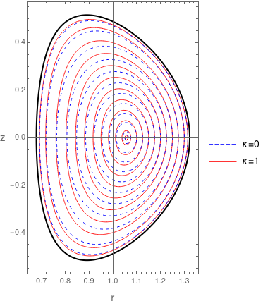
Figure 1: Magnetic surfaces of an equilibrium with cold electrons (blue dashed lines) and an equilibrium with thermal electrons (red solid lines).

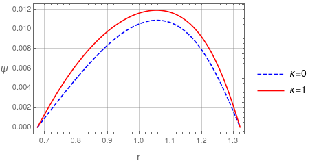
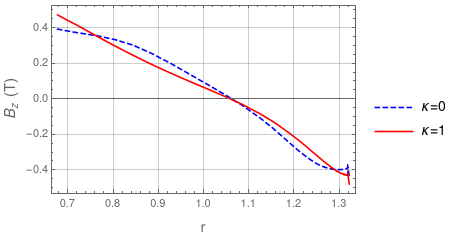
Figure 2: Variation of the flux functions $\psi$ (left) and the $z$ component of the magnetic field (right) along the $r$ axis on the equatorial plane $z=0$. The dashed blue lines correspond to the cold electron equilibrium and the red solid lines correspond to thermal electrons.

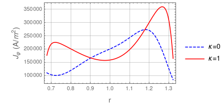
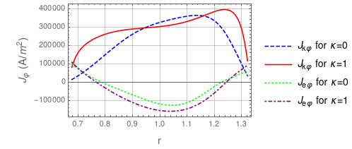
Figure 3: The toroidal current density profiles for the two equilibrium classes. The total current density profile is displayed in the left panel, while in the right panel the electron and the ion kinetic contributions are drawn separately.

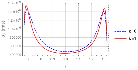
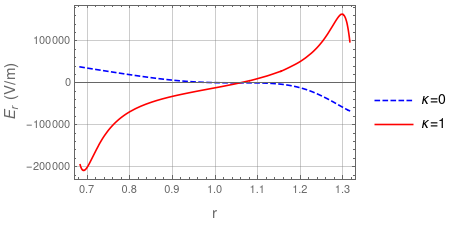
Figure 4: The toroidal rotation velocity profile (left) and the corresponding profile of the $r$ component of the electric field on $z=0$.

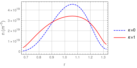
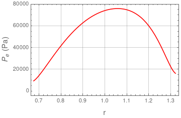
Figure 5: Particle density profiles for $\kappa=0$ and $\kappa=1$ (left panel) and the electron pressure for $\kappa=1$ (right panel).

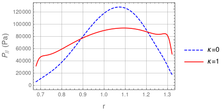
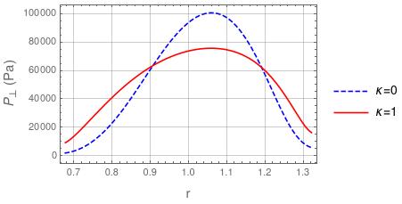
Figure 6: Variation of the parallel (left panel) and perpendicular (right panel) components of the ion pressure tensor along $r$ axis on $z=0$ for both $\kappa=0$ and $\kappa=1$.

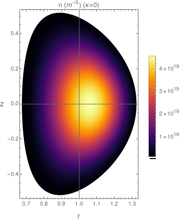
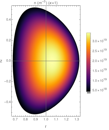
Figure 7: Two dimensional density plots for the particle densities in $\kappa=0$ (left panel) and $\kappa=1$ (right panel) case.

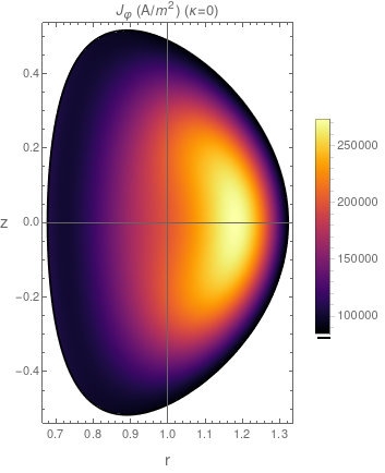
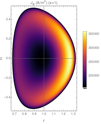
Figure 8: Variation of $J_{\phi}$ component on the $r-z$ plane for $\kappa=0$ (left) and $\kappa=1$ (right).

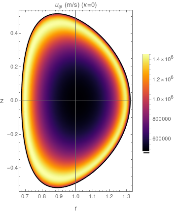
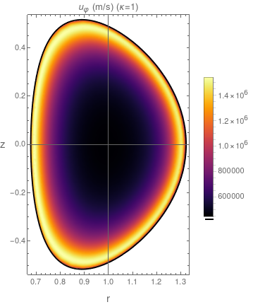
Figure 9: The variation of the toroidal rotation velocity $u_{\phi}$ on the plane $r-z$, for cold (left) and thermal electrons (right).

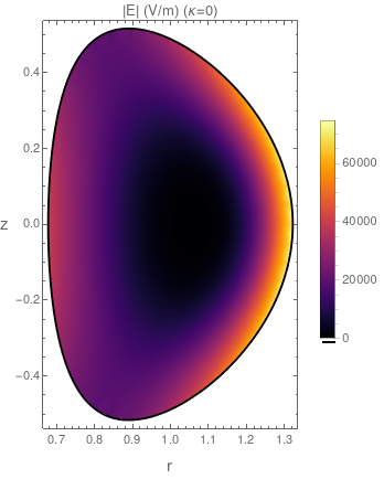
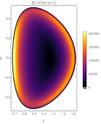
Figure 10: The variation of the electric field magnitude $|\textbf{E}|$ on the plane $r-z$, for cold (left) and thermal electrons (right).

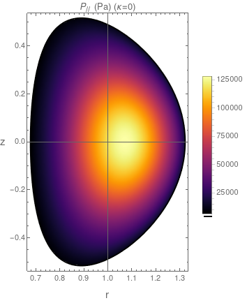
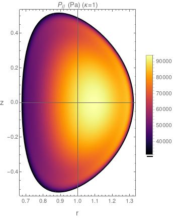
Figure 11: The parallel component ($P_{\parallel}$) of the ion pressure tensor for cold (left panel) and thermal (right panel) electrons.

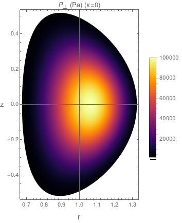
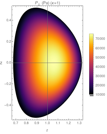
Figure 12: The perpendicular component ($P_{\perp}$) of the ion pressure tensor for cold (left panel) and thermal (right panel) electrons.

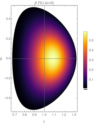
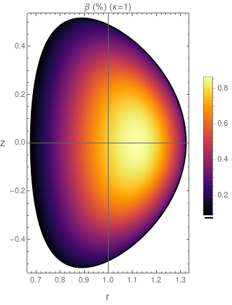
Figure 13: Plasma $\beta$ calculated using (58) for the case $\kappa=0$ (left) and the case $\kappa=1$ (right).

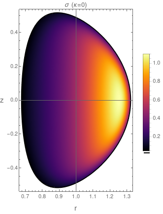
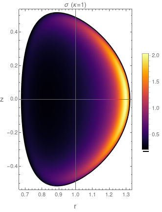
Figure 14: The anisotropy function $\sigma$, calculated by (63) for $\kappa=0$ (left) and $\kappa=1$ (right).

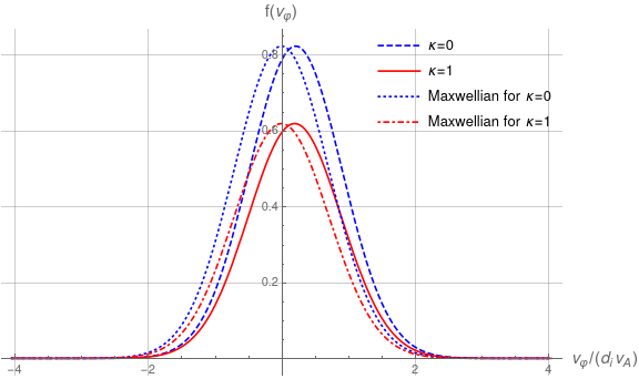
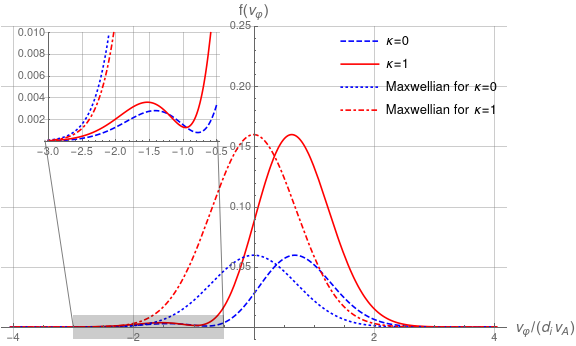
Figure 15: Variation of the ion distribution function $f$ computed by (52) with $v_{\phi}$, at two different locations: at the magnetic axis (left) and at an edge point with coordinates ($r=1.3,z=0.0$) (right).

We solve both boundary value problems, corresponding to $\kappa=0$ and $\kappa=1$, using the Finite Element Method (FEM), which is conveniently implemented in Mathematica. The boundary $\partial\mathcal{D}$ of the computational domain $\mathcal{D}$ is defined as a polygon with a large number of vertices. The vertex coordinates can be boundary points extracted by some parametric formula or by experimental data. The boundary is characterized by an inverse aspect ratio $\epsilon=0.32$, triangularity $\delta=0.34$ and elongation equal to $1.6$. The characteristic values of length, magnetic field and number density used for unit recovery are, respectively $R_{0}=6.2\,m$, $B_{0}=5\,T$ and $n_{0}=2.1\times 10^{19}$. The algorithm performs several iterations as the position of the magnetic axis has to be found because it is required for determining the function $G=\alpha(\psi-\psi_{a})^{2}$, until the convergence criterion $max(|\psi_{new}-\psi_{old}|)<tol$ is satisfied. For our calculations we have set $tol=10^{-7}$.

The contours of constant $\psi$ (magnetic surfaces) for both equilibria are shown in Fig. 1. These equilibria are calculated by solving (36) with the ansatz (53) for $I(\psi)$. In the case of cold electrons, the function $V$ is given by (55), while for thermal electrons, $V$ is specified by (56). The values of the free parameters in the functions $I$ and $V$ are identical for both cases. For the specific examples presented here, we have chosen $I_{0}=0.5$, $I_{1}=10^{-1}$, $I_{2}=-14$, $V_{1}=15$, $V_{2}=1.02\times 10^{4}$, $\alpha=7.5$, and $\eta=10$.

The characteristics of the equilibrium can be deduced from Figures 2 to 6, which display variations of various physical quantities of interest along the $r$ axis on the $z=0$ plane. Two-dimensional density plots of the same quantities are presented in Figures 7 to 14. Notably, the particle density in both equilibria does not vanish at the boundary (Figures 5 and 7), implying that this equilibrium model is suitable for describing internal plasma regions bounded by a closed magnetic surface which defines the computational domain and does not coincide with the actual plasma boundary.

Additionally, we observe that the toroidal plasma rotation velocity profile exhibits a hollow shape with significant flow shear and radial electric field ($E_{r}$) in the plasma edge (Figs. 4, 9, and 10). Such edge sheared flows have been associated with the reduction of radial turbulent transport and the transition to high (H) confinement modes in large tokamaks (e.g., [25, 26]). Moreover, the toroidal current density profile for the $\kappa=1$ equilibrium shows a reduction in the central region of the plasma (Figs. 3, 8).

We also examine the parallel and perpendicular components of the ion pressure tensor, as presented in Figures 11 and 12. The steps for obtaining $P_{\parallel}$ and $P_{\perp}$ can be found in Appendix A. In Fig. 6, we provide profiles of these components, along with the electron pressure profile in the case of $\kappa=1$. Notably, the $P_{\parallel}$ component of the ion pressure tensor forms a pedestal in the thermal electron case. As a consequence, the effective pressure defined as $(P_{\parallel}+P_{\perp})/2$ also forms a pedestal due to the $P_{\parallel}$ contribution.

In addition to the previously mentioned physical quantities, we calculate two figures of merit for both cold and thermal electron equilibria: the plasma $\beta$ and the anisotropy function $\sigma$ (defined in Appendix A, Eq. (63)). In nondimensional form the expression for calculating the plasma $\beta$ is:

$$\beta=d_{i}^{2}\frac{P_{e}+\langle P\rangle}{B^{2}}\,,$$ (58)

where $\langle P\rangle:=P_{rr}+P_{zz}+P_{\phi\phi}$ with $P_{rr},P_{zz},P_{\phi\phi}$ being the diagonal components of the pressure tensor (see Appendix A). The presence of the $d_{i}^{2}$ factor arises owing to the specific scaling we have adopted for the normalized pressure in Eqs. (9). Figures 13 and 14 illustrate that the plasma $\beta$ ranges from approximately $0.5-1.0\%$ and increases from the plasma boundary towards the core, while the ion pressure anisotropy is more pronounced on the low-field side of the configuration.

We conclude our presentation of equilibrium results with Fig. 15, which illustrates the variation of ion distribution functions as a function of the toroidal particle component $v_{\phi}$, for both $\kappa=0$ and $\kappa=1$ cases at two distinct locations: the magnetic axis $(r_{ax},z_{az})$ and an edge point with coordinates $(r=1.3,z=0.0)$. In both cases, the dependence on $v_{r}$ and $v_{z}$ has been eliminated by integrating the distribution functions over the $v_{r}-v_{z}$ plane. The two distribution functions are presented alongside the corresponding normalized Maxwellian distributions $f_{0}e^{-v_{\phi}^{2}}$, where $f_{0}$ is an appropriate normalization constant. In both cases, the distributions exhibit a shift towards positive $v_{\phi}$, resulting in finite macroscopic toroidal flows. At the edge point $(1.3,0)$, where the toroidal flow appears to reach a maximum, the distributions significantly deviates from the Maxwellian, displaying a bump-on-tail form. The bump arises from ions rotating in the opposite direction of the macroscopic flow.

5 Summary

In this work, we have presented the axisymmetric equilibrium formulation of the hybrid Vlasov equilibrium model introduced in [9], featuring massless electrons and kinetic ions. We derived a general form of the Grad-Shafranov equation and outlined a method for determining ion distribution functions in terms of Hermite polynomials based on the knowledge of the total and the electron current density profile. Our formulation allowed us to solve the equilibrium problem for specific choices of the arbitrary functions involved in the Grad-Shafranov equation. The results demonstrate the model’s capability to describe plasmas with geometric and profile characteristics relevant to tokamaks. Notably, these equilibria exhibit some features reminiscent of H-mode phenomenology, including strongly sheared edge flows and significant edge radial electric fields. Building upon these results, more refined descriptions of plasma equilibria with kinetic effects stemming from kinetic particle populations are possible. Thus, future research will focus on improving the model to incorporate realistic electron temperature distribution and fluid ion components. An intriguing open question is whether this equilibrium model can be derived through a Hamiltonian energy-Casimir (EC) variational principle, as explored in [15, 27]. Identifying the complete set of Casimir invariants of the dynamical system is crucial for such a variational formulation of the equilibrium problem and for establishing stability criteria within the Hamiltonian framework. Note that, in general, there are not enough Casimirs to recover all the possible classes of equilibria due to rank changing of the Poisson operator (see [28]). However, instead of the EC variational principle, one can apply an alternative Hamiltonian variational method that recovers all equilibria upon utilizing dynamically accessible variations [28].

Appendix A Calculation of the ion pressure tensor components

The ion pressure tensor is defined by

$$\textbf{P}=\int d^{3}v\,(\bm{v}-\textbf{u})(\bm{v}-\textbf{u})f\,,$$ (59)

where u is calculated by (7). In our case $\textbf{u}=u_{\phi}\hat{\phi}$. Selecting the $(v_{r},v_{z},v_{\phi})$ basis in the velocity space we calculate below the following diagonal pressure components $P_{rr},P_{zz},P_{\phi}$. Note that the non-diagonal components $P_{rz}=P_{r\phi}=P_{z\phi}=0$ vanish owing to the fact that $f$ is an even function of the velocity components $v_{r}$, $v_{z}$. The diagonal elements are calculated as follows

$$P_{rr} = \int d^{3}v\,v_{r}^{2}f\,,$$ (60)

$$P_{zz} = \int d^{3}v\,v_{z}^{2}f\,,$$ (61)

$$P_{\phi\phi} = \int d^{3}v\,(v_{\phi}-u_{\phi})^{2}f\,.$$ (62)

An average value of the ion pressure is given by $\langle P\rangle=Tr(P_{ij})/3$.

It is evident that $P_{rr}=P_{zz}$ and since the non-diagonal components are zero, the ion pressure tensor is gyrotropic and can be written in the form

$$\textbf{P}=\sigma\textbf{B}\textbf{B}+P_{\perp}\textbf{I}\,,$$ (63)

where

$$\sigma\coloneqq d_{i}^{2}\frac{P_{\parallel}-P_{\perp}}{B^{2}}\,,$$

is an anisotropy function. Note that the factor $d_{i}^{2}$ appears due to the specific scaling of the particle velocity adopted in (9). The parallel and the perpendicular to B components of the pressure tensor can be calculated by the following relations

$$P_{\parallel} = \frac{\textbf{P}\bm{:}\textbf{B}\textbf{B}}{B^{2}}=\frac{P_{ij}B_{i}B_{j}}{B^{2}}\,,$$ (64)

$$P_{\perp} = \frac{1}{2}\textbf{P}\bm{:}\left(\textbf{I}-\frac{\textbf{B}\textbf{B}}{B^{2}}\right)=\frac{1}{2}P_{ij}\left(\delta_{ij}-\frac{B_{i}B_{j}}{B^{2}}\right)\,.$$ (65)

References

- Valentini et al. [2007] F. Valentini, P. Trávníček, F. Califano, P. Hellinger, and A. Mangeney. A hybrid-Vlasov model based on the current advance method for the simulation of collisionless magnetized plasma. Journal of Computational Physics, 225(1):753–770, 2007. ISSN 0021-9991. doi: https://doi.org/10.1016/j.jcp.2007.01.001. URL https://doi.org/10.1016/j.jcp.2007.01.001.
- Servidio et al. [2012] S. Servidio, F. Valentini, F. Califano, and P. Veltri. Local kinetic effects in two-dimensional plasma turbulence. Phys. Rev. Lett., 108:045001, Jan 2012. doi: 10.1103/PhysRevLett.108.045001. URL https://link.aps.org/doi/10.1103/PhysRevLett.108.045001.
- Servidio et al. [2015] S. Servidio, F. Valentini, D. Perrone, A. Greco, F. Califano, W. H. Matthaeus, and P. Veltri. A kinetic model of plasma turbulence. Journal of Plasma Physics, 81:325810107, 2015. doi: 10.1017/S0022377814000841. URL https://doi.org/10.1017/S0022377814000841.
- Cerri et al. [2016] S. S. Cerri, F. Califano, F. Jenko, D. Told, and F. Rincon. Subproton scale cascades in solar wind turbulence: driven hybrid-kinetic simulations. The Astrophysical Journal, 822(1):L12, apr 2016. doi: 10.3847/2041-8205/822/1/l12. URL https://doi.org/10.3847/2041-8205/822/1/l12.
- González et al. [2020] C. A. González, A. Tenerani, M. Velli, and P. Hellinger. The role of parametric instabilities in turbulence generation and proton heating: Hybrid simulations of parallel-propagating alfvén waves. The Astrophysical Journal, 904(1):81, nov 2020. doi: 10.3847/1538-4357/abbccd. URL https://dx.doi.org/10.3847/1538-4357/abbccd.
- Tenerani et al. [2023] Anna Tenerani, Carlos González, Nikos Sioulas, Chen Shi, and Marco Velli. Dispersive and kinetic effects on kinked Alfvén wave packets: A comparative study with fluid and hybrid models. Physics of Plasmas, 30(3):032101, 2023. doi: 10.1063/5.0134726. URL https://doi.org/10.1063/5.0134726.
- Winske et al. [2003] Dan Winske, Lin Yin, Nick Omidi, Homa Karimabadi, and Kevin Quest. Hybrid Simulation Codes: Past, Present and Future—A Tutorial, pages 136–165. Springer Berlin Heidelberg, Berlin, Heidelberg, 2003. ISBN 978-3-540-36530-3. doi: 10.1007/3-540-36530-3_8. URL https://doi.org/10.1007/3-540-36530-3_8.
- Le et al. [2016] A. Le, W. Daughton, H. Karimabadi, and J. Egedal. Hybrid simulations of magnetic reconnection with kinetic ions and fluid electron pressure anisotropy. Physics of Plasmas, 23(3):032114, 2016. doi: 10.1063/1.4943893. URL https://doi.org/10.1063/1.4943893.
- Kaltsas et al. [2023] Dimitrios A. Kaltsas, Philip J. Morrison, and George N. Throumoulopoulos. Chaotic and integrable magnetic fields in one-dimensional hybrid Vlasov–Maxwell equilibria. Journal of Plasma Physics, 89(4):905890403, 2023. doi: 10.1017/S0022377823000557. URL https://doi.org/10.1017/S0022377823000557.
- Park et al. [1999] W. Park, E. V. Belova, G. Y. Fu, X. Z. Tang, H. R. Strauss, and L. E. Sugiyama. Plasma simulation studies using multilevel physics models. Physics of Plasmas, 6(5):1796–1803, 1999. doi: 10.1063/1.873437. URL https://doi.org/10.1063/1.873437.
- Todo [2016] Y Todo. Multi-phase hybrid simulation of energetic particle driven magnetohydrodynamic instabilities in tokamak plasmas. New Journal of Physics, 18(11):115005, 2016. doi: 10.1088/1367-2630/18/11/115005. URL https://doi.org/10.1088/1367-2630/18/11/115005.
- Todo et al. [2021] Y Todo, M Sato, Hao Wang, M Idouakass, and R Seki. Magnetohydrodynamic hybrid simulation model with kinetic thermal ions and energetic particles. Plasma Physics and Controlled Fusion, 63(7):075018, jun 2021. doi: 10.1088/1361-6587/ac0162. URL https://dx.doi.org/10.1088/1361-6587/ac0162.
- Tasso and Throumoulopoulos [2014] H. Tasso and G. Throumoulopoulos. Tokamak-like Vlasov equilibria. Eur. Phys. J. D, 68:175, 2014. doi: https://doi.org/10.1140/epjd/e2014-50007-9. URL https://doi.org/10.1140/epjd/e2014-50007-9.
- Kuiroukidis et al. [2015] Ap Kuiroukidis, G. N. Throumoulopoulos, and H. Tasso. Vlasov tokamak equilibria with sheared toroidal flow and anisotropic pressure. Physics of Plasmas, 22(8):082505, 2015. doi: 10.1063/1.4928111. URL https://doi.org/10.1063/1.4928111.
- Kaltsas et al. [2021] D.A. Kaltsas, G.N. Throumoulopoulos, and P.J. Morrison. Hamiltonian kinetic-Hall magnetohydrodynamics with fluid and kinetic ions in the current and pressure coupling schemes. Journal of Plasma Physics, 87(5):835870502, 2021. doi: https://doi.org/10.1017/S0022377821000994. URL https://doi.org/10.1017/S0022377821000994.
- Jeans [1915] J. H. Jeans. On the Theory of Star-Streaming and the Structure of the Universe. Monthly Notices of the Royal Astronomical Society, 76(2):70–84, 12 1915. ISSN 0035-8711. doi: 10.1093/mnras/76.2.70. URL https://doi.org/10.1093/mnras/76.2.70.
- Lynden-Bell [1962] D. Lynden-Bell. Stellar Dynamics: Only Isolating Integrals Should be used in Jeans’ Theorem. Monthly Notices of the Royal Astronomical Society, 124(1):1–9, 01 1962. ISSN 0035-8711. doi: 10.1093/mnras/124.1.1. URL https://doi.org/10.1093/mnras/124.1.1.
- Efthymiopoulos et al. [2007] Christos Efthymiopoulos, Nikos Voglis, and C. Kalapotharakos. Special Features of Galactic Dynamics, pages 297–389. Springer Berlin Heidelberg, Berlin, Heidelberg, 2007. ISBN 978-3-540-72984-6. doi: 10.1007/978-3-540-72984-6_11. URL https://doi.org/10.1007/978-3-540-72984-6_11.
- Aibara et al. [2021] H. Aibara, Z. Yoshida, and K. Shirahata. Kinetic construction of the high-beta anisotropic-pressure equilibrium in the magnetosphere. Physics of Plasmas, 28(12):122301, 2021. doi: 10.1063/5.0069971. URL https://doi.org/10.1063/5.0069971.
- Allanson et al. [2016] O. Allanson, T. Neukirch, S. Troscheit, and F. Wilson. From one-dimensional fields to Vlasov equilibria: theory and application of hermite polynomials. Journal of Plasma Physics, 82(3):905820306, 2016. doi: 10.1017/S0022377816000519. URL https://doi.org/10.1017/S0022377816000519.
- Maschke and Perrin [1980] E K Maschke and H Perrin. Exact solutions of the stationary MHD equations for a rotating toroidal plasma. Plasma Physics, 22(6):579, jun 1980. doi: 10.1088/0032-1028/22/6/007. URL https://dx.doi.org/10.1088/0032-1028/22/6/007.
- Morse and Feshbach [1953] P. M. Morse and H. Feshbach. Methods of Theoretical Physics. McGraw-Hill, New York, 1953.
- Chaggara and Koepf [2007] Hamza Chaggara and Wolfram Koepf. Duplication coefficients via generating functions. Complex Variables and Elliptic Equations, 52(6):537–549, 2007. doi: 10.1080/17476930701236967. URL https://doi.org/10.1080/17476930701236967.
- Tasso and Throumoulopoulos [1998] H. Tasso and G. N. Throumoulopoulos. Axisymmetric ideal magnetohydrodynamic equilibria with incompressible flows. Physics of Plasmas, 5(6):2378–2383, 1998. doi: 10.1063/1.872912. URL https://doi.org/10.1063/1.872912.
- Burrell [2020] K. H. Burrell. Role of sheared E × B flow in self-organized, improved confinement states in magnetized plasmas. Physics of Plasmas, 27(6):060501, 2020. doi: https://doi.org/10.1063/1.5142734. URL https://doi.org/10.1063/1.5142734.
- Plank et al. [2022] U Plank, R M McDermott, G Birkenmeier, N Bonanomi, M Cavedon, G D Conway, T Eich, M Griener, O Grover, P A Schneider, M Willensdorfer, and the ASDEX Upgrade Team. Overview of L- to H-mode transition experiments at ASDEX upgrade. Plasma Physics and Controlled Fusion, 65(1):014001, dec 2022. doi: 10.1088/1361-6587/aca35b. URL https://dx.doi.org/10.1088/1361-6587/aca35b.
- Tronci et al. [2015] C. Tronci, E. Tassi, and P. J Morrison. Energy-casimir stability of hybrid Vlasov-MHD models. Journal of Physics A: Mathematical and Theoretical, 48(18):185501, apr 2015. doi: 10.1088/1751-8113/48/18/185501. URL https://iopscience.iop.org/article/10.1088/1751-8113/48/18/185501.
- Morrison [1998] P. J. Morrison. Hamiltonian description of the ideal fluid. Rev. Mod. Phys., 70:467–521, Apr 1998. doi: 10.1103/RevModPhys.70.467. URL https://link.aps.org/doi/10.1103/RevModPhys.70.467.