Surface plasmon-polaritons in graphene, embedded into medium with gain and losses

Abstract

The paper deals with the theoretical consideration of surface plasmon-polaritons in the graphene monolayer, embedded into dielectric with spatially separated gain and losses. It is demonstrated, that presence of gain and losses in the system leads to the formation of additional mode of graphene surface plasmon-polaritons, which does not have its counterpart in the conservative system. When the gain and losses are mutually balanced, the position of exceptional point – transition point between unbroken and broken $\mathcal{PT}$-symmetry – can be effectively tuned by graphene’s doping. In the case of unbalanced gain and losses the spectrum of surface plasmon-polaritons contains spectral singularity, whose frequency is also adjustable through the electrostatic gating of graphene.

Keywords graphene  $\cdot$ surface plasmon-polariton  $\cdot$ $\mathcal{PT}$-symmetry

1 Introduction

The physical systems, which involve both media with gain and media with losses exhibits one specific and counter-intuitive property: being in general non-Hermitian systems, under certain relation between gain and losses they can possess real spectrum (similar to Hermitian system). In the particular situation of $\mathcal{PT}$-symmetry [1] the gain and losses are perfectly balanced and the coordinate-dependent complex external potential $V\left(\mathbf{r}\right)$ is characterized by the property $V\left(\mathbf{r}\right)=V^{*}\left(-\mathbf{r}\right)$ [here star stands for the complex conjugation]. In the $\mathcal{PT}$-symmetric structure the spectrum is real (this situation is called unbroken $\mathcal{PT}$-symmetry) for gain/loss values below the certain threshold and is complex for gain/loss values above this threshold. The later situation is referred as broken $\mathcal{PT}$-symmetry and is characterized by the presence of two modes: one is growing and another is decaying. Although initially the conception of $\mathcal{PT}$-symmetry was introduced in the quantum mechanical formalism, nowadays it is unclear, whether some real quantum object described by the $\mathcal{PT}$-symmetric Hamiltonian can be found in nature. Nevertheless, experimentally the existence of $\mathcal{PT}$-symmetry was demonstrated in a variety of other fields, namely mechanical systems [2], acoustics [3], LRC circuits[4], coupled optical waveguides [5, 6, 7], or whispering-gallery resonators [8].

Certain similarity between Maxwell and Schrödinger equation leads to the possibility of the realization of $\mathcal{PT}$-symmetry in optical systems, where spatial distribution of dielectric permittivity obeys the relation $\varepsilon\left(\mathbf{r}\right)=\varepsilon^{*}\left(-\mathbf{r}\right)$. At the same time $\mathcal{PT}$-symmetric optical systems exhibit a series of unusual properties like nonreciprocal (nonsymmetrical) wave propagation [6], negative refraction [9, 10, 11], simultaneous lasing and coherent perfect absorption[12, 13, 14], unidirectional visibility [15, 16, 17].

Optical systems, which operation principle is based on bulk electromagnetic waves, possess certain limit in the miniaturization of their components, called diffraction limit. One of possible ways to overcome this diffraction limit is to build photonic systems, which operate on surface waves (namely, surface plasmon-polaritons) instead of bulk ones. Nevertheless, surface plasmon-polaritons in noble metals has relatively short lifetime due to high losses. In connection with this, using the $\mathcal{PT}$-symmetry in plasmonics[18, 19, 20, 21, 22, 23, 24] can be very promising, because it could compensate losses in the noble metals and originate lossless propagation of surface plasmon-polaritons. Another possibility to reduce losses in plasmonics is to use a two-dimensional carbon material graphene. Surface plasmon-polaritons sustained by the graphene exhibit both longer lifetime and degree of localization [25, 26], if compared to surface plasmon-polaritons in noble metals. At the same time, graphene’s conductivity can be dynamically varied through the electrostatic gating[27], last fact allows to tune dynamically the wavelength [28, 29, 30, 31, 32] of graphene surface plasmon-polaritons (GSPPs) as well as realize tunable sensor [33] or plasmonic modulator [34, 35]. Along with this, gated graphene embedded into the $\mathcal{PT}$-symmetric structures allows to achieve dynamical tunability of losses[36]. At the same time an optical pumping of the graphene allows the realization of gain [37, 38, 39] and, as a consequence, amplification of GSPPs[40, 41]. Pumped graphene, being implemented into the lossy medium, allows the realization of the $\mathcal{PT}$-symmetry for a series of purposes like sensing [42], waveguiding [43, 44], or diffraction grating [45].

Nevertheless, the $\mathcal{PT}$–symmetric structures are not unique systems with gain or losses, which are characterized by real spectrum. For example, a finite slab of optical gainy medium at certain discrete frequencies possesses real spectrum[46]. These frequencies, called spectral singularities, behave like a zero-width resonances. Also a special relation between unbalanced gain and loss can give rise to the generalized $\mathcal{PT}$-symmetry[47], which exhibits the same properties as its $\mathcal{PT}$-symmetric counterpart. Along with this, systems with unbalanced gain and losses can exhibit a series of properties like perfect absorption [48], directional coupling[49] and lossless waveguiding[50].

In this paper we consider GSPPs in graphene monolayer, cladded between two dielectric layers: one is with gain, another with loss. We show, that when lossless graphene is imbedded into $\mathcal{PT}$-symmetric dielectric surrounding, the positions of the exceptional points in GSPP can be effectively tuned by changing graphene’s Fermi energy. At the same time tunability of graphene’s Fermi energy allows to vary the positions of spectral singularities in the GSPP spectrum of lossy graphene inside dielectric surrounding with unbalanced gain and losses.

2 Single layer graphene in the gain-loss surrounding

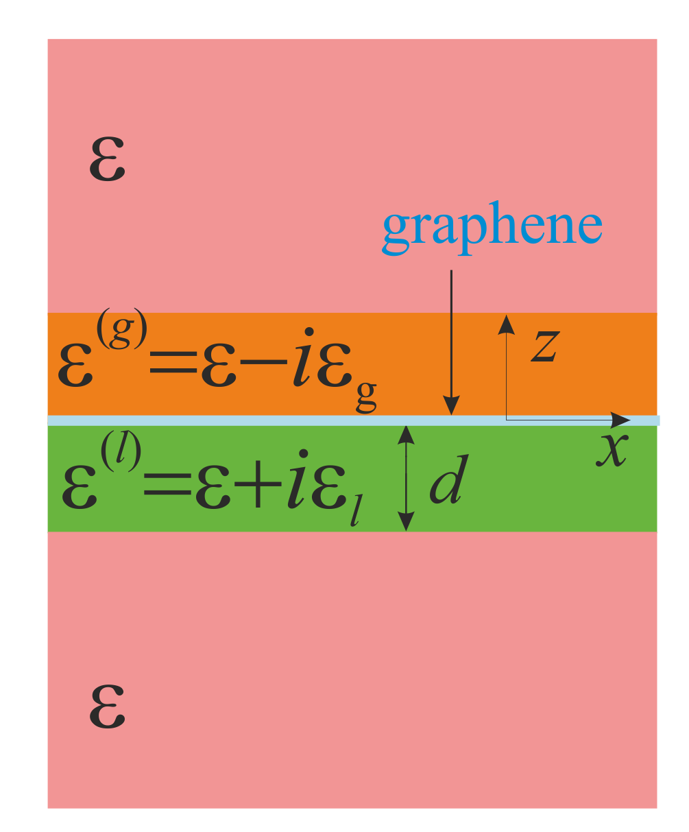
Figure 1: The graphene layer, embedded into the dielectric with spatially separated gain and losses.

We consider the graphene layer [see Fig. 1] cladded between the two dielectric media of equal thickness $d$, one of which is arranged at spatial domain $-d<z<0$ and is characterized by losses (dielectric constant $\varepsilon^{(l)}=\varepsilon+i\varepsilon_{l}$), while another one occupies spatial domain $0<z<d$ and is characterized by gain, $\varepsilon^{(g)}=\varepsilon-i\varepsilon_{g}$. The half-spaces outside the described domains are filled with the lossless dielectric with permittivity $\varepsilon$.

Since GSPPs are p-polarized waves, in this paper we restrict our consideration to the case of TM polarization, which is described by Maxwell equations

$$-\frac{\partial H_{y}}{\partial z}=-\frac{i\omega}{c}\varepsilon\left(z\right)E_{x}+\frac{4\pi}{c}\sigma\left(\omega\right)E_{x}\delta\left(z\right),$$ (1)

$$ik_{x}H_{y}=-\frac{i\omega}{c}\varepsilon\left(z\right)E_{z},$$ (2)

$$\frac{\partial E_{x}}{\partial z}-ik_{x}E_{z}=\frac{i\omega}{c}H_{y}.$$ (3)

Here we admitted that the electric field of the p-polarized wave $\mathbf{E}=\left(E_{x},0,E_{z}\right)$ possesses nonzero $x$- and $z$-components, while in its magnetic field only $y$-component is nonzero, i.e. $\mathbf{H}=\left(0,H_{y},0\right)$. Also in Maxwell equations (1)–(3) we take into account the uniformity of the structure in $y$-direction (i.e. $\partial/\partial y\equiv 0$), spatiotemporal dependence of the electromagnetic field $\sim\exp\left(ik_{x}x-i\omega t\right)$ [where $\omega$ is the cyclic frequency, $k_{x}$ is the in-plane component of the wavevector, and $c$ stands for the light velocity in vacuum] as well as the spatial dependence of the dielectric constant

$$\varepsilon\left(z\right)=\left\{\begin{array}[]{cc}\varepsilon,&\left|z\right|>d\\ \varepsilon^{(l)},&-d<z<0\\ \varepsilon^{(g)},&0<z<d.\end{array}\right.$$ (7)

At the same time, in Eqs. (1)–(3) Dirac delta expresses the two-dimensional character of graphene’s conductivity $\sigma\left(\omega\right)$, which can be expressed in Drude form as

$$\sigma\left(\omega\right)=\frac{e^{2}}{4\hbar}\frac{4E_{F}}{\pi\hbar\left(\gamma-i\omega\right)}.$$ (8)

Here $E_{F}$ is the Fermi energy and $\gamma$ is the disorder. In practice, graphene monolayer is characterized by the finite thickness $\approx 3\,$Å. But further in the paper the thickness of graphene is supposed to be much less than thicknesses of gainy and lossy dielectric layers, so the graphene is considered as two-dimensional conductor.

In the semiinfinite spatial domain $z<-d$, the solution of Maxwell equations (1)–(3) can be represented as

$$H_{y}^{\left(-\right)}\left(z\right)=H_{y}^{\left(-\right)}\left(-d\right)\exp\left[p\left(z+d\right)\right],$$ (9)

$$E_{x}^{\left(-\right)}\left(z\right)=\frac{cp}{i\omega\varepsilon}H_{y}^{\left(-\right)}\left(-d\right)\exp\left[p\left(z+d\right)\right],$$ (10)

$$E_{z}^{\left(-\right)}\left(z\right)=-\frac{ck_{x}}{\omega\varepsilon}H_{y}^{\left(-\right)}\left(-d\right)\exp\left[p\left(z+d\right)\right].$$ (11)

Here $H_{y}^{\left(-\right)}\left(-d\right)$ and $p=\left[k_{x}^{2}-\left(\omega/c\right)^{2}\varepsilon\right]^{1/2}$ are the value of magnetic field at $z=-d$ and its decaying factor, respectively. The electromagnetic wave, whose fields are described by Eqs. (9)–(11) can be either evanescent (when $k_{x}>\omega\sqrt{\varepsilon}/c$, and $p$ is purely real value, which sign is chosen to be positive in this case, $\mathrm{Re}\left[p\right]>0$), or propagating (when $k_{x}<\omega\sqrt{\varepsilon}/c$, and $p$ is purely imaginary with $\mathrm{Im}\left[p\right]<0$). Such condition for signs of the real and imaginary parts of $p$ along with the positiveness of the sign of the argument of the exponent $\exp\left[p\left(z+d\right)\right]$ describes the situation, where the evanescent wave decays in the direction towards $z\to-\infty$, while the propagating wave propagates in the negative direction of $z$-axis.

In other semiinfinite domain $z>d$ the solution of Maxwell equations (1)–(3) can be expressed in the form

$$H_{y}^{\left(+\right)}\left(z\right)=H_{y}^{\left(+\right)}\left(d\right)\exp\left[-p\left(z-d\right)\right],$$ (12)

$$E_{x}^{\left(+\right)}\left(z\right)=-\frac{cp}{i\omega\varepsilon}H_{y}^{\left(+\right)}\left(d\right)\exp\left[-p\left(z-d\right)\right],$$ (13)

$$E_{z}^{\left(+\right)}\left(z\right)=-\frac{ck_{x}}{\omega\varepsilon}H_{y}^{\left(+\right)}\left(d\right)\exp\left[-p\left(z-d\right)\right],$$ (14)

where $H_{y}^{\left(+\right)}\left(d\right)$ is value of the magnetic field at $z=d$. Owing to the negativeness of the sign of the exponent’s argument $\exp\left[-p\left(z-d\right)\right]$ the wave either decays towards $z\to\infty$, or propagates in the positive direction of the axis $z$.

In the dielectric with losses the solutions of Maxwell equation will have form

$$H_{y}^{\left(l\right)}\left(z\right) = H_{y}^{\left(l\right)}\left(-d\right)\cos\left[k_{z}^{(l)}\left(z+d\right)\right]$$

$$+\frac{i\omega\varepsilon^{(l)}}{ck_{z}^{(l)}}E_{x}^{\left(l\right)}\left(-d\right)\sin\left[k_{z}^{(l)}\left(z+d\right)\right],$$

$$E_{x}^{\left(l\right)}\left(z\right) = E_{x}^{\left(l\right)}\left(-d\right)\cos\left[k_{z}^{(l)}\left(z+d\right)\right]$$

$$-\frac{ck_{z}^{(l)}}{i\omega\varepsilon^{(l)}}H_{y}^{\left(l\right)}\left(-d\right)\sin\left[k_{z}^{(l)}\left(z+d\right)\right],$$

$$E_{z}^{\left(l\right)}\left(z\right) = -\frac{ck_{x}}{\omega\varepsilon^{(l)}}\left\{H_{y}^{\left(l\right)}\left(-d\right)\cos\left[k_{z}^{(l)}\left(z+d\right)\right]\right.$$

$$\left.+\frac{i\omega\varepsilon^{(l)}}{ck_{z}^{(l)}}E_{x}^{\left(l\right)}\left(-d\right)\sin\left[k_{z}^{(l)}\left(z+d\right)\right]\right\},$$

where $k_{z}^{(l)}=\left[\left(\omega/c\right)^{2}\varepsilon^{(l)}-k_{x}^{2}\right]^{1/2}$ , $E_{x}^{\left(l\right)}\left(-d\right)$ and $H_{y}^{\left(l\right)}\left(-d\right)$ being the values of the tangential components of the electric and magnetic fields at the boundary of the medium with losses $z=-d$. In the similar manner the electromagnetic field in the medium with gain can be represented as

$$H_{y}^{\left(g\right)}\left(z\right) = H_{y}^{\left(g\right)}\left(0\right)\cos\left[k_{z}^{(g)}z\right]$$

$$+\frac{i\omega\varepsilon^{(g)}}{ck_{z}^{(g)}}E_{x}^{\left(g\right)}\left(0\right)\sin\left[k_{z}^{(g)}z\right],$$

$$E_{x}^{\left(g\right)}\left(z\right) = E_{x}^{\left(g\right)}\left(0\right)\cos\left[k_{z}^{(g)}z\right]$$

$$-\frac{ck_{z}^{(g)}}{i\omega\varepsilon^{(g)}}H_{y}^{\left(g\right)}\left(0\right)\sin\left[k_{z}^{(g)}z\right],$$

$$E_{z}^{\left(g\right)}\left(z\right) = -\frac{ck_{x}}{\omega\varepsilon^{(g)}}\left\{H_{y}^{\left(g\right)}\left(0\right)\cos\left[k_{z}^{(g)}z\right]\right.$$

$$\left.+\frac{i\omega\varepsilon^{(g)}}{ck_{z}^{(g)}}E_{x}^{\left(g\right)}\left(0\right)\sin\left[k_{z}^{(g)}z\right]\right\},$$

Here $k_{z}^{(g)}=\left[\left(\omega/c\right)^{2}\varepsilon^{(g)}-k_{x}^{2}\right]^{1/2}$, while $E_{x}^{\left(g\right)}\left(0\right)$ and $H_{y}^{\left(g\right)}\left(0\right)$ stand for the values of the tangential components of the electric and magnetic fields, correspondingly at the boundary of the medium with gain $z=0$.

Boundary conditions for the tangential components of the electric and magnetic fields can be obtained directly from Maxwell equations (1)–(3). Thus, integrating of (3) over the infinitesimal interval $[d-0,d+0]$ gives the boundary condition

$$E_{x}^{(+)}\left(d\right)=E_{x}^{(g)}\left(d\right),$$ (21)

which couples the tangential component of the electric field across the boundary between the gainy and lossless dielectrics. In the similar manner, integration of (3) over the intervals $[-0,+0]$ and $[-d-0,-d+0]$ results in boundary conditions

$$E_{x}^{(l)}\left(0\right)=E_{x}^{(g)}\left(0\right),$$ (22)

$$E_{x}^{(l)}\left(-d\right)=E_{x}^{(-)}\left(-d\right)$$ (23)

for the electric field tangential component across the graphene layer and at the boundary between dissipative and lossless dielectrics, respectively.

Boundary conditions for the tangential component of the magnetic field can be obtained from integration of Eq. (1) over the same infinitesimal intervals as in the previous case. The final expressions can be represented in the form

$$H_{y}^{(+)}\left(d\right)=H_{y}^{(g)}\left(d\right),$$ (24)

$$H_{y}^{(g)}\left(0\right)=H_{y}^{(l)}\left(0\right)-\frac{4\pi}{c}\sigma\left(\omega\right)E_{x}^{(l)}\left(0\right),$$ (25)

$$H_{y}^{(l)}\left(-d\right)=H_{y}^{(-)}\left(-d\right).$$ (26)

In other words, at boundaries $z=\pm d$ magnetic field is continuous across the interface, while at the interface $z=0$ the magnetic field is discontunuous across the graphene due to presence of currents in it.

Substitution of Eqs. (9), (10), (2), and (2) into Eqs. (23) and (26) results into

$$H_{y}^{\left(l\right)}\left(-d\right)=H_{y}^{\left(-\right)}\left(-d\right),$$ (27)

$$E_{x}^{\left(l\right)}\left(-d\right)=\frac{cp}{i\omega\varepsilon}H_{y}^{\left(-\right)}\left(-d\right).$$ (28)

In similar manner, substitution of Eqs. (12), (13), (2), and (2) into boundary conditions (21) and (24) gives

$$H_{y}^{\left(+\right)}\left(d\right)=H_{y}^{\left(g\right)}\left(d\right),$$ (29)

$$-\frac{cp}{i\omega\varepsilon}H_{y}^{\left(+\right)}\left(d\right)=E_{x}^{\left(g\right)}\left(d\right).$$ (30)

In the matrix form the above equations can be represented as

$$\hat{F}^{(l)}\left(-d\right)=\hat{\mathcal{S}}^{(-)}H_{y}^{(-)}\left(-d\right),$$ (31)

$$\hat{F}^{(g)}\left(d\right)=\hat{\mathcal{S}}^{(+)}H_{y}^{(+)}\left(d\right),$$ (32)

where $\hat{\mathcal{S}}^{(\pm)}$ and $\hat{F}^{(f)}\left(z\right)$ are 2$\times$1 matrices

$$\hat{\mathcal{S}}^{(\pm)}=\left(\begin{array}[]{c}1\\ \mp\frac{cp}{i\omega\varepsilon}\end{array}\right),$$ (35)

$$\hat{F}^{(f)}\left(z\right)=\left(\begin{array}[]{c}H_{y}^{\left(f\right)}\left(z\right)\\ E_{x}^{\left(f\right)}\left(z\right)\end{array}\right),$$ (38)

and index $f=g,l$. Along with this, representation of boundary conditions (22) and (25) in the matrix form results in

$$\hat{F}^{(g)}\left(0\right)=\hat{\mathcal{G}}\hat{F}^{(l)}\left(0\right),$$ (39)

where $\hat{\mathcal{G}}$ is the 2$\times$2 matrix

$$\hat{\mathcal{G}}=\left(\begin{array}[]{cc}1&-\frac{4\pi}{c}\sigma\left(\omega\right)\\ 0&1\end{array}\right).$$ (42)

Along with this, from Eqs. (2) and (2) it is possible to link the fields at $z=-d$ and $z=0$ as

$$\hat{F}^{(l)}\left(0\right)=\hat{\mathcal{T}}^{(l)}\hat{F}^{(l)}\left(-d\right).$$ (43)

In similar manner from Eqs. (2) and (2) one can obtain

$$\hat{F}^{(g)}\left(d\right)=\hat{\mathcal{T}}^{(g)}\hat{F}^{(g)}\left(0\right).$$ (44)

In above equations the transfer-matrices

$$\hat{\mathcal{T}}^{(f)}=\left(\begin{array}[]{cc}\cos\left[k_{z}^{(f)}d\right]&\frac{i\omega\varepsilon^{(f)}}{ck_{z}^{(f)}}\sin\left[k_{z}^{(f)}d\right]\\ -\frac{ck_{z}^{(f)}}{i\omega\varepsilon^{(f)}}\sin\left[k_{z}^{(f)}d\right]&\cos\left[k_{z}^{(f)}d\right]\end{array}\right).$$ (47)

Applying consequently the boundary conditions (31), (39), and (32) [along with Eqs. (43) and (44)], we obtain

$$\hat{\mathcal{S}}^{(+)}H_{y}^{(+)}\left(d\right)=\hat{\mathcal{T}}^{(g)}\hat{\mathcal{G}}\hat{\mathcal{T}}^{(l)}\hat{\mathcal{S}}^{(-)}H_{y}^{(-)}\left(-d\right).$$ (48)

This equation, being multiplied by row matrix

$$\left\{\hat{\mathcal{S}}^{(-)}\right\}^{-1}=\frac{1}{2}\left(\begin{array}[]{cc}1&\frac{i\omega\varepsilon}{cp}\end{array}\right),$$ (50)

after taking into account orthogonality of matrices

$$\left\{\hat{\mathcal{S}}^{(-)}\right\}^{-1}\hat{\mathcal{S}}^{(+)}=0$$ (51)

results in the dispersion relation of the waves in the graphene-based structure

$$\left\{\hat{\mathcal{S}}^{(-)}\right\}^{-1}\hat{\mathcal{T}}^{(g)}\hat{\mathcal{G}}\hat{\mathcal{T}}^{(l)}\hat{\mathcal{S}}^{(-)}=0,$$ (52)

which can be written in the explicit form as

$$\frac{\varepsilon^{(g)}}{k_{z}^{(g)}}\Phi^{(g)}+\frac{\varepsilon^{(l)}}{k_{z}^{(l)}}\Phi^{(l)}+\frac{4\pi}{i\omega}\sigma\left(\omega\right)=0,$$ (53)

where

$$\Phi^{(f)}=\frac{\cos\left[k_{z}^{(f)}d\right]+\frac{\varepsilon^{(f)}p}{\varepsilon k_{z}^{(f)}}\sin\left[k_{z}^{(f)}d\right]}{\sin\left[k_{z}^{(f)}d\right]-\frac{\varepsilon^{(f)}p}{\varepsilon k_{z}^{(f)}}\cos\left[k_{z}^{(f)}d\right]}.$$ (54)

3 $\mathcal{PT}$-symmetric surface plasmon-polaritons

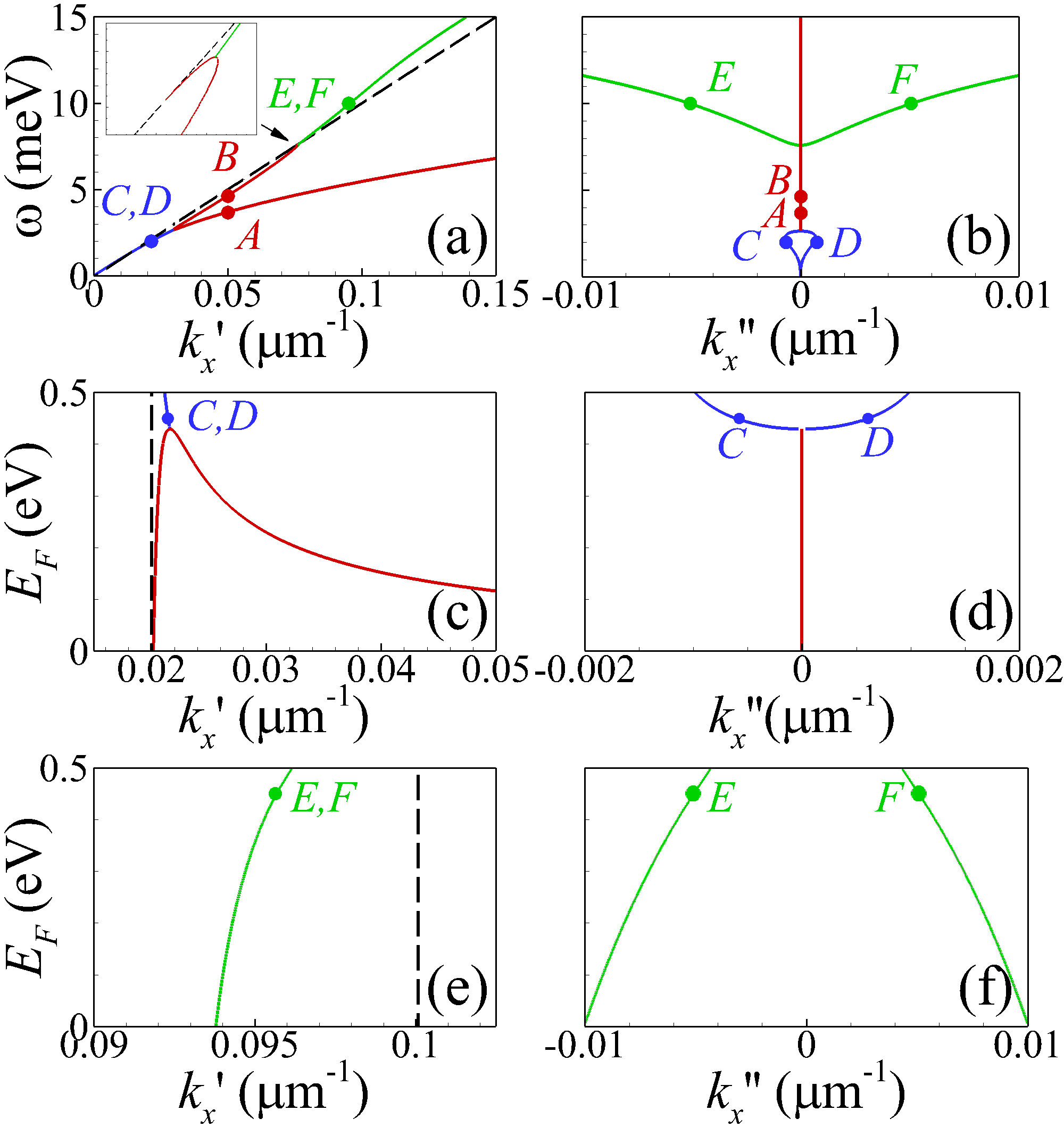
Figure 2: (a,b) Dispersion relation of the graphene SPPs in the $\mathcal{PT}$-symmetric surrounding for fixed Fermi energy $E_{F}=0.45\,$eV – panels (a) and (b) present the frequency dependence of the real $k_{x}^{\prime}\left(\omega\right)$ and imaginary $k_{x}^{\prime\prime}\left(\omega\right)$ parts of the wavevector, correspondingly; (c–f) Dependence of real [panels (c) and (e)] and imaginary [panels (d) and (f)] parts of wavevector ($k_{x}^{\prime}$ and $k_{x}^{\prime\prime},$respectively) upon the Fermi energy $E_{F}$ for two frequencies $\omega=2\,$meV [panels (c) and (d)] and $\omega=10\,$meV [panels (e) and (f)]. In all panels dispersion curves of graphene SPPs with unbroken $\mathcal{PT}$-symmetry are depicted by solid red lines, while those with broken PT-symmetry are depicted by solid blue and green lines. Dashed lines in panels (a), (c), and (e) stand for the light line $k_{x}^{\prime}=\omega\sqrt{\varepsilon}/c$. Other parameters of the structure are: $\varepsilon=3.9$, $\varepsilon^{(g)}=\varepsilon^{(l)}=1.9$, $d=40\,\mu$m, $\gamma=0$.

In the particular situation, when the graphene is considered to be lossless ($\gamma=0$) and the gain and losses in surrounding media are prefectly balanced ($\varepsilon_{g}=\varepsilon_{l}$), the dielectric function (7) is characterized by the property $\varepsilon\left(z\right)=\varepsilon^{*}\left(-z\right)$. In other words, graphene-based structure possesses the $\mathcal{PT}$-symmetry, whose distinctive properties are revealed in the dispersion relation of GSPPs [see Figs. (2)(a) and (2)(b)]. It should be noted that Figs. (2)(a) and (2)(b) represent the solution of the dispersion relation (53), when the frequency $\omega$ is supposed to be purely real value, while the in-plane wavevector $k_{x}=k_{x}^{\prime}+ik_{x}^{\prime\prime}$ is supposed to be complex value, whose imaginary part characterizes the degree of exponential decaying (when $k_{x}^{\prime\prime}>0$) or growing (when $k_{x}^{\prime\prime}<0$) of wave’s amplitude per unit length during the propagation along $x$-axis.

In the conservative system (without gain/losses) the dispersion relation of GSPP possesses one branch [for details see, e.g. Ref. [51]], which exists in the whole range of the wavevectors and frequencies. The situation changes drastically in the case of $\mathcal{PT}$-symmetry. Thus, in the lossless graphene in $\mathcal{PT}$-symmetric dielectric surrounding there are two modes of GSPPs with unbroken $\mathcal{PT}$-symmetry – low-frequency mode [red solid line A in Fig. 2(a)] and high-frequency one [red solid line B in Fig. 2(a)]. Unbroken $\mathcal{PT}$-symmetry are characterized by zero imaginary part of these modes’ wavevectors [$k_{x}^{\prime\prime}\equiv 0$, see Fig. 2(b)]. In other words, these modes propagate along the graphene layer without damping or growth. At the exceptional point, located at $\omega\approx 2.025\,$meV and $k_{x}^{\prime}\approx 0.0218\,\mu\mathrm{m}^{-1}$, low- and high-frequency modes merge together, and GSPPs with frequencies below this exceptional point are characterized by broken $\mathcal{PT}$-symmetry. Here spectrum contains two modes [solid blue lines C and D in Figs. 2(a) and 2(b)] with complex wavevectors $k_{x}$ such that for given frequency wavevector of one mode is complex conjugate of the other mode’s wavevector. As a result, one GSPP mode [mode C in Figs. 2(a) and 2(b)] is exponentially growing during its propagation along the graphene, and another mode is exponentially decaying [mode D in Figs. 2(a) and 2(b)]. At the same time high-frequency GSPP mode with unbroken $\mathcal{PT}$-symmetry [line B in Figs. 2(a) and 2(b)] at another exceptional point [$\omega\approx 7.58\thinspace$eV and $k_{x}\approx 0.0762\thinspace\mu\mathrm{m}^{-1}$] folds towards light line $\omega=ck_{x}/\sqrt{\varepsilon}$ and has end-point of the spectrum lying on this light line [which is depicted by dashed black line in Fig. 2(a)]. Along with this, at that exceptional point [see inset in Fig. 2(a)] GSPP mode with unbroken $\mathcal{PT}$-symmetry transforms into pair of modes with broken $\mathcal{PT}$-symmetry [green solid lines E and F in Figs. 2(a) and 2(b)], which degree of growth/decay (imaginary part of the wavevector $k_{x}^{\prime\prime}$) increases monotonically with an increase of frequency.

One of the advantages of using graphene in plasmonics is the possibility to tune dynamically graphene’s Fermi energy (and, consequently, the dispersion properties of GSPPs) in time simply by changing the gate voltage applied to graphene. Respective dependence between the Fermi energy and bias voltage $V_{b}$, applied to graphene, can be expressed as $E_{F}\sim\left(V_{b}\right)^{1/2}$ [see, e.g., Refs.[52, 27, 53]]. In $\mathcal{PT}$-symmetric graphene-based structures it opens another possibility – to switch dynamically between the unbroken and broken $\mathcal{PT}$-symmetries. An example of such situation is demonstrated in Figs. 2(c) and 2(d), where for the fixed frequency $\omega=2\thinspace$meV graphene’s Fermi energies above and below $E_{F}\approx 0.429\,$eV give rise to the broken and unbroken $\mathcal{PT}$-symmetries, respectively. Notice, that upper mode E and F [see Figs. 2(e) and 2(f)] for chosen fixed frequency $\omega=10\,$meV, and dielectric constant’s imaginary part $\varepsilon_{g}=\varepsilon_{l}=1.9$ exhibits broken $\mathcal{PT}$-symmetry in all range of nowadays exterimentally attainable [28] graphene’s Fermi energies $E_{F}\lesssim 0.5\,$eV. Such a mode can exist even when graphene is absent (case $E_{F}=0$) – respective modes were investigated in Ref. [54].

The physical origins of the reported phenomena can be understood from spatial distributions of the electromagnetic field, which are shown in Fig. 3. In the case of unbroken $\mathcal{PT}$-symmetry [see Figs. 3(a) and 3(b) for low- and high-frequency modes A and B, correspondingly] in-plane component of the electric field possesses reflective symmetry (real part, depicted by solid red lines) or antisymmetry (imaginary part, depicted by dashed blue lines) with respect to the graphene layer, which is located at the boundary between the gainy and lossy medium at $z=0$. In other words, their field distribution obey the $\mathcal{PT}$-symmetric relation $E_{x}^{(A)}\left(z\right)=\left\{E_{x}^{(A)}\left(-z\right)\right\}^{*}$, $E_{x}^{(B)}\left(z\right)=\left\{E_{x}^{(B)}\left(-z\right)\right\}^{*}$. Equality of the field amplitudes in gainy and lossy media originates a perfect balance between gain and losses of energy during the propagation, which in its turn lead to the propagation of GSPPs with constant amplitude. For broken $\mathcal{PT}$-symmetry [see Figs. 3(c)–3(f) for modes C–F, respectively], the spatial profiles $E_{x}\left(z\right)$ are asymetric. Meanwhile, for modes C and E most of the field is concentrated in the medium with gain, while for modes D and F most of the field is concentrated in lossy medium, which determines respective growing of decaying of energy during mode propagation along the graphene. At the same time, modes with broken $\mathcal{PT}$-symmetry possess the mutual symmetry $E_{x}^{(C)}\left(z\right)=\left\{E_{x}^{(D)}\left(-z\right)\right\}^{*}$, $E_{x}^{(E)}\left(z\right)=\left\{E_{x}^{(F)}\left(-z\right)\right\}^{*}$, which determines the equality of absolute values of the imaginary parts of their wavevectors.

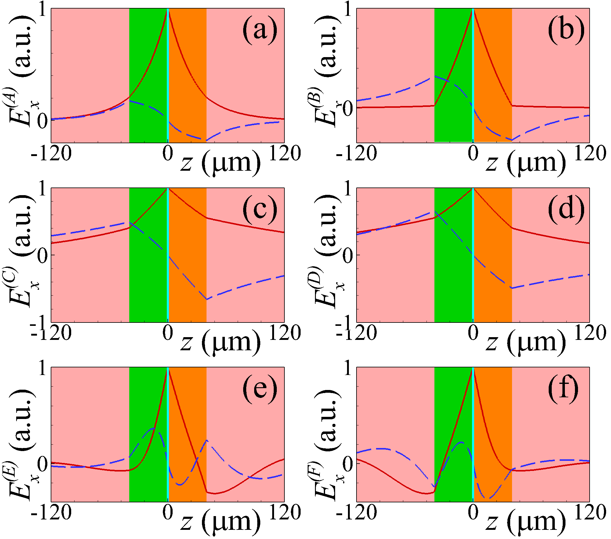
Figure 3: Spatial profiles of the electric field in-plane component $E_{x}\left(z\right)$ for frequency $\omega=3.684\,$meV and wavevector $k_{x}=0.05\,\mu\mathrm{m}^{-1}$ [panel (a)]; $\omega=4.642\,$meV, $k_{x}=0.05\,\mu\mathrm{m}^{-1}$ [panel (b)]; $\omega=2\,$meV, $k_{x}=\left(0.0215-i0.0006\right)\,\mu\mathrm{m}^{-1}$ [panel (c)]; $\omega=2\,$meV, $k_{x}=\left(0.0215+i0.0006\right)\,\mu\mathrm{m}^{-1}$ [panel (d)]; $\omega=10\,$meV, $k_{x}=\left(0.0957-i0.0051\right)\,\mu\mathrm{m}^{-1}$ [panel (e)]; $\omega=10\,$meV, $k_{x}=\left(0.0957+i0.0051\right)\,\mu\mathrm{m}^{-1}$ [panel (f)]. Other parameters are the same as those in Fig. (2)(a). The frequencies $\omega$ and wavevectors $k_{x}$ of the profles in panels (a)–(f), are depicted in Fig. (2) by points A–F, respectively (which are depicted as superindexes in y-axis titles). Real and imaginary parts of the electric field are depicted by solid red and dashed blue lines, respectively.

4 Graphene surface plasmon-polaritons in dielectric medium with unbalanced gain and losses

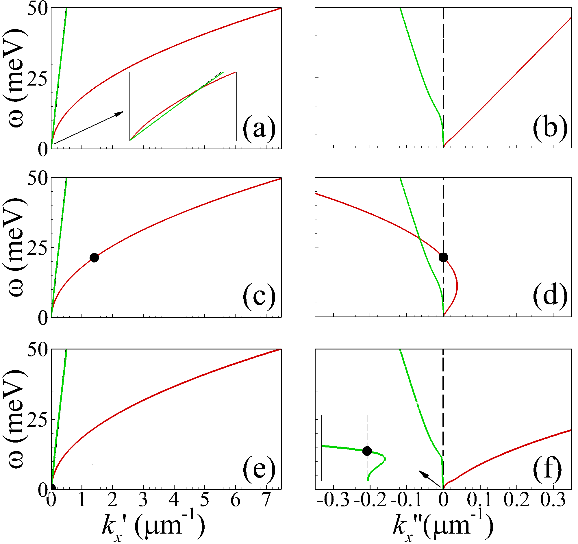
Figure 4: Dispersion relation $k_{x}\left(\omega\right)$ of surface plasmon-polaritons, propagating in lossy graphene monolayer with Fermi energy $E_{F}=0.45\thinspace$eV and disorder $\gamma=2.5\thinspace$meV, arranged in the dielectric surrounding with gain/losses $\varepsilon^{(g)}=\varepsilon^{(l)}=1.9$ [panels (a) and (b)], $\varepsilon^{(g)}=1.9$, $\varepsilon^{(l)}=1$ [panels (c) and (d)], or $\varepsilon^{(g)}=1.9$, $\varepsilon^{(l)}=3$ [panels (e) and (f)]. Left column [panels (a), (c), and (e)] corresponds to the real part of the wavevector $k_{x}^{\prime}$, while the right one [panels (b), (d), and (f)] – to the imaginary part $k_{x}^{\prime\prime}$. Other parameters of the structure are the same as those in Fig. 2. Black dots in panels (c) and (d) depict the frequency and wavevector of GSPP’s spectral singularity.

Now a natural question appears: how the dispersion properties will change, if graphene monolayer is not lossless? To answer this question we represent in Figs. 4(a) and 4(b) the disperion curves of the GSPPs in the case where gain and losses in surrounding dielectric media are mutually balanced, but small losses are present in graphene [$\gamma\neq 0$ in Eq. (8)]. As evident, losses in graphene results in the situation, where the GSPP spectrum ceases to be real. In more detail, the low-frequency mode (solid red lines) is decaying (with positive $k_{x}^{\prime\prime}>0$) in all range of the frequencies and wavevectors, while high-frequency one (green solid lines) is growing (with negative $k_{x}^{\prime\prime}<0$). Nevertheless, if in the dielectric surrounding gain prevails over losses [see Figs. 4(c) and 4(d)], then the low-frequency mode becomes growing at frequencies above some threshold frequency [$\omega\approx 21.38\,$meV for the parameters of Figs. 4(c) and 4(d)], and remains decaying at frequencies below this threshold. This threshold frequency [called spectral singularity and depicted in Figs 4(c) and 4(d) by black dots] plays an important role – it is the only frequency in all frequency domain, where GSPP spectrum is characterized by purely real wavevector [$k_{x}\approx 1.41\,\mu$m^-1 for the parameters of Figs. 4(c) and 4(d)]. In other words, GSPP with frequency, corresponding to spectral singularity, propagates along graphene without growth or damping, owing to its real wavevector. At the same time, when in layered structure losses are higher than gain [Figs. 4(e) and 4(f)], the high-frequency mode contains the spectral singularity at frequency $\omega\approx 0.44\,$meV.

In connection with this a next question arises: is it possible to tune the position of spectral singularity by varying the Fermi energy? The answer to this question follows directly from Figs. 5(a) and 5(b). Thus, for given Fermi energy $E_{F}$ (horizontal axis) it is possible to find such frequency $\omega$ (left vertical axis) of spectral singularity, at which GSPP spectrum will be characterized by purely real wavevector $k_{x}$ (right vertical axis). Even more, from comparison of Figs. 5(a) and 5(b) it follows, that lowering of losses [Fig. 5(b)] in dielectric leads to the red-shift of the spectral singularity. At the same time for fixed Fermi energy losses in graphene exert strong influence on the position of spectral singularity [see Fig. 5(c)]. Thus, lowering the graphene’s disorder $\gamma$ leads to decrease of the respective frequency and wavevector of spectral singularity.

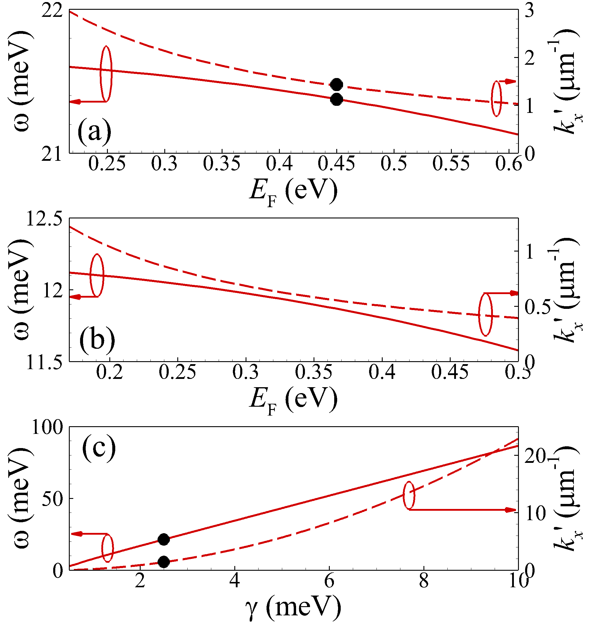
Figure 5: Dependence of GSPP spectral singularity’s frequency $\omega$ (solid lines, left axis) and wavevector $k_{x}^{\prime}$ (dashed lines, right axis) upon graphene’s Fermi energy [panels (a) and (b)] or upon the disorder in graphene $\gamma$ [panel (c)]. The parameters of the structure are: $\gamma=2.5\thinspace$meV [panels (a) and (b)], $E_{F}=0.45\,$eV [panel (c)], $d=40\,\mu$m, $\varepsilon=3.9$, $\varepsilon^{(g)}=1.9$, $\varepsilon^{(l)}=1.0$ [panel (a) and (c)], $\varepsilon^{(l)}=0.3$ [panel (b)]. In panels (a) and (c) black dots depict the same parameters of spectral singularity as those in Figs. 4(c) and 4(d).

5 Conclusions

To conclude, we considered spectrum of GSPPs in the structure, where graphene monolayer is cladded between two dielectric slabs of finite thickness – one slab with gain and another with losses. We demonstrated that in the case of $\mathcal{PT}$-symmetric dielectric surrounding the spectrum consists of two modes, which coalescs at exceptional point. At the frequency ranges below and above the exceptional point the $\mathcal{PT}$-symmetry is broken and unbroken, respectively. The position of the exceptional point is sensitive to the Fermi energy of graphene. Last fact opens the possibility to switch dynamically between the broken and unbroken $\mathcal{PT}$-symmetry by means of the electrostatic gating, i.e. by changing the gate voltage, applied to graphene. When gain and losses in dielectric slabs are not mutually balanced and graphene is lossy, the GSPP spectrum in such system is characterized by the presence of spectral singularity – at certain particular frequency the GSPP propagation is lossless, i.e. respective GSPP is characterized by infinite mean free path and can travel along graphene monolayer with constant amplitude – without decaying ou growth. In its turn the electrostatic gating of graphene (varying the Fermi energy) allows to change the frequency of spectral singularity.

References

- Bender and Boettcher [1998] Carl M. Bender and Stefan Boettcher. Real Spectra in Non-Hermitian Hamiltonians Having PT Symmetry. Physical Review Letters, 80(24):5243–5246, jun 1998. ISSN 0031-9007. doi:10.1103/PhysRevLett.80.5243. URL http://link.aps.org/doi/10.1103/PhysRevLett.80.5243.
- Bender et al. [2013] Carl M. Bender, Bjorn K. Berntson, David Parker, and E. Samuel. Observation of PT phase transition in a simple mechanical system. Am. J. Phys, 81(3):173–179, mar 2013. ISSN 0002-9505. doi:10.1119/1.4789549. URL http://aapt.scitation.org/doi/10.1119/1.4789549.
- Fleury et al. [2015] Romain Fleury, Dimitrios Sounas, and Andrea Alù. An invisible acoustic sensor based on parity-time symmetry. Nature Communications, 6:5905, jan 2015. ISSN 2041-1723. doi:10.1038/ncomms6905. URL http://www.nature.com/doifinder/10.1038/ncomms6905.
- Schindler et al. [2011] Joseph Schindler, Ang Li, Mei C. Zheng, F. M. Ellis, and Tsampikos Kottos. Experimental study of active LRC circuits with PT symmetries. Phys. Rev. A, 84(4):040101, oct 2011. ISSN 1050-2947. doi:10.1103/PhysRevA.84.040101. URL http://link.aps.org/doi/10.1103/PhysRevA.84.040101.
- Guo et al. [2009] A. Guo, G. J. Salamo, D. Duchesne, R. Morandotti, M. Volatier-Ravat, V. Aimez, G. A. Siviloglou, and D. N. Christodoulides. Observation of PT-Symmetry Breaking in Complex Optical Potentials. Physical Review Letters, 103(9):093902, aug 2009. ISSN 0031-9007. doi:10.1103/PhysRevLett.103.093902. URL http://link.aps.org/doi/10.1103/PhysRevLett.103.093902.
- Rüter et al. [2010] Christian E. Rüter, Konstantinos G. Makris, Ramy El-Ganainy, Demetrios N. Christodoulides, Mordechai Segev, and Detlef Kip. Observation of parity-time symmetry in optics. Nature Physics, 6(3):192–195, jan 2010. ISSN 1745-2473. doi:10.1038/nphys1515. URL http://www.nature.com/doifinder/10.1038/nphys1515.
- Regensburger et al. [2012] Alois Regensburger, Christoph Bersch, Mohammad-Ali Miri, Georgy Onishchukov, Demetrios N. Christodoulides, and Ulf Peschel. Parity-time synthetic photonic lattices. Nature, 488(7410):167–171, aug 2012. ISSN 0028-0836. doi:10.1038/nature11298. URL http://www.nature.com/doifinder/10.1038/nature11298.
- Peng et al. [2014] Bo Peng, Şahin Kaya Özdemir, Fuchuan Lei, Faraz Monifi, Mariagiovanna Gianfreda, Gui Lu Long, Shanhui Fan, Franco Nori, Carl M. Bender, and Lan Yang. Parity-time-symmetric whispering-gallery microcavities. Nature Physics, 10(5):394–398, apr 2014. ISSN 1745-2473. doi:10.1038/nphys2927. URL http://www.nature.com/doifinder/10.1038/nphys2927.
- Fleury et al. [2014] Romain Fleury, Dimitrios L. Sounas, and Andrea Alù. Negative Refraction and Planar Focusing Based on Parity-Time Symmetric Metasurfaces. Physical Review Letters, 113(2):023903, jul 2014. ISSN 0031-9007. doi:10.1103/PhysRevLett.113.023903. URL http://link.aps.org/doi/10.1103/PhysRevLett.113.023903.
- Valagiannopoulos et al. [2016] C A Valagiannopoulos, F Monticone, and A Alù. PT-symmetric planar devices for field transformation and imaging. Journal of Optics, 18(4):044028, apr 2016. ISSN 2040-8978. doi:10.1088/2040-8978/18/4/044028. URL http://stacks.iop.org/2040-8986/18/i=4/a=044028?key=crossref.feb59d6efc0f37cec2e475ecc5f4d263.
- Monticone et al. [2016] Francesco Monticone, Constantinos A. Valagiannopoulos, and Andrea Alù. Parity-Time Symmetric Nonlocal Metasurfaces: All-Angle Negative Refraction and Volumetric Imaging. Physical Review X, 6(4):041018, oct 2016. ISSN 2160-3308. doi:10.1103/PhysRevX.6.041018. URL https://link.aps.org/doi/10.1103/PhysRevX.6.041018.
- Longhi [2010] Stefano Longhi. PT -symmetric laser absorber. Physical Review A, 82(3):031801, sep 2010. ISSN 1050-2947. doi:10.1103/PhysRevA.82.031801. URL http://journals.aps.org/pra/abstract/10.1103/PhysRevA.82.031801.
- Sun et al. [2014] Yong Sun, Wei Tan, Hong-qiang Li, Jensen Li, and Hong Chen. Experimental Demonstration of a Coherent Perfect Absorber with PT Phase Transition. Physical Review Letters, 112(14):143903, apr 2014. ISSN 0031-9007. doi:10.1103/PhysRevLett.112.143903. URL https://link.aps.org/doi/10.1103/PhysRevLett.112.143903.
- Chong et al. [2011] Y D Chong, Li Ge, and A Douglas Stone. PT-Symmetry Breaking and Laser-Absorber Modes in Optical Scattering Systems. Phys. Rev. Lett., 106(9):093902, mar 2011. ISSN 0031-9007. doi:10.1103/PhysRevLett.106.093902. URL http://journals.aps.org/prl/abstract/10.1103/PhysRevLett.106.093902.
- Mostafazadeh [2013] Ali Mostafazadeh. Invisibility and PT symmetry. Physical Review A, 87(1):012103, 2013. ISSN 10502947. doi:10.1103/PhysRevA.87.012103.
- Lin et al. [2011] Zin Lin, Hamidreza Ramezani, Toni Eichelkraut, Tsampikos Kottos, Hui Cao, and Demetrios N. Christodoulides. Unidirectional Invisibility Induced by PT-Symmetric Periodic Structures. Physical Review Letters, 106(21):213901, may 2011. ISSN 0031-9007. doi:10.1103/PhysRevLett.106.213901. URL https://link.aps.org/doi/10.1103/PhysRevLett.106.213901.
- Ge et al. [2012] Li Ge, Y. D. Chong, and A. D. Stone. Conservation relations and anisotropic transmission resonances in one-dimensional PT-symmetric photonic heterostructures. Physical Review A, 85(2):023802, feb 2012. ISSN 1050-2947. doi:10.1103/PhysRevA.85.023802. URL http://link.aps.org/doi/10.1103/PhysRevA.85.023802.
- Alaeian and Dionne [2014a] Hadiseh Alaeian and Jennifer A Dionne. Parity-time-symmetric plasmonic metamaterials. Physical Review A, 89(3):033829, mar 2014a. ISSN 1050-2947. doi:10.1103/PhysRevA.89.033829. URL http://arxiv.org/abs/1306.0059http://link.aps.org/doi/10.1103/PhysRevA.89.033829.
- Barton et al. [2018] D. Barton, M. Lawrence, H. Alaeian, B. Baum, and J. Dionne. Parity-Time Symmetric Plasmonics, pages 301–349. Springer Singapore, Singapore, 2018. ISBN 978-981-13-1247-2. doi:10.1007/978-981-13-1247-2_12. URL https://doi.org/10.1007/978-981-13-1247-2_12.
- Yang and Lei Mei [2015] Fan Yang and Zhong Lei Mei. Guiding SPPs with PT-symmetry. Scientific Reports, 5(1):14981, dec 2015. ISSN 2045-2322. doi:10.1038/srep14981. URL http://dx.doi.org/10.1038/srep14981http://www.nature.com/articles/srep14981.
- Benisty et al. [2011] Henri Benisty, Aloyse Degiron, Anatole Lupu, André De Lustrac, Sébastien Chénais, Sébastien Forget, Mondher Besbes, Grégory Barbillon, Aurélien Bruyant, Sylvain Blaize, and Gilles Lérondel. Implementation of PT symmetric devices using plasmonics: principle and applications. Optics Express, 19(19):18004, sep 2011. ISSN 1094-4087. doi:10.1364/OE.19.018004. URL http://www.ncbi.nlm.nih.gov/pubmed/21935166https://www.osapublishing.org/oe/abstract.cfm?uri=oe-19-19-18004.
- Baum et al. [2015] Brian Baum, Hadiseh Alaeian, and Jennifer Dionne. A parity-time symmetric coherent plasmonic absorber-amplifier. Journal of Applied Physics, 117(6):063106, feb 2015. ISSN 0021-8979. doi:10.1063/1.4907871. URL http://aip.scitation.org/doi/10.1063/1.4907871.
- Alaeian and Dionne [2014b] Hadiseh Alaeian and Jennifer a. Dionne. Non-Hermitian nanophotonic and plasmonic waveguides. Physical Review B, 89(7):075136, feb 2014b. ISSN 1098-0121. doi:10.1103/PhysRevB.89.075136. URL https://link.aps.org/doi/10.1103/PhysRevB.89.075136.
- Wang et al. [2017] Wei Wang, Lu-Qi Wang, Rui-Dong Xue, Hao-Ling Chen, Rui-Peng Guo, Yongmin Liu, and Jing Chen. Unidirectional Excitation of Radiative-Loss-Free Surface Plasmon Polaritons in PT-Symmetric Systems. Physical Review Letters, 119(7):077401, aug 2017. ISSN 0031-9007. doi:10.1103/PhysRevLett.119.077401. URL https://link.aps.org/doi/10.1103/PhysRevLett.119.077401.
- Nikitin et al. [2011] A Yu Nikitin, F Guinea, Francisco J. García-Vidal, and Luis Martín-Moreno. Fields radiated by a nanoemitter in a graphene sheet. Physical Review B, 84(19):195446, nov 2011. ISSN 1098-0121. doi:10.1103/PhysRevB.84.195446. URL http://arxiv.org/abs/1104.3558http://link.aps.org/doi/10.1103/PhysRevB.84.195446.
- Koppens et al. [2011] Frank H. L. Koppens, Darrick E Chang, and F. Javier García de Abajo. Graphene Plasmonics: A Platform for Strong Light-Matter Interactions. Nano Letters, 11(8):3370–3377, aug 2011. ISSN 1530-6984. doi:10.1021/nl201771h. URL http://pubs.acs.org/doi/abs/10.1021/nl201771h.
- Li et al. [2008] Z Q Li, E A Henriksen, Z Jiang, Zhao Hao, Michael C Martin, P Kim, H L Stormer, and Dimitri N. Basov. Dirac charge dynamics in graphene by infrared spectroscopy. Nature Physics, 4(7):532–535, jun 2008. ISSN 1745-2473. doi:10.1038/nphys989. URL http://www.nature.com/doifinder/10.1038/nphys989.
- Ju et al. [2011] Long Ju, Baisong Geng, Jason Horng, Caglar Girit, Michael Martin, Zhao Hao, Hans a. Bechtel, Xiaogan Liang, Alex Zettl, Y Ron Shen, and Feng Wang. Graphene plasmonics for tunable terahertz metamaterials. Nature Nanotechnology, 6(10):630–634, oct 2011. ISSN 1748-3387. doi:10.1038/nnano.2011.146. URL http://www.nature.com/doifinder/10.1038/nnano.2011.146http://www.ncbi.nlm.nih.gov/pubmed/21892164http://www.nature.com/articles/nnano.2011.146.
- Yao et al. [2014] Yu Yao, Mikhail A Kats, Raji Shankar, Yi Song, Jing Kong, Marko Loncar, and Federico Capasso. Wide Wavelength Tuning of Optical Antennas on Graphene with Nanosecond Response Time. Nano Letters, 14(1):214–219, jan 2014. ISSN 1530-6984. doi:10.1021/nl403751p. URL http://www.ncbi.nlm.nih.gov/pubmed/24299012http://pubs.acs.org/doi/10.1021/nl403751p.
- Fei et al. [2012] Z Fei, A S Rodin, Gregory O Andreev, W Bao, A S McLeod, M Wagner, L M Zhang, Z Zhao, M Thiemens, G Dominguez, M M Fogler, A H Castro Neto, C N Lau, F Keilmann, and Dimitri N. Basov. Gate-tuning of graphene plasmons revealed by infrared nano-imaging. Nature, 487(7405):82–85, jul 2012. ISSN 1476-4687. doi:10.1038/nature11253. URL http://dx.doi.org/10.1038/nature11253http://www.ncbi.nlm.nih.gov/pubmed/22722866.
- Chen et al. [2012] Jianing Chen, Michela Badioli, Pablo Alonso-González, Sukosin Thongrattanasiri, Florian Huth, Johann Osmond, Marko Spasenović, Alba Centeno, Amaia Pesquera, Philippe Godignon, Amaia Zurutuza Elorza, Nicolas Camara, F. Javier García de Abajo, Rainer Hillenbrand, and Frank H. L. Koppens. Optical nano-imaging of gate-tunable graphene plasmons. Nature, 487(7405):77–81, jul 2012. ISSN 1476-4687. doi:10.1038/nature11254. URL http://www.ncbi.nlm.nih.gov/pubmed/22722861.
- Alonso-Gonzalez et al. [2014] P. Alonso-Gonzalez, a Y Nikitin, F Golmar, A Centeno, A Pesquera, S. Velez, J Chen, G Navickaite, F. Koppens, A Zurutuza, F Casanova, L E Hueso, and Rainer Hillenbrand. Controlling graphene plasmons with resonant metal antennas and spatial conductivity patterns. Science, 344(6190):1369–1373, jun 2014. ISSN 0036-8075. doi:10.1126/science.1253202. URL http://www.ncbi.nlm.nih.gov/pubmed/24855026http://www.sciencemag.org/cgi/doi/10.1126/science.1253202.
- Hu et al. [2016] Hai Hu, Xiaoxia Yang, Feng Zhai, Debo Hu, Ruina Liu, Kaihui Liu, Zhipei Sun, and Qing Dai. Far-field nanoscale infrared spectroscopy of vibrational fingerprints of molecules with graphene plasmons. Nature Communications, 7(1):12334, dec 2016. ISSN 2041-1723. doi:10.1038/ncomms12334. URL http://dx.doi.org/10.1038/ncomms12334http://www.nature.com/articles/ncomms12334.
- Ansell et al. [2015] D. Ansell, I. P. Radko, Z. Han, F. J. Rodriguez, S. I. Bozhevolnyi, and A. N. Grigorenko. Hybrid graphene plasmonic waveguide modulators. Nature Communications, 6:8846, 2015. ISSN 20411723. doi:10.1038/ncomms9846.
- Ding et al. [2017] Y. Ding, X. Guan, X. Zhu, H. Hu, S. I. Bozhevolnyi, L. K. Oxenløwe, K. J. Jin, N. A. Mortensen, and S. Xiao. Efficient electro-optic modulation in low-loss graphene-plasmonic slot waveguides. Nanoscale, 9(40):15576–15581, 2017. ISSN 20403372. doi:10.1039/c7nr05994a.
- Chatzidimitriou and Kriezis [2018] Dimitrios Chatzidimitriou and Emmanouil E. Kriezis. Optical switching through graphene-induced exceptional points. Journal of the Optical Society of America B, 35(7):1525, 2018. ISSN 0740-3224. doi:10.1364/josab.35.001525.
- Ryzhii et al. [2007] Victor Ryzhii, M. Ryzhii, and Taiichi Otsuji. Negative dynamic conductivity of graphene with optical pumping. Journal of Applied Physics, 101(8):083114, 2007. ISSN 00218979. doi:10.1063/1.2717566. URL http://scitation.aip.org/content/aip/journal/jap/101/8/10.1063/1.2717566.
- Satou et al. [2008] a. Satou, F. Vasko, and Victor Ryzhii. Nonequilibrium carriers in intrinsic graphene under interband photoexcitation. Physical Review B, 78(11):115431, sep 2008. ISSN 1098-0121. doi:10.1103/PhysRevB.78.115431. URL http://link.aps.org/doi/10.1103/PhysRevB.78.115431.
- Boubanga Tombet et al. [2012] Stephane Albon Boubanga Tombet, S. Chan, T. Watanabe, A. Satou, Victor Ryzhii, and T. Otsuji. Ultrafast carrier dynamics and terahertz emission in optically pumped graphene at room temperature. Physical Review B, 85(3):035443, jan 2012. ISSN 1098-0121. doi:10.1103/PhysRevB.85.035443. URL http://link.aps.org/doi/10.1103/PhysRevB.85.035443.
- Dubinov et al. [2011] Alexander A. Dubinov, Vladimir Ya Aleshkin, V Mitin, Taiichi Otsuji, and Victor Ryzhii. Terahertz surface plasmons in optically pumped graphene structures. Journal of Physics: Condensed Matter, 23(14):145302, apr 2011. ISSN 1361-648X. doi:10.1088/0953-8984/23/14/145302. URL http://www.ncbi.nlm.nih.gov/pubmed/21441654.
- Watanabe et al. [2013] Takayuki Watanabe, Tetsuya Fukushima, Yuhei Yabe, Stephane Albon Boubanga Tombet, Akira Satou, Alexander A. Dubinov, Vladimir Ya Aleshkin, Vladimir Mitin, Victor Ryzhii, and Taiichi Otsuji. The gain enhancement effect of surface plasmon polaritons on terahertz stimulated emission in optically pumped monolayer graphene. New Journal of Physics, 15(7):075003, jul 2013. ISSN 1367-2630. doi:10.1088/1367-2630/15/7/075003. URL http://stacks.iop.org/1367-2630/15/i=7/a=075003?key=crossref.7281d4e71d0dc46f701e37d215e1b7af.
- Chen and Jung [2016] Pai-Yen Chen and Jeil Jung. PT- Symmetry and Singularity-Enhanced Sensing Based on Photoexcited Graphene Metasurfaces. Physical Review Applied, 5(6):064018, jun 2016. ISSN 2331-7019. doi:10.1103/PhysRevApplied.5.064018. URL https://link.aps.org/doi/10.1103/PhysRevApplied.5.064018.
- Zhang et al. [2016] Baile Zhang, Xiao Lin, Erping Li, Rujiang Li, Fei Gao, Xianmin Zhang, and Hongsheng Chen. Loss induced amplification of graphene plasmons. Optics Letters, 41(4):681, 2016. ISSN 0146-9592. doi:10.1364/ol.41.000681.
- Ke et al. [2018] Shaolin Ke, Dong Zhao, Qingjie Liu, and Weiwei Liu. Adiabatic transfer of surface plasmons in non-Hermitian graphene waveguides. Optical and Quantum Electronics, 50(11):393, nov 2018. ISSN 0306-8919. doi:10.1007/s11082-018-1661-3. URL https://doi.org/10.1007/s11082-018-1661-3%****␣pt_single_arxiv.bbl␣Line␣475␣****http://link.springer.com/10.1007/s11082-018-1661-3.
- Zhang et al. [2017] Weixuan Zhang, Tong Wu, and Xiangdong Zhang. Tailoring Eigenmodes at Spectral Singularities in Graphene-based PT Systems. Scientific Reports, 7(1):11407, dec 2017. ISSN 2045-2322. doi:10.1038/s41598-017-11231-y. URL http://dx.doi.org/10.1038/s41598-017-11231-yhttp://www.nature.com/articles/s41598-017-11231-y.
- Mostafazadeh [2011] Ali Mostafazadeh. Optical spectral singularities as threshold resonances. Physical Review A, 83(4):045801, apr 2011. ISSN 1050-2947. doi:10.1103/PhysRevA.83.045801. URL http://link.aps.org/doi/10.1103/PhysRevA.83.045801.
- Sakhdari et al. [2018] Maryam Sakhdari, Nasim Mohammadi Estakhri, Hakan Bagci, and Pai Yen Chen. Low-Threshold Lasing and Coherent Perfect Absorption in Generalized P T -Symmetric Optical Structures. Physical Review Applied, 10(2):024030, 2018. ISSN 23317019. doi:10.1103/PhysRevApplied.10.024030.
- Huang et al. [2016] Yin Huang, Changjun Min, and Georgios Veronis. Broadband near total light absorption in non-PT-symmetric waveguide-cavity systems. Optics Express, 24(19):22219, 2016. doi:10.1364/oe.24.022219.
- Walasik et al. [2017] Wiktor Walasik, Chicheng Ma, and Natalia M Litchinitser. Dissimilar directional couplers showing pt-symmetric-like behavior. New J. Phys., 19(7):075002, jul 2017. doi:10.1088/1367-2630/aa7092.
- Turitsyna et al. [2017] Elena G. Turitsyna, Ilya V. Shadrivov, and Yuri S. Kivshar. Guided modes in non-hermitian optical waveguides. Physical Review A, 96(3):033824, sep 2017. doi:10.1103/physreva.96.033824.
- Bludov et al. [2013] Yuliy V Bludov, Aires Ferreira, Nuno M R Peres, and Mikhail I Vasilevskiy. A PRIMER ON SURFACE PLASMON-POLARITONS IN GRAPHENE. International Journal of Modern Physics B, 27(10):1341001, apr 2013. ISSN 0217-9792. doi:10.1142/S0217979213410014. URL http://www.worldscientific.com/doi/abs/10.1142/S0217979213410014.
- Bludov et al. [2012] Yuliy V Bludov, Nuno M R Peres, and Mikhail I Vasilevskiy. Graphene-based polaritonic crystal. Physical Review B, 85(24):245409, 2012. doi:10.1103/PhysRevB.85.245409. URL http://link.aps.org/doi/10.1103/PhysRevB.85.245409.
- Lu et al. [2017] Hua Lu, Xuetao Gan, Dong Mao, and Jianlin Zhao. Graphene-supported manipulation of surface plasmon polaritons in metallic nanowaveguides. Photonics Research, 5(3):162, apr 2017. doi:10.1364/prj.5.000162.
- Čtyroký et al. [2010] Jiří Čtyroký, Vladimír Kuzmiak, and Sergey Eyderman. Waveguide structures with antisymmetric gain/loss profile. Optics Express, 18(21):21585, oct 2010. ISSN 1094-4087. doi:10.1364/OE.18.021585. URL https://www.osapublishing.org/oe/abstract.cfm?uri=oe-18-21-21585.