Isospectral Potentials and Quantum Mechanical Functions for Neutron-Neutron Scattering

Abstract

In this paper we have constructed inverse isospectral potentials for ${}^{1}S_{0}-nn$ state by fitting the experimental SPS using Variational Monte-Carlo technique in tandem with PFM technique. The isospectral potentials are obtained such that the cost measure i.e., mean absolute error (MAE) between the obtained and experimental SPS are less than 1 and the parameters give the low energy scattering parameters (‘$a$’ and ‘$r_{e}$’) very close to the experimental values. The S-channel SPS for ${}^{1}S_{0}-nn$ have been obtained, with a MAE with respect to experimental data for lab energies up to 350 MeV, to less than 1.

keywords: nn-scattering, Inverse potential, Phase function method, Variational Monte-Carlo, Morse potential, Amplitude, wavefunction

1 Introduction

The experimental setup in neutron-neutron scattering consists of a neutron beam generated by ${}^{3}H(d,n)^{4}He$ reaction. The target consists of heavy water enriched in $D_{2}O$. In total the nd-breakup reaction i.e., $n+d(deuterium)\rightarrow p+n+n$ is the reaction leading to the appearance of interacting two neutrons in the final state. In addition to n-d, another reaction i.e., $\pi^{+}$ $\rightarrow$ $\gamma+n+n$ helps in determinining the scattering length for nn reaction.

Neutron-neutron interaction is important because the reaction helps in the investigation of charge idependence which has been fundamentally interesting to the nuclear community. It is well known that to investigate the charge independence in nuclear forces it is quite sufficient to compare the np and pp interactions. It is also known that to get more accurate information about these forces one needs to get precise low energy scattering data. Under such circumstances only S- waves are important. The investigation of low energy scattering parameters is directly related to test the hypothesis of charge independence and charge symmetry. Both theoreticians and experimentalists are keen to precisly determine the low energy parameters for np, pp and nn interactions.

The nucleon-nucleon interactions at low energies are usually expressend in terms of effective range ($r_{e}$) and scattering length (a). These parameters provides information on the charge idependence of the nuclear forces. There have been various arguments regarding the possibility of violation of charge independence and charge symmentry some of them are discussed here:

• Darewych et al. [1] found that there was substantial difference between the np and nn potential curves with ${}^{1}S_{0}-nn$ ($V_{0}$=40.38 MeV) and for ${}^{1}S_{0}-np$ ($V_{0}$=61.99 MeV) hence observed “violation of charge independence”. The violation was credited to the unavailability of high energy nn data. They used high energy np and pp data for fitting the nn SPS curve.

• Henley and others [2] have discussed about the small departure from charge symmetry and charge indpendence. The departure can be originated by em forces and is related to the basic understanding nuclear interaction and is ultimately connected with the fundamental particle principles of elementary physics. Since departures have been observed to be very small it is imperative to acquire precise data on the nucleon nucleon interaction.

• Babenko and Petrov [3] observed from a comparison of the low-energy parameters for the np system and their counterparts pp and nn systems that the charge dependence of nuclear forces is violated, which is associated with the mass difference between the charged and neutral pions.

• The values of scattering length and effective range are sensitive to any small change in nn potentials. As stated by E.S. Konobeevski et al. [4]. A change of 7% in V(r) may lead to change of 20-30% in the scattering length calculation.

The above mentioned points are either related to the precise knowledge of data or related to the fundamental knowledge of elementary physics. Our main aim in this paper would be to use the adapted nn data by Wiringa et al. [5] and obtain the interaction potentials by GOA and CDA techniques developed by our group [6][7][8][9].

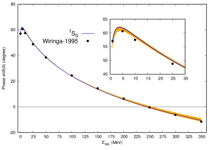
Figure 2: ${}^{1}S_{0}-nn$ SPS obtained through GOA (solid blue line) and CDA (yellow ribbon) analysis.

• By GOA we will be running 3 parameters ($V_{0},r_{m}\&a_{m}$) for all 11 SPS data points at once and obtain one set of globally optimized model parameters. This is shown by solid blue line in Figure 2.

• While by CDA we will be running 3 parameters for only 3 SPS data points. The CDA results creates a set of isospectral potential shown in Figure 2 as yellow bar.The details of the CDA procedure have been provided in the Appendix section 6.

2 Methodology:

The Morse function [10] is given by:

$$V_{\text{Morse}}(r)=V_{0}\left(e^{-2(r-r_{m})/a_{m}}-2e^{-(r-r_{m})/a_{m}}\right)$$ (1)

where the model parameters $V_{0}$, $r_{m}$ and $a_{m}$ reflect strength of interaction, equilibrium distance at which maximum attraction is felt (equilibrium separation) and range parameter respectively. It has all the interesting features that are observed in any typical scattering experiment, such as, strong repulsion at short distances, maximum attraction at an equilibrium distance $r_{m}$, followed by a quickly decaying tail at large distances. It can also be observed that realistic N-N interaction potentials, of Argonne v18 and Reid93 [8], for S-sates resemble that of a Morse function. Also, the phenomenological Malfeit-Tjohn potential [11] has a similar shape. Further, the analytical solution for the TISE with Morse potential interaction has already been solved for bound state energies ($E<0$) [12]. Hence, it can be considered as a good choice for modeling the interaction between any two scattering particles.

2.1 Phase Function Method:

The Schr$\ddot{o}$dinger wave equation for a spinless particle with energy E and orbital angular momentum $\ell$ undergoing scattering is given by

$$\frac{\hbar^{2}}{2\mu}\bigg{[}\frac{d^{2}}{dr^{2}}+\big{(}k^{2}-\ell(\ell+1)/r^{2}\big{)}\bigg{]}u_{\ell}(k,r)=V(r)u_{\ell}(k,r)$$ (2)

Where $k=\sqrt{E/(\hbar^{2}/2\mu)}$.

Second order differential equation Eq.2 has been transformed to the first order non-homogeneous differential equation of Riccati type [13, 14] given by following equation:

$$\delta_{\ell}^{\prime}(k,r)=-\frac{V(r)}{k}\bigg{[}\cos(\delta_{\ell}(k,r))\hat{j}_{\ell}(kr)-\sin(\delta_{\ell}(k,r))\hat{\eta}_{\ell}(kr)\bigg{]}^{2}$$ (3)

Here in Eq. 3 prime denotes differentiation of phase shift with respect to distance and the Riccati Hankel function of first kind is related to $\hat{j_{\ell}}(kr)$ and $\hat{\eta_{\ell}}(kr)$ by $\hat{h}_{\ell}(r)=-\hat{\eta}_{\ell}(r)+\textit{i}~{}\hat{j}_{\ell}(r)$ . In integral form the above equation can be simply written as:

$$\delta(k,r)=\frac{-1}{k}\int_{0}^{r}{V(r)}\bigg{[}\cos(\delta_{\ell}(k,r))\hat{j_{\ell}}(kr)-\sin(\delta_{\ell}(k,r))\hat{\eta_{\ell}}(kr)\bigg{]}^{2}dr$$ (4)

Eq.3 is numerically solved using Runge-Kutta 5^th order (RK-5) method with initial condition $\delta_{\ell}(0)=0$. For $\ell=0$, the Riccati-Bessel and Riccati-Neumann functions $\hat{j}_{0}$ and $\hat{\eta}_{0}$ get simplified as $\sin(kr)$ and $-\cos(kr)$, so Eq.3, for $\ell=0$ becomes

$$\delta^{\prime}_{0}(k,r)=-\frac{V(r)}{k}\sin^{2}[kr+\delta_{0}(k,r)]$$ (5)

The equation for amplitude function [15] with initial condition is obtained in the form

$$A_{\ell}^{\prime}(r)= -\frac{A_{\ell}V(r)}{k}\left[\cos(\delta_{\ell}(k,r))\hat{j}_{\ell}(kr)-\sin(\delta_{\ell}(k,r))\hat{\eta}_{\ell}(kr)\right]$$ (6)

$$\times\left[\sin(\delta_{\ell}(k,r))(\hat{j}_{\ell}(kr)+\cos(\delta_{\ell}(k,r))\hat{\eta}_{\ell}(kr)\right]$$

also the equation to obtained wavefunction [15] is

$$u_{\ell}(r)=A_{\ell}(r)\left[\cos(\delta_{\ell}(k,r))\hat{j}_{\ell}(kr)-\sin(\delta_{\ell}(k,r))\hat{\eta}_{\ell}(kr)\right]$$ (7)

In above equation the function $\delta_{0}(k,r)$ was termed “Phase function” by Morse and Allis [16]. The significant advantage of PFM method is that, the phase-shifts are directly expressed in terms of the potential and have no relation to the wavefunction. This has been utilised in this paper to obtain inverse potentials in an innovative way by implementing a modified VMC in tandem with PFM. The technique optimizes the model parameters of the potential to obtain the best match with respect to the experimental SPS values. Also, rather than solving the second order Schr$\ddot{o}$dinger equation, we only need to solve the first order non-homogeneous differential equation whose asymptotic value gives directly the value of SPS.

2.2 Optimization of Morse function model parameters using VMC:

Typically, VMC is utilized for obtaining the ground state energy for a given potential. The method initiates with a trial wavefunction, which is varied at a random location by a random amount in the Monte-Carlo sense. Then, the energy is determined using the newly obtained wavefunction and variational principle is applied. This process is done iteratively till one converges to the ground state. Here, we consider to vary the potential instead of wavefunction and minimise variance with respect to experimental data, as follows:
Initialisation step: To begin the optimisation procedure, Morse parameters $V_{0}$, $r_{m}$ and $a_{m}$ are given some initial values. The phase equation is integrated using RK-5 method for different values of $k$, a function of lab energies E, to obtain the simulated SPS, say $\delta^{sim}_{k}$. The mean percentage error (MPE) has been determined with respect to the SPS analysis data of Wiringa et al., [5], say $\delta^{exp}_{k}$, as

$$MPE=\frac{1}{N}\sum_{i=1}^{N}\frac{\lvert\delta^{exp}_{k}-\delta^{sim}_{k}\rvert}{\lvert\delta^{exp}_{k}\rvert}\times 100$$ (8)

This is named as $MPE_{old}$ and is also assigned to $MPE_{min}$.
Monte-Carlo step: A random number $r$, generated in an interval [-I, I], is added to one of the parameters, say $V_{0new}=V_{0}+r$.
PFM step: Again, the phase equation is integrated with new set of parameters $V_{0new}$, $r_{m}$ and $a_{m}$ to obtain new set of simulated scattering phase shifts (SPS), say $\delta^{sim-new}_{k}$, using which $MPE_{new}$ is determined.
Variational step: If $MPE_{new}<MPE_{old}$, then $V_{0}=V_{0new}$, $MPE_{min}=MPE_{new}$, else old values are retained.

The final three steps are repeated for each of the parameters to complete one iteration. The size of interval is reduced after a certain number of iterations, if there is no significant reduction in $MPE_{min}$. The process is completed when $MPE_{min}$ does not change any further, that is, convergence is reached.

3 Singlet Pseudo Bound S-wave Energy for nn

We know:

$$k\cot(\delta)=-\frac{1}{a}+\frac{1}{2}kr_{e}^{2}$$ (9)

where a and $r_{e}$ are scattering length and effective range. If use is made of the approximation specified by Eq. 9, the S matrix can be written in the form [3]:

$$S(k)=\left(\frac{k+i\alpha}{k-i\alpha}\right)\left(\frac{k+i\beta}{k-i\beta}\right)$$ (10)

Where S(k) is related to scattering length a and effective range $r_{e}$ by following relations

$$\alpha=\frac{1}{r_{e}}\bigg{[}1-\big{(}1-\frac{2r_{e}}{a}\big{)}^{1/2}\bigg{]}$$ (11)

$$\beta=\frac{1}{r_{e}}\bigg{[}1+\big{(}1-\frac{2r_{e}}{a}\big{)}^{1/2}\bigg{]}$$ (12)

The S matrix in Eq. 10 has two poles in the complex plane of the wave number k.

The first pole $i\beta$ ($\beta>0$), situated in the upper half-plane of k, is the well-known redundant pole of the S matrix. The second pole $i\alpha$ , situated in the lower half-plane of k, corresponds to a virtual ($i\alpha<0$) state of the two-nucleon system at the energy.

$$\epsilon=\frac{\hbar^{2}\alpha^{2}}{2m}$$ (13)

Using the obtained values for $a=-16.49(1.56)$ and $r_{e}=2.56(0.02)$ in Eq. 11 and then substituting the value in Eq. 13 the energy of the virtual ${}^{1}S_{0}-nn$ state comes out to be 0.135(22) MeV in comparison with $0.1293(158)$ given in [3].

4 Results and Discussion

At laboratory energies of nn scattering larger that $E_{\ell ab}=250MeV$ the measured scattering phase-shift in the ${}^{1}S_{0}$-wave interaction channel becomes negative, i.e., the interaction becomes repulsive. The fits to SPS are improved to reproduce the experimentally observed scattering length and effective range. To reproduce the observed negative S-wave phase shifts at higher energies with a static potential it is necessary to incorporate a repulsion into the potential. Here the Morse potential serves as a far more realistic potential in comparison to square well, exponential, Gaussian, or Hulthen potential used in the earlier studies. In addition to SPS and pseudo bound state energy for the nn system we have also obtained important quantum mechanical functions like (i) SPS vs. r(fm) (ii) Amplitude A(r) vs r(fm) and Wavefunction $u_{0}(r)$ for energy E=[5, 20, 50, 150, 250, 350]. These functions are shown in figure 3 respectively.

Table 1: Optimized parameters for ${}^{1}S_{0}-nn$ states using GOA and CDA. In later case, parameter values consisting of extreme depths are shown. Scattering length ($a$ in fm) and effective range ($r_{e}$ in fm) obtained, using SPS determined from these optimized parameters, are shown with experimental values (bold) [5] in curly brackets. Virtual ${}^{1}S_{0}$ state energy is taken from Petrov et al.

Analysis	$[V_{0}$, $r_{m}$, $a_{m}]$	MAE	$a(fm)$	$r_{e}(fm)$	$E_{nn}$
GOA	[67.523, 0.925, 0.376]	0.5	–17.64$\{$-18.5(0.4)$\}$	2.58$\{$2.8(0.11)$\}$	0.117{0.1293(158)}
CDA	[74.427,0.915,0.359]	0.7	-16.49(1.56)	2.56(0.02)	0.135(22){0.1293(158)}
	[65.191,0.915,0.381]	0.9

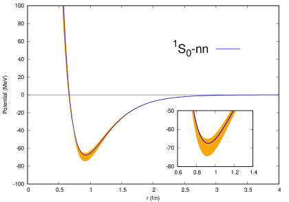
Figure 1: ${}^{1}S_{0}-nn$ potentilas obtained through GOA (solid blue line) and CDA (yellow ribbon) analysis.

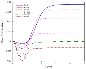
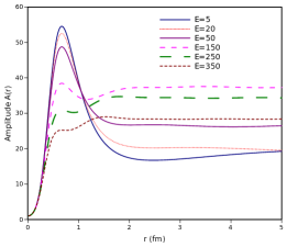
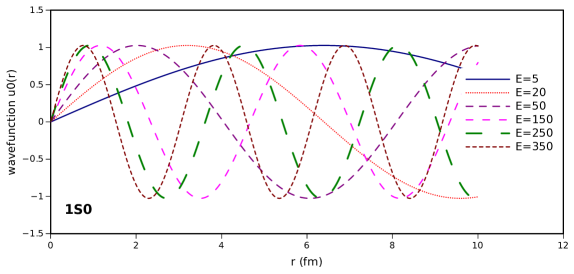
Figure 3: ${}^{1}S_{0}-nn$ SPS, amplitude and wavefunction function vs. distance r(fm) for ${}^{1}S_{0}-nn$ state.

5 Conclusion

The outcomes of the paper is: nn data from Wiringa et al. have been fitted to obtain the class of interaction potentials which further produces scattering parameters ($r_{e}$ and a) and pseudo bound state energy for the nn system. For this purpose we used VMC as an optimization procedure which was ran in tandem with phase function method. CDA (computationally time taking procedure $\approx$ 2,20,000 iterations) was performed to overcome the overfitting nature of GOA (less computational time $\approx$ 500 iterations) such that the class of potentials generated via CDA could give rise to the potentials which are capable in obtaining the low energy scattering parameters and energy. In addition we also obtained quantum mechanical functions like: amplitude and wavefunctions for nn interaction. We will be communicating GOA plus CDA for higher states of nn scattering in near future.

6 Appendix

6.1 Singlet State Analysis

• Since, we have three parameters to be determined for ${}^{1}S_{0}-nn$ state, a total of 165 combinations need to considered. All these are shown in Table LABEL:165combi, where the data have been once again presented in ascending order of overall MAE.

• Out of these 165, only 112 of them have $MAE<2$ (Table LABEL:165combi). The average value for $r_{m}$ from these 112 combinations is determined to be 0.915 fm.

• Keeping $r_{m}=0.915$ fixed, one needs to vary only two parameter $V_{0}$ and $a_{m}$. So, only ${}^{11}C_{2}$, that is 55 combinations need to be worked out. These are given in Table LABEL:55combi.

• A total of 21 combinations are having $MAE<1$. These have been considered for determining energy scattering parameters ($a_{s}$ and $r_{s}$) and are shown in Table LABEL:21combi.

• The values of depth $V_{0}$ and width $a_{m}$, given in bold (Table LABEL:21combi), are utilized for obtaining possible range of values for scattering parameters in our calculations.

Table 2: ${}^{1}S_{0}$ state: Model parameters for 165 combinations, each with three lab energies and obtained by minimising MSE. The overall MAE is determined by obtaining SPS for remaining experimental data points. The data is sorted with respect to MAE in ascending order.

Sr. No.	$E_{1}$ (MeV)	$E_{2}$ (MeV)	$E_{3}$ (MeV)	$V_{0}$ (MeV)	$r_{m}$ (fm)	$a_{m}$ (fm)	Overall MAE
1	5	100	300	77.115479	0.903579	0.350886	0.662538
2	5	100	250	74.794074	0.905138	0.356135	0.664066
3	5	50	250	66.555057	0.923181	0.377144	0.667124
4	5	50	300	68.714993	0.923036	0.371343	0.667529
5	1	50	250	63.920909	0.932580	0.386325	0.683027
6	1	50	300	66.096318	0.932593	0.380109	0.685002
7	1	100	250	72.609854	0.912592	0.363168	0.689700
8	1	100	300	74.974928	0.911009	0.357580	0.689736
9	5	100	350	78.975352	0.902434	0.346849	0.710647
10	5	150	250	80.031139	0.895761	0.344532	0.724937
11	5	100	200	72.078202	0.907161	0.362599	0.725451
12	5	150	300	82.482578	0.893344	0.339510	0.734344
13	1	100	350	76.876625	0.909845	0.353275	0.744264
14	5	150	200	77.282940	0.898713	0.350445	0.744734
15	5	50	350	70.484158	0.922960	0.366796	0.752458
16	1	100	200	69.825095	0.914668	0.370109	0.756181
17	1	150	250	78.083707	0.902422	0.350603	0.765884
18	5	150	350	84.381371	0.891599	0.335772	0.770784
19	5	50	200	63.979704	0.923428	0.384456	0.777142
20	1	150	300	80.592060	0.899901	0.345280	0.778598
21	1	50	350	67.882315	0.932638	0.375236	0.781104
22	5	200	250	83.695427	0.889976	0.337076	0.792821
23	5	25	250	59.371657	0.943254	0.399038	0.799728
24	1	50	200	61.317014	0.932620	0.394214	0.805355
25	5	25	300	61.414424	0.944445	0.392522	0.813973
26	1	150	350	82.547036	0.898076	0.341299	0.820508
27	5	200	300	86.368368	0.886791	0.331951	0.822296
28	10	50	250	69.079223	0.914998	0.369006	0.826098
29	10	50	300	71.223951	0.914683	0.363555	0.830384
30	1	25	250	56.293894	0.955358	0.410959	0.840832
31	1	200	250	81.911322	0.896193	0.342571	0.847136
32	5	200	350	88.277749	0.884659	0.328433	0.858753
33	1	25	300	58.320941	0.956947	0.403929	0.859694
34	5	100	150	68.510238	0.910179	0.371682	0.867157
35	10	100	250	76.890502	0.898528	0.349814	0.867544
36	10	100	300	79.172683	0.896958	0.344850	0.872223
37	10	25	250	62.328957	0.932878	0.388595	0.878832
38	1	200	300	84.642341	0.892865	0.337174	0.882417
39	10	25	300	64.384332	0.933691	0.382510	0.892251
40	10	50	350	72.976295	0.914475	0.359286	0.909298
41	1	100	150	66.168294	0.917781	0.379889	0.912405
42	10	100	200	74.240851	0.900538	0.355870	0.914718
43	5	250	300	89.779662	0.881551	0.325726	0.917400
44	10	50	200	66.533663	0.915464	0.375827	0.918218
45	10	100	350	80.993022	0.895804	0.341044	0.920199
46	1	200	350	86.617050	0.890615	0.333431	0.924701
47	10	150	250	81.907492	0.889782	0.339023	0.942778
48	5	25	200	56.917854	0.941723	0.407363	0.944494
49	5	25	350	63.104300	0.945385	0.387386	0.945559
50	10	150	200	79.250014	0.892611	0.344558	0.952231
51	5	250	350	91.482999	0.879424	0.322753	0.955824
52	10	150	300	84.307897	0.887426	0.334255	0.958265
53	1	250	300	88.148662	0.887337	0.330608	0.991374
54	10	150	350	86.153677	0.885734	0.330728	0.996277
55	1	25	200	53.855529	0.953255	0.419992	1.002329
56	10	25	200	59.867095	0.931867	0.396320	1.004255
57	10	25	350	66.079670	0.934349	0.377716	1.009266
58	1	25	350	60.000686	0.958187	0.398395	1.010507
59	10	200	250	85.417081	0.884354	0.332064	1.016014
60	5	300	350	93.552354	0.876249	0.319243	1.027944
61	10	100	150	70.755154	0.903526	0.364365	1.029546
62	1	250	350	89.938622	0.885053	0.327404	1.036422
63	5	50	150	60.654246	0.923860	0.394616	1.046363
64	10	200	300	88.041188	0.881264	0.327161	1.050844
65	10	200	350	89.885755	0.879225	0.323846	1.088957
66	5	10	250	52.061359	0.969479	0.426049	1.092622
67	1	50	150	57.955534	0.932734	0.405222	1.108618
68	1	300	350	92.123306	0.881627	0.323616	1.120125
69	5	10	300	53.988044	0.972202	0.418513	1.130341
70	10	50	150	63.245032	0.916219	0.385275	1.147237
71	10	250	300	91.366002	0.876248	0.321223	1.148571
72	10	250	350	92.984555	0.874252	0.318459	1.187414
73	1	10	250	48.534912	0.985705	0.441887	1.226465
74	10	300	350	94.940727	0.871296	0.315198	1.257704
75	5	10	200	49.742061	0.965777	0.435794	1.269821
76	1	10	300	50.407365	0.989203	0.433686	1.275819
77	25	50	250	74.165885	0.900566	0.354256	1.287763
78	25	50	300	76.288280	0.899839	0.349376	1.308031
79	5	10	350	55.591458	0.974292	0.412578	1.323138
80	5	25	150	53.769108	0.939484	0.418971	1.325565
81	10	25	150	56.704177	0.930439	0.407046	1.333711
82	25	50	200	71.675838	0.901540	0.360268	1.336092
83	25	50	350	78.008622	0.899316	0.345574	1.382325
84	1	10	200	46.281762	0.980843	0.452557	1.422110
85	1	150	200	101.253374	0.880595	0.309167	1.424588
86	1	25	150	50.732258	0.950087	0.432647	1.434219
87	25	50	150	68.456491	0.903012	0.368552	1.476343
88	25	100	250	81.169693	0.886459	0.338039	1.499279
89	1	10	350	51.971163	0.991852	0.427233	1.500739
90	25	100	200	78.640776	0.888565	0.343416	1.503322
91	25	100	300	83.385047	0.884770	0.333542	1.529394
92	1	5	250	44.703470	1.004339	0.460146	1.531274
93	25	100	150	75.299148	0.891671	0.350961	1.544265
94	5	50	100	56.161277	0.924590	0.409879	1.566059
95	10	50	100	58.818554	0.917491	0.399325	1.586276
96	25	100	350	85.132502	0.883530	0.330126	1.587127
97	1	5	300	46.491365	1.008976	0.451198	1.600957
98	25	150	200	83.291825	0.881340	0.333479	1.622311
99	25	150	250	85.776189	0.878634	0.328588	1.651279
100	25	150	300	88.087350	0.876299	0.324237	1.695171
101	1	50	100	53.407413	0.932875	0.421910	1.701221
102	1	5	200	42.555702	0.997748	0.471868	1.742130
103	25	50	100	64.168570	0.905385	0.380620	1.746915
104	25	150	350	89.830087	0.874644	0.321074	1.747854
105	25	200	250	88.985575	0.873745	0.322482	1.765219
106	5	10	150	46.786039	0.960056	0.449510	1.772808
107	25	200	300	91.528935	0.870731	0.317930	1.830865
108	1	5	350	47.990655	1.012439	0.444169	1.870402
109	25	200	350	93.247202	0.868811	0.314968	1.884770
110	25	250	300	94.707257	0.866003	0.312440	1.963546
111	1	10	150	43.425162	0.973119	0.467661	1.991153
112	10	25	100	52.429141	0.928047	0.423295	1.997752
113	25	250	350	96.143870	0.864233	0.310072	2.013517
114	25	300	350	97.857572	0.861669	0.307287	2.094282
115	5	25	100	49.514747	0.935561	0.436721	2.101010
116	50	100	250	85.638400	0.875559	0.327097	2.166302
117	50	100	300	87.817526	0.873615	0.322932	2.232250
118	50	100	350	89.496261	0.872214	0.319838	2.306645
119	1	25	100	46.523119	0.944299	0.452180	2.322517
120	50	150	200	87.586643	0.870942	0.322978	2.354390
121	1	5	150	39.854431	0.986974	0.488576	2.381987
122	50	150	250	89.892435	0.868248	0.318643	2.433698
123	50	150	300	92.144370	0.865792	0.314587	2.520239
124	50	150	350	93.782322	0.864105	0.311741	2.595768
125	50	200	250	92.796838	0.863730	0.313268	2.609630
126	50	200	300	95.310954	0.860607	0.308912	2.726528
127	50	200	350	96.894458	0.858748	0.306268	2.804948
128	5	10	100	42.834193	0.949276	0.470912	2.835505
129	50	250	300	98.394826	0.855944	0.303696	2.923710
130	50	250	350	99.610614	0.854397	0.301742	2.988923
131	50	300	350	101.038510	0.852221	0.299448	3.086309
132	1	10	100	39.645644	0.957950	0.491504	3.204863
133	100	150	200	93.222892	0.859267	0.310799	3.215942
134	100	150	250	95.213565	0.856649	0.307229	3.350851
135	10	25	50	45.667704	0.921380	0.454834	3.443735
136	100	150	300	97.445560	0.853883	0.303385	3.501372
137	100	200	250	97.627765	0.852638	0.302836	3.597631
138	100	150	350	98.929260	0.852136	0.300916	3.605990
139	1	5	100	36.346508	0.964850	0.515314	3.763530
140	100	200	300	100.240006	0.849066	0.298428	3.805282
141	5	25	50	42.830270	0.924177	0.471778	3.810106
142	100	200	350	101.632354	0.847259	0.296164	3.915039
143	150	200	250	100.455374	0.846841	0.297276	4.110838
144	100	250	300	103.385872	0.844043	0.293166	4.124725
145	100	250	350	104.197584	0.842930	0.291885	4.193478
146	100	300	350	105.126331	0.841428	0.290387	4.291667
147	1	25	50	39.988895	0.926528	0.491485	4.297531
148	150	200	300	103.488161	0.842317	0.292178	4.430524
149	150	200	350	104.716717	0.840585	0.290197	4.554876
150	150	250	300	107.091983	0.836250	0.286146	4.904307
151	150	300	350	107.712611	0.835260	0.285151	4.981076
152	250	300	350	108.438873	0.833609	0.283742	5.165724
153	5	10	50	36.900274	0.914826	0.515154	5.246407
154	200	300	350	109.443045	0.831385	0.281837	5.412344
155	200	250	350	110.400050	0.829656	0.280247	5.569773
156	200	250	300	111.292402	0.828317	0.278881	5.680566
157	1	10	50	34.242821	0.905331	0.542148	5.964818
158	1	5	50	31.855840	0.880018	0.574156	6.904728
159	5	10	25	33.160455	0.827556	0.571797	7.980513
160	1	10	25	32.404745	0.749428	0.610644	9.053548
161	1	5	25	35.401342	0.554285	0.660232	10.338711
162	1	5	10	60.167715	0.010001	0.707299	11.760083
163	50	100	200	21.505459	2.000000	1.357916	19.074560
164	50	100	150	18.792839	2.000000	1.460051	19.352376
165	150	250	350	39.237156	2.000000	1.232217	25.195640

Table 3: ${}^{1}S_{0}$ state: Model parameters for 55 combinations for ${}^{1}S_{0}-nn$ state. After fixing $r_{m}=0.9155$ (average) fm from 112 combinations of previous table LABEL:165combi, two parameters produces ${}^{11}C_{2}$ i.e. 55 combinations. The data is sorted with respect to MAE in ascending order.

Sr. No.	$E_{1}$ (MeV)	$E_{2}$ (MeV)	$V_{0}$ (MeV)	$a_{m}$ (fm)	Overall MAE
1	5	300	71.730802	0.363578	0.666437
2	5	250	69.812442	0.368384	0.666720
3	1	250	71.193511	0.366651	0.689214
4	1	300	72.930120	0.362403	0.689361
5	5	50	72.914193	0.360607	0.736652
6	5	350	73.343871	0.359686	0.738354
7	5	200	67.660861	0.374021	0.753482
8	1	350	74.427456	0.358861	0.754361
9	1	200	69.374385	0.371273	0.758771
10	50	300	70.968527	0.364323	0.814791
11	50	250	68.917538	0.369509	0.816551
12	100	200	69.587353	0.370934	0.817602
13	10	250	68.868276	0.369571	0.827726
14	10	300	70.898325	0.364391	0.833286
15	50	350	72.663694	0.360200	0.890809
16	100	150	66.847782	0.377443	0.900150
17	100	250	71.804840	0.365886	0.911899
18	10	350	72.583883	0.360260	0.914793
19	50	200	66.521411	0.375867	0.917600
20	10	200	66.517146	0.375874	0.918413
21	5	150	65.191362	0.380843	0.939942
22	100	300	73.759048	0.361589	1.044861
23	25	250	68.110429	0.370526	1.104946
24	25	300	70.216211	0.365056	1.122282
25	10	150	63.620993	0.384135	1.141107
26	5	100	63.240549	0.386527	1.142037
27	50	150	63.503218	0.384385	1.165667
28	25	200	65.625739	0.377329	1.190309
29	100	350	75.376753	0.358133	1.206715
30	25	350	71.951289	0.360735	1.217653
31	25	150	62.456573	0.386623	1.421515
32	50	100	59.621094	0.396317	1.614747
33	150	200	72.531742	0.366298	1.691748
34	25	100	58.241976	0.400252	1.876912
35	150	250	74.641661	0.362351	2.037006
36	150	300	76.578661	0.358811	2.376252
37	150	350	78.165101	0.355970	2.684166
38	10	50	101.859853	0.305723	2.942245
39	200	250	77.056751	0.359363	3.026641
40	200	300	79.074761	0.356343	3.612583
41	200	350	80.655030	0.354009	4.083227
42	10	25	42.587021	0.472826	4.263083
43	5	25	40.200809	0.489460	4.659452
44	250	300	81.441998	0.354000	4.800802
45	1	25	37.934492	0.507781	5.094683
46	5	10	36.968052	0.514500	5.213176
47	1	50	36.061249	0.523395	5.384020
48	250	350	82.929463	0.352199	5.389926
49	1	10	34.833315	0.534637	5.588524
50	1	5	32.866784	0.554584	5.952004
51	300	350	84.672221	0.350802	6.390542
52	25	50	30.513851	0.596846	7.700140
53	1	100	21.346168	0.752283	7.851272
54	10	100	18.349456	0.917733	9.809530
55	1	150	10.445956	1.341045	9.942812

Table 4: ${}^{1}S_{0}$ state: Model parameters for 21 combinations, each with three lab energies and obtained by minimising MSE. The overall MAE is determined by obtaining SPS for remaining experimental data points. The data is sorted with respect to $E_{1}$ in ascending order.

Sr. No.	$E_{1}$ (MeV)	$E_{2}$ (MeV)	$V_{0}$ (MeV)	$a_{m}$ (MeV)	Overall MAE	$r_{e}$ (fm)	$a$ (fm)
1	1	250	71.193511	0.366651	0.689214	-18.380	2.539
2	1	300	72.930120	0.362403	0.689361	-18.373	2.534
3	1	350	74.427456	0.358861	0.754361	-18.368	2.530
4	1	200	69.374385	0.371273	0.758771	-18.387	2.544
5	5	300	71.730802	0.363578	0.666437	-16.173	2.556
6	5	250	69.812442	0.368384	0.666720	-16.212	2.561
7	5	50	72.914193	0.360607	0.736652	-16.076	2.554
8	5	350	73.343871	0.359686	0.738354	-16.142	2.552
9	5	200	67.660861	0.374021	0.753482	-16.258	2.566
10	5	150	65.191362	0.380843	0.939942	-16.314	2.573
11	10	250	68.868276	0.369571	0.827726	-14.962	2.576
12	10	300	70.898325	0.364391	0.833286	-14.896	2.571
13	10	350	72.583883	0.360260	0.914793	-14.844	2.568
14	10	200	66.517146	0.375874	0.918413	-15.043	2.582
15	50	300	70.968527	0.364323	0.814791	-14.997	2.570
16	50	250	68.917538	0.369509	0.816551	-15.024	2.575
17	50	350	72.663694	0.360200	0.890809	-14.972	2.566
18	50	200	66.521411	0.375867	0.917600	-15.047	2.582
19	100	200	69.587353	0.370934	0.817602	-18.681	2.541
20	100	150	66.847782	0.377443	0.900150	-17.673	2.556
21	100	250	71.804840	0.365886	0.911899	-19.499	2.529
		Avg.	70.226561	0.367646	0.807472	-16.492	2.558
		St. Dev.	2.605663	0.006510	0.091322	1.557	0.017

References

- [1] Darewych, G. and Green, A.E.S., 1967. Morse Function and Velocity-Dependent Nucleon-Nucleon Potentials. Physical Review, 164(4), p.1324.
- [2] Henley, E.M. and Morrison, L.K., 1966. n-n and n-p Scattering Lengths and Charge Independence. Physical Review, 141(4), p.1489.
- [3] Babenko, V.A. and Petrov, N.M., 2016. Study of the low-energy characteristics of neutron-neutron scattering in the effective-range approximation. arXiv preprint arXiv:1605.04849.
- [4] Konobeevski, E., 2012, February. Study of Neutron-Neutron Scattering in nd Breakup Reaction. In Journal of Physics: Conference Series (Vol. 340, No. 1, p. 012047). IOP Publishing.
- [5] R.B. Wiringa, Stoks, V.G.J. and Schiavilla, R., 1995. Accurate nucleon-nucleon potential with charge-independence breaking. Physical Review C, 51(1), p.38.
- [6] Sastri, O.S.K.S., Khachi, A. and Kumar, L., 2022. An Innovative Approach to Construct Inverse Potentials Using Variational Monte-Carlo and Phase Function Method: Application to np and pp Scattering. Brazilian Journal of Physics, 52(2), p.58.
- [7] Khachi, A., Kumar, L. and Sastri, O.S.K.S., 2022. Alpha-Alpha Scattering Potentials for Various-Channels Using Phase Function Method. Physics of Atomic Nuclei, 85(4), pp.382-391.
- [8] Khachi, A., Kumar, L., Kumar, M.G. and Sastri, O.S.K.S., 2023. Deuteron structure and form factors: Using an inverse potential approach. Physical Review C, 107(6), p.064002.
- [9] Khachi, A., Kumar, L., Awasthi, A. and Sastri, O.S.K.S., 2023. Inverse potentials for all channels of neutron-proton scattering using reference potential approach. Physica Scripta, 98, 095301.
- [10] Morse, P.M., 1929. Diatomic molecules according to the wave mechanics. II. Vibrational levels. Physical review, 34(1), p.57.
- [11] Malfliet, R.A. and Tjon, J.A., 1969. Solution of the Faddeev equations for the triton problem using local two-particle interactions. Nuclear Physics A, 127(1), pp.161-168.
- [12] Matsumoto, A., 1988. Generalised matrix elements in discrete and continuum states for the Morse potential. Journal of Physics B: Atomic, Molecular and Optical Physics, 21(16), p.2863.
- [13] F. Calogero, Variable Phase Approach to Potential Scattering (Academic, New York, 1967)
- [14] V. Babikov, Uspekhi Fiz. Nauk 3, 92 (1967) https://doi.org/10.1070/PU1967v010n03ABEH003246
- [15] Zhaba, V.I., 2019. The variable phase approach: phase, amplitude and wave functions of the states for np-system for Argonne v18 potential. World Scientific News, (123), pp.161-180.
- [16] P.M. Morse, W.P. Allis, Phys. Rev. 44, 269 (1933) https://doi.org/10.1103/PhysRev.44.269