Using low-frequency scatter-broadening measurements for precision estimates of dispersion measures

Abstract

A pulsar’s pulse profile gets broadened at low frequencies due to dispersion along the line of sight or due to multi-path propagation. The dynamic nature of the interstellar medium makes both of these effects time-dependent and introduces slowly varying time delays in the measured times-of-arrival similar to those introduced by passing gravitational waves. In this article, we present a new method to correct for such delays by obtaining unbiased dispersion measure (DM) measurements by using low-frequency estimates of the scattering parameters. We evaluate this method by comparing the obtained DM estimates with those, where scatter-broadening is ignored using simulated data. A bias is seen in the estimated DMs for simulated data with pulse-broadening with a larger variability for a data set with a variable frequency scaling index, $\alpha$, as compared to that assuming a Kolmogorov turbulence. Application of the proposed method removes this bias robustly for data with band averaged signal-to-noise ratio larger than 100. We report, for the first time, the measurements of the scatter-broadening time and $\alpha$ from analysis of PSR J1643$-$1224, observed with upgraded Giant Metrewave Radio Telescope as part of the Indian Pulsar Timing Array experiment. These scattering parameters were found to vary with epoch and $\alpha$ was different from that expected for Kolmogorov turbulence. Finally, we present the DM time-series after application of the new technique to PSR J1643$-$1224.

1 Introduction

The precision in the time of arrival (ToA) of a pulsar’s radio pulse is determined in part by how bright and sharp the received pulse is. Both of these quantities, namely the signal-to-noise ratio (S/N) and the pulse width, are affected by the propagation of the pulsed signal through the ionised interstellar medium (IISM). The IISM can impose a frequency-dependent delay on the pulses, which, when added together without proper correction, will make the pulse appear smeared. This dispersion is mainly caused by the integrated column density of electrons along the line of sight and is quantified by the Dispersion Measure (DM). In addition, electron density inhomogeneities in the IISM encountered along the line of sight lead to multi-path propagation of radio waves, which also broadens the pulse (Rickett, 1977). This pulse broadening can be mathematically described as a convolution of the intrinsic pulse profile with a pulse broadening function, such as $\exp(-\phi/\tau_{sc})$, where $\phi$ is the pulse phase and $\tau_{sc}$ is the scatter-broadening time scale in the case of a thin scattering screen. Both of these phenomena are time-variable due to the dynamic nature of IISM. This variation induces a slowly varying chromatic time delay in the ToA measurements. The timescale of this stochastic delay is similar to that of the gravitational wave (GW) signature arising from an isotropic stochastic gravitational wave background (SGWB) formed by the random superposition of GWs emitted by an ensemble of super-massive black hole binaries (Burke-Spolaor et al., 2019). Hence, the wrong characterisation of this chromatic delay, or the individual pulsar chromatic noise, can lead to the false detection of SGWB (Zic et al., 2022).

The measurement and characterization of this IISM noise is therefore crucial for experiments, which use a collection of pulsars to observe the GW signal from SGWB (Srivastava et al., 2023). These experiments are called pulsar timing arrays (PTAs). There are four PTAs, which pool their data as part of the International Pulsar Timing Array consortium (IPTA : Hobbs et al., 2010; Verbiest et al., 2016) : the European Pulsar Timing Array (EPTA : Desvignes et al., 2016; Kramer & Champion, 2013), the Indo-Japanese pulsar timing array (InPTA : Joshi et al., 2018; Joshi et al., 2022; Tarafdar et al., 2022), the North American Nanohertz Observatory for Gravitational Waves (NANOGrav : McLaughlin, 2013) and the Parkes Pulsar Timing Array (PPTA : Manchester et al., 2013). Recently, the MeerKAT Pulsar Timing Array (MPTA : Miles et al., 2023; Bailes et al., 2020) and the Chinese Pulsar Timing Array (CPTA: Lee, 2016) have also started pulsar timing experiments.

The estimates of DM in these PTA experiments are usually obtained by quasi-simultaneous/simultaneous or even observations separated by few days, at two or three different observing frequencies (Arzoumanian et al., 2018; Tarafdar et al., 2022). The alignment of the fiducial point of the pulse at different observing frequencies is critical in such measurements. The scatter-broadening can introduce a systematic phase shift in the pulse’s fiducial point. In the measurement procedure, this needs to be accounted for to avoid a systematic bias in the measured DMs. Furthermore, slow variations in $\tau_{sc}$ over long periods of time can introduce corresponding variations in the measured DM values. Lastly, timing events, such as the ones reported in PSR J1713+0747 (Lam et al., 2018; Goncharov et al., 2020; Singha et al., 2021), produce a discontinuity in the Gaussian process DM models, if accompanied by changes in $\tau_{sc}$. These epoch dependent systematic errors in the DM estimates induce time varying delays in the ToAs, which act as a chromatic noise to SGWB signal. This noise, introduced by scatter-broadening variations, needs to be accounted for a reliable characterisation of the SGWB signal in PTA experiments. The correction of scatter-broadening in order to obtain robust estimates of DMs, and remove this noise is the primary motivation of this study.

The characterisation of scatter-broadening noise can be achieved with wide-band observations of millisecond pulsars (MSPs). Recently, wide-band receivers have been employed by the uGMRT ( 300-500 MHz : Gupta et al., 2017; Tarafdar et al., 2022), by the Parkes radio telescope (Hobbs et al., 2020, 800 $-$ 5000 MHz) and by CHIME (Amiri et al., 2021, 400 $-$ 800 MHz) for higher precision DM measurements. The scatter-broadening noise can be well characterized with such wide-band receivers. However, the dispersive delay due to the IISM varies as $f^{-2}$, whereas the pulse scatter-broadening evolves as $f^{-4.4}$ if a Kolmogorov turbulence is assumed in the IISM, where $f$ is the observational frequency (Rickett, 1977). This makes these propagation effects dominant at frequencies below 800 MHz, necessitating low-frequency measurements. If the scatter-broadening variations estimated from such observations can be removed from the data, robust and precision DM measurements can be obtained even for moderately high DM pulsars. In this paper, we present a new technique to achieve this and evaluate the efficacy of this technique using simulated data as well as data on a pulsar with significant pulse broadening.

The paper is arranged as follows. A new technique to remove the effect of pulse scatter-broadening is described in Section 2. The technique was tested first with simulated data with a known injection of DM and scatter-broadening variations, and the results are presented in Section 3. Results obtained by applying the technique on the InPTA data for PSR J1643$-$1224 are discussed in Section 4 followed by our conclusions in Section 5.

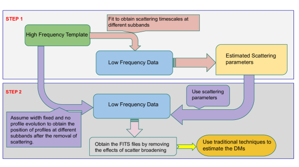
Figure 1: Schematic diagram of the technique for obtaining pulse profile by removing scatter-broadening using low-frequency observations.

2 Description of the new technique

Our new technique, which we call DMscat, makes use of the measurements of pulse broadening obtained using data between 300$-$500 MHz in order to recover the original pulse shape as best as possible. The procedure used in the technique is shown schematically in Figure 1. The pulse broadening measurements were obtained as follows. We use the frequency-resolved integrated pulse profiles with a chosen number of sub-bands between 300$-$500 MHz. The number of sub-bands was selected to obtain at least a 50 S/N pulse profile in each sub-band. Then, a template profile is generated from a high S/N pulse profile by collapsing the data at 1260$-$1460 MHz, where the pulse broadening is negligible. Next, this template is convolved with a pulse broadening function, $\exp({-\phi/\tau_{sc}})$. The convolved template is given by:

$$\mathcal{F}(\phi)=a\times s(\phi-b)*\exp(-\phi/\tau_{sc})\,,$$ (1)

where $s(\phi)$ is a high frequency template with amplitude $a$, $\phi$ is the pulse phase with peak at phase $b$, $\tau_{sc}$ is the pulse broadening time scale and $*$ denotes convolution. $\mathcal{F}(\phi)$ is then fitted to the observed pulse profile at each sub-band, keeping $\tau_{sc}$ as a fitted parameter, by minimizing the sum-of-squares of residuals obtained by subtracting the observed profile from $\mathcal{F}(\phi)$. This fit is carried out for each sub-band between 300$-$500 MHz data obtained using the InPTA observations and provides measurements of $\tau_{sc}$ as a function of observing frequency. The estimated $\tau_{sc}$ is then fitted to a power law model of the following form:

$$\tau_{sc}(f)=\tau_{0}f^{\alpha}$$ (2)

Here, $\tau_{0}$ is the pulse broadening at a reference frequency (e.g., 300 MHz) and $\alpha$ is the frequency scaling index of the scattering medium. This fit provides a measurement of $\alpha$ for each epoch.

Thereafter, these $\alpha$ measurements can be used to obtain the pulse profiles without scatter-broadening and therefore, provide more reliable measurements of DM. We use the same high-frequency template convolved with the scattering function, $\exp({-\phi/\tau_{sc}})$ but with the values of $\tau_{sc}$ estimated from the previous step to obtain a convolved profile, $T$. The sum-of-squared difference between the convolved profile and the observed scatter-broadened profile is given by:

$$\mathcal{R}^{2}=\sum(P_{i}-T_{i})^{2}\,,$$ (3)

where $P_{i}$ and $T_{i}$ are the $i$-th bin amplitudes of the observed scatter-broadened profile and convolved profile respectively. $R^{2}$ is minimized (least square minimization), keeping $\tau_{sc}$ fixed to the parameter estimated in the previous step and allowing the amplitude ($a$) and peak position ($b$) of the convolved pulse profile to vary. The residuals after the fitting are given by:

$$R_{i}=P_{i}-T_{i}.$$ (4)

For a good fit, $R_{i}$ is normally distributed and represents the noise in the profile.

Thus, the template profile, $s_{i}$, scaled by the amplitude at the fitted position provides a good representation of the pulse profile without scatter-broadening. This method is applied to all the sub-bands. and the obtained profiles are written back to a new PSRFITS file after adding the residuals, $R_{i}$ (noise), for each of the sub-bands. These profiles can now be used for estimating the DMs with conventional methods. It is important to note that the main assumption in these steps is that the profile of the pulsar does not evolve with frequency. While this may not hold true for most pulsars, a few of the MSPs monitored by PTAs do not show a strong frequency dependence.

3 Tests on Simulated Data

3.1 Simulations

We simulated frequency-resolved PSRFITS (Hotan et al., 2004) files using the parameter file of PSR J1643$-$1224 obtained from InPTA DR1 (Tarafdar et al., 2022). The primary objectives of our simulations were:

1. To gain an understanding of the impact of scatter-broadening on the DM estimation. Here, we explored two scenarios: one involved a scattering process characterised by the Kolmogorov turbulence spectrum ($\alpha=-4.4$) , and the other involved a scattering process with varying $\alpha$.

2. To validate and assess the efficacy of the DMscat software.

First, a single component pulse profile was simulated by generating a Gaussian placed at the middle of the pulse phase with a chosen width. For a given S/N across the band, the root mean square (RMS) of the required normally distributed noise was obtained by dividing the area under the pulse by the required S/N adjusted by the number of sub-bands. Noise with this RMS was then generated from a random number generator. This noise was added to each sub-band profile after convolving the pulse with the scatter-broadening function as described below. Data were simulated with S/N varying between 10 to 2000 (10, 20, 30, 50, 100, 400 and 2000).

We assumed a thin-screen model of the IISM (Williamson, 1972) to describe the scatter-broadening of the intrinsic pulse from the pulsar. The scattering timescale ($\tt\tau_{sc}$) is then calculated using

$$\log(\tau_{sc})=\log(\tau_{ref})+\alpha\times\log(f)-\alpha\times\log(300)\,,$$ (5)

where $f$ is the frequency, and $\tt\tau_{ref}$ is the pulse broadening at the reference frequency of 300 MHz. As explained later, we used both a constant $\alpha$ (-4.4) assuming the Kolmogorov spectrum as well as a variable $\alpha$. The simulated pulse was then convolved with the pulse broadening function, $\exp(-\phi/\tau_{sc})$ for each sub-band. Next, we generated the required noise for a given S/N as explained earlier and added this to the scattered pulse.

Then, we injected epoch to epoch DM variations using a DM time-series given as below:

$$DM(t)=DM_{0}+\delta DM(t-t_{0})^{3},$$ (6)

where $DM_{0}$ is the fiducial DM at $t_{0}$, chosen as the first epoch, over an observation interval spanning 10 years, sampled once every month. Three data sets with different amplitudes of DM variations, namely 0.01 (DMe-2), 0.001 (DMe-3), and 0.0001 (DMe-4) pc cm^-3, were generated. A phase delay corresponding to the simulated DM at a given epoch was calculated with phase predictors using TEMPO2 (Hobbs et al., 2006) for each sub-band, and the simulated and scattered pulse was placed at this phase delay by shifting it by the calculated delay. Finally, this frequency resolved simulated data were written to an output PSRFITS file.

For each amplitude of the DM variation, three sets of simulated data were produced. The first set of simulated data had only the DM variation with no scatter-broadening (NS case). In the second set of simulated data, along with the DM variations, we also incorporated scatter-broadening effect with a constant value of the frequency scaling index, $\alpha=-4.4$, assuming a Kolmogorov turbulence (CS case). The value of $\tau$ at 300 MHz was chosen to be 0.7 ms. In the third set, along with the DM variations, we incorporated a variation in the frequency scaling index, $\alpha$ (VS case). Here, we used the measurements of frequency scaling index, $\alpha$ for PSR J1643$-$1224 as the injected $\alpha$. The value of $\tau$ at 300 MHz was fixed for all the profiles and scaled accordingly with the frequency. Thus, we simulated 21 data-sets, each with 120 epochs, for the three different cases.

First, the simulated data-sets were used to understand the effect of scatter-broadening on the estimates of DM. Then, our new technique was tested and evaluated on the simulated data for CS and VS cases. The results of these analyses are presented in the following sections.

3.2 Effect of scatter-broadening on DM Estimates

We used DMCalc (Krishnakumar et al., 2021) on these simulated pulsar profiles to estimate the DMs for all the cases. In order to run DMCalc, we selected a high S/N ratio (from the 2000 S/N case) template for each case. The DMs were estimated for the simulated data-sets spanning the range of S/N for all the three cases: NS, CS and VS. The results are presented in Figure 2, where the plots of estimated DMs are shown after subtracting the injected DMs for simulated data-sets with S/N equal to 20 and 400, and the amplitude of DM variations equal to 0.0001. The mean difference between the estimated and the injected DMs over all epochs and its standard deviation are also listed in the third and fifth columns of Table 1, respectively. The DM errors are plotted in the top panel of Figure 4.

As the pulse is without scatter-broadening in the NS case, the estimated DMs were consistent with the injected DMs for the full range of S/N, with the mean difference smaller than the DM error. In the CS and VS cases, where the simulated data-set consists of scatter-broadened pulse, the DMs were estimated with a bias, seen as offsets in Figure 2 and significant mean difference in Table 1. The bias is smaller for the VS case than for the CS case. While these results hold for different S/N, the median uncertainty in the estimated DMs varies with S/N as expected. This variation is shown in Figure 4. While the median DM error increases with decreasing S/N below S/N of 50, the median DM error is almost the same for S/N greater than 50. The median DM error was larger for VS as compared to the CS case for S/N less than 50.

The standard deviation in Table 1 gives an idea of the variability in the DM estimates over all the epochs. The estimated DMs had larger variability for cases with S/N less than 50. Another interesting feature in our results is that the variability was larger for the VS case as compared to the CS case, suggesting a larger fluctuation of DM estimates for pulsars showing variable scatter-broadening with observation epochs. These trends were consistent for all cases of DM variations.

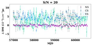
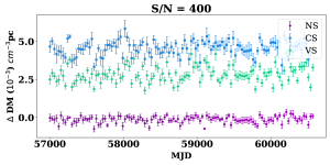
Figure 2: The difference between injected and estimated DMs ($\Delta$ DM) for three cases: no scattering (NS), constant scattering (CS), and variable scattering (VS) for the set of files generated with S/N = 20 (upper panel) and 400 (lower panel) with injected DM variations of the order 0.0001 cm^-3 pc. These measurements were carried out on the simulated data before the application of DMscat.

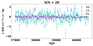
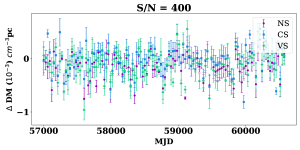
Figure 3: The difference between the injected and estimated DMs ($\Delta$ DM) for three cases: no scattering (NS), constant scattering (CS), and variable scattering (VS) for the set of files generated with S/N = 20 (upper panel) and 400 (lower panel) with injected DM variations of the order 0.0001 cm^-3 pc. These measurements were carried out on the simulated data after the application of DMscat .

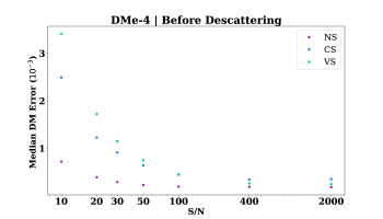
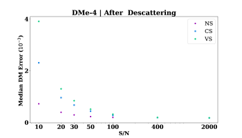
Figure 4: The variation of median error in the DM estimation with respect to S/N before (upper panel) and after (lower panel) the application of DMscat.

3.3 Testing DMscat on simulated data

We used the simulated data sets in order to demonstrate and test our new method of removing the effect of scatter-broadening on the DM estimates. We tested DMscat on the CS and VS datasets to generate new pulse profiles. First, we compared the recovered profiles for each sub-band against the injected profiles by subtracting the recovered profile from the injected profile. The obtained residuals were normally distributed and consistent with the noise injected in the simulated data demonstrating that the technique works well on the simulated data, particularly for S/N greater than 100. The technique worked for both CS and VS cases for different DM variations.

Then, we used DMCalc on these new profiles to estimate the DMs. The results are shown in Figure 3, where plots of the estimated DMs are shown after subtracting the injected DMs for the simulated data-set with S/N equal to 20 and 400 and amplitude of DM variations equal to 0.0001. The mean difference between the estimated and the injected DMs over all epochs and their standard deviations are also listed in the fourth and sixth columns of Table 1. Broadly, the mean of the estimated DMs for the CS and VS cases were consistent with the ones obtained for the NS case, while the variability, reflected by the standard deviation was larger for CS and VS cases as compared to the NS case.

The estimated and the injected DMs were consistent within the DM errors for both CS and VS cases for all S/N cases, as is evident from Table 1, indicating that the technique is able to recover the injected DMs without the bias seen in the scatter-broadened data. Moreover, the variability of DM estimates over epochs is reduced by about half for S/N above 100, whereas the variability is the same or worse for S/N below 100. This validates DMscat and suggests that the technique will be useful in reducing the scatter-broadening noise for S/N larger than 100.

The two panels of Figure 4 compare the median DM errors before and after the application of DMscat. After the application of DMscat, the median DM error is similar for NS, CS, and VS cases with S/N larger than 100, whereas for data-sets with S/N lower than 100, the median error does not seem to improve. This again suggests that the new technique will work optimally for the datasets with S/N higher than 100.

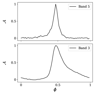
Figure 5: Plots showing the scatter-broadening in PSR J1643$-$1224 in Band 3 (lower panel) and a sharp profile with negligible scattering in Band 5 (upper panel). Here $\mathcal{A}$ is the amplitude (in arbitrary units) and $\phi$ is the pulse phase.

Table 1: The values of mean and standard deviations of the differences of injected versus estimated DMs for various cases with different S/N for the simulations with DM variation of the order 0.0001.

S/N value	Cases	Mean (10-3) cm-3 pc		Standard Deviation (10-3) cm-3 pc
		Before	After	Before	After
10	NS	0.015		0.37
	CS	4.8	-0.46	4.5	4.6
	VS	5.7	-2.4	10.5	11.6
20	NS	-0.10		0.41
	CS	4.4	0.16	1.8	1.7
	VS	2.5	-0.31	2.5	2.1
30	NS	-0.11		0.30
	CS	4.3	-0.016	1.1	1.0
	VS	2.4	-0.42	1.7	1.2
50	NS	-0.11		0.23
	CS	4.3	-0.0032	0.69	0.63
	VS	2.5	-0.24	1.0	0.79
100	NS	-0.13		0.22
	CS	4.5	-0.0097	0.48	0.35
	VS	2.6	-0.17	0.68	0.43
400	NS	-0.13		0.21
	CS	4.5	-0.026	0.46	0.23
	VS	2.8	-0.11	0.51	0.25
2000	NS	-0.11		0.21
	CS	4.5	-0.018	0.48	0.22
	VS	2.8	-0.083	0.5	0.22

4 Application of DMscat on PSR J1643-1224

After validating DMscat, we applied this technique on PSR J1643$-$1224 data observed with the uGMRT as part of the InPTA observations. PSR J1643$-$1224 is a pulsar in the PTA ensemble that exhibits prominent scatter-broadening. This pulsar is observed in the InPTA experiment simultaneously at two different frequency bands, namely Band 3 (300$-$500 MHz) and Band 5 (1260$-$1460 MHz), using the upgraded Giant Metrewave Radio Telescope (Gupta et al., 2017; Reddy et al., 2017). These simultaneous observations at two different bands allow us to estimate the DMs with high precision. Negligible scatter-broadening is seen in Band 5 data, whereas the pulsar shows significant pulse broadening at Band 3 as can be seen in Fig. 5. We used the observations over two years between 2019 to 2021, which also formed part of InPTA Data Release 1 (InPTA-DR1 : Tarafdar et al., 2022). We only used the data observed with 200 MHz bandwidth (MJD 58781 $-$ 59496). The DM time series of this pulsar, obtained with DMCalc using data without accounting for scatter-broadening, were presented in the InPTA-DR1 and is shown in Figure 8.

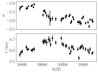
Figure 6: Upper panel:The estimated scatter-broadening time ($\tau_{sc}$ at 406 MHZ, near the band centre) data for PSR J1643$-$1224 is shown as a function of observing epoch. Lower panel: The frequency scaling index ($\alpha$ over Band 3 is plotted in this figure for PSR J1643$-$1224 over 2019 to 2021

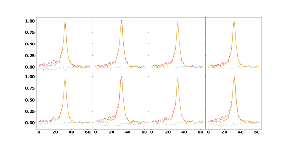
Figure 7: The figure shows the comparison of the reconstructed profile in Band 3 with respect to the Band 5 template which was used to descatter the profile. The solid curve in yellow indicates the Band 5 template, the red dashed curve shows the Band 3 profile after removing scattering, with the assumption that the profile does not evolve with frequency. The blue dotted curve indicates the residuals, i.e., the difference between the template and the Band 3 profile at every frequency channel.

First, the Band 5 data for PSR J1643$-$1224 were collapsed across the band to obtain a template for the highest S/N epoch (MJD 59032). Band 3 data were collapsed to 16 sub-bands. Then, we obtained the estimates of $\tau_{sc}$ for each of the 16 sub-bands and $\alpha$ as described in Section 2. These are presented in Figures 6. Significant variations are seen in both the parameters over the 2 year time-scale of the data, which suggests that DM estimates are likely to have a time-varying bias due to scatter-broadening. This, coupled with epoch-dependent time delays due to scatter-broadening itself needs to be accounted for in this pulsar for a meaningful GW analysis. Further, the median frequency scaling index was estimated to be -2.84, which was different from Kolmogorov turbulence (-4.4).

We used the estimates of $\tau_{sc}$ and $\alpha$ presented in Figures 6 to remove scatter-broadening in the pulse using DMscat as explained in Section 2. We show a comparison of the Band 3 reconstructed profiles at different frequency channels with the Band 5 template for MJD 59015 in Figure 7. The residuals obtained by subtracting the two profiles at every sub-band are also shown in this figure. Application of the Anderson-Darling test (Anderson & Darling, 1952) shows that these residuals were normally distributed. Therefore, DMscat is able to recover the profile without scatter-broadening.

The resultant PSRFITS files were analysed with DMCalc to estimate the DMs. The estimated DMs after the application of DMscat are shown in Figure 8 along with the DM obtained in InPTA-DR1.

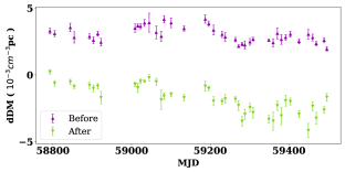
Figure 8: The DM time series for the InPTA dataset of PSR J1643$-$1224 before and after the application of the new technique. Here, dDM is the offset between the estimated and the fiducial DM used to align the template.

5 Conclusions

In this paper, we have demonstrated that the pulse-broadening in pulsar data can affect the estimates of DM using wide-band observations. Using simulated data, we show that a bias is seen in the DM estimates in scatter-broadened data. This bias depends on the spectral index of turbulence. The variability of the DM estimates over different epochs was found to be larger for scattering with a variable $\alpha$ suggesting that the DM noise estimates may be less reliable for scattering with a variable $\alpha$. A new technique, DMscat, for removing the pulse-broadening due to multi-path propagation in the IISM is presented in this paper to remove the observed bias. The technique was validated with tests on simulated data, where it was shown that the estimated DMs are consistent with the injected ones. The median DM error on the recovered DMs for the scattered data were shown to be similar to those for the data without scattering for S/N larger than 100. This suggests that the technique will be useful in reducing the scattering noise for S/N larger than 100. The measurements of the frequency scaling index, $\alpha$, and scatter-broadening time, $\tau_{sc}$, were presented for the first time for PSR J1643$-$1224 observed using the uGMRT as part of the InPTA project. Both $\alpha$ and $\tau_{sc}$ were found to vary with observational epochs and $\alpha$ was measured to be different from that expected for a medium with Kolmogorov turbulence. DMscat was applied to PSR J1643$-$1224 to obtain a DM time-series from profiles without pulse-broadening. Thus, we have demonstrated the applicability of DMscat both on simulated data-sets and observed pulsar data under the assumption that there is negligible frequency evolution of profile.

A few pulsars amongst the PTA sample, such as PSRs J1643$-$1224 and J1939+2134, show significant DM variations as well as scatter-broadening at low frequencies. While these are bright pulsars with a high potential for precision timing, the variation in the ToA delays due to scattering most likely limits their contribution to a PTA experiment. Typically, such IISM variations are removed from timing residuals by modeling these chromatic noise sources as Gaussian processes (GP). In most of the recent PTA work, the IISM noise is modeled as a DM GP process with a $\nu^{-2}$ dependence (Srivastava et al., 2023). The presence of scattering can lead to a leakage of the IISM noise in achromatic noise models, which can introduce subtle systematic in decade long PTA data-sets, particularly when the time scale of such chromatic variations are similar to achromatic or deterministic variations. An analysis after the application of DMscat can potentially help in the robust determination of these models at least for PSR J1643$-$1224. We intend to carry out such analysis as a follow-up work.

The main limitation of the method is that it may not work when frequency evolution of the profiles is present. Techniques to address this limitation are motivated by this work. Possibilities are a modification of wide-band techniques (Pennucci et al., 2014; Nobleson et al., 2022; Paladi et al., 2023) or CLEAN based techniques (Bhat et al., 2003). Such developments are intended in the near future, which could be tested on the simulated data as well as actual observations.

With the recently announced evidence for GW signal from GWB (Agazie et al., 2023; Antoniadis et al., 2023; Reardon et al., 2023; Xu et al., 2023), the development of methods such as DMscat is important not only to increase the significance of the signal in the upcoming IPTA Data Release 3, but also to constrain the new physics, which can be investigated by this ultra-low wavelength window of GW astronomy.

Data Availability

The data underlying this article will be shared on reasonable request to the corresponding author.

Software

DSPSR (van Straten & Bailes, 2011), PSRCHIVE (Hotan et al., 2004), RFIClean (Maan et al., 2021), PINTA (Susobhanan et al., 2021), TEMPO2 (Hobbs et al., 2006; Edwards et al., 2006), DMCALC (Krishnakumar et al., 2021), lmfit (Newville et al., 2014), matplotlib (Hunter, 2007), astropy (Price-Whelan et al., 2018).

Affiliations

¹High Energy Physics, Cosmology & Astrophysics Theory (HEPCAT) Group, Department of Mathematics and Applied Mathematics,
University of Cape Town, Cape Town 7700, South Africa
²Department of Physics, Indian Institute of Technology Roorkee, Roorkee 247667, Uttarakhand, India
³National Centre for Radio Astrophysics, Tata Institute of Fundamental Research, Pune 411007, Maharashtra, India
⁴Max-Planck-Institut für Radioastronomie, Auf dem Hügel 69, 53121 Bonn, Germany
⁵Fakultät für Physik, Universität Bielefeld, Postfach 100131, 33501 Bielefeld, Germany
⁶Department of Physical Sciences, IISER Kolkata, West Bengal, India
⁷Center of Excellence in Space Sciences India, IISER Kolkata, West Bengal, India
⁸Indian Institute of Science Education and Research, Mohali, 140306, India
⁹Department of Earth and Space Sciences, Indian Institute of Space Science and Technology, Valiamala P.O., Thiruvananthapuram 695547, Kerala, India
¹⁰Department of Physics, Government Brennen College, Thalassery, Kannur University, Kannur 670106, Kerala, India
¹¹Department of Physics, IIT Hyderabad, Kandi, Telangana 502284
¹²The Institute of Mathematical Sciences, C. I. T. Campus, Taramani, Chennai 600113, India
¹³Department of Electrical Engineering, IIT Hyderabad, Kandi, Telangana 502284, India
¹⁴Homi Bhabha National Institute, Training School Complex, Anushakti Nagar, Mumbai 400094, India
¹⁵Department of Physics and Astrphysics, Delhi University, Delhi, India
¹⁶Department of Astronomy and Astrophysics, Tata Institute of Fundamental Research, Homi Bhabha Road, Navy Nagar, Colaba, Mumbai 400005, India
¹⁷International Research Organization for Advanced Science and Technology, Kumamoto University, 2-39-1 Kurokami, Kumamoto 860-8555, Japan
¹⁸Osaka Central Advanced Mathematical Institute, Osaka Metropolitan University, Osaka, 5588585, Japan
¹⁹Faculty of Advanced Science and Technology, Kumamoto University, 2-39-1 Kurokami, Kumamoto 860-8555, Japan
²⁰Kumamoto University, Graduate School of Science and Technology, Kumamoto, 860-8555, Japan
²¹Australia Telescope National Facility, CSIRO, Space and Astronomy, PO Box 76, Epping, NSW 1710, Australia
²²Birla Institute of Technology & Science, Pilani Hyderabad
²³Joint Astronomy Programme, Indian Institute of Science, Bengaluru, Karnataka, 560012, India
²⁴Raman Research Institute, Bangalore, 560080, India
²⁵Department of Physics, Indian Institute of Science Education and Research Bhopal, Bhopal Bypass Road, Bhauri, Bhopal 462 066, Madhya Pradesh, India
²⁶Center for Gravitation Cosmology and Astrophysics, University of Wisconsin-Milwaukee, Milwaukee, WI 53211, USA

References

- Agazie et al. (2023) Agazie G., et al., 2023, The Astrophysical Journal Letters, 951, L8
- Amiri et al. (2021) Amiri M., et al., 2021, The Astrophysical Journal Supplement Series, 255, 5
- Anderson & Darling (1952) Anderson T. W., Darling D. A., 1952, The Annals of Mathematical Statistics, 23, 193
- Antoniadis et al. (2023) Antoniadis J., et al., 2023, arXiv e-prints, p. arXiv:2306.16214
- Arzoumanian et al. (2018) Arzoumanian Z., et al., 2018, The Astrophysical Journal Supplement Series, 235, 37
- Bailes et al. (2020) Bailes M., et al., 2020, Publ. Astron. Soc. Australia, 37, e028
- Bhat et al. (2003) Bhat N. D. R., Cordes J. M., Chatterjee S., 2003, ApJ, 584, 782
- Burke-Spolaor et al. (2019) Burke-Spolaor S., et al., 2019, A&ARv, 27, 5
- Desvignes et al. (2016) Desvignes G., et al., 2016, MNRAS, 458, 3341
- Edwards et al. (2006) Edwards R. T., Hobbs G. B., Manchester R. N., 2006, Monthly Notices of the Royal Astronomical Society, 372, 1549
- Goncharov et al. (2020) Goncharov B., et al., 2020, Monthly Notices of the Royal Astronomical Society, 502, 478
- Gupta et al. (2017) Gupta Y., et al., 2017, Current Science, 113, 707
- Hobbs et al. (2006) Hobbs G. B., Edwards R. T., Manchester R. N., 2006, Monthly Notices of the Royal Astronomical Society, 369, 655
- Hobbs et al. (2010) Hobbs G., et al., 2010, Classical and Quantum Gravity, 27, 084013
- Hobbs et al. (2020) Hobbs G., et al., 2020, Publications of the Astronomical Society of Australia, 37, e012
- Hotan et al. (2004) Hotan A. W., van Straten W., Manchester R. N., 2004, Publications of the Astronomical Society of Australia, 21, 302
- Hunter (2007) Hunter J. D., 2007, Computing in Science & Engineering, 9, 90
- Joshi et al. (2018) Joshi B. C., et al., 2018, Journal of Astrophysics and Astronomy, 39, 51
- Joshi et al. (2022) Joshi B. C., Gopakumar A., Pandian A., et al., 2022, Journal of Astrophysics and Astronomy, 10
- Kramer & Champion (2013) Kramer M., Champion D. J., 2013, Classical and Quantum Gravity, 30, 224009
- Krishnakumar et al. (2021) Krishnakumar M. A., et al., 2021, Astronomy & Astrophysics, 651, A5
- Lam et al. (2018) Lam M. T., et al., 2018, ApJ, 861, 132
- Lee (2016) Lee K. J., 2016, in Qain L., Li D., eds, Astronomical Society of the Pacific Conference Series Vol. 502, Frontiers in Radio Astronomy and FAST Early Sciences Symposium 2015. Astronomical Society of the Pacific, p. 19, http://www.aspbooks.org/a/volumes/ARTICLE_details/?paper_id=37688
- Maan et al. (2021) Maan Y., van Leeuwen J., Vohl D., 2021, Astronomy & Astrophysics, 650, A80
- Manchester et al. (2013) Manchester R. N., et al., 2013, Publ. Astron. Soc. Australia, 30, e017
- McLaughlin (2013) McLaughlin M. A., 2013, Classical and Quantum Gravity, 30, 224008
- Miles et al. (2023) Miles M. T., et al., 2023, MNRAS, 519, 3976
- Newville et al. (2014) Newville M., Stensitzki T., Allen D. B., Ingargiola A., 2014, LMFIT: Non-Linear Least-Square Minimization and Curve-Fitting for Python, doi:10.5281/zenodo.11813, https://doi.org/10.5281/zenodo.11813
- Nobleson et al. (2022) Nobleson K., et al., 2022, Monthly Notices of the Royal Astronomical Society, 512, 1234
- Paladi et al. (2023) Paladi A. K., et al., 2023, arXiv e-prints, p. arXiv:2304.13072
- Pennucci et al. (2014) Pennucci T. T., Demorest P. B., Ransom S. M., 2014, The Astrophysical Journal, 790, 93
- Price-Whelan et al. (2018) Price-Whelan A. M., et al., 2018, AJ, 156, 123
- Reardon et al. (2023) Reardon D. J., et al., 2023, The Astrophysical Journal Letters, 951, L6
- Reddy et al. (2017) Reddy S. H., et al., 2017, Journal of Astronomical Instrumentation, 6, 1641011
- Rickett (1977) Rickett B. J., 1977, ARA&A, 15, 479
- Singha et al. (2021) Singha J., et al., 2021, Monthly Notices of the Royal Astronomical Society: Letters, 507, L57
- Srivastava et al. (2023) Srivastava A., et al., 2023, Phys. Rev. D, 108, 023008
- Susobhanan et al. (2021) Susobhanan A., et al., 2021, Publications of the Astronomical Society of Australia, 38, e017
- Tarafdar et al. (2022) Tarafdar P., et al., 2022, Publications of the Astronomical Society of Australia, 39, e053
- Verbiest et al. (2016) Verbiest J. P. W., et al., 2016, Monthly Notices of the Royal Astronomical Society, 458, 1267
- Williamson (1972) Williamson I. P., 1972, MNRAS, 157, 55
- Xu et al. (2023) Xu H., et al., 2023, Research in Astronomy and Astrophysics, 23, 075024
- Zic et al. (2022) Zic A., et al., 2022, MNRAS, 516, 410
- van Straten & Bailes (2011) van Straten W., Bailes M., 2011, Publications of the Astronomical Society of Australia, 28, 1