Memory in Plain Sight
A Survey of the Uncanny Resemblances between Diffusion Models and Associative Memories

Abstract

Diffusion Models (DMs) have recently set state-of-the-art on many generation benchmarks. However, there are myriad ways to describe them mathematically, which makes it difficult to develop a simple understanding of how they work. In this survey, we provide a concise overview of DMs from the perspective of dynamical systems and Ordinary Differential Equations (ODEs) which exposes a mathematical connection to the highly related yet often overlooked class of energy-based models, called Associative Memories (AMs). Energy-based AMs are a theoretical framework that behave much like denoising DMs, but they enable us to directly compute a Lyapunov energy function on which we can perform gradient descent to denoise data. We then summarize the 40 year history of energy-based AMs, beginning with the original Hopfield Network, and discuss new research directions for AMs and DMs that are revealed by characterizing the extent of their similarities and differences.

1 Introduction

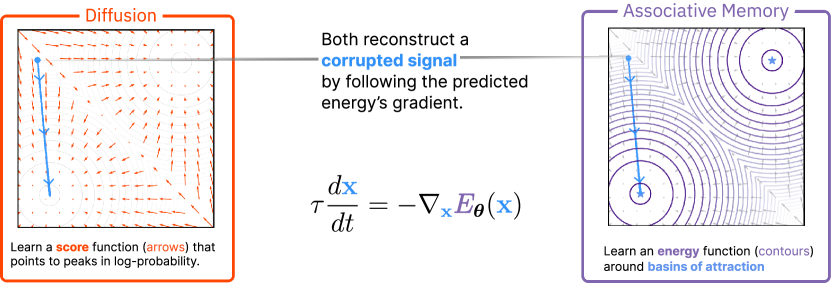
Figure 1: Comparing the emphases of Diffusion Models and Associative Memories tasked with learning the same energy (negative log-probability) landscape, represented with both contours and gradient arrows. Diffusion Models (left) train a score function (depicted as orange arrows) to model the gradient of the energy. The noisy starting signal (depicted as a blue circle) becomes less corrupted by following these gradients in the reverse denoising process. Associative Memories (right) instead learn a smooth energy function, depicted as contours. The “memory retrieval dynamics” is the process by which a fixed point is retrieved by following the energy gradient from the initial signal. This process is mathematically equivalent to the objective of the reverse denoising process of Diffusion Models. Memory retrieval dynamics always converge to fixed points (there are two in the figure, the top right and lower left) where the energy is at a local minimum. This guarantee does not exist for Diffusion Models.

Diffusion Models [1, 2, 3, 4] (DMs) have rapidly become the most perfomant class of generative models on images [5, 6, 7, 8, 9]. Recent examples of well known DMs include Imagen [7] (backed by Google), DALLE-2 [6] (backed by OpenAI), Midjourney [10] (an independent research lab), and Stable Diffusion [8] (backed by StabilityAI). The strong adoption of DMs by large companies, startups, and academia continue to lower the computational barriers to these models and push the capabilities of these models to domains like videos [11], molecules [12], audio [13, 14, 15], and even text [16].

On each of these domains, a trained DM will use a neural network to iteratively denoise a noisy image (or other data point) until there is no noise remaining. Each denoising step aims to increase the probability (specifically, the log-probability) that the noisy data looks like a sample from the real data distribution. An example log-probability landscape with two peaks of “real-looking data” (located at the top right and bottom left of the landscape) is shown in the left half of Figure 1, where each denoising step pushes the initial noisy image (blue dot) towards regions of higher log-probability.

The overall goal of a DM is to repeatedly denoise an image until no noise remains. That is:

Goal of Diffusion Models: Given a corrupted representation of some data, recreate the original uncorrupted data.

However, this is not how diffusion processes behave in non-equilibrium thermodynamics [1]. Consider an example of diffusion in nature, where a droplet of red food dye is dropped into a glass of hot water. The millions of tiny red particles in the droplet rapidly “diffuse” through the water away from its initial concentration until the resultant water is a uniformly pale pink. We can say that diffusion is then an inherently information-destroying process in forward time; one which maximizes the entropy of a distribution of particles.

If diffusion is information-destroying, then training a neural network to reverse this process must be information-adding. This is the essence of DMs as proposed by [1, 2]. The forward process of DMs iteratively adds noise to some image (or other data), whereas the reverse process is trained to remove the noise introduced at each step of the forward process in an attempt to recreate the original image. The forward process on its own is un-parameterized and non-interesting, only requiring that the added noise intelligently explores all important regions of the log-probability landscape; the computational power of Diffusion Models lies entirely in its reverse process.

1.1 Diffusion’s Unseen Connection to Associative Memories

Associative Memory (AM) is a theory for the computational operation of brains that originated in the field of psychology in the late 19th century [17]. We are all familiar with this phenomenon. Consider walking into a kitchen and smelling a freshly baked apple pie. The smell could elicit strong feelings of nostalgia and festivities at grandma’s, which surfaces memories of the names and faces of family gathered for the holidays. The smell (query) retrieved a set of feelings, names, and faces (values) from your brain (the associative memory).

Formally, AMs are dynamical systems that are concerned with the storage and retrieval of data (a.k.a. signals) called memories [18]. These memories live at local minima of an energy landscape that also includes all possible corruptions of those memories. From the Boltzmann distribution (Eq. 1), we know that energy can be understood as a negative and unscaled log-probability, where local peaks in the original probability distribution correspond exactly to local minima in the energy. An example energy landscape with two memories representing “real-looking data” (valleys located at the top right and bottom left of the landscape) is shown on the right side of Figure 1. Memories are retrieved (thus reconstructing our initial signal) by descending the energy according to the equation in the center of Figure 1.

The goal of Associative Memories as stated above is identical to that of DMs:

Goal of Associative Memories: Given a corrupted representation of some data, recreate the original uncorrupted data.

Yet, though Diffusion Models (or score-based models in general) have been related to Markovian VAEs [19, 4, 1], Normalizing Flows [20], Neural ODEs [21], and Energy Based Models [2, 22], an explicit connection to Associative Memories has not been acknowledged. Such a connection would contribute to a growing body of literature that seeks to use modern AI techniques to unravel the mysteries of memory and cognition [23, 24, 25, 26, 27, 28, 29].

The class of AMs discussed in this paper are compelling architectures to study for more reasons than their original biological inspiration. All AMs define a Lyapunov function [18] (i.e., energy function with guaranteed stable equilibrium points), a characteristic of many physical dynamical systems that is strikingly absent in the formulation of DMs. This feature allows AMs to be well behaved for any input and for all time. It also allows us to formalize the memory capacity of a given architecture: i.e., how many stable equilibrium points (memories) can we compress into a given choice of the architecture? This leads to architectures that are incredibly parameter efficient. For example, the entire energy landscape depicted in Figure 1 is simulated using an AM with four parameters: a single matrix containing the locations $\mathbf{x}^{\star}\in\mathbb{R}^{2}$ of the two fixed points. We discuss the memory capacity of AMs in § 4.3.

1.2 Our Contributions

This survey explores a here-to-fore unseen connection between Diffusion Models and Associative Memories (specifically, Hopfield Networks and their derivatives), straddling a unique overlap between traditional and modern AI research that is rarely bridged. Through this survey we aim to:

• Raise awareness about AMs by exploring their uncanny mathematical similarities to DMs. AMs are a theoretical framework that behave much like DMs, but they enable us to design architectures that directly compute a negative log-probability (energy) on which we can perform gradient descent to denoise data (retrieve memories). We isolate the fundamental differences between DMs and AMs (e.g., AM architectures satisfy Lyapunov stability criteria that DMs do not) and provide evidence for how these differences are mitigated through the design and usage of DMs.

• Provide an approachable overview of both DMs and AMs from the perspective of dynamical systems and Ordinary Differential Equations (ODEs). The dynamical equations of each model allow us to describe both processes using terminology related to particle motion taken from undergraduate physics courses.

• Propose future research directions for both DMs and AMs that is enabled by acknowledging their uncanny resemblance. We additionally identify similarities that AMs have to other modern architectures like Transformers [30, 31, 32]. We believe these similarities provide evidence that the field of AI is converging to models that strongly resemble AMs, escalating the urgency to understand Associative Memories as an eminent paradigm for computation in AI.

1.3 A Language of Particles, Energies, and Forces

Different notations are used to describe the dynamical processes of DMs and AMs. We have tried to unify notation throughout this survey, describing the time-evolving state $\mathbf{x}^{t}$ of our “data point” using the convention that denoising/memory retrieval happens in forward-time $t$, and preferring to “minimize the energy” rather than “maximize the log-probability”. This choice of language comes from the literature of AMs, allowing us to describe the reconstruction/retrieval dynamics using analogies taken from physics.

Particle

A data point (e.g., an image from some data set). In DMs, we choose to describe a particle by its time-varying position $\mathbf{x}^{t}$. In the case of colored images, the position is a high dimensional tensor of shape $\mathbb{R}^{C\times H\times W}$ ($C$-number of channels, $H$-height, $W$-width).

Energy

The distribution of our data that we model, exactly equal to the negative log-likelihood of a data point. This scalar-valued function must be defined for every possible position $\mathbf{x}$ of our particle and be bounded from below. The update equations of both DMs and AMs seek to minimize this energy, though only AMs compute the energy itself.

Force

In physics, force is defined as the negative gradient of the energy: $\mathbf{F}(\mathbf{x})\triangleq-\nabla_{\mathbf{x}}E(\mathbf{x})$. In data science, force is equal to the score discussed in § 3.1 (the gradient of the log-likelihood). The force is a tensor of the same shape as our particle’s position $\mathbf{x}$ pointing in the direction of steepest energy descent.

Thus, data can be understand as particles described by their positions rolling around a hilly energy landscape according to some observed force. A memory is a local minimum (valley) on the energy landscape into which the particle will eventually settle. We find that this language improves intuition for both DMs and AMs.

1.4 Related Surveys

The popularity of DMs has resulted in surveys that focus on the methods and diverse applications of DMs [33, 2, 34] alongside tutorial-style guides that seek to gently explain them [2, 35, 36]. In all cases, these surveys/guides make no connection to AMs. For an exhaustive reference on DM literature, [37] has collected a (still growing) list of ${>}600$ diffusion papers.

Other surveys cover AMs and their applications [38, 39, 40, 41]. However, we are aware of only two efforts to identify AM-like behavior in modern networks [42, 43], and these efforts serve more to acknowledge high-level similarities between recurrent networks and AMs. Certainly, no existing surveys have explored the depth of similarity between DMs and AMs.

2 Mathematical Notations

In this survey we deviate from notations typically used for DMs and AMs. To minimize visual clutter, we prefer tensor notation over Einstein notation, representing scalars in non-bolded font (e.g., energies $E$ or time $t$), and tensors (e.g., vectors and matrices) in bold (e.g., states $\mathbf{x}$ or weights $\mathbf{W}$). These distinctions also apply to scalar-valued and tensor-valued functions (e.g., energy $E(\cdot)$ vs. activations $\mathbf{g}(\cdot)$). A collection of learnable parameters is expressed through the generic variable $\bm{\theta}$. Gradients are expressed using “nabla” notation of a scalar valued function, where $\nabla_{\mathbf{x}}(\cdot)$ will be a tensor of the same shape as vector $\mathbf{x}$. $\mathbf{g}^{\intercal}$ represents the transpose, whereas $\mathbf{g}^{T}$ represents the tensor $\mathbf{g}$ occurring at time $T$. See Appendix A for an overview of all notation used in this survey.

3 Diffusion Models

3.1 Diffusion Models are Score-Based Models

As generative models, Diffusion Models seek to synthesize new data by sampling from some learned probability distribution $p$ of our training data. Other generative models, like Variational Auto-Encoders (VAEs) [44, 45, 46] and Normalizing Flows [47, 48, 49], use their parameters ${\bm{\theta}}$ to directly model the data’s likelihood or probability density function (p.d.f.) $p_{\bm{\theta}}$. Mathematically, any p.d.f. can be expressed as the following equation:

$$p_{\bm{\theta}}(\mathbf{x})=\frac{e^{-E_{\bm{\theta}}(\mathbf{x})}}{Z_{\bm{\theta}}}$$ (1)

where $Z_{\bm{\theta}}$ is a normalizing constant to enforce that the $\int p_{\bm{\theta}}(\mathbf{x})d\mathbf{x}=1$, known as the partition function, and $E_{\bm{\theta}}(\mathbf{x})$ is the energy function, also known as an “unnormalized probability function”. Instead of modeling the p.d.f. itself, DMs use their parameters to model the score function $\mathbf{F}_{\bm{\theta}}(\mathbf{x})$ of the distribution [21, 50, 51], and as such are considered a class of score-based models. The score function is defined as the gradient of the log-likelihood itself, or equivalently, the negative gradient of the energy function (as the normalizing constant $Z_{\bm{\theta}}$ does not depend on $\mathbf{x}$) [2]:

$$\mathbf{F}_{\bm{\theta}}(x)=\nabla_{\mathbf{x}}\log p_{\bm{\theta}}(\mathbf{x})=-\nabla_{\mathbf{x}}E_{\bm{\theta}}(\mathbf{x})-\nabla_{\mathbf{x}}\log Z_{\bm{\theta}}=-\nabla_{\mathbf{x}}E_{\bm{\theta}}(\mathbf{x})$$ (2)

Figure 1 depicts the score function as vectors pointing to peaks in the log probability (equivalently, local minima in the energy function). In practice, we often think of the score function as predicting the noise we need to remove from $\mathbf{x}^{t}$, where adding the estimated score $\mathbf{F}_{\bm{\theta}}(\mathbf{x}^{t})$ in Eq. 3 is the same as removing the predicted noise. Thus, given a neural network trained to predict the score, the process of generating data using discrete score-based models can be construed as an iterative procedure that follows the approximate score function (energy gradient) for some fixed number of steps $T$. The final state $\mathbf{x}^{T}$ is declared to be a local peak (minima) of the log-likelihood (energy) and should now look like a sample drawn from the original distribution $p$.

$$\mathbf{x}^{t+1}=\mathbf{x}^{t}+\alpha\mathbf{F}_{\bm{\theta}}(\mathbf{x}^{t}),\;\;\;\;\;\;t=0,...,T-1$$ (3)

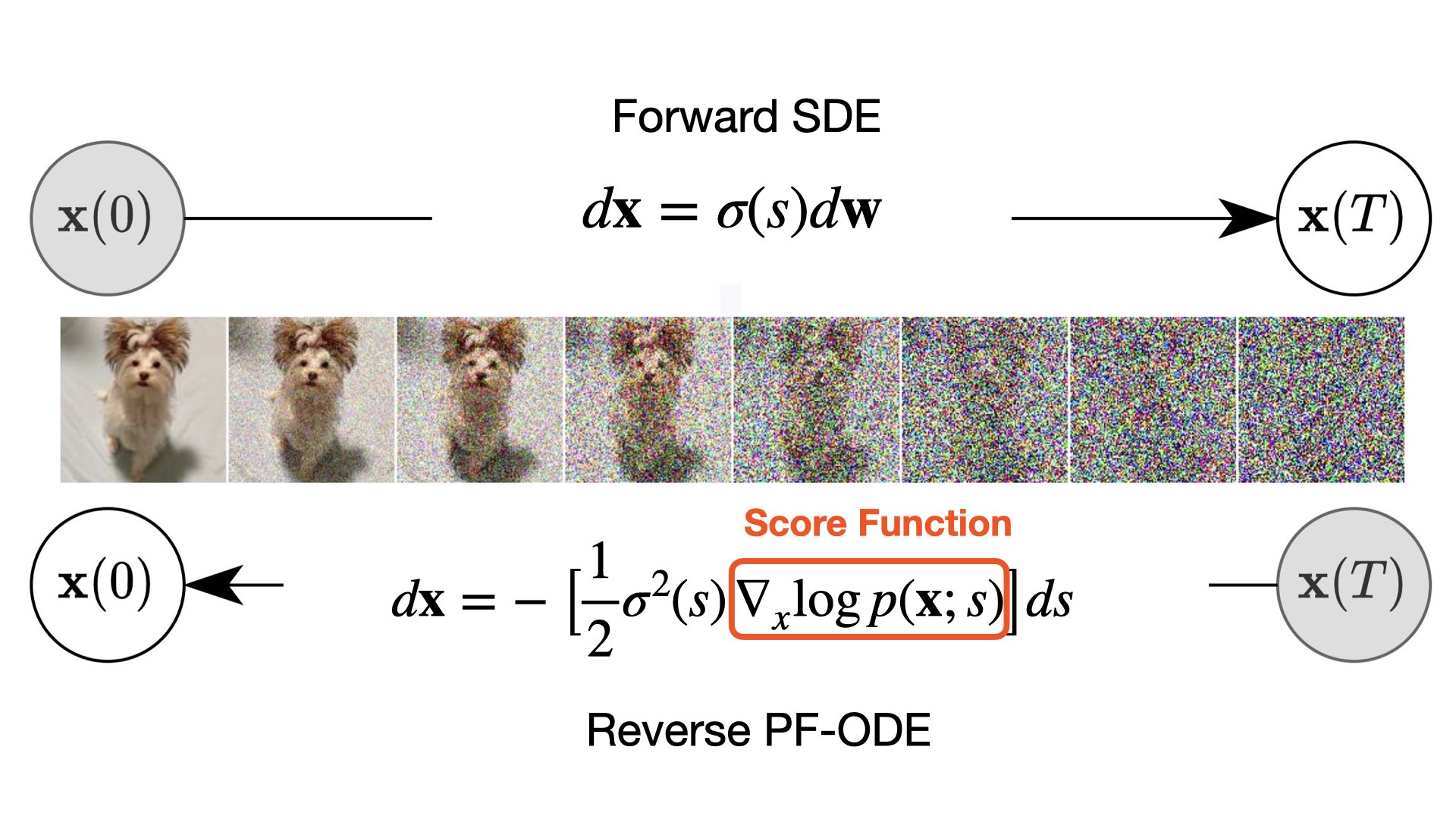
Figure 2: Diffusion Models through the lens of PF-ODEs, adapted from [2]. The forward (corrupting) process takes a true data point at time $s=0$ and corrupts the data into pure noise at time $s=T$ using an SDE. The reverse (reconstructing) process undoes the corruption using the score of the distribution. Both equations are shown without drift terms as in Eq. 7 and Eq. 8.

where $\alpha(t)\in R$ is a step size in the direction $F_{\bm{\theta}}$. Note that Eq. 3 is described using the convention that time progresses forward when reconstructing the data. However, the literature around DMs describes time in the reconstruction process as going backwards, denoting $x^{T}$ to refer to the sample drawn from pure noise and $x^{0}$ to refer to the final reconstructed sample drawn from $p$ [1, 2, 4, 19, 21]. Eq. 4 rewrites Eq. 3 using the variable $s\triangleq T-t$ to represent the reverse-time convention used in most DM papers (shown in Figure 2).

$$\mathbf{x}^{s-1}=\mathbf{x}^{s}+\alpha\mathbf{F}_{\bm{\theta}}(\mathbf{x}^{s}),\;\;\;\;\;\;s=T,...,1$$ (4)

Using score-based models is then conceptually very simple: they seek to maximize (minimize) the log-likelihood (energy) of an initial sample by following the score $\mathbf{F}_{\bm{\theta}}$ (energy gradient). In practice, many of the functions above are additionally conditioned on the time $s$; i.e., the p.d.f. can be expressed as $p_{\bm{\theta}}(\mathbf{x};s)$, the score function can be expressed as $\mathbf{F}_{\bm{\theta}}(\mathbf{x};s)$, and the step size $\alpha$ can be expressed as $\alpha(s)$. We are also free to condition the score function however we desire; e.g., controllable image generation using DMs express the tokens $\mathbf{C}$ of language prompts as a conditioning variable on the score function $\mathbf{F}_{\bm{\theta}}(\mathbf{x};t,\mathbf{C})$ [8, 10, 52].

3.2 Diffusion Models Cleverly Train the Score

Though simple in concept, DMs require several tricks to train. How do you train the “score” of a dataset? Several techniques to train the score-based models have been proposed, with the most popular being the technique of denoising score-matching [53, 2, 54, 55, 56, 4]. To train with denoising score-matching, samples $\mathbf{x}$ from our original data distribution $p$ are repeatedly perturbed with small amounts of noise $\boldsymbol{\eta}(s)$. We then train our score-based model $\mathbf{F}_{\bm{\theta}}(\mathbf{x}^{s+1})$ to remove the noise added at the previous step. If the added noise is small enough, we can guarantee that our optimal score function (parameterized by optimal weights $\bm{\theta}^{*}$) approximates the score of the true data distribution: i.e., $\mathbf{F}_{{\bm{\theta}}^{*}}(\mathbf{x})\approx\nabla_{\mathbf{x}}\log p(\mathbf{x})$ and $\mathbf{F}_{{\bm{\theta}}^{*}}(\mathbf{x}^{s+1})\approx-\boldsymbol{\eta}(s)$. This process of noisifying a signal is known as the forward process, which we also call the corruption process.

The original DM proposed by [1] trained their model using a forward process consisting of $T=1000$ noise-adding steps. Unfortunately, to sample from DMs each step in the forward process must be paired with a step in the reconstruction or reverse process, which likewise required $T=1000$ steps/applications of the score network $\mathbf{F}_{\bm{\theta}}(\mathbf{x}^{s})$. [2] improved the computational efficiency by introducing several techniques into the forward process, including a form of annealed Langevin dynamics where larger noises are added the further you are from the original data distribution, controlled by a variance scheduler $\sigma(s)\in\mathbb{R}$. They then introduce Noise Conditional Score Networks (NCSNs) to condition the score network $\mathbf{F}_{\bm{\theta}}(\mathbf{x};\sigma(s))$ on the amount of noise $\sigma(s)$ to remove. Because the $\sigma(s)$ has a 1:1 correspondence to a particular time step $s$, NCSNs can also be written as $\mathbf{F}_{\bm{\theta}}(\mathbf{x};s)$.

3.3 Diffusion Models are Continuous Neural ODEs

The original DM [1] and NCSN [2] relied on a fixed number of discrete steps in the forward and reverse process and could not work without Langevin dynamics (stochastic descent down the energy function during reconstruction). [21] introduced a probability flow Ordinary Differential Equation (PF-ODE) formulation for DMs to unify and extend previous approaches, which [34, 57, 58] claim represents the culmination of DM theory for several reasons.

1. PF-ODEs show that Langevin dynamics are optional to making DMs work, a phenomena also detected by [59]. Deterministic forward and reverse processes perform just as well as those formulated stochastically.

2. PF-ODEs operate in continuous time and do not require a fixed number of discrete time-steps or noise scales. This makes it possible to use black-box ODE solvers during the reverse-process enabling faster generation than previously possible.

3. PF-ODEs enable exact log-likelihood calculations, drawing connections to normalizing flows [47, 48] and neural ODEs [60]. This perspective proffers DMs as a new technique to solve inverse problems.

4. The latent encodings for each step of PF-ODEs are both meaningful and uniquely identifiable. Given a sufficiently performant model trained on sufficient data, we can interfere with latent representations to perform tasks the model was not originally trained to perform (e.g., inpainting, outpainting, interpolation, temperature scaling, etc.)

The importance of PF-ODEs to the modern understanding of DMs cannot be overstated and warrants sufficient background. Consider the standard form of a generic ODE under constrained time $s$:

$$\frac{d\mathbf{x}}{ds}=\boldsymbol{\mu}(\mathbf{x};s),\;\;\;\;\;\;s\in[T,0]$$ (5)

where $\boldsymbol{\mu}(\mathbf{x};s)$ is an arbitrary drift function that represents some deterministic change in position of particle $\mathbf{x}^{s}$ at time $s$. Diffusion models need to further corrupt the input $\mathbf{x}$, so we add to Eq. 5 an infinitesimal amount of noise $\frac{d\mathbf{w}}{ds}$ scaled by some real-valued diffusion coefficient $\sigma(s)$. The forward process of PF-ODEs is now called an Itô Stochastic Differential Equation (SDE) [21].

$$\frac{d\mathbf{x}}{ds}=\boldsymbol{\mu}(\mathbf{x};s)+\sigma(s)\frac{d\mathbf{w}}{ds}$$ (6)

[58] argues that the equation above can be further simplified without any loss in performance by assuming a constant drift function $\boldsymbol{\mu}(\mathbf{x};s)=0$, a convention adapted by [57] to set SOTA one-step generation with DMs. This convention simplifies Eq. 6 to make the forward process depend only on a noise scale and the infinitesimal random noise shown in Eq. 7.

$$\frac{d\mathbf{x}}{ds}=\sigma(s)\frac{d\mathbf{w}}{ds}.$$ (7)

The reverse process now depends only on the noise scale $\sigma$ and the score $\mathbf{F}_{\bm{\theta}}$ [21, 57]

$$\frac{d\mathbf{x}}{ds}=-\frac{1}{2}\sigma^{2}(s)\mathbf{F}_{\bm{\theta}}(\mathbf{x};s)\,.$$ (8)

We have written the strange “reverse time” convention of DMs using time variable $s\triangleq T-t$. Eq. 9 rewrites Eq. 8 using forward time $t$ and collects the noise scale into a real-valued time-variable $\tau(t)\triangleq\frac{2}{\sigma^{2}(t)}$ to control the rate of change.

$$\tau(t)\frac{d\mathbf{x}}{dt}=\mathbf{F}_{\bm{\theta}}(\mathbf{x};t)\,,\;\;\;\;\;\;t\in[0,T]$$ (9)

PF-ODEs unify previous theories of DMs by simplifying the assumptions needed to make DMs work. At the same time, the continuous dynamics of PF-ODEs exposes a strong mathematical connection to Associative Memories that was difficult to see before.

4 Associative Memories

An Associative Memory (AM) is a dynamical system concerned with the storage and retrieval of signals (data). In AMs all signals exist on an energy landscape; in general, the more corrupted a signal the higher its energy value. Uncorrupted signals or memories live at local minima of the system’s energy or Lyapunov function. The process of memory retrieval is the dynamic process of descending the energy to a fixed point or memory as shown in Figure 1, a phenomenon that is guaranteed to occur by constraints placed on the architecture (see § 4.1).

The following subsections describing AMs can get quite technical and rely on modeling techniques used regularly in physics (e.g., Lagrangian functions, Lyapunov functions, Legendre transforms [18, 61]) but that are foreign to experts in modern AI. We thus deem it important to summarize the core points of AMs before diving into them and their history.

AMs are a class of neural architectures that defines an energy function $E_{\bm{\theta}}(\mathbf{x})\in\mathbb{R}$, where ${\bm{\theta}}$ is a set of learnable parameters and $\mathbf{x}$ represents a data point. In other words, an AM is designed to compute a scalar energy on every possible input signal $\mathbf{x}$. Given some initial input $\mathbf{x}^{0}$ at time $t=0$ (this could be any kind of signal, including pure noise), we want to minimize the energy (by descending the gradient) to a fixed point that represents a memory learned from the original data distribution.

$$\tau\frac{d\mathbf{x}}{dt}=-\nabla_{\mathbf{x}}E_{\bm{\theta}}(\mathbf{x})\,,\;\;\;\;\;\;t>0$$ (10)

Here, $\tau$ is a time constant that governs how quickly the dynamics evolve. This equation can of course be discretized as

$$\mathbf{x}^{t+1}=\mathbf{x}^{t}-\frac{dt}{\tau}\nabla_{\mathbf{x}}E_{\bm{\theta}}(\mathbf{x}^{t})$$ (11)

and treated as a neural network that is recurrent through time. The energy of AMs is constructed in such a way that the dynamics will eventually converge to a fixed point $\mathbf{x}^{\star}$ at some $t=T$. That is,

$$\frac{d\mathbf{x}^{\star}}{dt} =0\hskip 11.38092pt\mathrm{and}$$

$$\mathbf{x}^{\star} =\mathbf{x}^{\star}-\frac{dt}{\tau}\nabla_{\mathbf{x}}E_{\bm{\theta}}(\mathbf{x}^{\star})\,\;\;\;\;\;\;\forall t>T\,.$$

4.1 The TinyBrain Sandbox for Building Associative Memories

AMs are constrained to use only neural architectures that are themselves a Lyapunov function: that is, these architectures must compute a scalar energy and be fixed point attractors. In this section we discuss the architectural constraints needed to ensure a Lyapunov function on AMs, following the abstractions of [62].

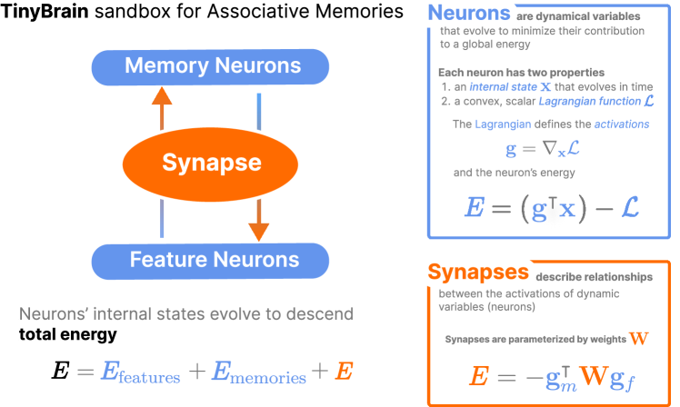
Figure 3: The TinyBrain sandbox for understanding Associative Memories is a fully connected bipartite graph (structurally similar to the Restricted Boltzmann Machine [63]). Both feature neurons and memory neurons have states $\mathbf{x}_{f}$ and $\mathbf{x}_{m}$ respectively that evolve in time; these states have corresponding activations $\mathbf{g}_{f}$ and $\mathbf{g}_{m}$. The energy of the synapse is minimized when the memory activations $\mathbf{g}_{m}$ perfectly align with the feature activations $\mathbf{g}_{f}$ according to the learned parameters $\mathbf{W}$. The energy for the entire system is defined by this the energies of each individual component, and the internal states of each neuron layer evolve by descending the global energy’s gradient.

AMs were originally inspired by neurons and synapses within the brain [64]. As such, it is useful to consider a simple model we call the TinyBrain model as depicted in Figure 3. The TinyBrain model consists of two dynamic variables called neuron layers connected to each other by a single synaptic weight matrix $\mathbf{W}$ (relationship between variables). Each neuron layer (dynamic variable) can be described by an internal state $\mathbf{x}\in\mathbb{R}^{N}$ (which one can think of as the membrane voltage for each of the $N$ neurons in that layer), and their axonal state $\mathbf{g}\in\mathbb{R}^{N}$ (which is analogous to the firing rate of each neuron). We call the axonal state the activations and they are uniquely constrained to be the gradient of a scalar, convex Lagrangian function $\mathcal{L}:\mathbb{R}^{N}\mapsto\mathbb{R}$ we choose for that layer; that is, $\mathbf{g}=\nabla_{\mathbf{x}}\mathcal{L}$.

The Legendre Transform of the Lagrangian defines the energy $E^{\mathrm{layer}}_{\nu}(\mathbf{g}_{\nu},\mathbf{x}_{\nu})\in\mathbb{R}$ of a neuron layer $\nu$, shown in Eq. 12 [18, 61, 62]. If all neuron-layers of a system have a Lagrangian, a synaptic energy can be easily found such that the entire system has a defined energy.

$$E^{\mathrm{layer}}_{\nu}=\mathbf{g}_{\nu}^{\intercal}\mathbf{x}_{\nu}-\mathcal{L}_{\nu}(\mathbf{x}_{\nu})$$ (12)

For historical reasons, we call one neuron layer in our TinyBrain the “feature neurons” (fully described by the internal state $\mathbf{x}_{f}$ and Lagrangian $\mathcal{L}_{f}$ of the features) and the other the “memory neurons” (fully described by the internal state $\mathbf{x}_{m}$ and Lagrangian $\mathcal{L}_{m}$ of the memories). These layers are connected to each other via a synaptic weight matrix $\mathbf{W}\in\mathbb{R}^{N_{m}\times N_{f}}$, creating a synaptic energy $E^{\mathrm{synapse}}(\mathbf{g}_{f},\mathbf{g}_{m};\mathbf{W})\in\mathbb{R}$ defined as

$$E^{\mathrm{synapse}}=-\mathbf{g}_{m}^{\intercal}\mathbf{W}\mathbf{g}_{f}\,.$$ (13)

We now have defined all the component energies necessary to write the total energy $E^{\mathrm{system}}$ for TinyBrain as in Eq. 14. Note that Eq. 14 is a simple summation of the energies of each component of the TinyBrain: two layer energies and one synaptic energy. This perspective of modular energies for understanding AMs was originally proposed by [62].

$$E^{\mathrm{system}}=E^{\mathrm{layer}}_{f}+E^{\mathrm{layer}}_{m}+E^{\mathrm{synapse}}$$ (14)

The hidden states of our neurons $\mathbf{x}_{f}$ and $\mathbf{x}_{m}$ evolve in time according to the general update rule:

$$\begin{dcases}\tau_{f}\frac{d\mathbf{x}_{f}}{dt}&=-\nabla_{\mathbf{g}_{f}}E^{\mathrm{system}}\vspace{0.1cm}\\ \tau_{m}\frac{d\mathbf{x}_{m}}{dt}&=-\nabla_{\mathbf{g}_{m}}E^{\mathrm{system}}\,.\end{dcases}$$ (15)

Eq. 15 reduces to the manually derived update equations for the feature and memory layers presented in Eq. 16 [18].

$$\begin{dcases}\tau_{f}\frac{d\mathbf{x}_{f}}{dt}&=\mathbf{W}^{\intercal}\mathbf{g}_{m}-\mathbf{x}_{f}\vspace{0.1cm}\\ \tau_{m}\frac{d\mathbf{x}_{m}}{dt}&=\mathbf{W}\mathbf{g}_{f}-\mathbf{x}_{m}\end{dcases}$$ (16)

where $\mathbf{W}^{\intercal}\mathbf{g}_{m}$ and $\mathbf{W}\mathbf{g}_{f}$ represent the input currents to feature neurons and memory neurons respectively, and $-\mathbf{x}_{f}$ and $-\mathbf{x}_{m}$ represent exponential decay (this implies that the internal state $\mathbf{x}$ will exponentially decay to $\mathbf{0}$ in the absence of input current). Note that the synaptic matrix $\mathbf{W}$ plays a symmetric role: the same weights that modulate the current from feature neurons $\rightarrow$ memory neurons are used to modulate the current from memory neurons $\rightarrow$ feature neurons. This “symmetric weight constraint” present in AMs does not exist in real neurons and synapses [18, 65].

Krotov and Hopfield identified [18] that this toy model is mathematically equivalent to the original Hopfield Network [64, 66] under certain choices of the activation function $\mathbf{g}$; hence, it is through the lens of the abstraction presented in this section that we explore the long history of AMs, beginning with the famous Hopfield Network.

4.2 Hopfield Networks are the First Energy-Based Associative Memory

John Hopfield formalized the dynamic retrieval process of Associative Memory in the 80s [64, 66] in an energy-based model that became famously known as the Hopfield Network (HN). Unlike previous models for associative memory (see § 4.5), HNs performed the task of memory retrieval through gradient descent of an energy function. A HN resembles in form a single-layer McCulloch & Pitts perceptron [67], with input feature neurons $\mathbf{x}_{f}$ and a single weight matrix; however, unlike perceptron-based models, the HN operated continuously in time, repeatedly updating the inputs $\mathbf{x}_{f}^{t}$ over time to minimize some energy.

Hopfield described the AM energy dynamics for both binary [64] and graded (continuous) [66] neurons. Like the TinyBrain model, a continuous HN consists of $N_{f}$ feature neurons connected via a synaptic weight matrix $\mathbf{W}\in\mathbb{R}^{N_{m}\times N_{f}}$ to $N_{m}$ memory neurons. Feature neurons $\mathbf{x}_{f}$ have corresponding activations $\mathbf{g}_{f}=\operatorname{sigmoid}(\mathbf{x}_{f})$, whereas memory neurons $\mathbf{x}_{m}$ have a linear activation function $\mathbf{g}_{m}=\mathbf{x}_{m}$. We call this configuration of TinyBrain the Classical Hopfield Network (CHN).

Hopfield never considered the time evolution of the memory neurons in his model, instead assuming that $\mathbf{x}_{m}^{t}=W\mathbf{g}_{f}^{t}$ at any point in time (i.e., that the state of the memory neurons was instantaneously defined by the activations of the feature neurons). This simplification of the two-layer TinyBrain did not change the fixed points of the AM dynamics and allowed him to consider the time-evolution for only the feature neuron layer. The simplified energy function and update rules for the CHN are shown in Eq. 17 and Eq. 18 respectively, where $\mathcal{L}_{f}(\mathbf{x}_{f})\triangleq\sum_{N_{f}}\log\left(1+\exp(\mathbf{x}_{f})\right)$ is the Lagrangian of the $\operatorname{sigmoid}$ activation function and $(\cdot)^{2}$ operates elementwise.

$$E^{\mathrm{system}}(\mathbf{g}_{f},\mathbf{x}_{f}) =-\frac{1}{2}\sum\limits_{N_{m}}\big{(}\mathbf{W}\mathbf{g}_{f}\big{)}^{2}+\mathbf{g}_{f}^{\intercal}\mathbf{x}_{f}-\mathcal{L}_{f}(\mathbf{x}_{f})$$ (17)

$$\tau\frac{d\mathbf{x}_{f}}{dt} =\mathbf{W}^{\intercal}(\mathbf{W}\mathbf{g}_{f})-\mathbf{x}_{f}\,.$$ (18)

A full derivation is included in [18].

4.3 Solving the Small Memory Capacity of Hopfield Networks

The CHN unfortunately suffered from a tiny memory capacity that scaled linearly according the number of input features $N_{f}$; specifically, the maximum storage capacity of the classical Hopfield Network was discovered to be ${\sim}0.14N_{f}$ by [68, 64, 69]. Consider the problem of building an associative memory on the $60$k images in MNIST [70], where each image can be represented as a binary vector with $N_{f}=784$ features. If the patterns were random, one could only reliably store a maximum of $0.14(784)\approx 110$ images using the classical Hopfield paradigm, no matter how many memories $N_{m}$ you add to the synaptic matrix $\mathbf{W}$. Given that MNIST images have strong correlations between their pixel intensities, this bound is even lower.

A breakthrough in the capacity of Hopfield Networks was proposed by Krotov & Hopfield over 30 years later [67]. Their new network, called the Dense Associative Memory (DAM), enabled the energy dynamics of the CHN to store a super-linear number of memories. The core idea was to use a rapidly growing non-linear activation functions $\mathbf{g}_{m}(\cdot)$ on the memory neurons. For instance, choosing $\mathbf{g}_{m}(\cdot)$ to be higher orders of (optionally rectified) polynomials allowed much greater memory storage capacity than the CHN. Extending this idea to exponential functions $\mathbf{g}_{m}=\exp(\mathbf{x}_{m})$ can even lead to exponential storage capacity [71]. The intuition is that the “spikier” the activation function $\mathbf{g}_{m}$ (i.e., the faster it grows in the region around $\mathbf{x}_{m}$), the more memories the network can store and retrieve.

Recall that a CHN could reliably store a maximum of $110$ MNIST images. Using the exponential DAM, one can increase the number of stored memories up to $N_{m}\sim\exp(784/2)$, assuming no correlations, and still reliably retrieve each individual memory. This marked difference has led to DAMs being branded as the “Modern Hopfield Network” (MHN) [31] and opened the door for a new frontier in AMs [43].

4.4 Adding Hierarchy to Shallow Associative Memories

The CHN and DAM have another fundamental limitation: like the TinyBrain, both only have a single weight matrix $\mathbf{W}$ and thus cannot learn hierarchical abstractions that simplify the task of memorizing complex signals. This is not a limitation of Deep Learning networks today, which can be seen as a stack of distinct learnable functions (“layers”) each processing the output of a previous layer. These architectures are inherently hierarchical; that is, deeper layers operate on higher levels of abstraction output by previous layers. A classic example of this occurs in deep Convolutional Neural Networks (CNNs), where neurons in earlier layers (i.e., layers closer to the image) detect simple shapes, and those in deeper layers respond to more complex objects (see Figure 4).

However, Eq. 12 makes it easy to constrain the energy of an AM. Why can’t these systems be extended beyond the TinyBrain in § 4.1 to include more interacting layers? This is the realization of [61, 62] who generalize the theoretical abstraction of AMs in § 4.1 to connect arbitrary numbers of neuron layers via arbitrary synaptic relationships that can resemble the convolutional, pooling, or even attention operations in modern architectures. This version of AMs is known as a Hierarchical Associative Memory (HAM).

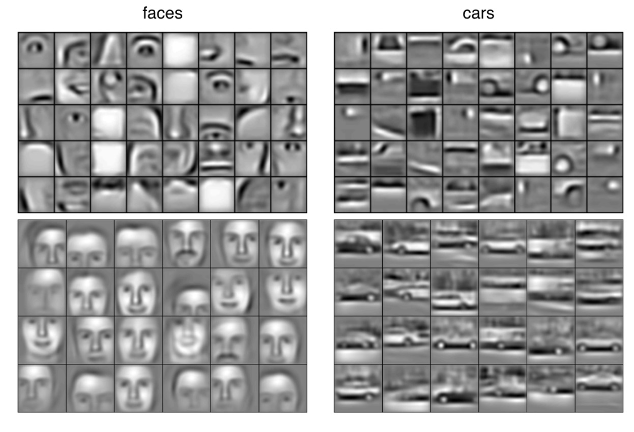
Figure 4: An explanation of hierarchical representations as learned in images, adapted from [72]. The top row shows the filters learned by the second layer in a convolutional deep belief network, whereas the bottom row the filters of the third layer. The deeper filters are able to recognize more complex objects and are thus considered more “abstract”.

The HAM has given AMs a theoretical maturity and flexibility to rival the representational capacity of any existing neural architecture while guaranteeing stable attractor points. However, the HAM is still a very young architecture, having been proposed in 2021, and has yet to establish itself as a viable alternative to traditional Deep Learning architectures in practice.

4.5 Other models for Associative Memory

The term “associative memory” has become a catch-all term for many different types of Content Addressable Memories (CAMs), including models like Sparse Distributed Memories [73, 74],Memory Networks [75], Key-Value Memories [76, 77], Hopfield Networks [64, 66], and Boltzmann Machines [78, 79, 63]. Even the popular attention mechanism in Transformers [30] is itself a differentiable form of associative memory [31] where tokens act as queries to retrieve values stored by the other tokens. In this paper we have considered a particular class of AMs that refers to systems with a defined Lyapunov function – that is, a CAM must have both a tractable energy function and guaranteed stable states to be considered in this survey. The paradigmatic examples of this class of AMs is of course the Hopfield Network (HN) [64, 66] and its modern counterparts [67, 61] which have been discussed in earlier sections.

Table 1: Summarizing the similarities and differences between Diffusion Models and Associative Memory. Fields marked with a ^∗ indicate caveats. See § 5.1 and § 5.2 for details.

	Diffusion	Associative Memory
Parameterizes the$\ldots$	Score function $\mathbf{F}_{\bm{\theta}}$	Energy function $E_{\bm{\theta}}$
Continuous Update	$\tau\frac{d\mathbf{x}}{dt}=\mathbf{F}_{\bm{\theta}}(\mathbf{x})$	$\tau\frac{d\mathbf{x}}{dt}=-\nabla_{\mathbf{x}}E_{\bm{\theta}}(\mathbf{x})$
Discrete Update	$\mathbf{x}^{t+1}=\mathbf{x}^{t}+\alpha\mathbf{F}_{\bm{\theta}}(\mathbf{x}^{t})$	$\mathbf{x}^{t+1}=\mathbf{x}^{t}-\alpha\nabla_{\mathbf{x}}E_{\bm{\theta}}(\mathbf{x}^{t})$
Valid Time Domain	$t\in[0,T]$	$t\geq 0$
Fixed Point Attractor?	No∗	Yes
Tractable Energy?	No∗	Yes
Undoes Corruption of $\ldots$	Noise it was trained on∗	Any kind

5 An Uncanny Resemblance between Associative Memories and Diffusion Models

Associative Memories are different from Diffusion Models in that they are not primarily understood as generative models. This said, the memory retrieval process can be easily be construed as a “generation process” that samples from some original distribution. This process can be visualized as follows. We first pick a point at random on our energy landscape by initializing a data point $\mathbf{x}^{0}$ to random noise. We then descend the energy (as in Eq. 10) until the system settles in the nearest local minimum $\mathbf{x}^{\star}$: this retrieved memory is our generated sample. If desired, small amounts of noise can be added to each update step (a process called Langevin dynamics) that can help improve the diversity of generations and jar the dynamics out of undesirable local minima (a technique that is used regularly during generation in DMs [57, 3, 4, 1]). This realization makes it possible to directly compare AMs to DMs.

We tabulate the similarities and differences between DMs and AMs in Table 1, providing additional details in § 5.2.

5.1 Characterizing the Similarities

There are several reasons to be skeptical of significant overlap between generative models like DMs and AMs. As presented, DMs only compute gradients of energies and not energies themselves; thus they have no Lyapunov function guaranteeing stability and cannot operate continuously in time. However, it is clear that both DMs and AMs have very similar goals as shown in Eq. 9 and Eq. 10. We summarize the similarities between these two data modeling approaches as follows:

• Both model the energy. DMs learn a parameterized score function $\mathbf{F}_{\bm{\theta}}$ to approximate the gradient of some true energy function $E$ at every point $\mathbf{x}$ in the energy landscape such that $\mathbf{F}_{\bm{\theta}}(\mathbf{x})\approx-\nabla_{\mathbf{x}}E(\mathbf{x})$. In AMs, this energy function is explicit and is defined by using architectures that directly model the energy $E_{\bm{\theta}}$ such that $E_{\bm{\theta}}(\mathbf{x})\approx E(\mathbf{x})$.

• Both generate samples by descending the predicted gradient of the energy. A DM will directly output the estimated score $\mathbf{F}_{\bm{\theta}}\approx-\nabla_{\mathbf{x}}E(\mathbf{x})$, whereas an AM will directly output a smooth energy $E_{\bm{\theta}}(\mathbf{x})$ on which the gradient $-\nabla_{\mathbf{x}}E_{\bm{\theta}}(\mathbf{x})$ can be directly calculated and descended. The discrete (continuous) update rules of both are identical to a step size $\alpha$ (time variable $\tau$).

• Both converge to a solution that lies in the neighborhood of a local energy minimum. In DMs, this behavior is a consequence of the manner in which it is trained: the final output $\mathbf{x}^{T}$ exists in a region such that a small perturbation in any direction would increase its energy. In AMs, this statement is a requirement of the Lyapunov function; if the dynamics progress for a sufficiently long time, we are guaranteed to reach a true fixed point $\mathbf{x}^{\star}$ that lies at a local energy minimum.

5.2 Reconciling the Differences

DMs and AMs are certainly not equivalent methods. However, we have discovered evidence that the theoretical differences between DMs and AMs are not so significant in practice. We present rebuttals to potential objections (which we call “misconceptions”) that Diffusion Models do not simulate Associative Memories below.

Misconception 1: Diffusion models are not fixed point attractors.

Though the dynamics of DMs have no theoretical guarantees of fixed point attractors, we notice that the design of DMs seems to intelligently engineer the behavior of fixed-point attractors like AMs without constraining the architecture to represent a Lyapunov function. We identify two fundamental tricks used by DMs that help approximate stable dynamics:

Trick 1

DMs explicitly halt their reconstruction process at time $t=T$ (i.e., requiring $\mathbf{x}^{\star}=\mathbf{x}^{T}$) and are thus only defined for time $t\in[0,T]$. $\mathbf{x}^{T}$ then represents a contrived fixed point because no further operations change it. We can say that $\mathbf{x}^{t\neq T}$ corresponds to a data point with some corruption and $\mathbf{x}^{T}$ corresponds to a memory in the language of AMs.

Trick 2

We know that $\mathbf{x}^{T}$ approximates a local energy minimum because of the noise annealing trick introduced by [2] and used by all subsequent DMs. In the corruption process, points in the data distribution are perturbed with gradually increasing amounts of noise, implying that smaller noise is added at earlier points in time. This leads to a robust approximation of the true energy gradient localized around each training point, where the original data point lies at the minimum.

We additionally see evidence of DMs storing “memories” that are actual training points. [80] showed that one can retrieve training data almost exactly from publicly available DMs by descending an energy conditioned on prompts from the training dataset. It seems that this behavior is particularly evident for images considered outliers and for images that appear many times. Viewing DMs as AMs, this behavior is not surprising, as the whole function of AMs is to retrieve data (or close approximations to the data) that it has been seen before.

Tricks 1 & 2 also mean that a DM is inescapably bound to a knowledge of the current time $t$. The time $t$ defines not only how much noise the model should expect to remove from a given signal in a single step, but also how much total noise it should expect to remove from a given signal. Given a signal with an unknown quantity of noise, a user must either make a “best guess” for the time $t$ corresponding to this amount of noise, or restart the dynamics at time $t=0$ which will cause the model to make large jumps around the energy landscape and likely land it in a different energy minimum. Currently, AMs have no such dependence between corruption levels and time $t$ and can run continuously in time.

Misconception 2: Diffusion models can only undo Gaussian noise.

In order for a DM to behave like an AM, they must be able to undo any kind of corruption (e.g., inpainting, blur, pixelation, etc.), not just the white- or Gaussian-noise associated with Brownian motion as originally formulated in [1, 2]. [81, 82] showed that the performance of DMs can actually improve when considering other types of noisy corruption in the forward process. However, it also seems that DMs can learn to reverse any kind of corrupting process. [59] empirically show that DMs can be trained to invert arbitrary image corruptions that generate samples just as well as those trained to invert Gaussian noise. Because DMs can be trained to undo any kind of corruption, they can exhibit behavior identical to that of Associative Memory which focuses on the “fixed points” of the energy landscape rather than the kind of denoising/de-corrupting steps required to get there.

Misconception 3: Unconstrained Diffusion Models work with any architecture.

One advantage of DMs over AMs is that they are “unconstrained” and can use any neural network architecture to approximate the score function; in other words, the architecture is not required to be the gradient of an actual scalar energy. The only requirement is that the neural network chosen to approximate the score must be isomorphic such that the function’s output is the same shape as its input (i.e., $\mathbf{F}_{\bm{\theta}}:\mathbb{R}^{d}\mapsto\mathbb{R}^{d}$). However, not all isomorphic architectures are created equal and only select architectures are used in practice. Both standard feedforward networks [51] and vanilla Transformers have struggled to generate quality samples using diffusion [83, 84]. Most applications of DMs use some modification of the U-Net architecture [85] originally used by [4], though the original DM paper [1] used shallow MLPs, and recent work [83] has shown how to engineer vision Transformers [86] to achieve a similar reconstruction quality as U-Nets on images.

Misconception 4: Diffusion Models with explicit energy don’t work.

Though DMs characterize an energy landscape by modeling its gradient everywhere, they do not inherently have a concept of the energy value itself. However, [21] showed that one can actually compute an exact energy for DMs using the instantaneous change of variables formula from [87], with the caveat that this equation is expensive to compute; estimations over direct calculations of the energy computation are preferred in practice [20].

Another approach for enforcing an energy on DMs is to choose an architecture that parameterizes an actual energy function, whose gradient is the score function. Ref. [51] researched exactly this, exploring whether a generic learnable function $\mathbf{f}_{\bm{\theta}}(\mathbf{x};t)$ that is constrained to be the true gradient of a parameterized energy function as in Eq. 19 is able to attain sample quality results similar to those of unconstrained networks.

$$E_{\bm{\theta}}(\mathbf{x};t)=\frac{1}{2\sigma(t)}||\mathbf{x}-\mathbf{f}_{\bm{\theta}}(\mathbf{x};t)||^{2}$$ (19)

The score $\mathbf{F}_{\bm{\theta}}$ of this energy can be written by computing the analytical gradient

$$\mathbf{F}_{\bm{\theta}}(\mathbf{x};t)=\frac{1}{\sigma(t)}(\mathbf{x}-\mathbf{f}_{\bm{\theta}}(\mathbf{x};t))\nabla_{\mathbf{x}}\mathbf{f}_{\bm{\theta}}(\mathbf{x};t)-\frac{1}{\sigma(t)}(\mathbf{x}-\mathbf{f}_{\bm{\theta}}(\mathbf{x};t))\,.$$ (20)

Ref. [51] notes that the second term of the equation is the standard DM, while the first term involving $\nabla_{\mathbf{x}}\mathbf{f}_{\bm{\theta}}(\mathbf{x};t)$ is new and helps guarantee that $\mathbf{F}_{\bm{\theta}}(\mathbf{x};t)$ is a conservative vector field. They also showed that constraining the score function to be the gradient of the energy in Eq. 19 does not hurt the generation performance on the CIFAR dataset [88] and provides hope that AMs with constrained energy can match the performance of unconstrained DMs.

6 Conclusions & Open Challenges

Diffusion Models and Associative Memories have remarkable similarities when presented using a unified mathematical notation: both aim to minimize some energy (maximize some log-probability) by following its gradient (score). The final solution of both approaches represents some sort of memory that lies in a local minimum (maximum) of the energy (log-probability). However, these approaches are certainly not identical, as is evidenced by different validity constraints on architecture choices and time domains. The training philosophy behind each approach is also different: Diffusion Models assume that the energy function is intractable and fixate on training the gradient of the energy (using known perturbations of training data as the objective), while AMs focus on learning the fixed points of a tractable energy.

6.1 Directions for Associative Memories

Associative Memories have not gained nearly the traction of Diffusion Models in AI applications. Many researchers in the field focus on the TinyBrain architecture, trying to improve its theoretical memory capacity [89, 90] or apply related models to modern problems [91]. Other researchers are integrating the memory-retrieval capabilities of AMs into existing feed-forward architectures [31, 92, 93]; in doing so they discard the idea of global optimization on the energy. In part, these other research directions exist because no pure AM has shown impressive performance on large data until [32] introduced the Energy Transformer, though even this AM does not yet show significant performance gain over traditional methods.

The empirical success of Diffusion Models across many domains should provide hope that modern AM architectures [61, 62] can achieve performance parity on similar tasks. Constrained Diffusion Models show no worse performance than unconstrained models [51], and the introduction of HAMs allow AMs to be built that resemble U-Nets [62]. Even the training pipeline of a Diffusion Model can be mapped directly to an AM paradigm if we condition the energy function and optimization procedure on the time: from a starting image $\mathbf{x}^{\star}$ in the training set, repeatedly add varying amounts of random noise and train the score function $-\nabla_{\mathbf{x}}E_{\theta}(\mathbf{x}^{t};t)$ to predict the added noise. Once trained, Diffusion Models have even shown strong steerability – the ability for a user to modify a trained Diffusion Model to complete tasks it was not trained to perform [1, 94, 95, 96, 52, 97, 98, 99, 100]. We can expect similar levels of controllability from a fully trained AM.

6.2 Directions for Diffusion Models

Diffusion Models should find the theoretical framework of the Lyapunov function from AMs compelling, as it defines systems around fixed-point attractors that seem to already exist in Diffusion Models. Perhaps the score function $\mathbf{F}_{\theta}$ learned by Diffusion Models has already learned to behave similarly? If the score function is shown to be a conservative vector field as in [51], perhaps the constraint of finite time in Diffusion Models is unnecessary and Diffusion Models can behave well in continuous time $t>T$. Viewing Diffusion Models as fundamentally fixed-point attractors like AMs, it also becomes possible to theoretically characterize its memory capacity. Finally, recent research has focused on optimizing the sampling speed of Diffusion Models by improving the scheduling step in the update rule [57, 101, 102, 103]. By viewing this sampling procedure as ordinary gradient descent (as is the case in AMs), smart gradient optimization techniques already used in Deep Learning like ADAM [104] and L-BFGS [105] become available.

6.3 Beyond Diffusion: Transformers Resemble Associative Memories

Diffusion Models are not the only method in modern Deep Learning to show similarities to AMs. In fact, recent literature shows increasing connections between the operations of AMs and deep architectures, e.g. feed-forward networks [93], convolutional neural networks [61], Transformer architecture [31], and optimization processes of Ordinary Differential Equations (ODEs) [106, 107, 108, 109]. In 2020 [31] discovered that the attention mechanism of Transformers strongly resembled a single-step update of a Dense Associative Memory [67] under the $\operatorname{softmax}(\cdot)$ activation function, which exhibits similar properties to the power and $\exp(\cdot)$ functions studied in [67, 71]. However, it is incorrect to call their contrived energy function an AM as it is integrated as a conventional feed-forward layer in the standard Transformer block and applied only using a single gradient descent step. Of particular interest to the scope of this paper is the following question: if Transformers have strong resemblances to ODEs and the attention operation is similar to a single step update of a DAM, what are the differences between an AM with desirable attractor dynamics and a Transformer?

A recent work by [32] explores this question, deriving a new “Energy Transformer” block that strongly resembles the conventional Transformer block, but whose fundamental operation outputs an energy. This energy satisfies all the desired properties of an AM, which allows us to interpret the forward pass through a stack of Transformer blocks as gradient descent down the block’s energy.

6.4 Scaling Laws from the Perspective of Associative Memory

The performance of Transformers on language is famously characterized by the “scaling laws”, which claim that a model’s performance will improve as a power-law with model size, dataset size, and the amount of compute used for training [110]. We expect similar behaviors to hold for Diffusion Models, though a similar study has not yet been conducted. However, the “scaling laws” are empirical only, and there is little theory to justify why a model’s performance would continue to grow with the size. AMs offer one possible theory by characterizing large-model performance as one of memory capacity (see § 4.3). In the world of AMs, this scaling behavior makes intuitive sense: more parameters means more possible memories that can be stored; more data means more meaningful local minima in the energy; and more compute means the model can descend further down the energy, making it easier to distinguish between nearby fixed points (alternatively, more compute can imply that longer training allows the model to distribute the fixed points in the energy more efficiently, allowing for greater memory capacity). These hypotheses for understanding the scaling law come from intuitively understanding large models as AMs, but this is still an open research question.

Both Transformers and Diffusion Models are ubiquitous choices for foundation models [111] in Deep Learning today, and both strongly resemble Associative Memories. We believe that the trajectory of AI research would benefit by interpreting the problem of unsupervised learning on large, unstructured data from the perspective of Associative Memory.

6.5 Closing Remarks

Very few researchers will observe the rapid advances of AI today and notice a trend towards the dynamical processes of Associative Memories first established by John Hopfield in the 1980s. However, many of the theoretical guarantees of Associative Memories are captured in the design of increasingly popular Diffusion Models that have proven themselves fixtures for many applications of generative modeling. This survey represents a first step towards a more comprehensive understanding of the connections between Diffusion Models and Associative Memories. We hope that our work inspires further research into these exciting fields and that it helps to foster a new generation of AI systems that are capable of unlocking the secrets of memory and perception.

Appendix A Mathematical Notations

All mathematical notation used in this paper is documented in Table 2. When applicable, we describe the notation both by its data-science (e.g., “data point”) and physics terminology (e.g., “particle”).

Table 2: A summary of the mathematical notations and conventions used in this survey.

Notation	Description
$t$	time
$s$	reverse time (as $s$ increases, time $t$ decreases. Used in diffusion literature)
${\bm{\theta}}$	parameters for neural network
$p_{\bm{\theta}}$	probability distribution of some data, parameterized by ${\bm{\theta}}$
$E_{\bm{\theta}}$	energy of some data, parameterized by ${\bm{\theta}}$, proportional to the negative of log-probability
$Z_{\bm{\theta}}$	normalization constant converting energy to probabilities a.k.a. the partition function
$\mathbf{F}_{\bm{\theta}}$	score function or the force (equal to $-\nabla_{\mathbf{x}}E_{\bm{\theta}}$), parameterized by ${\bm{\theta}}$
$\alpha$	discrete step size when descending the energy
$\eta$	noise added during discrete forward-process of diffusion
$d\mathbf{w}$	infinitesimal noise added during continuous forward process of diffusion
$\sigma(s)$	noise scale of $d\mathbf{w}$ added at time $s$ of continuous forward-process in diffusion
$T$	max depth of a Diffusion Model / time that fixed point of AM is reached
$\tau$	rate constant of continuous time dynamics
$N_{\nu}$	number of neurons in layer $\nu$ of AMs
$\mathbf{x}$	state of a data point, evolves in time (position of particle)
$\mathbf{g}$	activations of state $\mathbf{x}$ (axonal output of a neuron)
$\mathcal{L}$	Lagrangian of a layer (dynamic variable) that defines that variable’s energy and activations
$\mathbf{x}^{\star}$	fixed point of the memory retrieval dynamics
$\mathbf{W}$	weights of the Associative Memory network
$\mathbf{f}_{\theta}$	any generic function parameterized by $\bm{\theta}$
$\boldsymbol{\mu}(\mathbf{x})$	drift term in diffusion’s corruption process, typically set to $\mathbf{0}$

References

- [1] Jascha Sohl-Dickstein, Eric A. Weiss, Niru Maheswaranathan, and Surya Ganguli. Deep Unsupervised Learning using Nonequilibrium Thermodynamics, November 2015.
- [2] Yang Song and Stefano Ermon. Generative Modeling by Estimating Gradients of the Data Distribution. In Advances in Neural Information Processing Systems, volume 32. Curran Associates, Inc., 2019.
- [3] Yang Song and Stefano Ermon. Improved Techniques for Training Score-Based Generative Models. In Advances in Neural Information Processing Systems, volume 33, pages 12438–12448. Curran Associates, Inc., 2020.
- [4] Jonathan Ho, Ajay Jain, and Pieter Abbeel. Denoising Diffusion Probabilistic Models. In Advances in Neural Information Processing Systems, volume 33, pages 6840–6851. Curran Associates, Inc., 2020.
- [5] Prafulla Dhariwal and Alexander Quinn Nichol. Diffusion Models Beat GANs on Image Synthesis. In Advances in Neural Information Processing Systems, November 2021.
- [6] Aditya Ramesh, Prafulla Dhariwal, Alex Nichol, Casey Chu, and Mark Chen. Hierarchical Text-Conditional Image Generation with CLIP Latents, April 2022.
- [7] Chitwan Saharia, William Chan, Saurabh Saxena, Lala Li, Jay Whang, Emily Denton, Seyed Kamyar Seyed Ghasemipour, Raphael Gontijo-Lopes, Burcu Karagol Ayan, Tim Salimans, Jonathan Ho, David J. Fleet, and Mohammad Norouzi. Photorealistic Text-to-Image Diffusion Models with Deep Language Understanding. In Advances in Neural Information Processing Systems, May 2022.
- [8] Robin Rombach, Andreas Blattmann, Dominik Lorenz, Patrick Esser, and Björn Ommer. High-resolution image synthesis with latent diffusion models. In Proceedings of the IEEE/CVF Conference on Computer Vision and Pattern Recognition, pages 10684–10695, 2022.
- [9] Alex Nichol, Prafulla Dhariwal, Aditya Ramesh, Pranav Shyam, Pamela Mishkin, Bob McGrew, Ilya Sutskever, and Mark Chen. GLIDE: Towards Photorealistic Image Generation and Editing with Text-Guided Diffusion Models, March 2022.
- [10] Midjourney, 2023.
- [11] Jonathan Ho, Tim Salimans, Alexey A. Gritsenko, William Chan, Mohammad Norouzi, and David J. Fleet. Video Diffusion Models. In Advances in Neural Information Processing Systems, May 2022.
- [12] Gabriele Corso, Hannes Stärk, Bowen Jing, Regina Barzilay, and Tommi S. Jaakkola. DiffDock: Diffusion Steps, Twists, and Turns for Molecular Docking. In The Eleventh International Conference on Learning Representations, September 2022.
- [13] Zhifeng Kong, Wei Ping, Jiaji Huang, Kexin Zhao, and Bryan Catanzaro. DiffWave: A Versatile Diffusion Model for Audio Synthesis. In International Conference on Learning Representations, October 2020.
- [14] Nanxin Chen, Yu Zhang, Heiga Zen, Ron J. Weiss, Mohammad Norouzi, and William Chan. WaveGrad: Estimating Gradients for Waveform Generation. In International Conference on Learning Representations, October 2020.
- [15] Vadim Popov, Ivan Vovk, Vladimir Gogoryan, Tasnima Sadekova, and Mikhail Kudinov. Grad-tts: A diffusion probabilistic model for text-to-speech. In International Conference on Machine Learning, pages 8599–8608. PMLR, 2021.
- [16] Peiyu Yu, Sirui Xie, Xiaojian Ma, Baoxiong Jia, Bo Pang, Ruiqi Gao, Yixin Zhu, Song-Chun Zhu, and Ying Nian Wu. Latent diffusion energy-based model for interpretable text modeling. In Proceedings of International Conference on Machine Learning (ICML), July 2022.
- [17] William James. The Principles of Psychology, Vol I. The Principles of Psychology, Vol I. Henry Holt and Co, New York, NY, US, 1890.
- [18] Dmitry Krotov and John J. Hopfield. Large associative memory problem in neurobiology and machine learning. In International Conference on Learning Representations, 2021.
- [19] David McAllester. On the Mathematics of Diffusion Models, February 2023.
- [20] Will Grathwohl, Ricky T. Q. Chen, Jesse Bettencourt, Ilya Sutskever, and David Duvenaud. FFJORD: Free-Form Continuous Dynamics for Scalable Reversible Generative Models. In International Conference on Learning Representations, September 2018.
- [21] Yang Song, Jascha Sohl-Dickstein, Diederik P. Kingma, Abhishek Kumar, Stefano Ermon, and Ben Poole. Score-Based Generative Modeling through Stochastic Differential Equations. In International Conference on Learning Representations, October 2020.
- [22] Phillip Lippe. Tutorial 7: Deep Energy-Based Generative Models, September 2021.
- [23] Yu Takagi and Shinji Nishimoto. High-resolution image reconstruction with latent diffusion models from human brain activity. In Proceedings of the IEEE/CVF Conference on Computer Vision and Pattern Recognition, pages 14453–14463, 2023.
- [24] James C. R. Whittington, Joseph Warren, and Tim E.J. Behrens. Relating transformers to models and neural representations of the hippocampal formation. In International Conference on Learning Representations, 2022.
- [25] Jiakun Fu, Suhas Shrinivasan, Kayla Ponder, Taliah Muhammad, Zhuokun Ding, Eric Wang, Zhiwei Ding, Dat T. Tran, Paul G. Fahey, Stelios Papadopoulos, Saumil Patel, Jacob Reimer, Alexander S. Ecker, Xaq Pitkow, Ralf M. Haefner, Fabian H. Sinz, Katrin Franke, and Andreas S. Tolias. Pattern completion and disruption characterize contextual modulation in mouse visual cortex, March 2023.
- [26] Furkan Ozcelik and Rufin VanRullen. Brain-Diffuser: Natural scene reconstruction from fMRI signals using generative latent diffusion, March 2023.
- [27] Aria Y. Wang, Kendrick Kay, Thomas Naselaris, Michael J. Tarr, and Leila Wehbe. Incorporating natural language into vision models improves prediction and understanding of higher visual cortex, September 2022.
- [28] Arjun Majumdar, Karmesh Yadav, Sergio Arnaud, Yecheng Jason Ma, Claire Chen, Sneha Silwal, Aryan Jain, Vincent-Pierre Berges, Pieter Abbeel, Dhruv Batra, Yixin Lin, Oleksandr Maksymets, Aravind Rajeswaran, and Franziska Meier. Where are we in the search for an Artificial Visual Cortex for Embodied Intelligence? In Workshop on Reincarnating Reinforcement Learning at ICLR 2023, March 2023.
- [29] Leo Kozachkov, Ksenia V Kastanenka, and Dmitry Krotov. Building transformers from neurons and astrocytes. Proceedings of the National Academy of Sciences, 120(34):e2219150120, 2023.
- [30] Ashish Vaswani, Noam Shazeer, Niki Parmar, Jakob Uszkoreit, Llion Jones, Aidan N Gomez, Łukasz Kaiser, and Illia Polosukhin. Attention is all you need. In I. Guyon, U. Von Luxburg, S. Bengio, H. Wallach, R. Fergus, S. Vishwanathan, and R. Garnett, editors, Advances in Neural Information Processing Systems, volume 30. Curran Associates, Inc., 2017.
- [31] Hubert Ramsauer, Bernhard Schäfl, Johannes Lehner, Philipp Seidl, Michael Widrich, Lukas Gruber, Markus Holzleitner, Thomas Adler, David Kreil, Michael K. Kopp, Günter Klambauer, Johannes Brandstetter, and Sepp Hochreiter. Hopfield Networks is All You Need. In International Conference on Learning Representations, February 2022.
- [32] Benjamin Hoover, Yuchen Liang, Bao Pham, Rameswar Panda, Hendrik Strobelt, Duen Horng Chau, Mohammed J. Zaki, and Dmitry Krotov. Energy Transformer, February 2023.
- [33] Ling Yang, Zhilong Zhang, Yang Song, Shenda Hong, Runsheng Xu, Yue Zhao, Yingxia Shao, Wentao Zhang, Bin Cui, and Ming-Hsuan Yang. Diffusion Models: A Comprehensive Survey of Methods and Applications, October 2022.
- [34] Eric J. Ma. A Pedagogical Introduction to Score Models, April 2022.
- [35] Calvin Luo. Understanding Diffusion Models: A Unified Perspective, August 2022.
- [36] Karsten Kreis, Ruiqi Gao, and Arash Vahdat. Denoising Diffusion-based Generative Modeling: Foundations and Applications.
- [37] James Thorton and De Bortoli. What’s the score? – Review of latest Score Based Generative Modeling papers., 2023.
- [38] Humayun Karim Sulehria and Ye Zhang. Hopfield neural networks: A survey. In Proceedings of the 6th Conference on 6th WSEAS Int. Conf. on Artificial Intelligence, Knowledge Engineering and Data Bases, volume 6, pages 125–130. Citeseer, 2007.
- [39] A. G. Hanlon. Content-Addressable and Associative Memory Systems a Survey. IEEE Transactions on Electronic Computers, EC-15(4):509–521, August 1966.
- [40] B. D. C. N. Prasad, P. E. S. N. Krishna Prasad, Sagar Yeruva, and P. Sita Rama Murty. A Study on Associative Neural Memories. International Journal of Advanced Computer Science and Applications (IJACSA), 1(6), February 2012.
- [41] V. I. Gritsenko, D. A. Rachkovskij, A. A. Frolov, R. Gayler, D. Kleyko, and E. Osipov. Neural Distributed Autoassociative Memories: A Survey. Kibern. vyčisl. teh., 2017(2(188)):5–35, June 2017.
- [42] T. Poggio. From Associative Memories to Deep Networks. 2021.
- [43] Dmitry Krotov. A new frontier for hopfield networks. Nature Reviews Physics, pages 1–2, 2023.
- [44] Diederik P. Kingma and Max Welling. Auto-Encoding Variational Bayes. December 2013.
- [45] Danilo Jimenez Rezende, Shakir Mohamed, and Daan Wierstra. Stochastic Backpropagation and Approximate Inference in Deep Generative Models. In Proceedings of the 31st International Conference on Machine Learning, pages 1278–1286. PMLR, June 2014.
- [46] Angus Turner. Diffusion Models as a kind of VAE, June 2021.
- [47] Laurent Dinh, David Krueger, and Yoshua Bengio. NICE: Non-linear Independent Components Estimation, April 2015.
- [48] Laurent Dinh, Jascha Sohl-Dickstein, and Samy Bengio. Density estimation using Real NVP. In International Conference on Learning Representations, November 2016.
- [49] Wenbo Gong and Yingzhen Li. Interpreting diffusion score matching using normalizing flow. In ICML Workshop on Invertible Neural Networks, Normalizing Flows, and Explicit Likelihood Models, June 2021.
- [50] Roland S. Zimmermann, Lukas Schott, Yang Song, Benjamin Adric Dunn, and David A. Klindt. Score-Based Generative Classifiers. In NeurIPS 2021 Workshop on Deep Generative Models and Downstream Applications, December 2021.
- [51] Tim Salimans and Jonathan Ho. Should EBMs model the energy or the score? In Energy Based Models Workshop - ICLR 2021, April 2021.
- [52] Lvmin Zhang, Anyi Rao, and Maneesh Agrawala. Adding conditional control to text-to-image diffusion models, 2023.
- [53] Yang Song, Sahaj Garg, Jiaxin Shi, and Stefano Ermon. Sliced score matching: A scalable approach to density and score estimation. In Uncertainty in Artificial Intelligence, pages 574–584. PMLR, 2020.
- [54] Aapo Hyvärinen and Peter Dayan. Estimation of non-normalized statistical models by score matching. Journal of Machine Learning Research, 6(4), 2005.
- [55] Martin Raphan and Eero Simoncelli. Least Squares Estimation Without Priors or Supervision. Neural computation, 23:374–420, February 2011.
- [56] Pascal Vincent. A Connection Between Score Matching and Denoising Autoencoders. Neural Computation, 23(7):1661–1674, July 2011.
- [57] Yang Song, Prafulla Dhariwal, Mark Chen, and Ilya Sutskever. Consistency Models. In International Conference for Machine Learning, January 2023.
- [58] Tero Karras, Miika Aittala, Timo Aila, and Samuli Laine. Elucidating the Design Space of Diffusion-Based Generative Models. In Advances in Neural Information Processing Systems, May 2022.
- [59] Arpit Bansal, Eitan Borgnia, Hong-Min Chu, Jie S. Li, Hamid Kazemi, Furong Huang, Micah Goldblum, Jonas Geiping, and Tom Goldstein. Cold Diffusion: Inverting Arbitrary Image Transforms Without Noise, August 2022.
- [60] Patrick Kidger. On Neural Differential Equations, February 2022.
- [61] Dmitry Krotov. Hierarchical Associative Memory, July 2021.
- [62] Benjamin Hoover, Duen Horng Chau, Hendrik Strobelt, and Dmitry Krotov. A Universal Abstraction for Hierarchical Hopfield Networks. In The Symbiosis of Deep Learning and Differential Equations II, October 2022.
- [63] Geoffrey E. Hinton. Training Products of Experts by Minimizing Contrastive Divergence. Neural Computation, 14(8):1771–1800, August 2002.
- [64] J J Hopfield. Neural networks and physical systems with emergent collective computational abilities. Proceedings of the National Academy of Sciences, 79(8):2554–2558, April 1982.
- [65] David J. C. MacKay and David J. C. Mac Kay. Information Theory, Inference and Learning Algorithms. Cambridge University Press, September 2003.
- [66] John Hopfield. Neurons With Graded Response Have Collective Computational Properties Like Those of Two-State Neurons. Proceedings of the National Academy of Sciences of the United States of America, 81:3088–92, June 1984.
- [67] Dmitry Krotov and John J. Hopfield. Dense associative memory for pattern recognition. In D. Lee, M. Sugiyama, U. Luxburg, I. Guyon, and R. Garnett, editors, Advances in Neural Information Processing Systems, volume 29. Curran Associates, Inc., 2016.
- [68] Y. Abu-Mostafa and J. St. Jacques. Information capacity of the Hopfield model. IEEE Transactions on Information Theory, 31(4):461–464, July 1985.
- [69] Daniel J Amit, Hanoch Gutfreund, and Haim Sompolinsky. Storing infinite numbers of patterns in a spin-glass model of neural networks. Physical Review Letters, 55(14):1530, 1985.
- [70] Li Deng. The mnist database of handwritten digit images for machine learning research. IEEE Signal Processing Magazine, 29(6):141–142, 2012.
- [71] Mete Demircigil, Judith Heusel, Matthias Löwe, Sven Upgang, and Franck Vermet. On a Model of Associative Memory with Huge Storage Capacity. J Stat Phys, 168(2):288–299, July 2017.
- [72] Honglak Lee, Roger Grosse, Rajesh Ranganath, and Andrew Y. Ng. Convolutional deep belief networks for scalable unsupervised learning of hierarchical representations. In Proceedings of the 26th Annual International Conference on Machine Learning, pages 609–616, Montreal Quebec Canada, June 2009. ACM.
- [73] Louis A. Jaeckel. An alternative design for a sparse distributed memory. July 1989.
- [74] Pentti Kanerva. Sparse Distributed Memory. MIT press, 1988.
- [75] Jason Weston, Sumit Chopra, and Antoine Bordes. Memory Networks, November 2015.
- [76] Danil Tyulmankov, Ching Fang, Annapurna Vadaparty, and Guangyu Robert Yang. Biological learning in key-value memory networks. Advances in Neural Information Processing Systems, 34:22247–22258, 2021.
- [77] Alexander Miller, Adam Fisch, Jesse Dodge, Amir-Hossein Karimi, Antoine Bordes, and Jason Weston. Key-Value Memory Networks for Directly Reading Documents, October 2016.
- [78] Geoffrey E Hinton, Terrence J Sejnowski, and David H Ackley. Boltzmann Machines: Constraint Satisfaction Networks That Learn. Carnegie-Mellon University, Department of Computer Science Pittsburgh, PA, 1984.
- [79] David H Ackley, Geoffrey E Hinton, and Terrence J Sejnowski. A learning algorithm for Boltzmann machines. Cognitive science, 9(1):147–169, 1985.
- [80] Nicolas Carlini, Jamie Hayes, Milad Nasr, Matthew Jagielski, Vikash Sehwag, Florian Tramer, Borja Balle, Daphne Ippolito, and Eric Wallace. Extracting training data from diffusion models. In 32nd USENIX Security Symposium (USENIX Security 23), pages 5253–5270, 2023.
- [81] Vikram Voleti, Christopher Pal, and Adam Oberman. Score-based Denoising Diffusion with Non-Isotropic Gaussian Noise Models, November 2022.
- [82] Eliya Nachmani, Robin San Roman, and Lior Wolf. Non Gaussian Denoising Diffusion Models, June 2021.
- [83] Fan Bao, Chongxuan Li, Yue Cao, and Jun Zhu. All are Worth Words: A ViT Backbone for Score-based Diffusion Models. In NeurIPS 2022 Workshop on Score-Based Methods, November 2022.
- [84] Xiulong Yang, Sheng-Min Shih, Yinlin Fu, Xiaoting Zhao, and Shihao Ji. Your ViT is Secretly a Hybrid Discriminative-Generative Diffusion Model, August 2022.
- [85] Olaf Ronneberger, Philipp Fischer, and Thomas Brox. U-Net: Convolutional Networks for Biomedical Image Segmentation. In Nassir Navab, Joachim Hornegger, William M. Wells, and Alejandro F. Frangi, editors, Medical Image Computing and Computer-Assisted Intervention – MICCAI 2015, Lecture Notes in Computer Science, pages 234–241, Cham, 2015. Springer International Publishing.
- [86] Alexey Dosovitskiy, Lucas Beyer, Alexander Kolesnikov, Dirk Weissenborn, Xiaohua Zhai, Thomas Unterthiner, Mostafa Dehghani, Matthias Minderer, Georg Heigold, Sylvain Gelly, Jakob Uszkoreit, and Neil Houlsby. An Image is Worth 16x16 Words: Transformers for Image Recognition at Scale. In International Conference on Learning Representations, October 2020.
- [87] Ricky TQ Chen, Yulia Rubanova, Jesse Bettencourt, and David K Duvenaud. Neural ordinary differential equations. Advances in neural information processing systems, 31, 2018.
- [88] Alex Krizhevsky, Vinod Nair, and Geoffrey Hinton. CIFAR-10 (Canadian Institute for Advanced Research).
- [89] Beren Millidge, Tommaso Salvatori, Yuhang Song, Thomas Lukasiewicz, and Rafal Bogacz. Universal Hopfield Networks: A General Framework for Single-Shot Associative Memory Models. Proc Mach Learn Res, 162:15561–15583, July 2022.
- [90] Thomas F Burns and Tomoki Fukai. Simplicial hopfield networks. In The Eleventh International Conference on Learning Representations, 2023.
- [91] Yuchen Liang, Chaitanya K. Ryali, Benjamin Hoover, Leopold Grinberg, Saket Navlakha, Mohammed J. Zaki, and Dmitry Krotov. Can a Fruit Fly Learn Word Embeddings?, March 2021.
- [92] Michael Widrich, Bernhard Schäfl, Milena Pavlović, Hubert Ramsauer, Lukas Gruber, Markus Holzleitner, Johannes Brandstetter, Geir Kjetil Sandve, Victor Greiff, Sepp Hochreiter, and Günter Klambauer. Modern Hopfield Networks and Attention for Immune Repertoire Classification. In Advances in Neural Information Processing Systems, volume 33, pages 18832–18845. Curran Associates, Inc., 2020.
- [93] Dmitry Krotov and John Hopfield. Dense associative memory is robust to adversarial inputs. Neural computation, 30(12):3151–3167, 2018.
- [94] Tim Brooks, Aleksander Holynski, and Alexei A Efros. Instructpix2pix: Learning to follow image editing instructions. In Proceedings of the IEEE/CVF Conference on Computer Vision and Pattern Recognition, pages 18392–18402, 2023.
- [95] Nataniel Ruiz, Yuanzhen Li, Varun Jampani, Yael Pritch, Michael Rubinstein, and Kfir Aberman. Dreambooth: Fine tuning text-to-image diffusion models for subject-driven generation. In Proceedings of the IEEE/CVF Conference on Computer Vision and Pattern Recognition, pages 22500–22510, 2023.
- [96] Rinon Gal, Yuval Alaluf, Yuval Atzmon, Or Patashnik, Amit H. Bermano, Gal Chechik, and Daniel Cohen-Or. An Image is Worth One Word: Personalizing Text-to-Image Generation using Textual Inversion, August 2022.
- [97] Gaurav Parmar, Krishna Kumar Singh, Richard Zhang, Yijun Li, Jingwan Lu, and Jun-Yan Zhu. Zero-shot image-to-image translation. In ACM SIGGRAPH 2023 Conference Proceedings, pages 1–11, 2023.
- [98] Hila Chefer, Yuval Alaluf, Yael Vinker, Lior Wolf, and Daniel Cohen-Or. Attend-and-excite: Attention-based semantic guidance for text-to-image diffusion models. ACM Transactions on Graphics (TOG), 42(4):1–10, 2023.
- [99] Omer Bar-Tal, Lior Yariv, Yaron Lipman, and Tali Dekel. MultiDiffusion: Fusing Diffusion Paths for Controlled Image Generation, February 2023.
- [100] Manuel Brack, Felix Friedrich, Dominik Hintersdorf, Lukas Struppek, Patrick Schramowski, and Kristian Kersting. SEGA: Instructing Diffusion using Semantic Dimensions, January 2023.
- [101] Jiaming Song, Chenlin Meng, and Stefano Ermon. Denoising Diffusion Implicit Models, October 2022.
- [102] Tim Salimans and Jonathan Ho. Progressive Distillation for Fast Sampling of Diffusion Models. In International Conference on Learning Representations, October 2021.
- [103] Hongkai Zheng, Weili Nie, Arash Vahdat, Kamyar Azizzadenesheli, and Anima Anandkumar. Fast Sampling of Diffusion Models via Operator Learning. In NeurIPS 2022 Workshop on Score-Based Methods, November 2022.
- [104] Diederik P. Kingma and Jimmy Ba. Adam: A Method for Stochastic Optimization, January 2017.
- [105] Dong C. Liu and Jorge Nocedal. On the limited memory BFGS method for large scale optimization. Mathematical Programming, 45(1-3):503–528, August 1989.
- [106] Yiping Lu, Aoxiao Zhong, Quanzheng Li, and Bin Dong. Beyond Finite Layer Neural Networks: Bridging Deep Architectures and Numerical Differential Equations, March 2020.
- [107] Subhabrata Dutta, Tanya Gautam, Soumen Chakrabarti, and Tanmoy Chakraborty. Redesigning the transformer architecture with insights from multi-particle dynamical systems. Advances in Neural Information Processing Systems, 34:5531–5544, 2021.
- [108] Bei Li, Quan Du, Tao Zhou, Yi Jing, Shuhan Zhou, Xin Zeng, Tong Xiao, Jingbo Zhu, Xuebo Liu, and Min Zhang. ODE transformer: An ordinary differential equation-inspired model for sequence generation. In Proceedings of the 60th Annual Meeting of the Association for Computational Linguistics (Volume 1: Long Papers), pages 8335–8351, 2022.
- [109] Yaofeng Desmond Zhong, Tongtao Zhang, Amit Chakraborty, and Biswadip Dey. A Neural ODE Interpretation of Transformer Layers. In The Symbiosis of Deep Learning and Differential Equations II, November 2022.
- [110] Jared Kaplan, Sam McCandlish, Tom Henighan, Tom B. Brown, Benjamin Chess, Rewon Child, Scott Gray, Alec Radford, Jeffrey Wu, and Dario Amodei. Scaling Laws for Neural Language Models, January 2020.
- [111] Rishi Bommasani, Drew A. Hudson, Ehsan Adeli, Russ Altman, Simran Arora, Sydney von Arx, Michael S. Bernstein, Jeannette Bohg, Antoine Bosselut, Emma Brunskill, Erik Brynjolfsson, Shyamal Buch, Dallas Card, Rodrigo Castellon, Niladri Chatterji, Annie Chen, Kathleen Creel, Jared Quincy Davis, Dora Demszky, Chris Donahue, Moussa Doumbouya, Esin Durmus, Stefano Ermon, John Etchemendy, Kawin Ethayarajh, Li Fei-Fei, Chelsea Finn, Trevor Gale, Lauren Gillespie, Karan Goel, Noah Goodman, Shelby Grossman, Neel Guha, Tatsunori Hashimoto, Peter Henderson, John Hewitt, Daniel E. Ho, Jenny Hong, Kyle Hsu, Jing Huang, Thomas Icard, Saahil Jain, Dan Jurafsky, Pratyusha Kalluri, Siddharth Karamcheti, Geoff Keeling, Fereshte Khani, Omar Khattab, Pang Wei Koh, Mark Krass, Ranjay Krishna, Rohith Kuditipudi, Ananya Kumar, Faisal Ladhak, Mina Lee, Tony Lee, Jure Leskovec, Isabelle Levent, Xiang Lisa Li, Xuechen Li, Tengyu Ma, Ali Malik, Christopher D. Manning, Suvir Mirchandani, Eric Mitchell, Zanele Munyikwa, Suraj Nair, Avanika Narayan, Deepak Narayanan, Ben Newman, Allen Nie, Juan Carlos Niebles, Hamed Nilforoshan, Julian Nyarko, Giray Ogut, Laurel Orr, Isabel Papadimitriou, Joon Sung Park, Chris Piech, Eva Portelance, Christopher Potts, Aditi Raghunathan, Rob Reich, Hongyu Ren, Frieda Rong, Yusuf Roohani, Camilo Ruiz, Jack Ryan, Christopher Ré, Dorsa Sadigh, Shiori Sagawa, Keshav Santhanam, Andy Shih, Krishnan Srinivasan, Alex Tamkin, Rohan Taori, Armin W. Thomas, Florian Tramèr, Rose E. Wang, William Wang, Bohan Wu, Jiajun Wu, Yuhuai Wu, Sang Michael Xie, Michihiro Yasunaga, Jiaxuan You, Matei Zaharia, Michael Zhang, Tianyi Zhang, Xikun Zhang, Yuhui Zhang, Lucia Zheng, Kaitlyn Zhou, and Percy Liang. On the Opportunities and Risks of Foundation Models, July 2022.