Discovering environments with XRM

Abstract

Successful out-of-distribution generalization requires environment annotations. Unfortunately, these are resource-intensive to obtain, and their relevance to model performance is limited by the expectations and perceptual biases of human annotators. Therefore, to enable robust AI systems across applications, we must develop algorithms to automatically discover environments inducing broad generalization. Current proposals, which divide examples based on their training error, suffer from one fundamental problem. These methods add hyper-parameters and early-stopping criteria that are impossible to tune without a validation set with human-annotated environments, the very information subject to discovery. In this paper, we propose Cross-Risk Minimization (XRM) to address this issue. XRM trains two twin networks, each learning from one random half of the training data, while imitating confident held-out mistakes made by its sibling. XRM provides a recipe for hyper-parameter tuning, does not require early-stopping, and can discover environments for all training and validation data. Domain generalization algorithms built on top of XRM environments achieve oracle worst-group-accuracy, solving a long-standing problem in out-of-distribution generalization.

1 Introduction

AI systems pervade our lives, spanning applications such as finance (Hand and Henley, 1997), healthcare (Jiang et al., 2017), self-driving vehicles (Bojarski et al., 2016), and justice (Angwin et al., 2016). While machines appear to outperform humans on such tasks, these systems fall apart when deployed in testing conditions different to their experienced training environments (Geirhos et al., 2020). For instance, during the COVID-19 pandemic, it was shown that thoracic x-ray classifiers latched onto spurious correlations—such as patient age, scanning position, or text fonts—as shortcuts to minimize their own training error (Heaven, 2021). This resulted in “an alarming situation in which the systems appear accurate, but fail when tested in new hospitals” (DeGrave et al., 2021).

Generally speaking, AI systems perform worse on groups of examples under-represented in the training data (Barocas et al., 2019). To drive this point home, consider the left side of figure 1, illustrating the Waterbirds problem (Sagawa et al., 2019). This task considers two class labels, landbirds and waterbirds, collected in two landscape environments, land and water. These combine into four groups: a majority group of waterbirds in water (73% of training examples), landbirds in land (22%), waterbirds in land (4%), and a minority group of landbirds in water (1%). On this problem, learning machines latch onto the landscape spurious feature, because it can separate the majority of examples, exhibits a larger signal-to-noise ratio, and yields the maximum-margin classifier amongst those with zero training error. For instance, consider an empirical risk minimization (Vapnik, 1998, ERM) baseline, which ignores environment information. As shown in the right panel of figure 1, ERM results in a worst-group-accuracy of $61\%{}$—attained, in fact, on the minority group.

To improve upon ERM, researchers have developed a myriad of domain generalization (DG) algorithms (Zhou et al., 2022; Wang et al., 2021). These methods consider environment annotations to uncover invariant (environment-generic) patterns and discard spurious (environment-specific) correlations (Arjovsky et al., 2019). As figure 1 shows, the DG algorithm group distributionally robust optimization (Sagawa et al., 2019, GroupDRO) achieves a worst-group-accuracy of $87\%{}$. This outperforms ERM by over twenty five points, a sizeable gap!

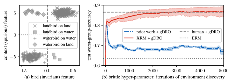
Figure 1: (a) Waterbirds classification problem, containing four groups: a majority group of waterbirds in water, landbirds in land, waterbirds in land, and a minority group of landbirds in water. Learning machines latch onto spurious landscape features, as it allows to classify the majority of examples, exhibits a larger signal-to-noise ratio, and yields the maximum-margin classifier amongst solutions with zero training error. (b) Worst-group-accuracy (minority-group-accuracy) for different methods. (Dotted line) An ERM baseline ignoring group annotations achieves $61\%{}$. (Dashed line) The GroupDRO domain generalization method with human group annotations, considered our oracle, achieves $87\%{}$. (Dashdot blue line) Prior work to discover groups requires early-stopping with surgical precision. This is an impossible ask without a validation set with human group annotations, the very information subject to discovery. Realistically, these methods would converge at $68\%{}$. (Solid red line) Our proposed XRM enables an oracle performance of $87\%{}$ at convergence.

While promising, DG algorithms require environment annotations. These are resource-intensive to obtain, and their relevance to downstream model performance is limited by the expectations, precision, and perceptual biases of human annotators. Moreover, no fixed environment annotations that we may choose and revise can serve the idiosyncrasies of all the different DG algorithms. In extremis, and by virtue of the combinatorial-explosion of ways in which two examples can be similar or dissimilar (Goodman, 1972), the patterns that deceive a learning system could be alien or invisible to our human eyes (Goodfellow et al., 2014). Because of these reasons, robust AI systems are currently confined to small data collections, and their promise in the large-scale setting remains unfulfilled.

In light of the above, some researchers began developing algorithms for the automatic discovery of environments from data (Bao and Barzilay, 2022; Zheran Liu et al., 2021; Lahoti et al., 2020; Dagaev et al., 2021; Creager et al., 2020; Nam et al., 2020). In broad strokes, these methods build a robust system in two phases. In phase-1, these methods learn a label predictor to distribute training examples in two environments, based on their training error. In phase-2, a DG algorithm is trained on top of the discovered environments to produce the robust system of interest. Unfortunately, this pipeline suffers from one fundamental issue. In particular, phase-1 needs to control the capacity of the label predictor with surgical precision, such that the discovered environments differ only in spurious correlation. As illustrated in figure 1, these methods discover environments that yield strong phase-2 systems only at the knife’s edge of very precisely early-stopped phase-1 training iterations—yielding a decent but still worse than oracle performance of $79\%{}$—and otherwise converge to a worst-group-accuracy of $68\%{}$. Unfortunately, we lack a signal for such a fine call, so methods for environment discovery resort to a validation set with human environment annotations. In practice, this wraps phase-1 and phase-2 with a cross-validation envelope to directly select a model maximizing validation worst-group-accuracy. Alas, at least in our view, this defeats the raison d’être of environment discovery.

Contribution

We propose Cross-Risk Minimization (XRM), a simple method for environment discovery that requires no human environment annotations whatsoever. XRM trains two twin label predictors, each holding-in one random half of the training data. During training, XRM instructs each twin to imitate confident held-out mistakes made by their sibling. This results in an “echo-chamber” where twins increasingly rely on bias, converging on a pair of environments that differ in spurious correlation, and share the invariances that fuel downstream out-of-distribution generalization. After twin training, a simple cross-mistake formula allows XRM to annotate all of the training and validation examples with environments. As our experiments show, XRM endows DG algorithms with oracle-like performance across benchmarks, solving a long-standing problem in out-of-distribution generalization. Returning one final time to figure 1, we observe that XRM+GroupDRO converges to $87\%{}$ worst-group-accuracy on Waterbirds, matching the oracle!

The sequel is as follows. Section 2 reviews the setup of DG, pointing-out the need for environment annotations as one of its major shortcomings. Section 3 surveys prior works on environment discovery, their issues surrounding hyper-parameter tuning and early-stopping, and their consequent reliance on validation sets with human environment annotations. Section 4 introduces XRM, a novel objective to discover machine-tailored environments for all training and validation data. Experiments in Section 5 show that DG algorithms built on top of XRM environments achieve oracle-like performance, and Section 6 closes with thoughts for future work.

2 Learning invariances across known environments

In domain generalization (DG), our goal is to build learning systems that perform well beyond the distribution of the training data. To this end, we collect examples under multiple training environments. Then, DG algorithms search for patterns that are invariant across these training environments—more likely to hold during test time—while discarding environment-specific spurious correlations (Arjovsky et al., 2019). More formally, we would like to learn a predictor $f$ to classify inputs $x$ into their appropriate labels $y$, and across all relevant environments $e\in\mathcal{E}$:

$$f\in\mathop{\mathrm{argmin}}_{\tilde{f}}\sup_{e\in\mathcal{E}}R^{e}(\tilde{f}),$$ (1)

where the risk $R^{e}(f)=\mathbb{E}_{(x,y)\sim P^{e}}[\ell(f(x),y)]$ measures the average loss $\ell$ incurred by the predictor $f$ across examples from environment $e$, all of them drawn iid from $P^{e}$.

In practical applications, the DG problem (1) is under-specified in two important ways. Firstly, we only get to train on a subset of all of the relevant environments $\mathcal{E}$, called the training environments $\mathcal{E}_{\text{tr}}\subset\mathcal{E}$. Yet, the quality of our predictor continues to be the worst classification accuracy across all environments $\mathcal{E}$. Secondly, and for each training environment $e\in\mathcal{E}_{\text{tr}}$, we do not observe its entire data distribution $P^{e}$, but only a finite set of iid examples $(x_{i},y_{i},e_{i}=e)$. In sum, the information at our disposal to address the DG problem (1) is the training dataset $\mathcal{D}_{\text{tr}}=\{(x_{i},y_{i},e_{i})\}_{i=1}^{n}$, where $(x_{i},y_{i})$ is an input-label pair drawn from the distribution $P^{e_{i}}$ associated to the training environment $e_{i}\in\mathcal{E}_{\text{tr}}$. Armed with $\mathcal{D}_{\text{tr}}$, we approximate (1) by the observable optimization problem

$$f\in\mathop{\mathrm{argmin}}_{\tilde{f}}\sup_{e\in\mathcal{E}_{\text{tr}}}R_{n}^{e}(\tilde{f}),$$ (2)

where $R^{e}_{n}(f)=\frac{1}{|\mathcal{D}^{e}_{\text{tr}}|}\sum_{(x_{i},y_{i})\in\mathcal{D}^{e}_{\text{tr}}}\ell(f(x_{i}),y_{i})$ is the empirical risk (Vapnik, 1998) across the data $\mathcal{D}^{e}_{\text{tr}}=\{(x_{i},y_{i})\in\mathcal{D}_{\text{tr}}:e_{i}=e\}$ from the training environment $e\in\mathcal{E}_{\text{tr}}$.

Environments and groups

In its full generality, domain generalization is an admittedly daunting task. To alleviate the burden, much prior literature considers the simplified version of group shift (Sagawa et al., 2019). The problem formulation is equivalent: we observe each input $x_{i}$ together with some attribute $e_{i}$ and label $y_{i}$, and define one group $g\equiv e\times y$ per attribute-label combination. (We use the terms “environment” and “attribute” interchangeably.) Again, we assume access to one training set of triplets $(x_{i},y_{i},e_{i})$ to learn our predictor, and one similarly formatted validation set available for hyper-parameter tuning and model selection purposes. Next, we put in place one important simplifying assumption $\mathcal{E}=\mathcal{E}_{\text{tr}}$, namely no new environments appear during test time. Consequently, the quality of our predictor can be directly estimated as the worst-group-accuracy in the validation set. Because most learning algorithms focus on minimizing average training error, oftentimes the worst-group-accuracy happens to be on the group with the smallest number of examples, also known as the minority group.

In practice, different DG algorithms (Gulrajani and Lopez-Paz, 2020; Zhou et al., 2022; Wang et al., 2021; Yang et al., 2023) target different types of invariance, learned across training environments $\mathcal{E}_{\text{tr}}$, assumed to hold across testing environments $\mathcal{E}_{\text{te}}$, and implemented as various innovations to the objective (2). As discussed in section 1, some DG algorithms outperform by a large margin methods ignoring environment (cf. attribute, group) information, such as ERM.

Despite their promise, the main roadblock towards large-scale domain generalization is their reliance on humanly annotated environments, attributes, or groups. These annotations are resource-intensive to obtain. Moreover, the expectations, precision, and perceptual biases of annotators can lead to environments conducive of sub-optimal out-of-distribution generalization. Different machine learning models fall prey to different kinds of spurious correlations. In addition, there are plenty of complex and subtle interactions between environment definition, function class, distributional shift, and cultural viewpoint (Lopez-Paz et al., 2022). Therefore, environment annotations are helpful only when revealing spurious and invariant patterns under the lens of the learning system under consideration. Could it be possible to design algorithms for the automatic discovery of environments tailored to the learning machine and data at hand?

3 Discovering environments

Nature does not shuffle data—Bottou (2019)

Let us reconsider the problem of domain generalization without access to environment annotations. This time it suffices to talk about one training distribution $P^{\text{tr}}$ and one testing distribution $P^{\text{te}}$. Our training data is a collection of input-label pairs $(x_{i},y_{i})$, each drawn iid from the training distribution. While the training distribution $P^{\text{tr}}$ may be the mixture of multiple environments describing interesting invariant and spurious correlations, this rich heterogeneity is shuffled together and unbeknown to us. But, if we could “unshuffle” the training distribution and recover the environments therein, we could invoke the domain generalization machinery from the previous section and hope for a robust predictor. This is the purpose of automatic environment discovery.

To discover environments and learn from them, most prior work implements a pipeline with two phases. On phase-1, train a label predictor and distribute each training example into two environments, depending on whether the example is correctly or incorrectly classified. On phase-2, train a DG algorithm on top of the discovered environments. Crucially, one must control the capacity of the label predictor in phase-1 with surgical precision, such that it relies only on prominent, easier-to-learn spurious correlations. If the environments discovered in phase-1 differ only in spurious correlation, as we would like, then the DG algorithm from phase-2 should be able to zero-in on invariant patterns more likely to generalize to the test distribution $P^{\text{te}}$. On the unlucky side, if phase-1 produces a zero-training-error predictor, we would be providing phase-2 with one non-vacuous, non-informative environment—the training data itself!

As a result, proposals for environment discovery differ mainly in how to control the capacity of the phase-1 label predictor. For example, the too-good-to-be-true prior (Dagaev et al., 2021) employs a predictor with a small parameter count. Just train twice (Zheran Liu et al., 2021, JTT) and environment inference for invariant learning (Creager et al., 2020, EIIL) train a phase-1 predictor for a limited number of epochs. Learning from failure (Nam et al., 2020, LfF) biases the predictor towards the use of “simple” features by applying a generalized version of the cross entropy loss. Other proposals, such as learning to split (Bao and Barzilay, 2022, LS) and adversarial re-weighted learning (Lahoti et al., 2020, ARL) complement capacity control with adversarial games.

However regularized, all of these methods suffer from one fundamental problem. More specifically, these phase-1 strategies add hyper-parameters and early-stopping criteria, but remain silent on how to tune them. As illustrated in figure 1 for Waterbirds, methods like the above discover environments leading to competitive generalization only when phase-1 is trained for a number of iterations that fall within a knife’s edge. Quickly after that, the performance of the resulting phase-2 system falls off a cliff, landing at ERM-like worst-group-accuracy.

Prior works keep away from this predicament by assuming a validation set with human environment annotations. Then, it becomes possible to simply wrap phase-1 and phase-2 into a cross-validation pipeline that promotes validation worst-group-accuracy. Alas, this defeats the entire purpose of environment discovery. In fact, if we have access to a small dataset with human environment annotations, these examples suffice to fine-tune the last layer of a deep neural network towards state-of-the-art worst-group-accuracy (Izmailov et al., 2022). Looking forward, could we develop an algorithm for environment discovery that requires no human annotations whatsoever, and robustly yields oracle-like phase-2 performance?

4 Cross-Risk Minimization (XRM)

We propose Cross-Risk Minimization (XRM), an algorithm to discover environments without the need of human supervision. XRM comes with batteries included, namely a recipe for hyper-parameter tuning and a formula to annotate all training and validation data. As we will show in section 5, environments discovered by XRM endow phase-2 DG algorithms with oracle performance.

The blueprint for phase-1 with XRM is as follows. XRM trains two twin label predictors, each holding-in one random half of the training data (section 4.1). During training, XRM biases each twin to absorb spurious correlation by imitating confident held-out mistakes from their sibling (section 4.2). XRM chooses hyper-parameters for the twins based on the number of imitated mistakes (section 4.3). Finally, and given the selected twins, XRM employs a simple “cross-mistake” formula to discover environment annotations for all of the training and validation examples (section 4.4). Algorithm 1 serves as a companion to the descriptions below; appendix D contains a real PyTorch implementation. The runtime of phase-1 with XRM is akin to one ERM baseline on the training data.

Algorithm 1 Cross-Risk Minimization (XRM)

Input: training examples $\{(x_{i},y_{i})\}_{i=1}^{n}$ and validation examples $\{(\tilde{x}_{i},\tilde{y}_{i})\}_{i=1}^{m}$
Output: discovered environments for training $\{e_{i}\}_{i=1}^{n}$ and validation $\{\tilde{e}_{i}\}_{i=1}^{m}$ examples

• Fix held-in training example assignments $m^{a}_{i}\sim\text{Bernoulli}(\frac{1}{2})$ and $m^{b}_{i}=1-m^{a}_{i}$

• Init two label predictors $f^{a}$ and $f^{b}$ at random; calibrate softmax temperatures on held-in data

• Until convergence:

  • Compute held-in softmax predictions $p^{\text{in}}_{i}=m^{a}_{i}f^{a}(x_{i})+m_{i}^{b}f^{b}(x_{i})$

  • Compute held-out softmax predictions $p^{\text{out}}_{i}=m^{b}_{i}f^{a}(x_{i})+m^{a}_{i}f^{b}(x_{i})$

  • Update $f^{a}$ and $f^{b}$ to minimize the class-balanced held-in cross-entropy loss $\ell(p^{\text{in}},y)$

  • Flip $y_{i}$ into $y^{\text{out}}_{i}=\mathrm{argmax}_{j}p^{\text{out}}_{i,j}$, with prob. $(p^{\text{out}}_{i,y^{\text{out}}_{i}}-1/n_{\text{classes}})\cdot n_{\text{classes}}/(n_{\text{classes}}-1)$

• Define cross-mistake function $e(x,y)=\llbracket(y\notin\mathrm{argmax}_{j}f^{a}(x)_{j})\,\lor\,(y\notin\mathrm{argmax}_{j}f^{b}(x)_{j})\rrbracket$

• Discover training $e_{i}=e(x_{i},y_{i})$ and validation $\tilde{e}_{i}=e(\tilde{x}_{i},\tilde{y}_{i})$ environments

4.1 Twin setup, holding-out of data

We start by initializing two twin label predictors $f^{a}$ and $f^{b}$. Without loss of generality, let these predictors return softmax probability vectors over the $n_{\text{classes}}$ classes in the training data. We split our training dataset $\{(x_{i},y_{i})\}_{i=1}^{n}$ in two random halves. Formally, we construct a pair of training assignment vectors with entries $m^{a}_{i}\sim\text{Bernoulli}(\frac{1}{2})$ and $m^{b}_{i}=1-m^{a}_{i}$, for all $i=1,\ldots,n$. For predictor $f^{a}$, examples with $m^{a}_{i}=1$ are “held-in” and examples with $m^{a}_{i}=0$ are “held-out”; similarly for $f^{b}$. Therefore, we will train predictor $f^{a}$ on training examples where $m^{a}_{i}=1$, and similarly for predictor $f^{b}$. Before learning starts, we calibrate the softmax temperature of the twins via Platt scaling (Guo et al., 2017). See appendix D for implementation details.

By virtue of this arrangement, we we may now estimate the generalization difficulty of any example by looking at the prediction of the twin that held-out such point. This contrasts prior methods for environment discovery, which consume the entire training data, and may therefore conflate generalization and memorization. (Relatedly, Feldman and Zhang (2020) proposes a similar “error when holding-out” construction as a measure of memorization.) Particularly to our interests, if a point is misclassified when held-out, we see this as evidence of such example belonging to the minority group. As a last remark, we recommend choosing the twins to inhabit the same function class as the downstream phase-2 DG predictor. This allows discovering environments tailored to the point of view of the chosen learning machine.

4.2 Twin training, flipping labels

As figure 1 shows, the test worst-group-accuracy of an ERM baseline on Waterbirds is $62\%{}$. This suggests that, if using ERM to train our twins, each would be able to correctly classify roughly one half of the minority examples. If using these machines to discover environments based on prediction errors, we would dilute the spurious correlation evenly across the two discovered environments. Consequently, it would be difficult for a phase-2 DG algorithm to tell apart between invariant and spurious patterns. Albeit counter-intuitive, we would like to hinder the learning process of our twins, such that they increasingly rely on spurious correlation. In the best possible case, the twins would correctly classify all majority examples and mistake all minority examples, resulting in zero worst-group accuracy.

To this end, we propose to steer away our twins from becoming empirical risk minimizers as follows. Let $p^{\text{out}}_{i}=m^{b}_{i}f^{a}(x_{i})+m^{a}_{i}f^{b}(x_{i})$ be the held-out softmax prediction for example $(x_{i},y_{i})$. Also, let $y^{\text{out}}_{i}=\arg\max_{j}p^{\text{out}}_{i,j}$ be the held-out predicted class label, equal to the index of the maximum held-out softmax prediction. Then, at each iteration during the training of the twins,

$$\text{flip }y_{i}\text{ into }y_{i}^{\text{out}},\text{ with probability }(p^{\text{out}}_{y^{\text{out}}_{i}}-1/n_{\text{classes}})\cdot n_{\text{classes}}/(n_{\text{classes}}-1),$$ (3)

and let each twin take a gradient step to minimize their held-in class-balanced—according to the moving targets—cross-entropy loss.

The overarching intuition is that the label flipping equation 3 implements an “echo chamber” reinforcing the twins to rely on spurious correlation. Label flipping happens more often for confident held-out mistakes and early in training. These are two footprints of spurious correlations, since these are often easier and faster to capture. (In the context of neural networks, this is often referred to as a “simplicity bias” (Shah et al., 2020).) Overall, the purpose of equation 3 is to transform the labels of the training data such that they do not longer represent the original classes, but spurious bias. Finally, the adjustment of equation 3 in terms of $n_{\text{classes}}$ ensures low flip probabilities at initialization, where most mistakes are due to weight randomness, and not due to spurious correlation.

4.3 Twin model selection, counting label flips

Before discovering environments, we must commit to a pair of twin predictors. Since these have their own hyper-parameters, XRM would be incomplete without a phase-1 model selection criterion (Gulrajani and Lopez-Paz, 2020). We propose to select the twin hyper-parameters showing a maximum number of label flips (3) at the last iteration, and across the training data. To reiterate, by “counting flips” we simply compare the vector of current labels with the vector of original labels—therefore, we do not accumulate counts of double or multiple flips per label. To understand why, recall that each label flip signifies one example that is confidently misclassified when held-out. Therefore, each label flip is evidence about reliance on spurious correlation, which consequently brings us closer to a clear-cut identification of the minority group.

4.4 Environment discovery, using cross-mistake formula

Having committed to a pair of twins, we are ready to discover environments for all of our training and validation examples. In particular, we use a simple “cross-mistake” formula to annotate any example $(x,y)$ with the binary environment

$$e(x,y)=\llbracket(y\notin\mathrm{argmax}_{j}f^{a}(x)_{j})\,\lor\,(y\notin\mathrm{argmax}_{j}f^{b}(x)_{j})\rrbracket.$$ (4)

where “$\lor$” denotes logical-OR, and “$\llbracket\,\rrbracket$” is the Iverson bracket. If operating within the group-shift paradigm, finish by defining one group per combination of label and discovered environment. Notably, the ability to annotate both training and validation examples is a feature inherited from holding-out data during twin training. More particularly, every example—within training and validation sets—is held-out for at least one of the two twins, as subsumed in equation 4 by the logical-OR operation.

We are now ready to train the phase-2 DG algorithm of our choice on top of the training data with environments discovered with XRM. When doing so, we can perform phase-2 DG model selection by maximizing worst-group-accuracy on the validation data with environments discovered by XRM.

5 Experiments

Our experimental protocol has three moving pieces: datasets, phase-2 domain generalization algorithms, and the source of environment annotations.

Datasets

We consider six standard datasets from the SubpopBench suite (Yang et al., 2023). These are the four image datasets Waterbirds (Wah et al., 2011), CelebA (Liu et al., 2015), MetaShift (Liang and Zou, 2022), and ImageNetBG (Xiao et al., 2020); and the two natural language datasets MultiNLI (Williams et al., 2017) and CivilComments (Borkan et al., 2019). We invite the reader to Appendix B.1 from Yang et al. (2023) for a detailed description of these. For CelebA, predictors map pixel intensities into a binary “blonde/not-blonde” label. No individual face characteristics, landmarks, keypoints, facial mapping, metadata, or any other information was used to train our CelebA predictors. We also conduct experiments on ColorMNIST (Arjovsky et al., 2019), but keep a strict protocol. More specifically, we set both training and validation data to contain two environments, with $0.8$ and $0.9$ label-color correlation, while the test environment shows $0.1$ label-color correlation. This contrasts Arjovsky et al. (2019), who used the test environment for model selection.

Phase-2 DG algorithms

We consider ERM, group distributionally robust optimization (Sagawa et al., 2019, GroupDRO), group re-weighting (Japkowicz, 2000, RWG), and group sub-sampling (Idrissi et al., 2022, SUBG). When group information is available, we tune hyper-parameters and early-stopping by maximizing worst-group-accuracy. Otherwise, we tune for worst-class-accuracy. Following standard praxis, image datasets employ a pretrained ResNet-50, while text datasets use a pretrained BERT. For more details, see appendix A.

Environment annotations

For each combination of dataset and phase-2 DG algorithm, we compare group annotations from different sources. None denotes no group annotations. Human denotes ground-truth annotations, as originally provided in the datasets, and inducing oracle performance. XRM denotes group annotations from the environments discovered by our proposed method. In some experiments we compare XRM to other environment discovery methods, these being learning from failure (Nam et al., 2020, LfF), environment inference for invariant learning (Creager et al., 2020, EIIL), just train twice (Zheran Liu et al., 2021, JTT), automatic feature re-weighting (Qiu et al., 2023, AFR), and learning to split (Bao and Barzilay, 2022, LS).

Metrics

Regardless of how training and validation groups are discovered, we always report test worst-group-accuracy over the human group annotations provided by each dataset. The tables hereby presented show averages over ten random seeds. For tables with error bars, see appendix C.

5.1 XRM versus human annotations

Section 5.1 shows that XRM enables oracle-like worst-group-accuracy across datasets. The performance gains are remarkable in the challenging ColorMNIST dataset, where XRM perfectly identifies digits appearing in minority colors, discovering a pair of environments conducive of stronger generalization than the ones originally proposed by humans. For the commonly-reported quartet of Waterbirds, CelebA, MultiNLI, and CivilComments, human annotations induce an average oracle worst-group-accuracy $80.6\%{}$, while XRM environments endow a super-human performance of $80.9\%{}$.

Table 1: Worst-group-accuracies for all datasets, algorithms, and environment annotations, averages over ten random seeds. XRM discovers environments conducive of oracle-like DG performance.

lcccccccccccc papercolor!102-411-4 papercolor!102-711-7 papercolor!102-1011-10 papercolor!102-1311-13 ERM GroupDRO RWG SUBG
None Human XRM None Human XRM None Human XRM None Human XRM
Waterbirds 70.4 76.1 75.3 71.7 88.0 86.1 74.8 87.0 84.5 73.0 86.7 76.3
CelebA 62.7 71.9 67.6 68.8 89.1 89.8 70.7 89.5 88.0 68.5 87.1 87.5
MultiNLI 54.8 65.3 65.8 69.7 76.1 74.3 69.3 71.1 73.3 53.7 72.8 71.3
CivilComments 55.1 59.7 61.4 59.3 69.3 71.3 54.0 65.8 73.4 58.7 64.0 72.9
ColorMNIST 10.1 10.1 26.9 10.0 10.1 70.5 10.1 10.2 70.2 10.1 10.0 70.8
MetaShift 70.8 67.7 71.2 70.8 73.7 71.2 66.5 70.8 69.7 70.0 73.5 69.2
ImagenetBG 75.6 76.9 76.9 73.0 76.1 75.9 76.9 76.5 77.0 75.0 75.0 76.4
Average 57.1 61.1 63.6 60.5 68.9 77.0 60.3 67.3 76.6 58.4 67.0 74.9

5.2 XRM versus other methods for environment discovery

Section 5.2 shows the worst-group-accuracy of GroupDRO when built on top of environments as discovered by different methods. As seen in the previous subsection, XRM achieves $80.4\%{}$, nearly matching oracle performance. The second best method with no access to environment information, JTT, drops to $58.9\%{}$. The best method accessing a validation set with human environment annotations, AFR, lags far from XRM, with $78\%{}$. The computational burden to complete the results from LS was prohibitive. For example, one run of LS for Waterbirds, the smallest dataset, took 20 hours. An XRM run for this same dataset, on the same 32GB Volta GPU, takes 10 minutes. As detailed in appendix B, we found that by varying some of the fixed hyper-parameters in the official LS repository, performance on Waterbirds varied by as much as $\pm 7\%{}$ in worst-group accuracy.

Table 2: Average/worst accuracies comparing methods for environment discovery. We specify access to annotations in training data ($e^{\text{tr}}$) and validation data ($e^{\text{va}}$). Symbol $\dagger$ denotes original numbers.

lllcccccccc—cc papercolor!102-516-5 papercolor!102-716-7 papercolor!102-916-9 papercolor!102-1116-11 papercolor!102-1316-13 Waterbirds CelebA MNLI CivilComments Average
$e^{\text{tr}}$ $e^{\text{va}}$ Avg Worst Avg Worst Avg Worst Avg Worst Avg Worst
✓ ✓ ERM 86.1 76.1 93.5 71.9 78.6 65.3 82.9 59.7 85.3 68.3
GroupDRO 92.6 88.0 93.3 89.1 82.0 76.1 81.4 69.3 87.3 80.6
✗ ✓ ERM^† 97.3 72.6 95.6 47.2 82.4 67.9 83.1 69.5 89.6 64.3
LfF^† 91.2 78.0 85.1 77.2 80.8 70.2 68.2 50.3 81.3 68.9
EIIL^† 96.9 78.7 89.5 77.8 79.4 70.0 90.5 67.0 89.1 73.4
JTT^† 93.3 86.7 88.0 81.1 78.6 72.6 83.3 64.3 85.8 76.2
AFR^† 94.4 90.4 91.3 82.0 81.4 73.4 89.8 68.7 89.2 78.6
✗ ✗ ERM 85.3 70.4 94.5 62.7 77.9 54.8 80.9 55.1 84.6 60.8
LfF^† 86.6 75.0 81.1 53.0 71.4 57.3 69.1 42.2 77.1 56.9
EIIL^† 90.8 64.5 95.7 41.7 80.3 64.7 — — — —
JTT^† 88.9 71.2 95.9 48.3 81.4 65.1 79.0 51.0 86.3 58.9
LS^† 91.2 86.1 87.2 83.3 78.7 72.1 — — — —
XRM 90.6 86.1 91.8 91.8 78.3 74.3 79.9 71.3 85.2 80.9

5.3 Some visualizations

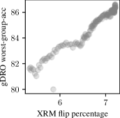
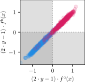
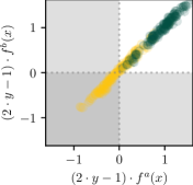
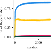
Figure 2: XRM on the Waterbirds problem, concerning   waterbirds in water,   waterbirds in land,   landbirds in water,   landbirds in land. The first panel shows that “percentage of XRM label flipped at convergence” is a strong indicator of “worst-group-accuracy in phase-2”, making flips a good criterion to select twin hyper-parameters. The two middle panels show the signed margin of the twins on each ground-truth group. From each of these class-dependent plots, XRM discovers two environments: one for points in the “mistake-free” white area, and one for points in the “cross-mistake” gray areas. Notably, XRM is able to allocate the two smallest groups    to dedicated environments. The fourth panel shows that label flipping happens almost exclusively for the two smallest groups, and stabilizes as training progresses.

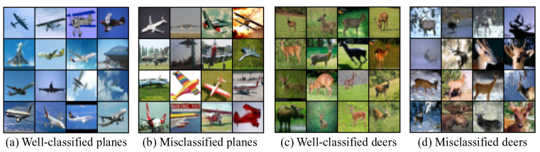
Figure 3: Randomly selected images of CIFAR-10 from groups identified by XRM. The twin networks show interesting patterns in their mistakes. Notably, well-classified examples are prototypical, such as planes against blue backgrounds and deers against a green backgrounds.

Figure 2 explores some of the behaviors of XRM on the Waterbirds dataset. In particular, the left panel justifies the use of “percentage of label flipped at convergence” as a phase-1 model selection criterion for XRM, as it correlates strongly with downstream phase-2 worst-group-accuracy. The two middle panels showcase the clear separation of the minority group “landbirds/water” by XRM, as no landbirds in land are in the cross-mistake area. The right panel shows that label flipping happens almost exclusively for minority groups, and converges alongside XRM training. This provides XRM with a degree of stability, removing the need for intricate early-stopping criteria.

Figure 3 applies XRM to the CIFAR-10 dataset (Krizhevsky et al., 2009). While CIFAR-10 does not contain environment annotations, the discovered environments by XRM for the “plane” and “deer” classes reveal one interesting spurious correlations, namely background color. As a final remark, we ablated the need for (i) holding-out data, and (ii) performing label flipping, finding that both components are essential to the performance of XRM.

6 Discussion

We have introduced Cross-Risk Minimization (XRM), a simple algorithm for environment discovery. XRM provides a recipe to tune its hyper-parameters, does not require early-stopping, and can discover environments for all training and validation data—dropping the requirement for human annotations at all. More specifically, XRM trains two twin label predictors on random halves of the training data, while encouraging each twin to imitate confident held-out mistakes by their sibling. This implements an “echo-chamber” that identifies environments that differ in spurious correlation, and endow domain generalization algorithms with oracle-like performance.

We highlight two directions for future work. Firstly, how does XRM relate to the invariance principle $Y\perp E\mid\Phi(X)$? What is the interplay between revealing relevant labels $Y$ and relevant environments $E$ as to afford invariance? To our knowledge, XRM is the first environment discovery algorithm tampering with labels $Y$, thus exploring invariance—and the violation thereof—from a new angle. Because relabeling happens with a probability proportional to confidence, we expect model calibration to play a role in understanding the theoretical underpinnings of XRM, as it happened with other invariance methods (Wald et al., 2021). Overall, the theoretical analysis of XRM will call for new tools, because the optimal solution is a moving target that depends on the dynamic evolution of the labels, steering away from the Bayes-optimal predictor $P(Y\mid X)$.

Secondly, we would like to further understand the relationship between XRM and the multifarious phenomenon of memorization. Good memorization affords invariance (Where did I park my car?), and therefore depends on the collection of environments deemed relevant. Bad memorization happens due to “structured over-fitting”, commonly incarnated as a bad learning strategy “use a simple feature for the majority, then memorize the minority”. XRM seems to attack a similar problem but, how does it specifically relate to these two flavours of memorization? Does XRM discover environments that promote features that benefit all examples?

Acknowledgements

We thank Kartik Ahuja, Martín Arjovsky, Léon Bottou, Kamalika Chaudhuri, Cijo Jose, Reyhane Askari Hemmat, Polina Kirichenko and others for fruitful discussions. We thank the FAIR leadership for their help in publishing this manuscript.

Appendix

Appendix A Experimental details

We follow the experimental protocol of SubpopBench [Yang et al., 2023]. Therefore, image datasets use a pretrained ResNet-50 [He et al., 2016] unless otherwise mentioned, and text datasets use a pretrained BERT [Devlin et al., 2018]. All images are resized and center-cropped to $224\times 224$ pixels, and undergo no data augmentation. We use SGD with momentum $0.9$ to learn from image datasets unless otherwise mentioned, and we employ AdamW [Loshchilov and Hutter, 2017] with default $\beta_{1}=0.9$ and $\beta_{2}=0.999$ for text benchmarks. For the ColorMNIST experiment [Arjovsky et al., 2019], we train a three-layer fully-connected network with layer sizes $[2*14*14,300,300,2]$ and use ReLU as the activation function. The network is optimized using the Adam optimizer with a learning rate of $1e-3$, and default parameters $\beta_{1}=0.9$ and $\beta_{2}=0.999$. For the experiment on CIFAR-10 [Krizhevsky et al., 2009], we train a VGG-16 model [Simonyan and Zisserman, 2014] using SGD with a learning rate of $1e-2$ and a momentum of $0.9$ We train XRM and phase-2 algorithms for a number of iterations that allows convergence within a reasonable compute budget. These are 5,000 steps for Waterbirds and Metashift, 10,000 steps for ImageNetBG, 20,000 steps for MultiNLI, and 30,000 steps for CivilComments.

A.1 Phase-1 XRM model selection

For phase-1, we run XRM with 16 random combinations of hyper-parameters, each over $k_{1}=10$ random seeds. (We repeat runs with null accuracy on one of the classes.) For each of the 16 hyper-parameter combinations, we average the number of flipped labels appearing at the last iteration (early-stopping is not necessary with XRM) across the 10 seeds. This will tell us which one of the 16 hyper-parameter combinations is best. For that combination, we average the training and validation logit matrices across the 10 random seeds. Finally, we discover environments using equation 4.

A.2 Phase-2 DG model selection.

For all phase-2 domain generalization algorithms (ERM, SUBG, RWG, GroupDRO), we search over 16 random combinations of hyper-parameters. We select the hyper-parameter combination and early-stopping iteration yielding maximal worst-group-accuracy (or, in the absence of groups, worst-class-accuracy). We re-run the best hyper-parameter combination for $k_{2}=10$ random seeds to report avg/std for test worst-group-accuracies (always computed with respect to the ground-truth group annotations). The $k_{1}$ random seeds from phase-1 do not contribute to error bars.

A.3 Hyper-parameter sampling grids

algorithm	hyper-parameter	ResNet	BERT
	learning rate	$10^{\text{Uniform}(-4,-2)}$	$10^{\text{Uniform}(-5.5,-4)}$
XRM, ERM,	weight decay	$10^{\text{Uniform}(-6,-3)}$	$10^{\text{Uniform}(-6,-3)}$
SUBG, RWG	batch size	$2^{\text{Uniform}(6,7)}$	$2^{\text{Uniform}(3,5.5)}$
	dropout	—	$\text{Random}([0,0.1,0.5])$
GroupDRO	$\eta$	$10^{\text{Uniform}(-3,-1)}$	$10^{\text{Uniform}(-3,-1)}$

Appendix B Learning to Split on Waterbirds

We benchmarked the official learning to split code-base https://github.com/YujiaBao/ls on the WaterBirds dataset. We assessed the method’s sensitivity to two hyperparameters: the number of epochs used for early stopping (patience argument in the codebase) and the pre-supposed ratio of groups (based on the ratio argument in the code). For patience we swept over (2, 5, 10) with 5 being the default value. For ratio, we swept over (0.25, 0.5, 0.75) with 0.75 being the default value based on the paper. We found worst group performance using a fixed GroupDRO phase-2 training varied by as much as $\pm 7\%{}$ on Waterbirds.

Appendix C Experimental results with error bars

lcccccccccccc papercolor!102-411-4 papercolor!102-711-7 papercolor!102-1011-10 papercolor!102-1311-13 ERM GroupDRO RWG SUBG
None Human XRM None Human XRM None Human XRM None Human XRM
Waterbirds 70.4 $\pm$2.99 76.1 $\pm$2.37 75.3 $\pm$1.96 71.7 $\pm$4.09 88.0 $\pm$2.61 86.1 $\pm$1.28 74.8 $\pm$2.50 87.0 $\pm$1.63 84.5 $\pm$1.53 73.0 $\pm$2.75 86.7 $\pm$1.00 76.3 $\pm$8.41
CelebA 62.7 $\pm$2.73 71.9 $\pm$3.48 67.6 $\pm$3.48 68.8 $\pm$1.29 89.1 $\pm$1.67 89.8 $\pm$1.39 70.7 $\pm$1.32 89.5 $\pm$1.45 88.0 $\pm$2.56 68.5 $\pm$2.13 87.1 $\pm$2.70 87.5 $\pm$2.54
MultiNLI 54.8 $\pm$4.04 65.3 $\pm$3.02 65.8 $\pm$3.41 69.7 $\pm$2.65 76.1 $\pm$1.29 74.3 $\pm$1.88 69.3 $\pm$1.77 71.1 $\pm$1.60 73.3 $\pm$1.56 53.7 $\pm$2.97 72.8 $\pm$0.66 71.3 $\pm$1.58
CivilComments 55.1 $\pm$3.46 59.7 $\pm$5.77 61.4 $\pm$4.48 59.3 $\pm$2.05 69.3 $\pm$2.32 71.3 $\pm$1.35 54.0 $\pm$4.58 65.8 $\pm$6.30 73.4 $\pm$0.93 58.7 $\pm$2.56 64.0 $\pm$7.63 72.9 $\pm$1.12
ColorMNIST 10.1 $\pm$0.51 10.1 $\pm$2.40 26.9 $\pm$2.27 10.0 $\pm$0.51 10.1 $\pm$2.37 70.5 $\pm$0.98 10.1 $\pm$0.51 10.2 $\pm$1.85 70.2 $\pm$1.00 10.1 $\pm$0.51 10.0 $\pm$2.21 70.8 $\pm$1.09
MetaShift 70.8 $\pm$2.99 67.7 $\pm$4.62 71.2 $\pm$3.95 70.8 $\pm$3.91 73.7 $\pm$4.42 71.2 $\pm$4.81 66.5 $\pm$4.55 70.8 $\pm$4.45 69.7 $\pm$4.86 70.0 $\pm$3.38 73.5 $\pm$3.49 69.2 $\pm$5.58
ImagenetBG 75.6 $\pm$3.04 76.9 $\pm$1.89 76.9 $\pm$1.93 73.0 $\pm$3.43 76.1 $\pm$1.40 75.9 $\pm$1.69 76.9 $\pm$2.42 76.5 $\pm$2.65 77.0 $\pm$2.66 75.0 $\pm$3.55 75.0 $\pm$3.55 76.4 $\pm$1.79

Appendix D XRM in PyTorch

⬇

1import torch

2

3def balanced_cross_entropy(p, y):

4 losses = torch.nn.functional.cross_entropy(p, y, reduction="none")

5 return sum([losses[y == yi].mean() for yi in y.unique()])

6

7def xrm(x_tr, y_tr, x_va, y_va, lr=1e-2, max_iters=1000):

8 # init twins, assign examples, and calibrate (Section 4.1)

9 nc = len(y_tr.unique())

10 net_a = torch.nn.Linear(x_tr.size(1), nc)

11 net_b = torch.nn.Linear(x_tr.size(1), nc)

12 ind_a = torch.zeros(len(x_tr), 1).bernoulli_(0.5).long()

13

14 # Platt temperature scaling

15 temp_a = torch.nn.Parameter(torch.ones(1, nc))

16 temp_b = torch.nn.Parameter(torch.ones(1, nc))

17 logits_a = net_a(x_tr).detach()

18 logits_b = net_b(x_tr).detach()

19 cal = torch.optim.SGD([temp_a, temp_b], lr)

20

21 for iteration in range(max_iters):

22 logits = logits_a / temp_a * ind_a + logits_b / temp_b * (1 - ind_a)

23 cal.zero_grad()

24 balanced_cross_entropy(logits, y_tr).backward()

25 cal.step()

26

27 net_a.weight.data.div_(temp_a.t().detach())

28 net_b.weight.data.div_(temp_b.t().detach())

29

30 # training (Section 4.2)

31 opt = torch.optim.SGD(

32 list(net_a.parameters()) + list(net_b.parameters()), lr)

33

34 for iteration in range(max_iters):

35 pred_a, pred_b = net_a(x_tr), net_b(x_tr)

36 pred_hi = pred_a * ind_a + pred_b * (1 - ind_a)

37 pred_ho = pred_a * (1 - ind_a) + pred_b * ind_a

38

39 opt.zero_grad()

40 balanced_cross_entropy(pred_hi, y_tr).backward()

41 opt.step()

42

43 # label flipping, useful for model selection (Section 4.3)

44 p_ho, y_ho = pred_ho.softmax(dim=1).detach().max(1)

45 is_flip = torch.bernoulli((p_ho - 1 / nc) * nc / (nc - 1)).long()

46 y_tr = is_flip * y_ho + (1 - is_flip) * y_tr

47

48 # environment discovery (Section 4.4)

49 cm = lambda x, y: torch.logical_or(

50 net_a(x).argmax(1).ne(y),

51 net_b(x).argmax(1).ne(y)).long().detach()

52

53 return cm(x_tr, y_tr), cm(x_va, y_va)

The code above may be helpful to clarify our exposition in the main text. For an end-to-end example running linear XRM and GroupDRO, see: https://pastebin.com/0w6gsxQw.

References

- Angwin et al. [2016] Julia Angwin, Jeff Larson, Surya Mattu, and Lauren Kirchner. Machine bias. ProPublica, 2016. https://www.propublica.org/article/machine-bias-risk-assessments-in-criminal-sentencing.
- Arjovsky et al. [2019] Martin Arjovsky, Léon Bottou, Ishaan Gulrajani, and David Lopez-Paz. Invariant risk minimization. arXiv, 2019. https://arxiv.org/abs/1907.02893.
- Bao and Barzilay [2022] Yujia Bao and Regina Barzilay. Learning to split for automatic bias detection. arXiv, 2022. https://arxiv.org/abs/2204.13749.
- Barocas et al. [2019] Solon Barocas, Moritz Hardt, and Arvind Narayanan. Fairness and Machine Learning: Limitations and Opportunities. fairmlbook.org, 2019. http://www.fairmlbook.org.
- Bojarski et al. [2016] Mariusz Bojarski, Davide Del Testa, Daniel Dworakowski, Bernhard Firner, Beat Flepp, Prasoon Goyal, Lawrence D Jackel, Mathew Monfort, Urs Muller, Jiakai Zhang, et al. End to end learning for self-driving cars. arXiv, 2016. https://arxiv.org/abs/1604.07316.
- Borkan et al. [2019] Daniel Borkan, Lucas Dixon, Jeffrey Sorensen, Nithum Thain, and Lucy Vasserman. Nuanced metrics for measuring unintended bias with real data for text classification. WWW, 2019. https://arxiv.org/abs/1903.04561.
- Bottou [2019] Léon Bottou. Learning representation with causal invariance. ICLR Keynote, 2019. https://leon.bottou.org/talks/invariances.
- Creager et al. [2020] Elliot Creager, Jörn-Henrik Jacobsen, and Richard Zemel. Environment inference for invariant learning. arXiv, 2020. https://arxiv.org/abs/2010.07249.
- Dagaev et al. [2021] Nikolay Dagaev, Brett D. Roads, Xiaoliang Luo, Daniel N. Barry, Kaustubh R. Patil, and Bradley C. Love. A too-good-to-be-true prior to reduce shortcut reliance. arXiv, 2021. https://arxiv.org/abs/2102.06406.
- DeGrave et al. [2021] Alex J DeGrave, Joseph D Janizek, and Su-In Lee. AI for radiographic COVID-19 detection selects shortcuts over signal. Nature Machine Intelligence, 2021. https://www.nature.com/articles/s42256-021-00338-7.
- Devlin et al. [2018] Jacob Devlin, Ming-Wei Chang, Kenton Lee, and Kristina Toutanova. Bert: Pre-training of deep bidirectional transformers for language understanding. arXiv preprint arXiv:1810.04805, 2018.
- Feldman and Zhang [2020] Vitaly Feldman and Chiyuan Zhang. What neural networks memorize and why: Discovering the long tail via influence estimation. arXiv, 2020. https://arxiv.org/abs/2008.03703.
- Geirhos et al. [2020] Robert Geirhos, Jörn-Henrik Jacobsen, Claudio Michaelis, Richard Zemel, Wieland Brendel, Matthias Bethge, and Felix A Wichmann. Shortcut learning in deep neural networks. Nature Machine Intelligence, 2020. https://arxiv.org/abs/2004.07780.
- Goodfellow et al. [2014] Ian J Goodfellow, Jonathon Shlens, and Christian Szegedy. Explaining and harnessing adversarial examples. arXiv, 2014. https://arxiv.org/abs/1412.6572.
- Goodman [1972] Nelson Goodman. Seven strictures on similarity. Problems and Projects, 1972. https://philpapers.org/rec/GOOSSO.
- Gulrajani and Lopez-Paz [2020] Ishaan Gulrajani and David Lopez-Paz. In search of lost domain generalization. arXiv, 2020. https://arxiv.org/abs/2007.01434.
- Guo et al. [2017] Chuan Guo, Geoff Pleiss, Yu Sun, and Kilian Q Weinberger. On calibration of modern neural networks. In ICML, 2017. https://arxiv.org/abs/1706.04599.
- Hand and Henley [1997] David J Hand and William E Henley. Statistical classification methods in consumer credit scoring: a review. Journal of the royal statistical society: series a (statistics in society), 1997. https://www.jstor.org/stable/2983268.
- He et al. [2016] Kaiming He, Xiangyu Zhang, Shaoqing Ren, and Jian Sun. Deep residual learning for image recognition. In Proceedings of the IEEE conference on computer vision and pattern recognition, pages 770–778, 2016.
- Heaven [2021] Will Douglas Heaven. Hundreds of AI tools have been built to catch COVID. none of them helped. MIT Technology Review, 2021. https://www.technologyreview.com/2021/07/30/1030329/machine-learning-ai-failed-covid-hospital-diagnosis-pandemic/.
- Idrissi et al. [2022] Badr Youbi Idrissi, Martin Arjovsky, Mohammad Pezeshki, and David Lopez-Paz. Simple data balancing achieves competitive worst-group-accuracy. CLeaR, 2022. https://arxiv.org/abs/2110.14503.
- Izmailov et al. [2022] Pavel Izmailov, Polina Kirichenko, Nate Gruver, and Andrew G Wilson. On feature learning in the presence of spurious correlations. NeurIPS, 2022. https://arxiv.org/abs/2210.11369.
- Japkowicz [2000] Nathalie Japkowicz. The class imbalance problem: Significance and strategies. In ICML, 2000. https://www.researchgate.net/publication/2639031_The_Class_Imbalance_Problem_Significance_and_Strategies.
- Jiang et al. [2017] Fei Jiang, Yong Jiang, Hui Zhi, Yi Dong, Hao Li, Sufeng Ma, Yilong Wang, Qiang Dong, Haipeng Shen, and Yongjun Wang. Artificial intelligence in healthcare: past, present and future. Stroke and vascular neurology, 2017. https://pubmed.ncbi.nlm.nih.gov/29507784/.
- Krizhevsky et al. [2009] Alex Krizhevsky, Vinod Nair, and Geoffrey Hinton. Cifar-10, 2009. http://www.cs.toronto.edu/~kriz/cifar.html.
- Lahoti et al. [2020] Preethi Lahoti, Alex Beutel, Jilin Chen, Kang Lee, Flavien Prost, Nithum Thain, Xuezhi Wang, and Ed H. Chi. Fairness without demographics through adversarially reweighted learning. arXiv, 2020. https://arxiv.org/abs/2006.13114.
- Liang and Zou [2022] Weixin Liang and James Zou. Metashift: A dataset of datasets for evaluating contextual distribution shifts and training conflicts. arXiv, 2022. https://arxiv.org/abs/2202.06523.
- Liu et al. [2015] Ziwei Liu, Ping Luo, Xiaogang Wang, and Xiaoou Tang. Deep learning face attributes in the wild. In ICCV, 2015. https://arxiv.org/abs/1411.7766.
- Lopez-Paz et al. [2022] David Lopez-Paz, Diane Bouchacourt, Levent Sagun, and Nicolas Usunier. Measuring and signing fairness as performance under multiple stakeholder distributions. arXiv, 2022. https://arxiv.org/abs/2207.09960.
- Loshchilov and Hutter [2017] Ilya Loshchilov and Frank Hutter. Decoupled weight decay regularization. arXiv preprint arXiv:1711.05101, 2017.
- Nam et al. [2020] Junhyun Nam, Hyuntak Cha, Sungsoo Ahn, Jaeho Lee, and Jinwoo Shin. Learning from failure: Training debiased classifier from biased classifier. arXiv, 2020. https://arxiv.org/abs/2007.02561.
- Qiu et al. [2023] Shikai Qiu, Andres Potapczynski, Pavel Izmailov, and Andrew Gordon Wilson. Simple and fast group robustness by automatic feature reweighting. arXiv, 2023. https://arxiv.org/abs/2306.11074.
- Sagawa et al. [2019] Shiori Sagawa, Pang Wei Koh, Tatsunori B. Hashimoto, and Percy Liang. Distributionally robust neural networks for group shifts: On the importance of regularization for worst-case generalization. ICLR, 2019. https://arxiv.org/abs/1911.08731.
- Shah et al. [2020] Harshay Shah, Kaustav Tamuly, Aditi Raghunathan, Prateek Jain, and Praneeth Netrapalli. The pitfalls of simplicity bias in neural networks. NeurIPS, 2020. https://arxiv.org/abs/2006.07710.
- Simonyan and Zisserman [2014] Karen Simonyan and Andrew Zisserman. Very deep convolutional networks for large-scale image recognition. arXiv preprint arXiv:1409.1556, 2014.
- Vapnik [1998] Vladimir Vapnik. Statistical learning theory. Wiley, 1998. https://www.wiley.com/en-us/Statistical+Learning+Theory-p-9780471030034.
- Wah et al. [2011] Catherine Wah, Steve Branson, Peter Welinder, Pietro Perona, and Serge Belongie. The Caltech-UCSD birds-200-2011 dataset. California Institute of Technology, 2011. https://www.vision.caltech.edu/datasets/cub_200_2011/.
- Wald et al. [2021] Yoav Wald, Amir Feder, Daniel Greenfeld, and Uri Shalit. On calibration and out-of-domain generalization. NeurIPS, 2021. https://arxiv.org/abs/2102.10395.
- Wang et al. [2021] Jindong Wang, Cuiling Lan, Chang Liu, Yidong Ouyang, Tao Qin, Wang Lu, Yiqiang Chen, Wenjun Zeng, and Philip S. Yu. Generalizing to unseen domains: A survey on domain generalization. arXiv, 2021. https://arxiv.org/abs/2103.03097.
- Williams et al. [2017] Adina Williams, Nikita Nangia, and Samuel R Bowman. A broad-coverage challenge corpus for sentence understanding through inference. ACL, 2017. https://aclanthology.org/N18-1101/.
- Xiao et al. [2020] Kai Xiao, Logan Engstrom, Andrew Ilyas, and Aleksander Madry. Noise or signal: The role of image backgrounds in object recognition. arXiv, 2020. https://arxiv.org/abs/2006.09994.
- Yang et al. [2023] Yuzhe Yang, Haoran Zhang, Dina Katabi, and Marzyeh Ghassemi. Change is hard: A closer look at subpopulation shift. arXiv, 2023. https://arxiv.org/pdf/2302.12254.pdf.
- Zheran Liu et al. [2021] Evan Zheran Liu, Behzad Haghgoo, Annie S. Chen, Aditi Raghunathan, Pang Wei Koh, Shiori Sagawa, Percy Liang, and Chelsea Finn. Just train twice: Improving group robustness without training group information. arXiv, 2021. https://arxiv.org/abs/2107.09044.
- Zhou et al. [2022] Kaiyang Zhou, Ziwei Liu, Yu Qiao, Tao Xiang, and Chen Change Loy. Domain generalization: A survey. IEEE PAMI, 2022. https://arxiv.org/abs/2103.02503.