Anomalous Purcell decay of strongly driven inhomogeneous emitters coupled to a cavity

We perform resonant fluorescence lifetime measurements on a nanocavity-coupled erbium ensemble as a function of cavity-laser detuning and pump power. Our measurements reveal an anomalous suppression of the ensemble decay lifetime at zero cavity detuning and high pump fluence. We capture qualitative aspects of this decay rate suppression using a Tavis-Cummings model of non-interacting spins coupled to a common cavity.

1 Introduction

Tailoring the interaction between atoms and their electromagnetic environment is of both fundamental interest and practical relevance, e.g., for applications in quantum communication and quantum information processing [1, 2]. By tuning the photon density of states, one can drastically modify the emission properties of atoms [3], a phenomena that underpins the thriving research area of cavity quantum electrodynamics (cQED) [4]. Prototypical cases (for which even analytical solutions often exist) are the interaction between a single two-level system (which we will interchangeably refer to as a “spin”) and a single mode of a radiation field [5], the collective interaction of atoms with their electromagnetic environment leading to the effects of super- and subradiance [6, 7, 8], as well as photon-mediated collective interactions [9], and large ensembles of weakly excited spins with identical or inhomogeneously broadened transition frequencies [5, 10]. The limit where the spins are only weakly perturbed away from their ground or excited states is appealing, since the spin dynamics become linear and analytical studies of the dynamics become possible [11, 12, 13]. Much less is known, however, in the case of highly excited spins where the intrinsic nonlinearity of the spin dynamics due to their finite-dimensional Hilbert space needs to be taken into account.

Trapped atomic systems are the prototypical spin for investigating optical relaxation dynamics because of their coherence and homogeneity in ensembles. In cQED, there is particular interest in modifying the atom-photon coupling strength through the use of high quality factor (Q) and small mode volume optical cavities. While significant progress has been made in integrating conventional trapped atomic systems with these types of resonators [14, 15, 16], it still remains an outstanding technical challenge to experimentally achieve high coupling with modest ensembles of atoms to probe the rich phenomena available from collective effects[17, 18, 19, 20]. In contrast, rare-earth ions embedded in solid-state hosts and integrated with nanoscale optical cavities—which are being explored for use in quantum memories[21, 22, 23, 24] and microwave-to-optical transduction[25, 26], have naturally long optical lifetimes that are ideally suited for optical decay modification experiments. These features of nanocavity-coupled rare-earths are typically at the expense of large inhomogeneous broadening, but this trait has recently been shown to be an important factor in the observation of collectively induced transparency[27], where the dynamics of a strongly driven and disordered ensemble can modify the steady-state system response due to an interplay of quantum interference and collective effects. Similarly in this work, we study an ensemble of rare-earth ions coupled to a relatively high Q, small mode volume optical cavity and subjected to a resonant laser driving field. The large inhomogeneous linewidth of the ensemble, and the relatively narrow resonance of the cavity, enable us to explore interesting modification behavior in the optical relaxation of the highly excited spins—as a function of both cavity-laser detuning and optical drive power—likely a regime where the collective cooperativity is large and disorder plays a non-trivial role.

Our specific spin-cavity system consists of trivalent erbium ions (Er³⁺ or Er for brevity) incorporated into a thin layer of TiO₂ grown atop silicon-on-insulator wafers[28, 29]. The Er ions are evanescently coupled to a 1D photonic crystal cavity that is patterned through both the TiO₂ and Si device layers. In a prior study, we attempted to measure the Purcell enhancement in Er-doped TiO₂ films coupled to a nanophotonic cavity as we tuned the cavity resonance across a particular optical transition[28]. During the course of those experiments, we noticed features resembling the saturation of the Purcell enhancement at high laser pump powers. However, the overall photon collection efficiency and fluorescence signal were too low to perform sufficient sweeps of the optical drive. Here, the Er concentration is three-fold increased by growing more highly doped films and the device-to-fiber coupling efficiency is five-fold increased by incorporating an inverse taper in-coupling structure. We report anomalously slow relaxation rates in the temporal response of highly-excited and inhomogeneously broadened spin ensembles. Finally, we develop a simple theoretical model to explain the qualitative features in the Purcell-enhanced ensemble decay.

2 Experimental details and results

2.1 Samples and device fabrication

For this study, we use molecular beam deposited Er-doped TiO₂ films that contain both rutile and anatase crystalline grains, as was seen previously[28]. Previous experiments have shown that the inclusion of undoped layers surrounding a doped region can reduce optical inhomogeneous broadening for epitaxial Er:Y₂O₃ [30] and Er:TiO₂ thin films[31], as well as spectral diffusion and inhomogeneous linewidth broadening for Er in polycrystalline TiO₂ films[32]. However, a thicker TiO₂ layer is more difficult to etch anisotropically into high Q cavities. With both of these considerations in mind, we use a ‘$10/10/10$’ heterostructure: a 10 nm undoped TiO₂ buffer layer at the Si interface, a 10 nm Er-doped TiO₂ layer in the middle, and a 10 nm undoped TiO₂ capping layer on top. The sample is grown on a standard SOI wafer used for silicon photonics. During the molecular beam deposition of Er:TiO₂, we use a substrate temperature of 390 ^∘C and metallic Er cell temperature of 900 ^∘C. This Er temperature corresponds to flux that will yield 120 (130) ppm Er if the crystal phase of the TiO₂ is rutile (anatase) due to the difference in density.

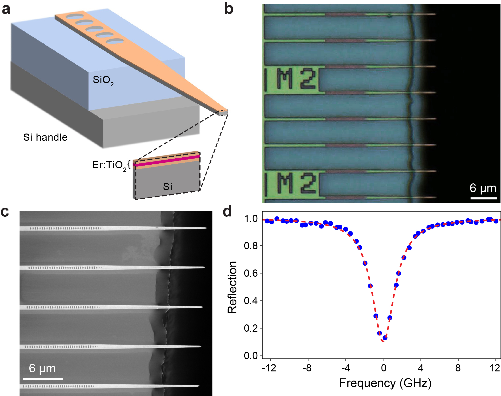
Figure 1: Er-doped TiO₂-Si 1D photonic crystal cavities. (a) Schematic of our fabricated devices showing the inverse taper of the waveguide extending off the chip. The inset at the end facet highlights the doped TiO₂ heterostructure deposited on top of the Si device layer consisting of 10 nm of undoped TiO₂/10 nm doped TiO₂ ($\sim 120$ ppm Er, colored red)/10 nm undoped TiO₂. (b) Top view optical image of fully fabricated devices after the multi-step undercut process. (c) Scanning electron microscope image on the same chip as (b) highlighting the nanophotonic cavity composed of elliptically shaped holes etched through the TiO₂ and Si device layers. (d) Normalized laser reflection spectrum of the cavity tuned onto resonance with the $Z_{1}\rightarrow Y_{1}$ optical transition for Er in rutile phase TiO₂ ($\lambda=1520.52$ nm) at a sample temperature of 3.5 K. Using a Lorentzian fit (red dashed line), the cavity quality factor gives Q=$(6.71\pm 0.11)\times 10^{4}$.

Our Er:TiO₂/Si photonic crystal cavities are optically addressed in a one-sided configuration via lensed optical fiber. The waveguide width and photonic crystal cavity design parameters are identical to that shown previously[28]. However, for this work we wanted to improve the coupling efficiency between the lensed fiber and the cavity, as previous devices involved end-fire coupling into a cleaved waveguide with an efficiency of $10-15\%$. To do so, we used Lumerical 3D FDTD simulations to optimize the design of an inverse taper that extends off the edge of the chip (Fig. 1a) for better mode matching to the lensed fiber[33, 34] (simulation details are provided in the Supplementary Information (SI)). The simulations show that an adiabatic reduction in waveguide width from 650 nm (where the cavity holes end) down to 200 nm over a 14 $\mu$m length, allows for a fiber coupling efficiency up to $80\%$.

We fabricate these Er:TiO₂ on Si 1D photonic crystal cavities as outlined previously[28], but with additional steps to selectively undercut the inverse tapers without damaging the Si and TiO₂ (complete fabrication flow is provided in Fig. S2, SI). We deposit a device protection layer of conformal thermal ALD alumina, which covers the top surface of the sample as well as the exposed sidewalls and end facet of the inverse taper. We then cleave the SOI chip adjacent to the termini of the tapers via a precision cleaver under an optical microscope. After this, we perform an isotropic etch of the Si handle layer via XeF₂ etching, followed by vapor HF (VHF) etching to undercut the buried SiO₂. After sufficient VHF exposure to fully remove the 2 $\mu$m buried oxide layer underneath the suspended portion of the taper, we strip the protective alumina layer using a wet etchant and anneal the sample. Optical and SEM images of the final devices are shown in Figures 1b and 1c, respectively. It should be noted that as long as the vapor processes yield a lateral undercut length of at least 4 $\mu$m of the 14 $\mu$m taper (like those shown in Fig. 1b-c), the mode is sufficiently waveguided such that minimal light is lost into the substrate (Fig. S1a, SI).

2.2 Optical measurements at 3.5 K

We perform our optical device measurements in a fiber-accessible cryostat at a sample temperature of 3.5 K, and the experimental configuration is discussed elsewhere[28]. For this work, we will explore ensemble cavity coupling to the $Z_{1}\rightarrow Y_{1}$ optical transition for Er in rutile phase TiO₂ ($\lambda=1520.52$ nm) [35]. We then use a continuous-wave (CW) tunable laser (Toptica CTL 1550) to sweep through the device resonance and measure the continuous wave reflection spectrum for the cavity. The cavity full-width half-maximum (FWHM) linewidth is $2.94\pm 0.05$ GHz, when centered at $\lambda=1520.52$ nm, and this corresponds to a Q =$(6.71\pm 0.11)\times 10^{4}$ (Fig. 1d) with a waveguide-cavity mode coupling efficiency, $\eta$ =34%, yielding a decay rate from the cavity of $\kappa_{\mathrm{c}}=0.34\kappa$. In a simplified ambient setup with a closed-loop nanopositioner, we measure our updated in-coupling structures to have a typical lensed fiber-to-waveguide coupling efficiency of $\approx 75\%$, which is close to our simulated maximum of $80\%$. However, when we perform the same characterization in the cryostat at 3.5 K, we see values closer to $\approx 65\%$.

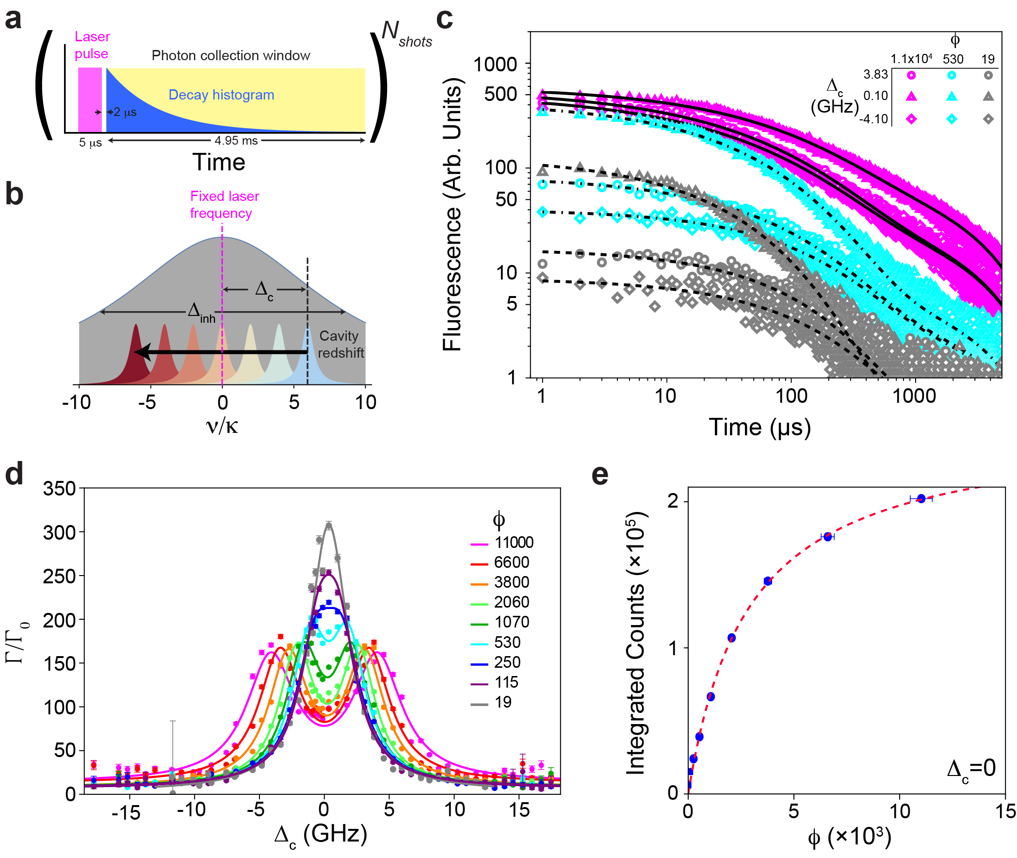
Figure 2: PLE Measurements on cavity-coupled Er ensembles at 3.5 K. (a) Schematic of our photoluminescence excitation measurement sequence. We first generate a 5 $\mu$s long laser excitation pulse (magenta). After a 2 $\mu$s wait time, we open an additional modulator in the collection path to start the photon collection window (yellow) to enable detection of the fluorescence from the ensemble. This single pulse sequence is repeated over $N_{shots}$ measurements to build up a histogram of the decay (blue). (b) Schematic of the cavity tuning mechanism in the measurement. For all of these measurements the laser is locked to a particular frequency at the center of the ensemble’s inhomogeneous distribution. This distribution is broad relative to the cavity linewidth ($\kappa$) and is represented by the wide gray Lorentzian ($\approx 17\kappa$). The cavity is slowly redshifted through the resonance through gas condensation tuning, and its frequency relative to the laser is given by $\Delta_{\mathrm{c}}$. The experimental extent of $\Delta_{\mathrm{c}}$ is $\approx 12\kappa$ as represented with the blue-to-red transition of the cavity Lorentzian. (c) Nine example experimental time traces for three different incident photon flux values ($\phi$) and cavity-laser detuning values ($\Delta_{\mathrm{c}}$). The various black lines are fits to the experimental data as described in the main text. (d) The spontaneous decay rate enhancement ($\Gamma/\Gamma_{0}$) as a function of the cavity-laser detuning ($\Delta_{\mathrm{c}}$) for increasing photon fluxes ($\phi$). The $\Gamma/\Gamma_{0}$ values are extracted from the stretched exponential time constants fit to experimental data such as those in (c). The solid lines for each flux are from a pair of Lorentzian lineshapes fit to the experimental data. (e) Measurements of the integrated fluorescence intensity when the cavity is resonant with the optical transition ($\Delta_{\mathrm{c}}$ = 0.10 GHz), the red dashed line is a saturation fit as described in the main text.

We explore the cavity-coupled optical relaxation dynamics in these ensembles using resonant photoluminescence excitation (PLE) measurements as depicted in Figure 2a. We use three acousto-optic modulators (AOM) in series to generate 5 $\mu$s laser pulses from our tunable CW laser. After the end of the laser pulse, we wait 2 $\mu$s before opening a fourth AOM in the collection path to our superconducting nanowire single-photon detectors (SNSPDs), which are not gated. We can repeat each pulse sequence many times (typically 4000 shots) to create a histogram of the ensemble fluorescence lifetime and measure the integrated intensity. Using this approach, resonant PLE from a laser sweep near 1520.52 nm, yields a broad Er³⁺ ensemble linewidth of 50 GHz, as was shown previously[28], and is represented by the wide gray Lorentzian shown in Figure 2b. The inhomogeneous linewidth $\Delta_{\mathrm{inh}}$ is much broader than the cavity linewidth ($\kappa$=2.94 $\pm$ 0.05 GHz), and we use nitrogen gas condensation on the cavity to tune the refractive index and slowly redshift the cavity resonance through the center of the inhomogeneous linewidth. For the majority of measurements, the laser is locked at $\lambda=1520.52$ nm using a wavemeter (WS-8-10, High Finesse) calibrated against a fixed frequency reference laser (SLR-1532, High Finesse). We periodically interrupt PLE measurements to perform CW laser reflection measurements, such as the one shown in Figure 1d, to precisely measure the cavity-laser detuning parameter, $\Delta_{\mathrm{c}}$. Given that the inhomogeneous linewidth of the Er in rutile $Z_{1}\rightarrow Y_{1}$ transition is broad, it is important to investigate if the homogeneous linewidth of these emitters is sufficiently narrow to enable cavity-based lifetime enhancement (‘bad cavity’ limit). Similar to previous work[28], we have performed transient spectral hole burning (TSHB) measurements at 3.5 K, to find an upper bound on the homogeneous and spectral diffusion linewidths[36], as shown in Figure S3 of the SI. We can see that for the range of relevant incident photon fluxes for which we see TSHB contrast, the TSHB linewidth is $\leq 0.3$ GHz, and we assume that for even higher fluxes our cavity-coupled ensemble remains in the ‘bad cavity’ regime.

We can now perform lifetime measurements at a variety of input laser powers for each cavity detuning. For later comparison with theory, we quantify the incident laser brightness in terms of $\phi$, the photon flux incident on the cavity per cavity lifetime (1/$\kappa$). It is important to note that for a given detuning we perform a full sweep of the incident fluxes and then measure the cavity reflection to gauge the resonance position. The cavity tuning rate is sufficiently slow to enable us to average our resultant lifetime histograms over five power sweeps, as this is useful in achieving sufficient detected photon numbers for the lower flux measurements, as well as averaging over fluctuations in the total intensity, as will be discussed later. As shown in Figure 2c, for the lowest laser power used ($\phi=19$) we measure a fast decay time close to resonance ($\Delta_{\mathrm{c}}\approx 0$) and slower decay at modest cavity detunings of $\approx\pm 4$ GHz. In contrast, even though the fluorescence intensity is brighter for the highest laser power ($\phi=1.1\times 10^{4}$), we see faster decay when the cavity is detuned from the transition than on resonance. Following previous work[28, 27], we can fit the experimental data using a function of the form: $A\exp[-(t/\tau_{1})^{d}]+B\exp(-t/\tau_{2})+C$. For our case, the stretched exponential with lifetime $\tau$ represents the fastest ensemble fluorescence decay rate ($\Gamma=1/\tau$) mediated by coupling the cavity. The stretching exponent attempts to capture the distribution of individual ion-cavity coupling strengths ($g$) within the ensemble, and the single exponential represents slower decay from Er ions along the inverse taper waveguide because the ions are located everywhere in the film[28]. If we also measure the optical lifetime of the fluorescence decay rate in a bare waveguide without a cavity $\Gamma_{0}$ (Fig. S4, SI), then the cavity-mediated Purcell enhancement, $\Gamma/\Gamma_{0}$, can be computed for each incident flux and cavity detuning, and the resultant plot is shown in Figure 2d. Most interesting is that at higher incident fluxes we see a double-peak decay profile appear, the decay rate appears to slow when the cavity is resonant with the driving field. This double-peaked detuning profile is significantly wider than the lower power cases: a single Lorentzian fit of the $\phi=19$ case yields a FWHM = $3.96\pm 0.24$, which is 35% wider than the cavity linewidth measured via reflection. However, if we integrate all photons detected at a particular detuning for each flux (regardless of time bin), the commensurate normalized intensity versus detuning plot does not show this double-lobed structure (Fig. S5 in the SI). Instead, all curves are qualitatively similar with comparable widths (FHWM $\sim 5$ GHz).

When we plot the total PLE intensity for the resonant case, we can see the onset of saturation (Fig. 2e), where the dashed red line is a fit to a standard photoluminescence-excitation (PLE) function of the form

$$P(\phi)=\frac{p_{1}}{p_{2}+1/\phi}~{}.$$ (1)

If we use the total experimental photon collection efficiency of our system (0.023) and the detected number of photons, we can infer $\sim 2200$ photons generated in the cavity per pulse at the highest pump power ($\phi=1.1\times 10^{4}$). Since we are in a saturation regime, we can generally conclude that the number of ions that are addressed with our optical pulse is close to this value. Using our device geometry and doping density, we very coarsely estimate that there are $7\times 10^{4}$ total ions along the cavity, though our uncertainty is quite large given the unknown proportion of Er ions residing in the rutile vs anatase grains. However, if we use this value and make another coarse estimate that if the spectral window that is being addressed with these highest power pulses is approximately the cavity linewidth ($\kappa$=2.94 GHz), then we expect $\sim 2600$ ions to couple. Since our estimates on ion number and photons generated in the cavity are reasonably close (in a regime where the ensemble appears to be saturating) we expect that the number of participating ions is close to 2000, and this estimate is useful in conducting simulations to explain the features in the Purcell factor detuning dependence.

3 Theory and discussion

3.1 Semiclassical model

To model the interaction between the nanophotonic cavity and the Er ions coupled to it, we treat each ion as a two-level system, representing the $Z_{1}$ and $Y_{1}$ levels, which is interacting with the cavity mode via a standard Tavis-Cummings interaction,

$$\hat{H}=\Delta_{\mathrm{c}}\hat{a}^{\dagger}\hat{a}+\sum_{j=1}^{N}\delta_{j}\frac{\hat{\sigma}_{z}}{2}+\sum_{j=1}^{N}g_{j}\left(\hat{a}^{\dagger}\hat{\sigma}_{-}^{j}+\hat{a}\hat{\sigma}_{+}^{j}\right)-i\sqrt{\kappa_{\mathrm{c}}}\beta_{\mathrm{in}}\left(\hat{a}^{\dagger}-\hat{a}\right)~{}.$$ (2)

Here, $\hat{\sigma}_{z}^{j}$ is the Pauli $z$ matrix of ion $j$, $\hat{\sigma}_{\pm}^{j}$ are the associated spin raising and lowering operators, respectively, and $\hat{a}$ is the lowering operator of the cavity mode. The cavity is driven by a laser at frequency $\omega_{\mathrm{dr}}$ which generates an input photon flux $\phi=|\beta_{\mathrm{in}}|^{2}$. We work in a frame rotating at the drive frequency and $\Delta_{\mathrm{c}}=\omega_{\mathrm{c}}-\omega_{\mathrm{dr}}$ ($\delta_{j}=\omega_{j}-\omega_{\mathrm{dr}}$) is the corresponding detuning of the cavity (ion $j$). Relaxation of each ion and damping of the cavity are described by the quantum master equation

$$\frac{\mathrm{d}}{\mathrm{d}t}\hat{\rho}=-i\left[\hat{H},\hat{\rho}\right]+\kappa\mathcal{D}[\hat{a}]\hat{\rho}+\gamma\sum_{j=1}^{N}\mathcal{D}[\hat{\sigma}_{-}^{j}]\hat{\rho}~{},$$ (3)

where $\mathcal{D}[\hat{o}]\hat{\rho}=\hat{o}\hat{\rho}\hat{o}^{\dagger}-\left\{\hat{o}^{\dagger}\hat{o},\hat{\rho}\right\}/2$ is a Lindblad dissipator. Here, $\gamma$ is the relaxation rate of the ions and $\kappa$ is the total cavity damping rate, which accounts for the damping rate $\kappa_{\mathrm{c}}$ due to the input port (through which the drive laser enters the cavity) and other internal losses.

Since it is intractable to solve the quantum master equation (3) for large ensembles of ions, we derive equations of motion for the coherent cavity field $a=\langle\hat{a}\rangle$ as well as the spin populations $s_{z}^{j}=\langle\hat{\sigma}_{z}^{j}\rangle$ and coherences $s_{-}^{j}=\langle\hat{\sigma}_{-}^{j}\rangle$. Because of the nonlinearity of the spins, these equations of motion will not form a closed set of differential equations. We therefore perform a semiclassical approximation $\langle\hat{o}_{1}\hat{o}_{2}\rangle\approx\langle\hat{o}_{1}\rangle\langle\hat{o}_{2}\rangle$ [37], also known as a first-order mean-field approximation, which leads to

$$\frac{\mathrm{d}}{\mathrm{d}t}a =-\left(i\Delta_{\mathrm{c}}+\frac{\kappa}{2}\right)a-i\sum_{j=1}^{N}g_{j}s_{-}^{j}-\sqrt{\kappa_{\mathrm{c}}}\beta_{\mathrm{in}}~{},$$ (4)

$$\frac{\mathrm{d}}{\mathrm{d}t}s_{-}^{j} =-\left(i\delta_{j}+\frac{\gamma}{2}\right)s_{-}^{j}+ig_{j}as_{z}^{j}~{},$$ (5)

$$\frac{\mathrm{d}}{\mathrm{d}t}s_{z}^{j} =2ig_{j}\left[a^{*}s_{-}^{j}-a(s_{-}^{j})^{*}\right]-\gamma(1+s_{z}^{j})~{}.$$ (6)

Even though this approximation neglects all correlations between the cavity field and the spins and does not take into account the presence of the ions coupled to the inverse taper, the resulting equations of motion are still able to capture the relevant qualitative aspects of the experimental data, as we will show below.

To simulate the dynamics of a disordered ensemble of ions, we randomly draw the detunings $\delta_{j}$ of $N-1$ ions from a Lorentzian distribution $L(\delta,\tilde{\delta},h)=h/\pi[(\delta-\tilde{\delta})^{2}+h^{2}]$, centered around $\tilde{\delta}=0$ with a full-width-at-half-max (FWHM) of $2h=\Delta_{\mathrm{inh}}$. The remaining last ion is always chosen to be resonant with the drive. Similarly, we randomly draw the coupling strengths $g_{j}$ of each ion from a Gauss distribution $G(g,\overline{g},\sigma)=\exp[-(g-\overline{g})^{2}/2\sigma^{2}]/\sqrt{2\pi}\sigma$ with mean coupling strength $\bar{g}$ and standard deviation $\sigma$. This procedure ensures that the detunings $\delta_{j}$ and the couplings $g_{j}$ of each ion are uncorrelated random variables. Since a finite number of spins is in general not sufficient to smoothly sample a broad inhomogeneous frequency distribution, we repeat this procedure $n_{\mathrm{traj}}$ times to generate a set of random disorder realizations. For each of these disorder realizations, we initialize the cavity in the vacuum state and the ions in the ground state, i.e., $a=s_{-}^{j}=0$ and $s_{z}^{j}=-1$, and evolve the semiclassical equations of motion (4) to (6) with the laser drive switched on, $\beta_{\mathrm{in}}>0$, for a time $t_{\mathrm{pulse}}$. Subsequently, we use the final state at $t_{\mathrm{pulse}}$ as the new initial state for a simulation of the fluorescence of the ion ensemble, where the laser drive has been switched off, $\beta_{\mathrm{in}}=0$. The semiclassical output field of the cavity is $a_{\mathrm{out}}=\sqrt{\kappa_{\mathrm{c}}}a+\beta_{\mathrm{in}}$, and the photon flux impinging on a photodetector measuring the output mode is $|a_{\mathrm{out}}|^{2}$.

For the numerical simulations, we choose parameters that are inspired by the corresponding experimental values but allow us to perform efficient simulations of the inhomogeneously broadened spin ensemble. Based on the transient-spectral-hole-burning experiments, we choose the spin decay rate to be $\gamma=0.005\kappa$. In order to get a larger output mode amplitude, we increase the output coupling strength compared to the experimental value and use $\kappa_{\mathrm{c}}=0.8\kappa$. We reduce the width of the inhomogeneous distribution to $\Delta_{\mathrm{inh}}=5\kappa$ to be able to perform disorder averages using $N=61$ ions and $n_{\mathrm{traj}}=120$ random disorder realizations. Since the experimental value of the coupling strength of the ions is unknown, we choose $\overline{g}=0.07\kappa$ such that $C=4N\overline{g}^{2}/\kappa\gamma\gg 1$ should allow us to resolve collective effects in the simulations.

3.2 Explicit form of the state prepared by excitation pulse

The state of the ion ensemble at the end of the excitation pulse can be well understood using an argument that combines single-spin (i.e., local) dynamics and the concept of collectively induced transparency (CIT), which has recently been introduced and experimentally demonstrated[27]. For an excitation pulse that is long compared to both the cavity decay timescale $1/\kappa$ and the intrinsic spin decay timescale $1/\gamma$, the system will approach a drive-dependent steady state. After eliminating the spin coherence $s_{-}^{j}$ by solving for the steady state of Eq. (5), one finds that the steady-state cavity field and the spin excitations are given by the self-consistent solution of

$$a_{\mathrm{ss}} =\frac{i\sqrt{\kappa_{\mathrm{c}}}\beta_{\mathrm{in}}}{\Delta_{\mathrm{c}}-i\frac{\kappa}{2}+\sum_{j=1}^{N}\frac{g_{j}^{2}}{\delta_{j}-i\gamma/2}s_{z,\mathrm{ss}}^{j}}~{},$$ (7)

$$s_{z,\mathrm{ss}}^{j} =-\left(1+\frac{2g_{j}^{2}}{\delta_{j}^{2}+\gamma^{2}/4}|a_{\mathrm{ss}}|^{2}\right)^{-1}~{}.$$ (8)

The last term in the denominator of Eq. (7) represents a spin-excitation-dependent self energy that can renormalize both the effective detuning $\Delta_{\mathrm{c}}$ and the decay rate $\kappa$ of the cavity. In the limit of weakly excited spins, $s_{z}^{j}\approx-1$, Eq. (7) can be averaged over the disorder distributions $L(\delta,0,\Delta_{\mathrm{inh}}/2)$ and $G(g,\overline{g},\sigma)$,

$$\overline{a}_{\mathrm{ss}}=\frac{i\sqrt{\kappa_{\mathrm{c}}}\beta_{\mathrm{in}}}{\Delta_{\mathrm{c}}-i\left[\frac{\kappa}{2}+\frac{2N_{\mathrm{eff}}(\overline{g}^{2}+\sigma^{2})}{\gamma+\Delta_{\mathrm{inh}}}\right]}~{},$$ (9)

i.e., the disorder-averaged self-energy is purely imaginary and merely renormalizes the cavity decay rate. Here, $N_{\mathrm{eff}}<N$ is the effective number of ions in the ensemble that contribute to the sum in Eq. (7), i.e., those ions that have not been depolarized into a state with $s_{z}^{j}\approx 0$. This results also reveals that the relevant collective cooperativity that controls renormalizations of the bare cavity damping rate $\kappa$ due to its interaction with the spin ensemble is $C_{\mathrm{inh}}=4N_{\mathrm{eff}}\overline{g}^{2}/\Delta_{\mathrm{inh}}\kappa$, where we assumed $\sigma^{2}\ll\overline{g}^{2}$ and $\gamma\ll\Delta_{\mathrm{inh}}$. Even though the collective cooperativity $C$ may be large, $C_{\mathrm{inh}}\approx 0.24$ is only modest due to the large inhomogeneous broadening $\Delta_{\mathrm{inh}}$. Surprisingly, this result provides an excellent description of the disorder-averaged steady-state cavity field even in the limit of strong driving, where spins resonant with the drive laser are almost depolarized, $s_{z}^{j}\to 0$. An intuitive explanation is the CIT effect [27]: For $|\overline{a}_{\mathrm{ss}}|g_{j}\gg\gamma$, ions in a window $|\delta_{j}|\ll|\overline{a}_{\mathrm{ss}}|g_{j}$ around the drive laser frequency will be highly depolarized, $s_{z}^{j}\approx 0$, and their contributions to the self energy term in Eq. (7) will be suppressed. Consequently, the self-energy will be dominated by spins with a large detuning $|\delta_{j}|\gg|\overline{a}_{\mathrm{ss}}|g_{j}$, but these spins have $s_{z}^{j}\approx-1$ such that the weak-drive assumption used to derive Eq. (9) remains valid if $N_{\mathrm{eff}}$ is suitably adjusted. For our numerical parameters, the renormalization of the cavity decay rate by the self-energy term is less than $24\%$ due to the small value of $C_{\mathrm{inh}}$.

Given the analytical expression (9), we decompose the cavity field into its semiclassical disorder-averaged steady-state value and quantum fluctuations $\hat{d}$, $\hat{a}=\overline{a}_{\mathrm{ss}}+\hat{d}$ and find that, to leading order, $\hat{H}$ decouples into a sum of $N$ independent single-spin Hamiltonians $\hat{H}_{j}=\delta_{j}\hat{\sigma}_{z}^{j}/2+g_{j}(\overline{a}_{\mathrm{ss}}^{*}\hat{\sigma}_{-}^{j}+\overline{a}_{\mathrm{ss}}\hat{\sigma}_{+}^{j})$, each describing a coherent Rabi drive. This Rabi drive competes with single-spin relaxation and detuning $\delta_{j}$ such that each spin relaxes to a steady state with

$$s_{z,\mathrm{ss}}^{j} =-1+\frac{8|\overline{a}_{\mathrm{ss}}|^{2}g_{j}^{2}}{8|\overline{a}_{\mathrm{ss}}|^{2}g_{j}^{2}+\gamma^{2}+4\delta_{j}^{2}}~{},$$ (10)

$$s_{-,\mathrm{ss}}^{j} =-\frac{2\overline{a}_{\mathrm{ss}}g_{j}}{8|\overline{a}_{\mathrm{ss}}|^{2}g_{j}^{2}+\gamma^{2}+4\delta_{j}^{2}}(i\gamma+2\delta_{j})~{}.$$ (11)

These expressions agree very well with the corresponding quantities obtained from a numerical solution of the semiclassical equations of motion (4) to (6).

3.3 Fluorescence decay rate

We now analyze the fluorescent decay of the initial state given by Eqs. (7), (10), and (11). Since the laser drive is switched off during the fluorescence measurement, the disorder-averaged fluoresence signal is given by

$$\overline{F(t)}=\overline{\kappa_{\mathrm{c}}|a|^{2}}=\frac{1}{n_{\mathrm{traj}}}\sum_{k=1}^{n_{\mathrm{traj}}}\kappa_{\mathrm{c}}\left|a^{(k)}(t)\right|^{2}~{},$$ (12)

where $a^{(k)}(t)$ denotes the cavity field calculated numerically for the disorder realization $k\in\{1,\dots,n_{\mathrm{traj}}\}$. Examples of the simulated fluorescence curves are shown in Figure 3(a) and display two different regimes: Immediately after the end of the laser pulse, at time $t_{\mathrm{pulse}}$, the cavity is still populated with photons generated by the laser drive. These photons decay out of the cavity for times $t-t_{\mathrm{pulse}}\lesssim 10/\kappa$. Because we wait 2 $\mu$s before opening the collection AOM, this regime is not observable in the experiments. At much longer times $t-t_{\mathrm{pulse}}\gg 10/\kappa$, the fluorescence is dominated by slow emission from the spin ensemble. This regime corresponds to the experimental measurements shown in Fig. 2c-d. To extract the relaxation rate of $\overline{F(t)}$ in this regime, we fit the numerically obtained fluorescence data to an exponential decay $ce^{-\Gamma(t-t_{\mathrm{pulse}})}$ with free parameters $c$ and $\Gamma$.

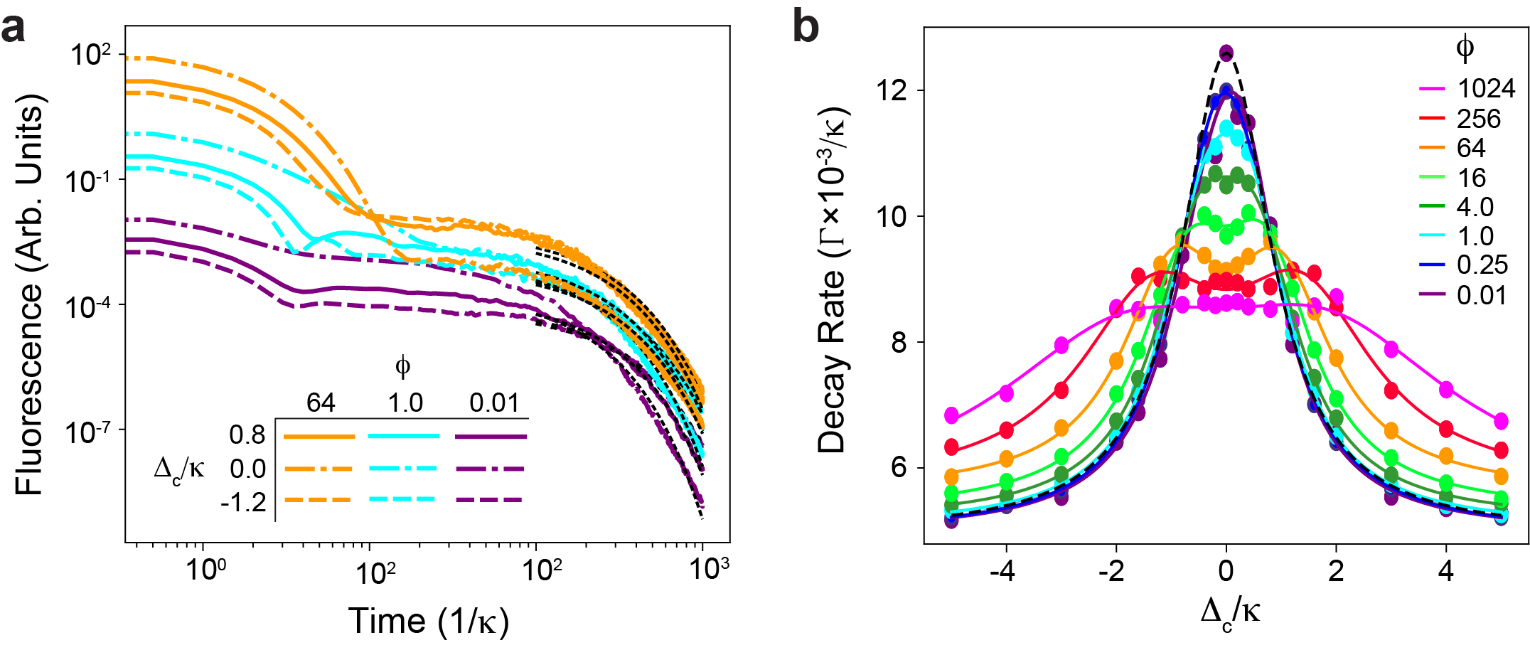
Figure 3: Simulated PLE measurements on cavity-coupled Er ensembles, based on the semiclassical model of the relaxation dynamics given by Eqs. (4) to (6). (a) Nine examples of the disorder-averaged fluorescence $\overline{F(t)}$, defined in Eq. (12), for three different incident photon-flux values ($\phi=|\beta_{\mathrm{in}}|^{2}$) and cavity-laser detuning values $\Delta_{\mathrm{c}}$. The various dotted black lines are exponential fits $c\exp(-\Gamma t)$ to the decay dynamics for $t\gg 1/\kappa$. (b) The spontaneous decay rate relative to the cavity decay rate ($\Gamma/\kappa$) as a function of the cavity-laser detuning ($\Delta_{\mathrm{c}}$) for increasing photon flux values ($\phi$). The solid lines for each flux are double Lorentzian fits to the simulated data. The dashed black line is a single Lorentzian function with FWHM $2\kappa$.

The ratio between the spontaneous decay rate $\Gamma$ and the cavity decay rate $\kappa$ is shown in Figure 3(b). Despite the fact that we approximate the full quantum dynamics with a semiclassical model and ignore the presence of Er ions coupled to the bus waveguide, the spontaneous decay rate qualitatively reproduces the experimental measurements shown in Figure 1(d): At the smallest input flux $\phi=0.01$, the spontaneous decay rate is maximum on resonance, $\Delta_{\mathrm{c}}=0$ and decreases for finite cavity detuning according to a Lorentzian function whose FWHM is given by $2\kappa$, $L(\Delta_{\mathrm{c}},0,\kappa)$ (dashed black curve in Fig. 3(b)). This is in rough agreement with our experimental findings where the Lorentzian lineshape of the Purcell enhanced decay rate is $\approx 35$% wider than the cavity linewidth as determined from reflection scans. At a slightly larger input flux of $\phi=0.25$, the curve of the decay rate shows a flat region around zero detuning, which is consistent with the curve being the sum of two detuned Lorentzian functions. This interpretation also lets us understand the behavior at higher fluxes $\phi\gtrsim 16$, where one sees two distinct local maxima at finite detuning $|\Delta_{\mathrm{c}}|>0$. The separation of these new maxima increases with drive power and ultimately exceeds $2\kappa$. At the same time, the decay rate for a resonant cavity decreases.

To quantify the separation between the two Lorentzian functions, we fit the decay rate to $a[L(\Delta_{\mathrm{c}},\Delta_{+},h_{+})+L(\Delta_{\mathrm{c}},\Delta_{-},h_{-})]+b$. Free parameters are the overall amplitude $a$, the offset $b$, the detunings $\Delta_{\pm}$ of the two peaks, and the corresponding width parameters $h_{\pm}$. These fits are shown by the solid lines in Figure 3(b). The ratio between the maximum decay rate $\Gamma$ at a given input flux $\phi$, $\max_{\Delta_{\mathrm{c}}}(\Gamma|_{\phi})$, and its corresponding value at the smallest input flux $\phi_{\mathrm{min}}$, $\max_{\Delta_{\mathrm{c}}}(\Gamma|_{\phi_{\mathrm{min}}})$, are shown in Figure 4(b) as a function of the rescaled flux $\phi/\phi_{0}$. We find that the semiclassical model agrees with the experimental data for $\phi/\phi_{0}\lesssim 1$. Here, $\phi_{0}$ is the critical flux above which saturation effects start to become relevant. It can be extracted from fits of the integrated fluorescence to the PLE curve (1), $\phi_{0}=1/p_{2}$ (see SI). Moreover, in the same regime $\phi\ll\phi_{0}$, the separation of the corresponding maxima $\Delta_{\pm}$ as a function of $\phi/\phi_{0}$ in the semiclassical model agrees well with the experimental splitting (see SI). Larger deviations between the semiclassical and the experimental data emerge when entering the saturation regime $\phi\gg\phi_{0}$. We attribute this effect to the different values of the inhomogeneous broadening $\Delta_{\mathrm{inh}}$ in the experiment and the simulations: Intuitively, $\Delta_{\mathrm{inh}}$ determines the spectral extent of the ion ensemble and defines an upper bound on the maximum possible splitting $\Delta_{+}-\Delta_{-}$. Due to the smaller value of $\Delta_{\mathrm{inh}}$, these finite size effects of the ion ensemble will manifest themselves more pronouncedly in the simulations.

3.4 Comparison with an effective local model

Given that the initial state of the fluorescence decay, given by Eqs. (7), (10), and (11), is well-described by a product state of independent spins, where collective effects only enter via the self-energy term determining the steady-state cavity field that drives each spin (a relatively weak correction for the experimental parameters), one may wonder if a similarly simple model of independently decaying spins is sufficient to describe the double-peak structure of the fluorescence decay shown in Figures 2 and 3. One might reasonably expect that given the strong inhomogeneous broadening, the spin decay induced by the cavity does not have any significant collective nature, but is instead equivalent to independent decay of each spin. This independent decay would correspond to each spin having a relaxation dissipator, with a Purcell relaxation rate of spin $j$ determined by the cavity density of states at frequency $\delta_{j}$. The total decay rate of spin $j$ is then given by:

$$\gamma_{\mathrm{eff},j}=\gamma+\frac{\kappa g_{j}^{2}}{(\Delta_{\mathrm{c}}-\delta_{j})^{2}+\kappa^{2}/4}~{}.$$ (13)

To keep the fact that every spin feels the same Rabi drive due to the semiclassical part $\overline{a}(t)$ of the cavity field, we add a Rabi drive to each ion and arrive at the following effective model.

$$\frac{\mathrm{d}}{\mathrm{d}t}\hat{\rho} =\sum_{j=1}^{N}\left(-i\left[\hat{H}_{j},\hat{\rho}\right]+\gamma_{\mathrm{eff},j}\mathcal{D}[\hat{\sigma}_{-}^{j}]\hat{\rho}\right)~{},$$ (14)

$$\hat{H}_{j} =\delta_{j}\frac{\hat{\sigma}_{z}^{j}}{2}+g_{j}\left[\overline{a}^{*}\hat{\sigma}_{-}^{j}+\overline{a}\hat{\sigma}_{+}^{j}\right]~{},$$ (15)

$$\frac{\mathrm{d}}{\mathrm{d}t}\overline{a} =-\left(i\Delta_{\mathrm{c}}+\frac{\kappa}{2}\right)\overline{a}~{}.$$ (16)

The corresponding semiclassical equations of motion of the spins are

$$\frac{\mathrm{d}}{\mathrm{d}t}s_{-}^{j} =-\left(i\delta_{j}+\frac{\gamma_{\mathrm{eff,j}}}{2}\right)s_{-}^{j}+ig_{j}\overline{a}s_{z}^{j}~{},$$ (17)

$$\frac{\mathrm{d}}{\mathrm{d}t}s_{z}^{j} =2ig\left[\overline{a}^{*}s_{-}^{j}-\overline{a}(s_{-}^{j})^{*}\right]-\gamma_{\mathrm{eff},j}(1+s_{z}^{j})~{}.$$ (18)

Despite naive intuition suggesting that this non-collective description of cavity-mediated spin decay should be sufficient, we now show that its predictions both qualitatively and quantitatively disagree with the full semiclassical model (which includes potential collective effects) and the experimental observations.

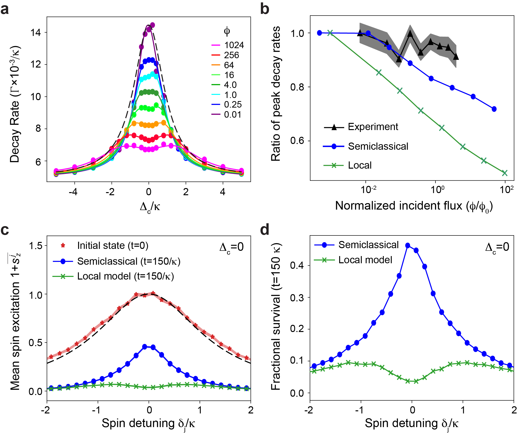
Figure 4: Comparison between the semiclassical model given by Eqs. (4) to (6), and an effective model where each spin experiences only local decay, given by Eqs. (16) to (18). (a) The spontaneous decay rate relative to the cavity decay rate ($\Gamma/\kappa$), as a function of the cavity-laser detuning ($\Delta_{\mathrm{c}}$) for increasing photon flux values ($\phi$) for the effective local model. The black dashed line corresponds to a Lorentzian function of linewidth 2$\kappa$. (b) Maximum decay rate as a function of the incident flux $\phi$ relative to the corresponding value for the smallest incident flux, $\max_{\mathrm{\Delta}_{\mathrm{c}}}(\Gamma)/\max_{\mathrm{\Delta}_{\mathrm{c}}|_{\phi}}(\Gamma|_{\phi_{\mathrm{min}}})$, as a function of the photon flux ($\phi$), normalized to the critical photon flux ($\phi_{0}$) where saturation effects start to occur (see main text). The gray shaded areas indicate the standard deviation of the measurement results. (c) Mean spin excitation $1+\overline{s_{z}^{j}}$ as a function of spin detuning $\delta_{j}$ for the initial state immediately after the pulse (red stars) and at $t=150/\kappa$ after the pulse for the semiclassical model (blue dots) as well as the effective local model (green crosses). The dashed black curve is the theory expression for the mean spin excitation, Eq. (10) with $g_{j}$ replaced by $\overline{g}$. The cavity is resonant with the drive laser, $\Delta_{\mathrm{c}}=0$. (d) Corresponding fractional survival probabilities $[1+\overline{s_{z}^{j}}(t)]/[1+\overline{s_{z}^{j}}(0)]$ as a function of the cavity-laser detuning for the semiclassical and the effective local model. The simulation parameters are the same as in Fig. 3.

To analyze the fluorescence generated by our approximate “local" (i.e. non-collective) model of cavity-induced spin decay, we numerically integrate Eqs. (16) to (18) for $n_{\mathrm{traj}}$ different random disorder configurations, starting from the same initial conditions as in the unmodified semiclassical model given by Eqs. (4) to (6). Since each spin is effectively relaxing into a different auxiliary cavity mode, which has been adiabatically eliminated and led to the Purcell-enhancement term in Eq. (13), we need to modify the definition of the fluorescence signal: The rate at which ion $j$ emits a photon into its associated auxiliary cavity mode at time $t$ is given by $\gamma_{\mathrm{eff},j}[1+s_{z}^{j}(t)]/2$. The fluorescence due to relaxation of the spins can now be calculated by summing up these expressions for all spins. In addition, the decay of the initial cavity field $\overline{a}$ will also generate output photons, such that the total fluorescence in a timestep $\mathrm{d}t$ is

$$\overline{F(t)}=\kappa_{\mathrm{c}}\left[|\overline{a}|^{2}+\sum_{j=1}^{N}\gamma_{\mathrm{eff},j}\frac{1+\overline{s_{z}^{j}(t)}}{2}\mathrm{d}t\right]~{}.$$ (19)

Given this modified definition of $\overline{F(t)}$, we perform the same exponential fits as described in Sec. 3.3. The corresponding results are shown in Figure  4(a).

In comparison with the corresponding results of the semiclassical model, shown in Figure 3(b), and the experimental measurements, shown in Figure 1(d), there is a striking qualitative difference: even though the separation of the two maxima in the decay rate $\Gamma$ increases very similarly as a function of the incident photon flux $\phi$ (see SI), the local model predicts that separation of the maxima is accompanied by a strong suppression of the maximum value of $\Gamma$ as $\phi$ grows. Therefore, the curves at large $\phi$ never extend beyond the Lorentzian function $L(\Delta_{\mathrm{c}},0,\kappa)$ set by the data corresponding to the smallest input flux. In contrast, both the experimental data and the semiclassical model show a much weaker suppression of the maximum value of $\Gamma$ with increasing $\phi$, such that the curves at large input flux are significantly broader than the Lorentzian function shape corresponding to the smallest input flux. This is clearly visible in the comparison between the maximum of the decay rate at a given input flux $\phi$, $\max_{\Delta_{\mathrm{c}}}(\Gamma|_{\phi})$, and the corresponding value at the smallest input flux $\phi_{\mathrm{min}}$, $\max_{\Delta_{\mathrm{c}}}(\Gamma|_{\phi_{\mathrm{min}}})$ in Fig. 4(b). As discussed above, at low input fluxes $\phi/\phi_{0}\lesssim 1$, the semiclassical model and the experimental data agree well within the experimental error bars. The local model, however, deviates strongly from the other two curves. The semiclassical model starts to deviate from the experimental data for $\phi\approx\phi_{0}$, which we attribute to the fact that the numerical simulations use a significantly smaller inhomogeneous broadening $\Delta_{\mathrm{inh}}$ than the experimental setup. At $\phi\approx\phi_{0}$, the splitting $\Delta_{+}-\Delta_{-}$ in the semiclassical simulations becomes comparable to $\Delta_{\mathrm{inh}}$, such that corrections due to the finite extent of the simulated ion ensemble are likely to become relevant. In the experiment, the corresponding corrections would manifest themselves only at much higher input fluxes. Another difference between the local model vs. both the semiclassical model and the experimental data is the behavior of the offset fit parameter $b$ as a function of $\phi/\phi_{0}$: For the effective local model, $b$ decreases monotonically with increasing $\phi/\phi_{0}$, whereas for semiclassical simulations and the experimental data, $b$ is fairly constant or slightly increasing as a function of $\phi/\phi_{0}$.

To better understand why the fluorescence signal predicted by the local model deviates so strongly from the full semiclassical model, it is helpful to consider other observables. In this regard, a striking feature of the full dynamics is that some spins, which are expected to have a large Purcell-enhanced decay rate, actually decay much slower than naively expected, as illustrated in Figures 4(c) and (d). To investigate the average decay of a spin at a given detuning $\delta_{j}$ from the drive laser, we bin the spins of each disorder distribution according to their random detuning $\delta_{j}$. We then calculate the spin excitation $1+s_{z}^{j}$ for all spins and average them within each bin. The distribution of the mean spin excitation of the initial state at time $t_{\mathrm{pulse}}$ is given by the red stars in Figure 4(c) and matches well the theory expression (10) with $g_{j}$ replaced by $\overline{g}$. The shaded regions represent the standard deviation of the mean spin excitation in each bin. As the spins fluoresce, the mean spin excitation decreases. For the effective local model, given by the green crosses in Figure 4(c), the spins that are resonant with the cavity, $\delta_{j}\approx\Delta_{\mathrm{c}}=0$, have the largest decay rate $\gamma_{\mathrm{eff},j}$. This leads to a suppression of spin excitation on resonance at late times, as shown by the fractional survival probability plotted in Figure 4(d). Surprisingly, this naive expectation does not hold for the full semiclassical model. Here, the spins that are resonant with the cavity actually maintain their excitation longer than detuned spins with a seemingly smaller local decay rate, as shown by the blue data points in Figures 4(c) and (d). This striking feature indicates collective effects play an important role in the dynamics. Further, this behavior cannot be understood by simply involving the CIT argument, which relates the structure of the initial state to a renormalized cavity density of states (see SI). Instead, it suggests that the collective decay physics and cavity-mediated spin-spin interactions (both dissipative and coherent) play a crucial role in the dynamics.

4 Conclusion

In this work, we have used an inhomogeneously broaden ensemble of Er ions evanescently coupled to a relatively narrow optical nanocavity to explore optical decay dynamics as a function of laser-cavity detuning and pump power. In order to realize these measurements, we developed a materials-compatible nanofabrication process to greatly improve the device-to-fiber photon collection efficiency. Our resonant PLE measurements reveal an interesting three-fold suppression of the Purcell-enhanced optical lifetime at the highest pump fluence measured when the cavity is resonant with the optical transition. We estimate that the number of ions participating in this effect is roughly 2000 at the highest incident photon flux. We have employed a semiclassical model that captures qualitative aspects of the experimental optical relaxation even with a modest number of $N=61$ ions.

From these simulations, there appear to be rich decay dynamics that happen in the time regime between traditional cavity photon and spin decay processes ($\sim 1/\kappa<t<1/\Gamma$) that are not being accessed in the current experimental configuration. In the future, it would be beneficial to switch to gated operation of single photon detectors that can simultaneously enable higher collection efficiency by removal of a lossy modulator in the collection path and detection of photons earlier in the relaxation process. In addition, there are likely other interesting dynamics that occur as the photons impinge and reflect from the cavity, as has been explored recently in the regime of spectrally narrower but larger ensembles of ions coupled to lower Q cavities[27].

From a modeling perspective, it would be beneficial to optimize the numerical implementation to investigate these effects in larger ensembles that approach the experimental number of ions probed. A much larger simulated ensemble size can enable us to modify other parameters to better emulate experimental conditions: such as increasing the ensemble inhomogeneous linewidth, reducing the cavity-waveguide coupling efficiency $\kappa_{\mathrm{c}}$, and broadening the disorder averaged ion-cavity coupling strength. In doing so, we may be able to reduce potential finite-size effects in the splitting of the peak decay rates as a function of $\phi$ to better match experimental results. On the theory side, an analytical understanding of the emergence of the double-peaked structure in the fluorescence decay rate is desired, and such insights would provide clarity on the origin of the surprising survival of excitations in spins that are resonant with the cavity mode.

Funding The authors acknowledge the Q-NEXT Quantum Center, a U.S. Department of Energy, Office of Science, National Quantum Information Science Research Center, under Award Number DE-FOA-0002253 for support (M. K., C. J., G. D. G., I. M., D. D. A., S. G., A. A. C., A. M. D.). All electron microscopy and device fabrication was performed at the Center for Nanoscale Materials, a U.S. Department of Energy Office of Science User Facility, supported by the U.S. DOE, Office of Basic Energy Sciences, under Contract No. DE-AC02-06CH11357. Additional materials characterization support (M. T. S., S. E. S., and F. J. H.) was provided by the U.S. Department of Energy, Office of Science; Basic Energy Sciences, Materials Sciences, and Engineering Division.

Acknowledgments The authors would like to thank D. Czaplewski, C. S. Miller, and R. Divan for assistance with device fabrication.

Disclosures

“The authors declare no conflicts of interest.”

Supplemental document See Supplementary Information for supporting content.

References

- [1] K. Hammerer, A. S. Sørensen, and E. S. Polzik, “Quantum interface between light and atomic ensembles,” \JournalTitleRev. Mod. Phys. 82, 1041–1093 (2010).
- [2] A. Reiserer and G. Rempe, “Cavity-based quantum networks with single atoms and optical photons,” \JournalTitleRev. Mod. Phys. 87, 1379–1418 (2015).
- [3] E. M. Purcell, H. C. Torrey, and R. V. Pound, “Resonance absorption by nuclear magnetic moments in a solid,” \JournalTitlePhysical Review 69, 37–38 (1946).
- [4] H. Walther, B. T. H. Varcoe, B.-G. Englert, and T. Becker, “Cavity quantum electrodynamics,” \JournalTitleReports on Progress in Physics 69, 1325 (2006).
- [5] E. Jaynes and F. Cummings, “Comparison of quantum and semiclassical radiation theories with application to the beam maser,” \JournalTitleProceedings of the IEEE 51, 89–109 (1963).
- [6] R. H. Dicke, “Coherence in spontaneous radiation processes,” \JournalTitlePhys. Rev. 93, 99–110 (1954).
- [7] M. Gross and S. Haroche, “Superradiance: An essay on the theory of collective spontaneous emission,” \JournalTitlePhysics Reports 93, 301–396 (1982).
- [8] V. V. Temnov and U. Woggon, “Superradiance and subradiance in an inhomogeneously broadened ensemble of two-level systems coupled to a low-$q$ cavity,” \JournalTitlePhysical Review Letters 95, 243602– (2005).
- [9] M. A. Norcia, R. J. Lewis-Swan, J. R. K. Cline, et al., “Cavity-mediated collective spin-exchange interactions in a strontium superradiant laser,” \JournalTitleScience 361, 259–262 (2018).
- [10] Z. Kurucz, J. H. Wesenberg, and K. Mølmer, “Spectroscopic properties of inhomogeneously broadened spin ensembles in a cavity,” \JournalTitlePhysical Review A 83, 053852– (2011).
- [11] B. Julsgaard and K. Mølmer, “Dynamical evolution of an inverted spin ensemble in a cavity: Inhomogeneous broadening as a stabilizing mechanism,” \JournalTitlePhys. Rev. A 86, 063810 (2012).
- [12] B. Julsgaard and K. Mølmer, “Fundamental limitations in spin-ensemble quantum memories for cavity fields,” \JournalTitlePhys. Rev. A 88, 062324 (2013).
- [13] M. Blaha, A. Johnson, A. Rauschenbeutel, and J. Volz, “Beyond the tavis-cummings model: Revisiting cavity qed with ensembles of quantum emitters,” \JournalTitlePhysical Review A 105, 013719– (2022).
- [14] J. D. Thompson, T. G. Tiecke, N. P. de Leon, et al., “Coupling a single trapped atom to a nanoscale optical cavity,” \JournalTitleScience 340, 1202–1205 (2013).
- [15] J. Gallego, W. Alt, T. Macha, et al., “Strong purcell effect on a neutral atom trapped in an open fiber cavity,” \JournalTitlePhys. Rev. Lett. 121, 173603 (2018).
- [16] A. Kumar, A. Suleymanzade, M. Stone, et al., “Quantum-enabled millimetre wave to optical transduction using neutral atoms,” \JournalTitleNature 615, 614–619 (2023).
- [17] H. Mabuchi, J. Ye, and H. J. Kimble, “Full observation of single-atom dynamics in cavity qed,” \JournalTitleApplied Physics B 68, 1095–1108 (1999).
- [18] A. Goban, C.-L. Hung, J. D. Hood, et al., “Superradiance for atoms trapped along a photonic crystal waveguide,” \JournalTitlePhys. Rev. Lett. 115, 063601 (2015).
- [19] D. E. Chang, J. S. Douglas, A. González-Tudela, et al., “Colloquium: Quantum matter built from nanoscopic lattices of atoms and photons,” \JournalTitleReviews of Modern Physics 90, 031002– (2018).
- [20] M. Mirhosseini, E. Kim, X. Zhang, et al., “Cavity quantum electrodynamics with atom-like mirrors,” \JournalTitleNature 569, 692–697 (2019).
- [21] J. M. Kindem, A. Ruskuc, J. G. Bartholomew, et al., “Control and single-shot readout of an ion embedded in a nanophotonic cavity,” \JournalTitleNature 580, 201–204 (2020).
- [22] M. Raha, S. Chen, C. M. Phenicie, et al., “Optical quantum nondemolition measurement of a single rare earth ion qubit,” \JournalTitleNature Communications 11, 1605 (2020).
- [23] S. Chen, M. Raha, C. M. Phenicie, et al., “Parallel single-shot measurement and coherent control of solid-state spins below the diffraction limit,” \JournalTitleScience 370, 592–595 (2020).
- [24] S. Ourari, Ł. Dusanowski, S. P. Horvath, et al., “Indistinguishable telecom band photons from a single er ion in the solid state,” \JournalTitleNature 620, 977–981 (2023).
- [25] T. Xie, J. Rochman, J. G. Bartholomew, et al., “Characterization of for microwave to optical transduction,” \JournalTitlePhys. Rev. B 104, 054111 (2021).
- [26] J. Rochman, T. Xie, J. G. Bartholomew, et al., “Microwave-to-optical transduction with erbium ions coupled to planar photonic and superconducting resonators,” \JournalTitleNat. Commun. 14, 1–9 (2023).
- [27] M. Lei, R. Fukumori, J. Rochman, et al., “Many-body cavity quantum electrodynamics with driven inhomogeneous emitters,” \JournalTitleNature 617, 271–276 (2023).
- [28] A. M. Dibos, M. T. Solomon, S. E. Sullivan, et al., “Purcell enhancement of erbium ions in tio2 on silicon nanocavities,” \JournalTitleNano Letters 22, 6530–6536 (2022).
- [29] C. Ji, M. T. Solomon, G. D. Grant, et al., “Nanocavity-mediated purcell enhancement of er in tio2 thin films grown via atomic layer deposition,” (2023).
- [30] M. K. Singh, A. Prakash, G. Wolfowicz, et al., “Epitaxial Er-doped Y2O3 on silicon for quantum coherent devices,” \JournalTitleAPL Mater. 8, 031111 (2020).
- [31] K. Shin, I. Gray, G. Marcaud, et al., “Er-doped anatase TiO2 thin films on LaAlO3 (001) for quantum interconnects (QuICs),” \JournalTitleAppl. Phys. Lett. 121, 081902 (2022).
- [32] M. K. Singh, G. Wolfowicz, J. Wen, et al., “Development of a scalable quantum memory platform – materials science of erbium-doped tio2 thin films on silicon,” (2022).
- [33] S. M. Meenehan, J. D. Cohen, S. Gröblacher, et al., “Silicon optomechanical crystal resonator at millikelvin temperatures,” \JournalTitlePhys. Rev. A 90, 011803 (2014).
- [34] A. M. Dibos, M. Raha, C. M. Phenicie, and J. D. Thompson, “Atomic source of single photons in the telecom band,” \JournalTitlePhysical Review Letters 120, 243601– (2018).
- [35] C. M. Phenicie, P. Stevenson, S. Welinski, et al., “Narrow optical line widths in erbium implanted in tio2,” \JournalTitleNano Letters 19, 8928–8933 (2019).
- [36] L. Weiss, A. Gritsch, B. Merkel, and A. Reiserer, “Erbium dopants in nanophotonic silicon waveguides,” \JournalTitleOptica 8, 40–41 (2021).
- [37] D. F. Walls and G. J. Milburn, Quantum Optics (Springer-Verlag Berlin Heidelberg, 2008).