Results on Elastic Cross Sections in Proton–Proton Collisions at $\sqrt{s}=510$ GeV with the STAR Detector at RHIC

Abstract

We report results on an elastic cross section measurement in proton–proton collisions at a center-of-mass energy $\sqrt{s}=510$ GeV, obtained with the Roman Pot setup of the STAR experiment at the Relativistic Heavy Ion Collider (RHIC). The elastic differential cross section is measured in the four-momentum transfer squared range $0.23\leq-t\leq 0.67$ GeV². We find that a constant slope $B$ does not fit the data in the aforementioned $t$ range, and we obtain a much better fit using a second-order polynomial for $B(t)$. The $t$ dependence of $B$ is determined using six subintervals of $t$ in the STAR measured $t$ range, and is in good agreement with the phenomenological models. The measured elastic differential cross section $\mathrm{d}\sigma/\mathrm{dt}$ agrees well with the results obtained at $\sqrt{s}=546$ GeV for proton–antiproton collisions by the UA4 experiment. We also determine that the integrated elastic cross section within the STAR $t$-range is $\sigma^{\mathrm{fid}}_{\mathrm{el}}=462.1\pm 0.9(\mathrm{stat.})\pm 1.1(\mathrm{syst.})\pm 11.6(\mathrm{scale})$ $\mu\mathrm{b}$.

1 Introduction

Most of the proton–proton ($pp$) elastic scattering cross-section measurements are in the four-momentum transfer squared $t$ range where perturbative QCD (pQCD) cannot be applied. Here, $t=(p_{\mathrm{in}}-p_{\mathrm{out}})^{2}$, where $p_{\mathrm{in}}$, $p_{\mathrm{out}}$ represent the four-momenta of the incoming and outgoing proton, respectively. Unlike the case for pQCD, where the QCD Lagrangian is used to calculate the scattering amplitudes, the calculations in the low $t$ range are done in the Regge framework [1, 2, 3, 4], where the amplitudes are evaluated in the framework of scattering matrix (S-Matrix) theory. Those scattering amplitudes ${\cal A}(s,t)$ depend on the square of center-of-mass energy $s$, and $t$. Regge theory provides rigorous constraints on the properties of the scattering amplitudes ${\cal A}(s,t)$.

In the $t$ range of this measurement, $0.23\leq-t\leq 0.67$ GeV², the elastic cross section $d\sigma/dt$ is described by the hadronic term of the scattering amplitude ${\cal A}(s,t)$ with an exponential dependence on $t$: $d\sigma/dt=|{\cal A}(s,t)|^{2}=A\cdot e^{-B(t)\,|t|}$. Although the theory allows for the exponential slope $B$ to depend on $t$, the data show that at a given $\sqrt{s}$ the slope is approximately constant for small $|t|$ but changes at large $|t|$. For example, there is a well-known change in slope at $|t|\approx 0.13$ GeV² as discussed in [5].

At $\sqrt{s}\gtrsim 10$ GeV energies, depending on $\sqrt{s}$, the elastic scattering contributes 18 – 28% to the total cross section. Hence, it is important to measure it at every available $\sqrt{s}$. Each new data set provides additional information, which is then used in the tuning of phenomenological models of elastic scattering. If measured at low enough $t$, the elastic cross section allows a determination of the total cross section. For these reasons, elastic scattering has typically been measured at all particle accelerator facilities.

This paper reports the results on $pp$ elastic scattering at $\sqrt{s}=510$ GeV, which is below those most recently measured at the LHC with center-of-mass energies $2.76\leq\sqrt{s}\leq 13$ TeV [6, 7, 8, 9, 10, 11]. It is above the $\sqrt{s}$ range of the Intersecting Storage Rings (ISR) measurements carried out about 50 years ago at $\sqrt{s}=62.4$ GeV [12, 13] and a recent STAR measurement [14] of $pp$ elastic scattering in a lower $|t|$ range at $\sqrt{s}=200$ GeV. The $p\bar{p}$ elastic scattering was measured at the $S\!\mbox{$p\bar{p}$}S$ collider at $\sqrt{s}=546$ and $630$ GeV [15, 16, 17] and at the Tevatron at 1.8 TeV and 1.96 TeV [18, 19, 20].

2 The Experiment

The results presented here are obtained with the setup described in [14], whose main features are described below. For these measurements at $\sqrt{s}=510$ GeV, the STAR experiment [21] was upgraded with the Roman Pot (RP) system used previously by the PP2PP experiment [22]. The location of the RPs, top and side views, and the coordinate system are shown schematically in Fig. 1. Each RP station contains four Silicon (Si) strip detectors and a trigger scintillation counter. The elastic scattering is determined in the STAR coordinate system, where the $z$-axis is in the direction of the clockwise-going RHIC beam, the $y$-axis is pointing up and the $x$-axis completes the right-handed coordinate system whose origin is at the interaction point (IP).

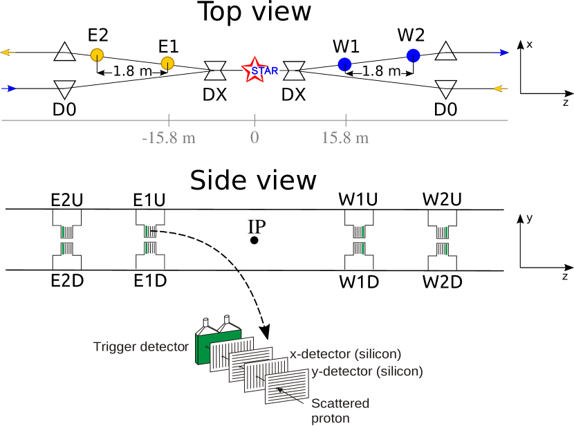
Figure 1: The layout of the RP setup at STAR (not to scale) for measuring forward protons. Top $(x,z)$ and side $(y,z)$ views are shown. Two sets of RPs, labeled (W1, W2) and (E1, E2) were installed between the DX and D0 magnets, at 15.8 m and 17.6 m, on either side of the IP. The detector package has transverse size $5\times 8\;\mathrm{cm}^{2}$ and a depth 3.5 cm. The Si sensor is $400\;\mu\mathrm{m}$ thick, while the trigger scintillator is 5 mm thick. The strips in the Si detectors are $\approx 100\;\mu$m wide. Two dipole magnets, DX and D0, which bend the beams into and out of the IP, are also shown.

The DX magnet, the RHIC-lattice dipole magnet closest to the IP, and the detectors in the two sets of RPs enable the measurement of the momentum vector of the scattered protons at the detection point. Using that information the scattering angle at the IP is determined. Because of the symmetry of the RHIC rings, the fields in the DX magnets on both sides of the IP are identical at the $10^{-3}$ level. Therefore, the bending angles of the magnets are also the same.

The data for the results reported here were acquired in the RHIC 2017 run during the period with a special accelerator optics with $\beta^{*}\approx 8$ m, (where $\beta^{*}$ is the $\beta$-function value at the collision point), which reduced beam angular divergence, as compared to the standard running conditions. Luminosity monitors were calibrated using Van der Meer scans [23]. The range of instantaneous luminosity was $6\>\mbox{to}\>13\cdot 10^{31}\>\mbox{cm}^{-2}\mbox{s}^{-1}$. The associated systematic uncertainty on the luminosity measurement is 2.2%.

The RPs were moved as close to the beam as possible; the closest position of the first readout strip was about 20 mm, which corresponds to a minimum $|t|$ of about 0.16 $\mbox{GeV}^{2}$. The aperture of the DX magnet and the following beam pipe structure determined a maximum achievable value of $|t|\approx 1.1\,\mbox{GeV}^{2}$, corresponding to a scattering angle of $\theta\approx 4~{}\mbox{mrad}$. In this paper, we analyze the elastic scattering in the region of uniform geometrical acceptance in the range $0.23\leq-t\leq 0.67$ GeV². This allows us to minimize the background due to beam halo and scattering on the apertures.

There are about $28\cdot 10^{6}$ triggered events for the integrated luminosity of $6.91\;\mbox{nb}^{-1}$. They satisfy the elastic scattering trigger condition:

$$\mathbf{(EU\land WD)\lor(ED\land WU)},$$ (1)

where EU denotes a valid PMT signal in at least one of the PMTs of the EU1 or EU2 trigger counters. Similarly, ED, WU and WD denote valid PMT signals in the other trigger counters, as shown in Fig. 1.

3 Clustering, Track Reconstruction and Alignment

Track reconstruction in the Si detectors is a multi-step process. Initially, clustering is used to determine the position of the proton trajectory in a Si plane. Then, the reconstruction of a point (PT) in a RP is performed. Finally, the scattering angles are reconstructed and the $t$ value is determined.

3.1 Clustering

First, to make sure that the deposited energy in a Si strip is above the noise, the energy measured in that strip is required to be larger than $5\sigma_{\mathrm{ped}}$, where $\sigma_{\mathrm{ped}}$ is the average pedestal width of the 126 channels in one readout SVXIIE chip [24].

Second, a clustering procedure for each Si plane is performed following Ref. [14]. However, in this analysis, there is a minimum energy cut, which depends on the cluster length, i.e., the number of consecutive strips in the cluster. Clusters longer than 5 strips are excluded. These cluster energy and cluster size cuts, determined in a data-driven way, are used to suppress background. The signal-to-noise ratio is about $20:\!1$, as measured by the Most Probable Value of the Landau $dE/dx$ distribution for a cluster size of one strip and is found to be larger for larger clusters.

Third, matching of the clusters between planes measuring the same coordinate is performed to reconstruct a PT’s $(x,y)$ coordinates in a given RP. The clusters are considered matched if the distance between them is less than 300 $\mu$m. In case a cluster is found in only one of the planes for a given coordinate, that coordinate is used only if there are matched clusters in the other coordinate. These PTs are used to reconstruct the scattering angles.

3.2 Track and Scattering Angle

Two points reconstructed on the same side of the IP, one in each RP, define a track. The scattering angles $(\theta_{x},\theta_{y})$, in the $(x,z)$ and in the $(y,z)$, plane of that track are calculated using those two PTs:

$$\theta_{x}=\frac{X_{\mathrm{RP2}}-X_{\mathrm{RP1}}}{Z_{\mathrm{RP2}}-Z_{\mathrm{RP1}}},\mathrm{\hskip 28.45274pt}\theta_{y}=\frac{Y_{\mathrm{RP2}}-Y_{\mathrm{RP1}}}{Z_{\mathrm{RP2}}-Z_{\mathrm{RP1}}},$$ (2)

where RP1 and RP2 denote near and far RP stations with respect to the IP. The coordinates $(X_{\mathrm{RP}},Y_{\mathrm{RP}})$ are with respect to the nominal beam trajectory. The $Z_{\mathrm{RP}}$ is the $z$-position of the RP with respect to the IP.

About $70\%$ of the events had one and only one PT per RP on the upper (lower) East or West side of the IP. Alignment is performed for each run in the analysis using the procedure described in Ref. [14]. The resulting run-by-run corrections to the positions of the strips are applied before the reconstruction of the scattering angles. As such, the alignment offsets are obtained in the system of coordinates where the two protons are elastically scattered, a collinear elastic scattering geometry.

4 Data Analysis

In this section, we describe the flow of the data analysis. The scattering angles $\theta_{x}$ and $\theta_{y}$ are calculated from the points reconstructed in the Si detectors, as described above. Then cuts are applied to select elastic scattering events.

4.1 Analysis Selection Criteria

The various selection criteria for choosing elastic events are described below in the order as they are applied in the analysis:

Elastic event topology (ET): Only events with a combination of reconstructed points in the RPs consistent with elastic scattering are accepted. Namely, the combinations with the lower East detector in coincidence with the upper West detector, arm EDWU, or the upper East detector in coincidence with the lower West detector, arm EUWD, satisfy the elastic event topology due to momentum conservation.

Four Roman Pot (4RP) event data sample: Only events with at least one reconstructed point per RP on the East and on the West are kept.

Four PT (4PT) events: 4RP events with one and only one PT per RP and no reconstructed points in the Si in the other arm. Using 4PT events the scattering angles ($\theta_{x},\theta_{y})$ on each side of the IP are calculated as indicated in Eq. 2.

Collinear (COL) events: The $\theta_{W}$ and $\theta_{E}$ are the reconstructed polar scattering angles on the West and East sides of the IP, respectively. Because of momentum conservation, collinearity in $\theta_{W}$, $\theta_{E}$ is required. Hence, $\Delta\theta=\theta_{W}-\theta_{E}$ is expected to be zero. Consequently, we select the events for which $|\Delta\theta|\leq 3\sigma_{\Delta\theta}$, where $\sigma_{\Delta\theta}=50$ $\mu\mbox{rad}$ is the Gaussian width of the collinearity distribution, consistent with the beam angular divergence. The collinearity condition also requires that the distance between the two projected tracks in $x$ and $y$ at $z=0$ be within a radius of $3\sigma$ of the Gaussian width of their distributions. In Fig. 2, we show the collinearity distribution $\Delta\theta_{y}$ vs $\Delta\theta_{x}$, where $\Delta\theta_{x}=\theta_{x}^{W}-\theta_{x}^{E}$ and $\Delta\theta_{y}=\theta_{y}^{W}-\theta_{y}^{E}$. Here, the $\theta_{x}^{W},\theta_{x}^{E},\theta_{y}^{W},\theta_{y}^{E}$ are scattering angles reconstructed on the West and East sides of the IP, using the measured coordinates at the RP and after the fiducial volume cut. A clear peak of elastic events is seen. The contours of $2\sigma_{\Delta\theta}$ and $3\sigma_{\Delta\theta}$ are also shown.

Fiducial volume (GEO) cut: After the elastic event candidates are chosen based on collinearity, one more set of cuts in a fiducial volume $(\phi,|t|)$, where $\phi$ is the azimuthal angle of the proton scattering, is needed to remove the remaining background. To stay away from the beam halo, a minimum $|t|$ corresponding to $12\sigma$ of the beam size is required, well outside of the beam envelope. Hence, a coincidence arising from the beam halo from the two beams is not expected. To stay away from the apertures, additional cuts on the maximum $|t|$ and on the $\phi$-range are also required. The chosen $\phi$, $|t|$ ranges are $78^{\circ}\leq|\phi|\leq 102^{\circ}$ and $0.23\leq-t\leq 0.67$ GeV², respectively. The fiducial cuts are shown in Fig. 3. These cuts are chosen based on the simulation, which is described in Sec. 5.1.

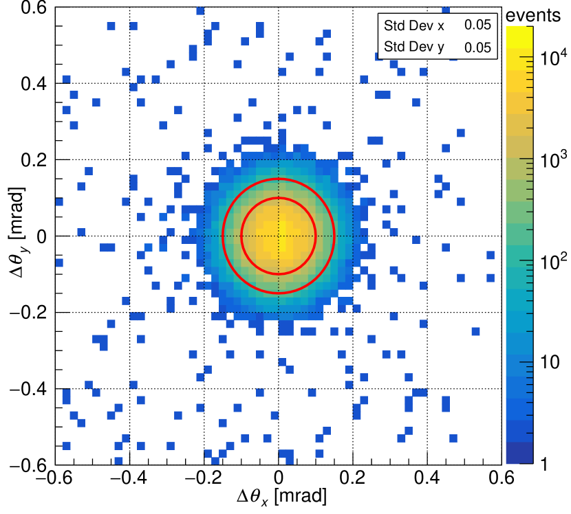
Figure 2: The collinearity of the data sample for accepted ET events is shown. It is defined as the differences $\Delta\theta_{x}$ and $\Delta\theta_{y}$ between the scattering angles $\theta_{x}$, $\theta_{y}$ reconstructed on the East and West side of the IP. Contours of $2\sigma_{\Delta\theta}$ and $3\sigma_{\Delta\theta}$, where $\sigma_{\Delta\theta}\approx\sigma_{\Delta\theta_{x}}\approx\sigma_{\Delta\theta_{y}}\approx 50~{}\mu\mbox{rad}$, are shown as red circles.

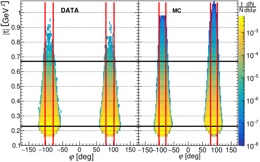
Figure 3: Four-momentum transfer $|t|$ vs $\phi$ distributions for data and MC for 4PT collinear events. The two elastic combinations of tracks between East and West, EUWD and EDWU, are shown. The GEO cuts in $t$ and $\phi$ are shown as black and red lines, respectively.

4.2 The $t$ Reconstruction

The scattering angles $\theta_{x}$ and $\theta_{y}$ are determined by fitting a straight line using 4PT events and $\chi^{2}$ minimization. Given the beam momentum $p$ and small scattering angles $\theta_{x}$ and $\theta_{y}$, the $t$-value is calculated using:

$$t=(p_{\mathrm{in}}-p_{\mathrm{out}})^{2}\approx-p^{2}\theta^{2}=-p^{2}\cdot(\theta_{x}^{2}+\theta_{y}^{2}).$$ (3)

The resolution in $t$ is dominated by the beam angular divergence, which is about $30~{}\mu\mbox{rad}$ for both $\theta_{x}$ and $\theta_{y}$, as given by the beam emittance and by the $\beta$-function value at the collision point ($\beta^{*}$). The detector spacial resolution is a small fraction of the $t$ resolution. The measured standard deviations of the angular distributions of $(\Delta\theta_{x},\Delta\theta_{y})$ are $\thicksim 50~{}\mu\mbox{rad}$, as shown in Fig. 2. They are consistent with the estimate of the beam angular divergence and position reconstruction resolution in the Si detectors.

5 Efficiency Corrections

The efficiency correction has two terms: 1) efficiency which accounts for the limited geometrical acceptance and point reconstruction efficiency in a RP; 2) the trigger efficiency. The former has two components: a MC component, which accounts mainly for geometrical acceptance, and a data-driven $t$-dependent point reconstruction efficiency within the geometrical acceptance. The trigger efficiency is obtained from the data using Zero Bias (ZB) triggers, which are events triggered on beam crossings only.

We introduce a correction function $C(t)$, which relates the number of reconstructed elastic events $N_{\mathrm{rec}}^{\mathrm{DATA}}(t)$ obtained from data to the number of events produced at the vertex $N_{\mathrm{cor}}^{\mathrm{DATA}}(t)$:

$$N_{\mathrm{cor}}^{\mathrm{DATA}}(t)=N_{\mathrm{rec}}^{\mathrm{DATA}}(t)\cdot C(t).$$ (4)

The corrections from which $C(t)$ is obtained are discussed in the following sections.

5.1 Geometrical Acceptance and Track Reconstruction Efficiency

To determine the $t$-dependent geometrical acceptance of the RP detector system, a GEANT4-based [25] simulation is used. The simulation includes a detailed description of the DX magnet including all limiting apertures, the RP details, and the Si readout behavior. The latter includes known hardware problems, such as the two non-working (out of 80) SVX readout chips and one non-working (out of 32) Si planes. The two non-working SVXs were mostly outside of the geometrical acceptance. The energy deposited by final state particles in the Si detectors is digitized and added to the electronic noise obtained from the pedestal runs. To reproduce the impact of background, the MC generated events are embedded in the ZB data sample. This is done by combining the list of clusters from the ZB events with the list of simulated clusters. The overlaying clusters are merged and their positions are recalculated. After the embedding, a standard PT reconstruction, including cluster matching, is done the same way as in the real data. The $pp$ elastic scattering is generated using uniform distributions in $t$ and $\phi$ ranges of $0.1\leq|t|\leq 1.5~{}\mbox{GeV}^{2}$ and $-\pi\leq\phi<\pi$, respectively. As a result, the geometrical acceptance of the detector is obtained as the main contribution to the efficiency correction function defined as:

$$\varepsilon_{\mathrm{MC}}(t)=\frac{N^{\mathrm{MC}}_{\mathrm{rec}}(t)}{N^{\mathrm{MC}}_{\mathrm{gen}}(t)}\ or\ C_{\mathrm{MC}}(t)=\frac{1}{\varepsilon_{\mathrm{MC}}(t)},$$ (5)

where $N^{\mathrm{MC}}_{\mathrm{gen}}(t)$ and $N^{\mathrm{MC}}_{\mathrm{rec}}(t)$ are the true and reconstructed distributions obtained as functions of generated and reconstructed $t$, respectively.

That purely geometrical acceptance factor, based on an angular acceptance $\Delta\phi=\pm 12^{\circ}$, is in first order $C_{\mathrm{MC}}=360^{\circ}/24^{\circ}=15$. Furthermore, to account for the fact that the MC events are generated with flat distributions, the data are reweighted event by event using the FMO model [26]. The systematic effect of the reweighting procedure is estimated in Sec. 5.4.

The efficiency of point reconstruction for each RP is estimated using the data sub-sample containing only events with one reconstructed point in each of the three RPs, not including the RP under the test. A track is reconstructed using those three points. The track has to pass the GEO filters to ensure that it crossed the geometrical acceptance of each RP, and then is projected to the RP under test. If the distance $D$ between the projected position of the track and the reconstructed point in that RP is less than $1.5$ mm and the reconstructed 4PT event satisfied the criteria for an elastic event, that RP is considered efficient and the count is added to the $N_{\mathrm{pass}}$ sample. If the event does not satisfy those criteria, the count is added to the $N_{\mathrm{fail}}$ sample. The PT reconstruction efficiency is then obtained as the ratio of the number of tracks crossing a given RP with the reconstructed PT found in this RP to the number of all tracks crossing the RP, and measured as a function of reconstructed $t$:

$$\varepsilon^{\mathrm{PT}}_{\mathrm{RP}}(t)=\frac{N_{\mathrm{pass}}(t)}{N_{\mathrm{pass}}(t)+N_{\mathrm{fail}}(t)}.$$ (6)

More than 99% of the events projected into a RP satisfy the $D\leq 1.5$ mm cut. Hence, this cut does not affect the event reconstruction efficiency. This criterion is only used to select possible 4PT event candidates, for which collinearity (COL) and geometrical acceptance (GEO) criteria for an elastic event are checked.

The four $\varepsilon^{\mathrm{PT}}_{\mathrm{RP}}(t)$ efficiencies are not independent. In addition to the four separate cases where events are lost due to either no point or more than one point in the tested RP, there is a common case for all four RP’s. This occurs when a 4PT event made of single reconstructed points does not pass the standard elastic selection imposed on 4PT events, resulting in a $\varepsilon^{\mathrm{COL}}_{\mathrm{RP}}(t)$ for each RP. Since we find this value to be constant for all RPs, that common factor $\varepsilon_{\mathrm{COL}}(t)\approx 0.98$ is used as the overall correction factor.

The efficiency for each arm $\varepsilon_{\mathrm{arm}}(t)$, EUWD or EDWU combinations of the RPs, is then obtained as the product of the above five independent efficiencies in that arm $\varepsilon_{\mathrm{arm}}(t)=\varepsilon_{\mathrm{4PT}}(t)\cdot\varepsilon_{\mathrm{COL}}(t)$, where $\varepsilon_{\mathrm{4PT}}(t)$ is a product of the four efficiencies of finding a point (PT) in each RP before a collinearity cut is applied. The same procedure as for the data is also used for the MC embedded sample. The difference between the two is at the level of a few percent per RP, within its geometrical acceptance, and is interpreted as the effect of unknown inefficiencies present in the data and not included in the MC simulation (e.g., caused mainly by either no point or more than one point reconstructed in a single RP). It should be noted that no point in most cases means that too large a cluster was observed which is then not classified as a reconstructed point. To account for that, a correction function $C_{\mathrm{T}}(t)$ to tune $\varepsilon_{\mathrm{MC}}$ is used:

$$C_{\mathrm{T}}(t)=\frac{\varepsilon_{\mathrm{arm}}^{\mathrm{MC-EMBD}}(t)}{\varepsilon_{\mathrm{arm}}^{\mathrm{DATA}}(t)},$$ (7)

where $\varepsilon_{\mathrm{arm}}^{\mathrm{MC-EMBD}}$ and $\varepsilon_{\mathrm{arm}}^{\mathrm{DATA}}$ are the elastic event reconstruction efficiencies obtained from the MC embedded sample and the data, respectively.

The systematic uncertainty on $\varepsilon^{\mathrm{PT}}_{\mathrm{RP}}(t)$ is estimated by varying the collinearity cut for 3PT events used to calculate the RP efficiency from the nominal $3\sigma$ by $\pm 1\sigma$.

5.2 Trigger Efficiency

The elastic event data stream contains only events triggered by the coincidence of valid PMT signals consistent with the trigger condition in Eq. 1. The trigger efficiency is defined as the ratio of the number of events reconstructed with the silicon detectors satisfying the pattern in Eq. 1 and confirmed by the PMT trigger ($N_{\mathrm{trig}}^{\mathrm{rec}}$), over the number of all reconstructed events ($N^{\mathrm{rec}}_{\mathrm{all}}$) fulfilling the trigger condition:

$$\varepsilon_{\mathrm{trig}}(t)=\frac{N^{\mathrm{rec}}_{\mathrm{trig}}(t)}{N^{\mathrm{rec}}_{\mathrm{all}}(t)}.$$ (8)

The trigger efficiency is calculated using the ZB data sample by comparing the trigger bit with the combination of PMT signals in a given event. A constant value $\varepsilon_{\mathrm{trig}}=0.986^{\scriptstyle+0.008}_{\scriptstyle-0.015}$ is used, as obtained by integration over the acceptance of this measurement. The quoted statistical uncertainty of the trigger efficiency is treated as an independent source of the overall normalization uncertainty and is added in quadrature to the other normalization uncertainties.

5.3 The Correction Function

The full correction function used to correct the number of reconstructed 4PT elastic events $N_{\mathrm{rec}}(t)$ is calculated as:

$$C(t)=\frac{C_{\mathrm{MC}}(t)\cdot C_{\mathrm{T}}(t)}{\varepsilon_{\mathrm{trig}}(t)},$$ (9)

where $C_{\mathrm{MC}}(t)=1/\varepsilon_{\mathrm{MC}}(t)$. Consequently, the differential distribution $(dN/dt)^{\mathrm{DATA}}$ obtained from data is corrected using a “bin-by-bin” method applying the above correction factors:

$$\bigg{(}\frac{dN}{dt}\bigg{)}^{\mathrm{DATA}}_{\mathrm{cor}}=C(t)\cdot\bigg{(}\frac{dN}{dt}\bigg{)}^{\mathrm{DATA}}_{\mathrm{rec}}.$$ (10)

The values of $C(t)$ for each arm are shown in Fig. 4. One can see that although there is some variation, the factors $\mathrm{C}(t)$ are relatively uniform and are within the range $17.6<\mathrm{C}(t)<18.8$ in the $t$ interval of the measurement. The small modulations observed are due to known individual Si detector plane response behaviors.

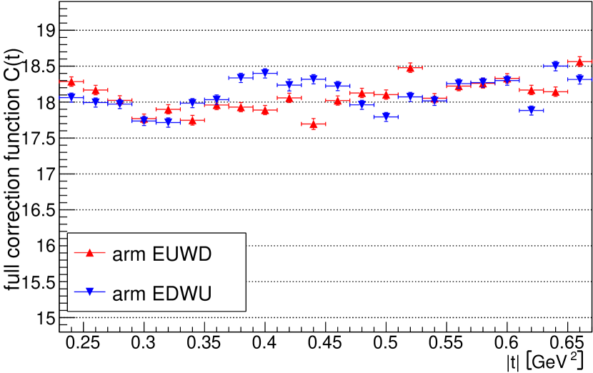
Figure 4: The full correction function $C(t)$ applied to the data is shown separately for each detector arm. The horizontal error bars indicate the bin size.

5.4 MC Weighting Function Correction

Since the MC is generated with a flat distribution in $t$ while the data has an exponential dependence on $t$, a reweighting of the $dN/dt$ distributions is necessary. A reweighting function based on the FMO model [26] is used. The systematic uncertainty due to the use of that model is obtained by multiplying the model weighting function by $e^{\pm t}$ and reweighting the $dN/dt$ distributions event by event. The factor $e^{\pm t}$ corresponds to the uncertainty on the slope $B(t)$. The resulting differences in the differential cross section $d\sigma/dt$ are the estimated uncertainties on the differential cross section due to the use of the reweighting function. They are a fraction of the statistical uncertainty and are listed in Table 1.

6 Beam Tilt

Since the elastic scattering is reconstructed in the RP reference system, additional corrections are needed because of a possible non-zero initial colliding-beam angle or beam tilt in that reference frame. Such a beam tilt affects the $t$ scale of the measurement. Note that the offset due to the $(x,y)$ position of the beam at the IP, being a parallel shift, does not change the reconstructed scattering angles $\theta_{x},\theta_{y}$, which are the result of fitting a straight line to the 4PT events.

The beam-tilt angle results in offsets $\tau_{x}$ and $\tau_{y}$ of the reconstructed $\theta_{x}$ and $\theta_{y}$ angles and consequently leads to an offset $\Delta t$ in the calculated $t$-value. In lowest order, where terms proportional to $\tau_{x}^{2}$ and $\tau_{y}^{2}$ are neglected, it is given by:

$$\Delta t\simeq 2p^{2}(\theta_{x}\tau_{x}+\theta_{y}\tau_{y}).$$ (11)

In the absence of beam tilt, the ratio of the differential cross sections in two arms $R(t)=(d\sigma/dt)_{\mathrm{EUWD}}/(d\sigma/dt)_{\mathrm{EDWU}}$ is expected to be one. The tilt angle $\tau_{x}$ is estimated by forcing the mean value $\langle\theta_{x}\rangle$ of the reconstructed $dN/d\theta_{x}$ to be zero as expected from an elastic event topology, resulting in $\tau_{x}=75\pm 2\,\mu\mathrm{rad}$, which is confirmed by the MC simulation.

In order to find the $\tau_{\mathrm{y}}$ we use $\ln{R(|t|)}$, which is a linear function of the difference between the $B(|t|)$ slopes of the two arms. Hence, linear fits to $\ln{R(|t|)}$ are performed in the range $0.23\leq-t\leq 0.67$ GeV² by iterating the values of $\tau_{y}$ while $\tau_{x}$ is set to zero. When that ratio becomes flat the residual slope is $0.00\pm 0.05$. The corresponding systematic uncertainty due to $\tau_{y}$ is obtained by finding the $\tau_{y}$ for which the slope of the fitted line is one standard deviation from zero, namely $\pm 0.05$. This procedure yields $\tau_{y}\approx 20\pm 5\,\mu\mathrm{rad}$. These values of $(\tau_{x},\tau_{y})$ are then added to the reconstructed values of $(\theta_{x},\theta_{y})$.

After the above $(\tau_{x},\tau_{y})$ corrections, the cross sections $d\sigma/dt$ measured separately for the two arms EUWD and EDWU, agree not only in shape but also in normalization to within 2% level, which is consistent with statistical fluctuations. The uncertainty on the beam tilt, to which the $\tau_{x}$ systematic uncertainty contribution is negligible, is propagated to the systematic uncertainty on the cross section measurements and is shown in Table 1. It is found to be very small compared to the statistical error.

7 Background

The background estimate is shown in Fig. 5, where the collinearity distributions for reconstructed data and reconstructed MC samples are compared after the GEO cut. In addition to beam halo coincidences and secondary interactions in front of the RPs, the data contains possible physics background sources such as central diffraction and coincidence of two protons from a single diffraction dissociation. In Fig. 5, background in the GEANT4-based simulation is also presented. The latter includes background from protons interacting with the material in front of the RPs, such as the beam pipe, magnet structure, the RF shield inside the DX-D0 chamber, etc. Since the collinearity distributions for MC and for data are normalized to unity, the vertical axis (P_EVT) in Fig. 5 is the probability per event.

For the background estimate, a second-order polynomial is fitted to collinearity distributions of the data with the exclusion of the $\pm 5\sigma$ central region. The resulting polynomial is then extrapolated to the central region ($\pm 3\sigma$) of the collinearity distribution, which is the region where the elastic events are used to obtain the cross sections. The background level, compared to the signal within that central phase space is found to be $(0.020\pm 0.002)\%$, which is negligible and therefore not corrected. The background analysis is repeated in four $t$ regions. The background slightly increases with $|t|$, but is still negligible at the level of 0.1% at $|t|\approx 0.6$ GeV².

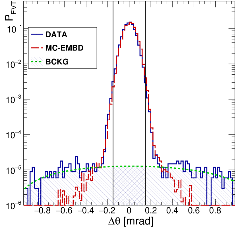
Figure 5: Collinearity, $\Delta\theta=\theta_{\mathrm{W}}-\theta_{\mathrm{E}}$, for both simulation (MC-EMBD) and data (DATA) are shown. The vertical axis (P_EVT) is the probability per event. Both samples are displayed after the fiducial volume (GEO) cut. Estimated background (BCKG), hatched area, and background remaining after collinearity cut, cross-hatched area, are also shown. For the latter, the fraction compared to the signal within the collinearity cut is $0.020\pm 0.002\%$.

8 Results

The final result for $d\sigma/dt$ in the $t$ range of this measurement, $0.23\leq|t|\leq 0.67$ GeV², is obtained as a weighted average of $d\sigma/dt$ obtained from each of the two arms of the experiment, where the weights are calculated using statistical errors of the individual points. In Fig. 6 we plot our results and compare them with those from the UA4 experiment for $p\bar{p}$ at $\sqrt{s}=546$ GeV. We find a very good agreement between the two measurements as shown in the bottom panel of Fig. 6, where the ratio is close to one within the experimental uncertainties. The systematic shift one observes in the ratio to the UA4 data could be due to a difference in UA4 luminosity normalization, since the associated systematic is reported to be different, which is 5% for UA4 [15] for lower $|t|$ values, and 10% [16] for larger $|t|$ values. The statistical and systematic uncertainties on the STAR data points are smaller than the plotted data points, which with their associated uncertainties are presented in Table 1 and in the HEPData database [27]. The uncertainties on the ratio are dominated by the uncertainties of the UA4 data.

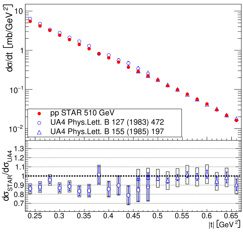
Figure 6: Top panel: The $pp$ elastic differential cross section $d\sigma/dt$ from this experiment compared with the results of the UA4 experiment. Bottom panel: the ratio of the two measurements (STAR/UA4). Uncertainties are statistical only and are smaller than the symbols for the STAR data. The rectangles in the bottom panel show the total systematic uncertainty (STAR + UA4) on the ratio. The vertical scale uncertainty of 2.5% on the STAR data points, and of 5% or 10% (see text) for UA4 data points are not shown here.

In the $t$ range of the present measurement, the differential cross section is described by an exponential function $d\sigma_{\mathrm{el}}/dt=A\cdot\exp{[-B(t)|t|]}$, where $A$ is a normalization constant and $B(t)$ is well approximated by a second order polynomial:

$$B(t)=B_{0}+B_{1}\cdot|t|+B_{2}\cdot|t|^{2}.$$ (12)

The $t$ region $|t|<0.23$ GeV² is excluded from the analysis due to the significant background contribution from beam halo protons and uncertainty related to detector edge effects. We find that the fit with the $B(t)=\mathrm{const}$ has a small probability ($\approx 0.001$) and that the quadratic dependence $B(t)$ has a much higher probability of $0.202$. Consequently, we present our result using an exponential fit with $B(t)$ as a second-order polynomial to the measured $d\sigma_{\mathrm{el}}/dt$. The fit results are shown in Fig. 7 and Table 2.

The integrated elastic scattering cross section, $\sigma^{\mathrm{fid}}_{\mathrm{el}}$, within the STAR $t$ acceptance of $0.23\leq|t|\leq 0.67~{}\mbox{GeV}^{2}$ is $\sigma^{\mathrm{fid}}_{\mathrm{el}}=462.1\pm 0.9(\mathrm{stat.})\pm 1.1(\mathrm{syst.})\pm 11.6(\mathrm{scale})$ $\mu\mathrm{b}$.

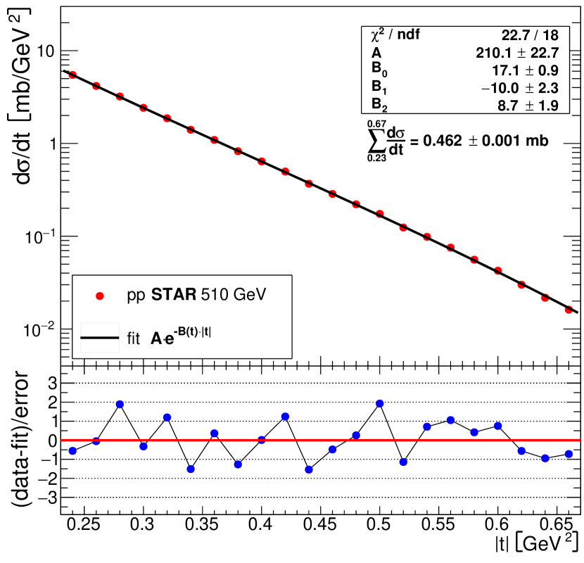
Figure 7: Top panel: The $pp$ elastic differential cross section $d\sigma/dt$ fitted with an exponential $Ae^{-B(t)|t|}$ with $B(t)$ as in Eq. 12. Bottom panel: Residuals (Data - Fit)/Error. Uncertainties on the data points are smaller than the symbol size.

As described earlier, the estimated background contribution due to particle interactions with the material in front of the RPs and diffractive physics processes within the geometrical acceptance used for this analysis is negligible. Table 2 contains our results and uncertainty estimates on the exponential fit parameters listed in the left column: the normalization constant $A$, the slope parameter $B(t)$ and the elastic cross section within STAR’s $t$ range $\sigma^{\mathrm{fid}}_{\mathrm{el}}$. The systematic uncertainty on the fitted parameters $A$, $B_{0}$, $B_{1}$, and $B_{2}$ is obtained as half of the difference between the fit parameters in the two arms. The second to last column of Table 2 lists the total uncertainty, which is calculated by adding the individual uncertainties in quadrature. For the cross section measurements, the largest systematic uncertainty is the scale uncertainty due to the luminosity determination, which is 2.2%. The total scale uncertainty, which includes trigger efficiency uncertainty of 1.2% is 2.5%. This scale uncertainty does not affect the value of the slope parameters $B(t)$, but introduces a corresponding systematic uncertainty to the cross sections as listed in Table 2.

Table 1: The measured $pp$ elastic differential cross sections $d\sigma/dt$, with results from the detector arms averaged for the final data sample, as shown in Fig. 7. The cross section and the center of each $t$ interval, $\boldsymbol{t_{\mathrm{cent}}}$, are given in [$\mu$b/GeV²] and [GeV²], respectively. The statistical, systematic, and full uncertainties are also listed. The scale uncertainty of 2.5% is not included in the full error.

$t_{\mathrm{cent}}$	d$\sigma$/dt	err. stat.	err. sys.	err. full
0.24	5472.8	$\pm 23.5$	$\pm 11.3$	$\pm 26.1$
0.26	4167.4	$\pm 19.6$	$\pm 8.9$	$\pm 21.5$
0.28	3206.8	$\pm 16.6$	$\pm 5.9$	$\pm 17.6$
0.30	2419.9	$\pm 13.9$	$\pm 6.0$	$\pm 15.1$
0.32	1868.5	$\pm 12.0$	$\pm 4.8$	$\pm 12.9$
0.34	1404.4	$\pm 10.2$	$\pm 4.1$	$\pm 11.0$
0.36	1091.6	$\pm 8.9$	$\pm 2.9$	$\pm 9.4$
0.38	824.9	$\pm 7.7$	$\pm 1.8$	$\pm 7.9$
0.40	640.2	$\pm 6.7$	$\pm 1.4$	$\pm 6.8$
0.42	498.0	$\pm 5.9$	$\pm 2.1$	$\pm 6.3$
0.44	368.2	$\pm 5.0$	$\pm 1.4$	$\pm 5.2$
0.46	285.5	$\pm 4.4$	$\pm 0.7$	$\pm 4.4$
0.48	220.7	$\pm 3.9$	$\pm 0.6$	$\pm 3.9$
0.50	174.1	$\pm 3.4$	$\pm 0.5$	$\pm 3.4$
0.52	124.1	$\pm 2.9$	$\pm 1.5$	$\pm 3.2$
0.54	98.4	$\pm 2.6$	$\pm 0.6$	$\pm 2.6$
0.56	75.4	$\pm 2.3$	$\pm 0.5$	$\pm 2.3$
0.58	55.8	$\pm 1.9$	$\pm 0.5$	$\pm 2.0$
0.60	42.5	$\pm 1.7$	$\pm 0.5$	$\pm 1.8$
0.62	30.0	$\pm 1.4$	$\pm 0.5$	$\pm 1.5$
0.64	21.7	$\pm 1.2$	$\pm 0.4$	$\pm 1.3$
0.66	16.2	$\pm 1.1$	$\pm 0.4$	$\pm 1.1$

Table 2: Results of the exponential function fit (Eq. 12) to the elastic differential cross section data as well as the integrated fiducial cross section are listed. Also listed are the corresponding values of the statistical and systematic uncertainties. The scale (luminosity and trigger efficiency) uncertainty of 2.5% applicable to the fit parameter A and fiducial cross section $\boldsymbol{\sigma^{\mathrm{fid}}_{\mathrm{fid}}}$ is not included in the full error.

name	units	Value	err. stat.	err. sys.	full
$\boldsymbol{A}$	mb/GeV2	210.1	$\pm 22.7$	$\pm 11.6$	$\pm 24.1$
$\boldsymbol{B_{0}}$	GeV-2	17.1	$\pm 0.9$	$\pm 0.3$	$\pm 0.9$
$\boldsymbol{B_{1}}$	GeV-4	$-10.0$	$\pm 2.3$	$\pm 0.7$	$\pm 2.4$
$\boldsymbol{B_{2}}$	GeV-6	8.7	$\pm 1.9$	$\pm 0.6$	$\pm 2.0$
$\boldsymbol{\sigma^{\mathrm{fid}}_{\mathrm{el}}}$	$\mu$b	462.1	$\pm 0.9$	$\pm 1.1$	$\pm 1.4$

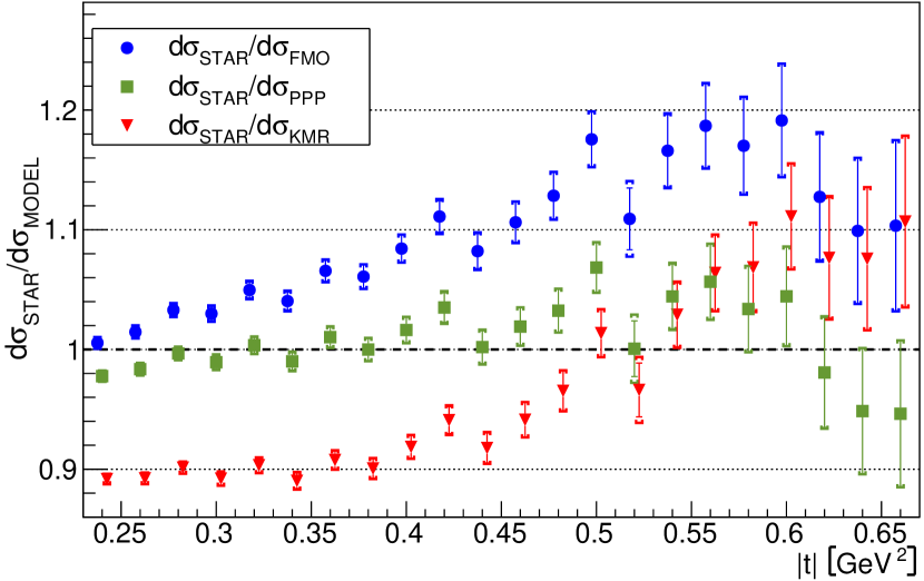
Figure 8: Comparison of the STAR $pp$ differential cross section results with FMO [26], KMR [28] and PPP [29] models. The ratio of the STAR measured cross section to the model predictions is shown as a function of $t$. The square brackets, where seen, indicate the systematic uncertainty of the STAR data points; otherwise, they are smaller than the symbols themselves.

In Fig. 8 we compare our $\mathrm{d}\sigma/\mathrm{d}t$ result with three model predictions. The first model (FMO) has a maximum Odderon [30] amplitude as described in [26], the second is a two-channel eikonal model (KMR) [28] and the third utilizes a three component Pomeron and an Odderon (PPP) [29]. We find our result in good agreement with those models, although the agreement is generally better for $|t|<0.40\;\mathrm{GeV}^{2}$ than for $|t|$ above that value.

In order to characterize the shape, we fit a $B=\mbox{const.}$ slope in six sub-intervals of our $t$ range as shown in Fig. 9. There is a good qualitative agreement with the three models shown; there is a minimum in $B(t)$ at $-t\approx 0.40\>\mathrm{GeV}^{2}$.

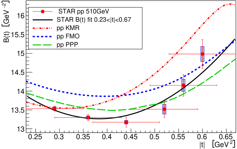
Figure 9: Comparison of the STAR $pp$ result in six $t$ sub-intervals with three models: FMO [26], KMR [28] and PPP [29]. The black line is fit to the full data set as described in Eq. 12. The horizontal size of the error bars indicate the $t$ range where $B=\mathrm{const.}$ was fitted. The vertical size of the shaded rectangles indicates the systematic uncertainty of the STAR data points.

9 Summary

We present the STAR experiment’s measurement of the elastic differential cross sections for $pp$ scattering at $\sqrt{s}=510$ GeV as a function of $t$ in the range $0.23\leq|t|\leq 0.67$ GeV². In that range, the elastic differential cross section is well described by the exponential function $e^{-B(t)|t|}$, where $B(t)$ is a second-order polynomial whose parameters are shown in Fig. 7 and Table 2. We also present the elastic cross section integrated within the STAR fiducial $t$ range to be $\sigma^{\mathrm{fid}}_{\mathrm{el}}=462.1\pm 0.9(\mathrm{stat.})\pm 1.1(\mathrm{syst.})\pm 11.6(\mathrm{scale})$ $\mu\mathrm{b}$. We compare $d\sigma_{el}/dt$, in the measured $t$ range, with the results obtained in $p\bar{p}$ collisions at $\sqrt{s}=546$ GeV and find that they are in good agreement. The $\mbox{d}\sigma/\mbox{d}t$ and the shape of $B(t)$, also obtained using six sub-intervals in our $t$ range, are in good agreement with the phenomenological models.

References

- [1] T. Regge, Introduction to complex orbital momenta, Nuovo Cim. 14 (1959) 951. doi:10.1007/BF02728177.
- [2] P. D. B. Collins, An Introduction to Regge Theory and High-Energy Physics, Cambridge University Press, 2009. doi:10.1017/CBO9780511897603.
- [3] V. Barone, E. Predazzi, High-Energy Particle Diffraction, Springer, 2002. doi:10.1007/978-3-662-04724-8.
- [4] S. Donnachie, H. G. Dosch, O. Nachtmann, P. Landshoff, Pomeron physics and QCD, Vol. 19, Cambridge University Press, 2004.
- [5] G. Matthiae, Proton and anti-proton cross-sections at high-energies, Rept. Prog. Phys. 57 (1994) 743–790. doi:10.1088/0034-4885/57/8/001.
- [6] TOTEM Collaboration, G. Antchev, et al., First measurement of elastic, inelastic and total cross-section at TeV by TOTEM and overview of cross-section data at LHC energies, Eur. Phys. J. C 79 (2) (2019) 103. arXiv:1712.06153, doi:10.1140/epjc/s10052-019-6567-0.
- [7] TOTEM Collaboration, G. Antchev, et al., Luminosity-independent measurements of total, elastic and inelastic cross-sections at TeV, EPL 101 (2) (2013) 21004. doi:10.1209/0295-5075/101/21004.
- [8] TOTEM Collaboration, G. Antchev, et al., Measurement of elastic pp scattering at TeV in the Coulomb–nuclear interference region: determination of the -parameter and the total cross-section, Eur. Phys. J. C 76 (12) (2016) 661. arXiv:1610.00603, doi:10.1140/epjc/s10052-016-4399-8.
- [9] TOTEM Collaboration, G. Antchev, et al., Elastic differential cross-section at and implications on the existence of a colourless C-odd three-gluon compound state, Eur. Phys. J. C 80 (2) (2020) 91. arXiv:1812.08610, doi:10.1140/epjc/s10052-020-7654-y.
- [10] ATLAS Collaboration, G. Aad, et al., Measurement of the total cross section from elastic scattering in pp collisions at TeV with the ATLAS detector, Nucl. Phys. B 889 (2014) 486–548. arXiv:1408.5778, doi:10.1016/j.nuclphysb.2014.10.019.
- [11] ATLAS Collaboration, M. Aaboud, et al., Measurement of the total cross section from elastic scattering in collisions at TeV with the ATLAS detector, Phys. Lett. B 761 (2016) 158–178. arXiv:1607.06605, doi:10.1016/j.physletb.2016.08.020.
- [12] CERN-Pisa-Rome-Stony Brook Collaboration, U. Amaldi, et al., New Measurements of Proton Proton Total Cross-Section at the CERN Intersecting Storage Rings, Phys. Lett. B 62 (1976) 460–466. doi:10.1016/0370-2693(76)90685-7.
- [13] A. Breakstone, et al., A Measurement of and Elastic Scattering in the Dip Region at -GeV, Phys. Rev. Lett. 54 (1985) 2180. doi:10.1103/PhysRevLett.54.2180.
- [14] STAR Collaboration, J. Adam, et al., Results on total and elastic cross sections in proton–proton collisions at = 200 GeV, Phys. Lett. B 808 (2020) 135663. arXiv:2003.12136, doi:10.1016/j.physletb.2020.135663.
- [15] UA4 Collaboration, R. Battiston, et al., Proton - Anti-proton Elastic Scattering at Four Momentum Transfer Up to 0.5-GeV**2 at the CERN SPS Collider, Phys. Lett. B 127 (1983) 472. doi:10.1016/0370-2693(83)90296-4.
- [16] UA4 Collaboration, M. Bozzo, et al., Elastic Scattering at the CERN SPS Collider Up to a Four Momentum Transfer of 1.55-GeV**2, Phys. Lett. B 155 (1985) 197–202. doi:10.1016/0370-2693(85)90985-2.
- [17] UA4 Collaboration, D. Bernard, et al., Large T Elastic Scattering at the CERN SPS Collider at -GeV, Phys. Lett. B 171 (1986) 142–144. doi:10.1016/0370-2693(86)91014-2.
- [18] E710 Collaboration, N. A. Amos, et al., Measurement of , the Ratio of the Real to Imaginary Part of the Forward Elastic Scattering Amplitude, at = 1.8-TeV, Phys. Rev. Lett. 68 (1992) 2433–2436. doi:10.1103/PhysRevLett.68.2433.
- [19] CDF Collaboration, F. Abe, et al., Measurement of small angle elastic scattering at GeV and 1800 GeV, Phys. Rev. D 50 (1994) 5518–5534. doi:10.1103/PhysRevD.50.5518.
- [20] D0 Collaboration, V. M. Abazov, et al., Measurement of the differential cross section in elastic scattering at TeV, Phys. Rev. D 86 (2012) 012009. arXiv:1206.0687, doi:10.1103/PhysRevD.86.012009.
- [21] STAR Collaboration, K. H. Ackermann, et al., STAR detector overview, Nucl. Instrum. Meth. A 499 (2003) 624–632. doi:10.1016/S0168-9002(02)01960-5.
- [22] PP2PP Collaboration, S. Bultmann, et al., The PP2PP experiment at RHIC: Silicon detectors installed in Roman Pots for forward proton detection close to the beam, Nucl. Instrum. Meth. A 535 (2004) 415–420. doi:10.1016/j.nima.2004.07.162.
- [23] S. van der Meer, Calibration of the Effective Beam Height in the ISR, Tech. Rep. CERN-ISR-PO-68-31 (1968).
- [24] T. Zimmerman, M. Sarraj, R. Yarema, I. Kipnis, S. Kleinfelder, L. Luo, O. Milgrome, The SVX2 readout chip, IEEE Trans. Nucl. Sci. 42 (1995) 803–807. doi:10.1109/23.467787.
- [25] GEANT4 Collaboration, S. Agostinelli, et al., GEANT4–a simulation toolkit, Nucl. Instrum. Meth. A 506 (2003) 250–303. doi:10.1016/S0168-9002(03)01368-8.
- [26] E. Martynov, B. Nicolescu, Odderon effects in the differential cross-sections at Tevatron and LHC energies, Eur. Phys. J. C 79 (6) (2019) 461. arXiv:1808.08580, doi:10.1140/epjc/s10052-019-6954-6.
- [27] HEPData Webpage, https://www.hepdata.net/.
- [28] V. A. Khoze, A. D. Martin, M. G. Ryskin, Elastic and diffractive scattering at the LHC, Phys. Lett. B 784 (2018) 192–198. arXiv:1806.05970, doi:10.1016/j.physletb.2018.07.054.
- [29] V. A. Petrov, E. Predazzi, A. Prokudin, Coulomb interference in high-energy pp and anti-p p scattering, Eur. Phys. J. C 28 (2003) 525–533. arXiv:hep-ph/0206012, doi:10.1140/epjc/s2003-01191-7.
- [30] L. Lukaszuk, B. Nicolescu, A Possible interpretation of rising total cross-sections, Lett. Nuovo Cim. 8 (1973) 405–413. doi:10.1007/BF02824484.