Adaptive Output-Feedback Model Predictive Control
of Hammerstein Systems with Unknown Linear Dynamics

Abstract

This paper considers model predictive control of Hammerstein systems, where the linear dynamics are a priori unknown and the input nonlinearity is known. Predictive cost adaptive control (PCAC) is applied to this system using recursive least squares for online, closed-loop system identification with optimization over a receding horizon performed by quadratic programming (QP). In order to account for the input nonlinearity, the input matrix is defined to be control dependent, and the optimization is performed iteratively. This technique is applied to output stabilization of a chain of integrators with unknown dynamics under control saturation and deadzone input nonlinearity.

I Introduction

By performing optimization over a future horizon, model predictive control (MPC) provides the means for controlling systems with state and control constraints [1, 2, 3]. In many applications, however, an accurate model of the controlled system is not available. In this case, data-driven MPC uses a model of the system based on data collected either prior to or during closed-loop operation [4, 5, 6, 7].

The present paper considers output-feedback control of a special class of nonlinear systems, namely, Hammerstein systems, where the dynamics are linear but the control input is subjected to a static nonlinearity, such as control-magnitude saturation [8]. In particular, we assume that the linear dynamics of the plant are a priori unknown, whereas the input nonlinearity is known. These assumptions are realistic in practice when the plant dynamics are subject to unknown changes, but the control hardware is designed and tested separately from the plant.

The novelty of the present paper is to combine predictive cost adaptive control (PCAC) with an iterative receding-horizon optimization technique based on a control-dependent model. PCAC is based on recursive least squares (RLS) for online, closed-loop system identification with optimization [9, 10] over a receding horizon performed by quadratic programming (QP) [11, 12]. As shown in [13], when the online, closed-loop system identification is performed in the presence of harmonic disturbances, the resulting identified model correctly predicts the frequency, amplitude, and phase of the future response, thereby facilitating the ability of MPC to perform disturbance rejection.

The present paper accounts for the input nonlinearity by using a control-dependent model that replaces the input matrix $B$ with the control-dependent matrix $B\sigma(u)/u,$ where $\sigma$ is the input nonlinearity. This technique is used in [14] to compensate for input nonlinearities arising in positive real plants. In the present paper, this technique accounts for the presence of the nonlinearity within the iteration process. In the case where $\sigma$ is a magnitude-saturation function, this technique accounts for the saturation without the need to apply a post-optimization saturation. In the present paper, $B\sigma(u)/u$ is handled through iteration of the receding-horizon optimization, which is performed using QP [15, 1, 16, 17]. Together, these techniques comprise PCAC with an iterative control-dependent coefficient (ICD-PCAC).

ICD-PCAC is demonstrated numerically by means of the well-known chain of integrators example, which has been extensively investigated under full-state feedback [18, 19] and, more recently, under output feedback [20].

The contents of the paper are as follows. Section II presents problem formulation. Section III describes online identification using RLS with variable-rate forgetting, and Section IV presents the input-output model and its block observable canonical form. Section V states the output-feedback MPC problem, and Section VI presents ICD-PCAC for solving the MPC problem. Section VII presents a stopping criterion and warm starting modification for reducing the computational burden of ICD-PCAC. Section VIII provides numerical examples with a chain of integrators dynamics subject to input nonlinearity. Finally, Section IX presents conclusions and future research.

The following notation is used throughout the paper. Let $x_{(i)}$ denote the $i$th component of $x\in{\mathbb{R}}^{n}.$ The symmetric matrix $P\in{\mathbb{R}}^{n\times n}$ is positive semidefinite (resp., positive definite) if all of its eigenvalues are nonnegative (resp., positive).

II Problem Formulation

Consider the continuous-time system

$$\dot{x}(t) =Ax(t)+B\sigma(u(t))+D_{1}d(t),$$ (1)

$$y(t) =Cx(t),$$ (2)

where, for all $t\in[0,\infty)$, $x(t)\in{\mathbb{R}}^{n}$ is the state, $y(t)\in{\mathbb{R}}^{p}$ is the output, $u(t)\in{\mathbb{R}}^{m}$ is the control, $\sigma\colon{\mathbb{R}}^{m}\to{\mathbb{R}}^{m}$ is the known input nonlinearity such that

$$\sigma(0)=0,$$ (3)

and $d(t)\in{\mathbb{R}}^{q}$ is the unknown harmonic or constant disturbance, and $A,B,D_{1},C$ are unknown real matrices of appropriate sizes. For a harmonic disturbance, $d\colon[0,\infty)\to{\mathbb{R}}^{q}$ is given by

$$d(t)=\sum_{i=1}^{n_{d}}d_{{\rm c},i}\cos\omega_{{\rm dis},i}t+d_{{\rm s},i}\sin\omega_{{\rm dis},i}t,$$ (4)

where $n_{d}\geq 1$, and, for all $i\in\{1,\ldots,n_{d}\},$ $\omega_{{\rm dis},i}>0$ is a disturbance frequency, and the vectors $d_{{\rm c},i}\in{\mathbb{R}}^{q}$ and $d_{{\rm s},i}\in{\mathbb{R}}^{q}$ determine the amplitudes and phases of the components of the disturbance. The output $y(t)\in{\mathbb{R}}^{p}$ is sampled and corrupted by discrete-time sensor noise to produce the measurement $y_{k}\in{\mathbb{R}}^{p}$, which, for all $k\geq 0,$ is given by

$$y_{k}\triangleq y(kT_{\rm s})+v_{k},$$ (5)

where $T_{\rm s}>0$ is the sample time, and $v_{k}\in{\mathbb{R}}^{p}$ is the sensor noise.

The objective is to design an adaptive MPC algorithm such that, for all $x_{0}\in{\mathbb{R}}^{n}$, $\lim_{k\to\infty}y_{k}=0$.

III Online identification

Let $\hat{n}\geq 1$ and, for all $k\geq 0,$ let $F_{1,k},\ldots,F_{\hat{n},k}\in{\mathbb{R}}^{p\times p}$ and $G_{1,k},\ldots,G_{\hat{n},k}\in{\mathbb{R}}^{p\times m}$ be the coefficient matrices to be estimated using RLS. Furthermore, let $\hat{y}_{k}\in{\mathbb{R}}^{p}$ be an estimate of $y_{k}$ defined by

$$\hat{y}_{k}\triangleq-\sum_{i=1}^{\hat{n}}F_{i,k}y_{k-i}+\sum_{i=1}^{\hat{n}}{G}_{i,k}\sigma(u_{k-i}),$$ (6)

where

$$y_{-\hat{n}}=\cdots=y_{-1}=0,$$ (7)

$$u_{-\hat{n}}=\cdots=u_{-1}=0.$$ (8)

Using the identity ${\rm vec}(XY)=(Y^{\rm T}\otimes I){\rm vec}X,$ it follows from (6) that, for all $k\geq 0,$

$$\hat{y}_{k}=\phi_{k}\theta_{k},$$ (9)

where

$$\theta_{k} \triangleq{\rm vec}\begin{bmatrix}F_{1,k}&\cdots&\mspace{-10.0mu}F_{\hat{n},k}&\mspace{-10.0mu}G_{1,k}&\cdots&G_{\hat{n},k}\end{bmatrix}\in{\mathbb{R}}^{\hat{n}p(m+p)},$$ (10)

$$\phi_{k} \triangleq\begin{bmatrix}-y_{k-1}^{\rm T}&\mspace{-5.0mu}\cdots&-y_{k-\hat{n}}^{\rm T}&\sigma(u_{k-1})^{\rm T}&\mspace{-5.0mu}\cdots&\sigma(u_{k-\hat{n}})^{\rm T}\end{bmatrix}$$

$$\quad\otimes I_{p}\in{\mathbb{R}}^{p\times\hat{n}p(m+p)}.$$ (11)

To determine the update equations for $\theta_{k}$, for all $k\geq 0$, define $e_{k}\colon{\mathbb{R}}^{\hat{n}p(m+p)}\to{\mathbb{R}}^{p}$ by

$$e_{k}(\bar{\theta})\triangleq y_{k}-\phi_{k}\bar{\theta},$$ (12)

where $\bar{\theta}\in{\mathbb{R}}^{\hat{n}p(m+p)}.$ Using (9), the identification error at each step $k\geq 0$ is defined by

$$e_{k}(\theta_{k})=y_{k}-\hat{y}_{k}.$$ (13)

For all $k\geq 0$, the RLS cumulative cost $J_{k}\colon{\mathbb{R}}^{\hat{n}p(m+p)}\to[0,\infty)$ is defined by [9]

$$J_{k}(\bar{\theta})\triangleq\sum_{i=0}^{k}\frac{\rho_{i}}{\rho_{k}}e_{i}^{\rm T}(\bar{\theta})e_{i}(\bar{\theta})+\frac{1}{\rho_{k}}(\bar{\theta}-\theta_{0})^{\rm T}\Psi_{0}^{-1}(\bar{\theta}-\theta_{0}),$$ (14)

where $\Psi_{0}\in{\mathbb{R}}^{\hat{n}p(m+p)\times\hat{n}p(m+p)}$ is positive definite, $\theta_{0}\in{\mathbb{R}}^{\hat{n}p(m+p)}$ is the initial estimate of the coefficient vector, and, for all $i\geq 0,$

$$\rho_{i}\triangleq\prod_{j=0}^{i}\lambda_{j}^{-1}.$$ (15)

For all $j\geq 0$, the parameter $\lambda_{j}\in(0,1]$ is the forgetting factor defined by $\lambda_{j}\triangleq\beta_{j}^{-1}$, where

$$\beta_{j}\triangleq\begin{cases}1,&j<\tau_{\rm d},\\ 1+\zeta g(e_{j-\tau_{\rm d}}(\theta_{j-\tau_{\rm d}}),\ldots,e_{j}(\theta_{j}))\\ \quad\cdot\textbf{1}\big{(}g(e_{j-\tau_{\rm d}}(\theta_{j-\tau_{\rm d}}),\ldots,e_{j}(\theta_{j}))\big{)},&j\geq\tau_{\rm d},\end{cases}$$

and $\tau_{\rm d}>p$, $\zeta>0$, $\textbf{1}\colon{\mathbb{R}}\to\{0,1\}$ is the unit step function, and $g$ is a function of past RLS identification errors.

To determine $g$ when $p=1$, let $\tau_{\rm n}\in[p,\tau_{\rm d})$, and let $\sigma_{k,\tau_{\rm d}}^{2}$ and $\sigma_{k,\tau_{\rm n}}^{2}$ be the variances of past RLS prediction-error sequences $\{e_{k-\tau_{\rm d}}(\theta_{k-\tau_{\rm d}}),\ldots,e_{k}(\theta_{k})\}$ and $\{e_{k-\tau_{\rm n}}(\theta_{k-\tau_{\rm n}}),\ldots,e_{k}(\theta_{k})\}$, respectively. In this case, $g\colon{\mathbb{R}}^{p}\times\cdots\times{\mathbb{R}}^{p}$ is defined by

$$g(e_{k-\tau_{\rm d}}(\theta_{k-\tau_{\rm d}}),\ldots,e_{k}(\theta_{k}))\triangleq\sqrt{\frac{\sigma_{k,\tau_{\rm n}}^{2}}{\sigma_{k,\tau_{\rm d}}^{2}}}-\sqrt{F_{\tau_{\rm n},\tau_{\rm d}}^{\rm inv}(1-\alpha)},$$ (16)

where $\alpha\in(0,1]$ is the significance level, and $F^{\rm inv}_{\tau_{\rm n},\tau_{\rm d}}(x)$ is the inverse cumulative distribution function of the F-distribution with degrees of freedom $\tau_{\rm n}$ and $\tau_{\rm d}.$ Note that (16) enables forgetting when $\sigma_{\tau_{\rm n}}^{2}$ is statistically larger than $\sigma_{\tau_{\rm d}}^{2}.$ Moreover, larger values of the significance level $\alpha$ cause the level of forgetting to be more sensitive to changes in the ratio of $\sigma_{\tau_{\rm n}}^{2}$ to $\sigma_{\tau_{\rm d}}^{2}$.

When $p>1,$ instead of variances $\sigma_{k,\tau_{\rm d}}$ and $\sigma_{k,\tau_{\rm n}}$, we consider covariance matrices $\Sigma_{k,\tau_{\rm d}}$ and $\Sigma_{k,\tau_{\rm n}}$, and thus the product $\Sigma_{k,\tau_{\rm n}}\Sigma_{k,\tau_{\rm d}}^{-1}$ replaces the ratio $\sigma_{k,\tau_{\rm n}}^{2}/\sigma_{k,\tau_{\rm d}}^{2}$. In this case, $g\colon{\mathbb{R}}^{p}\times\cdots\times{\mathbb{R}}^{p}$ is defined by

$$g(e_{k-\tau_{\rm d}}(\theta_{k-\tau_{\rm d}}),\ldots,e_{k}(\theta_{k})) \triangleq\sqrt{\frac{\tau_{\rm n}}{c\tau_{\rm d}}{\rm tr}\big{(}\Sigma_{k,\tau_{\rm n}}\Sigma_{k,\tau_{\rm d}}^{-1}\big{)}}$$

$$\quad-\sqrt{F^{\rm inv}_{p\tau_{\rm n},b}(1-\alpha)},$$ (17)

where

$$a\triangleq\frac{(\tau_{\rm n}+\tau_{\rm d}-p-1)(\tau_{\rm d}-1)}{(\tau_{\rm d}-p-3)(\tau_{\rm d}-p)},$$ (18)

$$b\triangleq 4+\frac{p\tau_{\rm n}+2}{a-1},\quad c\triangleq\frac{p\tau_{\rm n}(b-2)}{b(\tau_{\rm d}-p-1)}.$$ (19)

Finally, for all $k\geq 0$, the unique global minimizer of $J_{k}$ is given by [9]

$$\theta_{k+1}=\theta_{k}+\Psi_{k+1}\phi_{k}^{\rm T}(y_{k}-\phi_{k}\theta_{k}),$$ (20)

where

$$\Psi_{k+1} \triangleq\beta_{k}\Psi_{k}-\beta_{k}\Psi_{k}\phi_{k}^{\rm T}(\tfrac{1}{\beta_{k}}I_{p}+\phi_{k}\Psi_{k}\phi_{k}^{\rm T})^{-1}\phi_{k}\Psi_{k},$$ (21)

and $\Psi_{0}$ is the performance-regularization weighting in (14). Additional details concerning RLS with forgetting based on the F-distribution are given in [10].

IV Input-Output Model and the Block Observable Canonical Form

Considering the estimate $\hat{y}_{k}$ of $y_{k}$ given by (6), it follows that, for all $k\geq 0,$

$$y_{k}\approx-\sum_{i=1}^{\hat{n}}F_{i,k}y_{k-i}+\sum_{i=1}^{\hat{n}}{G}_{i,k}\sigma(u_{k-i}).$$ (22)

Viewing (22) as an equality, it follows that, for all $k\geq 0,$ the block observable canonical form (BOCF) state-space realization of (22) is given by [21]

$$\eta_{k+1} =A_{\eta,k}\eta_{k}+B_{\eta,k}\sigma(u_{k}),$$ (23)

$$y_{k} =C_{\eta}\eta_{k},$$ (24)

where

$$A_{\eta,k}\triangleq\begin{bmatrix}-F_{1,k+1}&I_{p}&\cdots&\cdots&0_{p\times p}\\ -F_{2,k+1}&0_{p\times p}&\ddots&&\vdots\\ \vdots&{\vdots}&\ddots&\ddots&0_{p\times p}\\ \vdots&\vdots&&\ddots&I_{p}\\ -F_{\hat{n},k+1}&0_{p\times p}&\cdots&\cdots&0_{p\times p}\end{bmatrix}\in{\mathbb{R}}^{\hat{n}p\times\hat{n}p},$$ (25)

$$B_{\eta,k}\triangleq\begin{bmatrix}G_{1,k+1}\\ G_{2,k+1}\\ \vdots\\ G_{\hat{n},k+1}\end{bmatrix}\in{\mathbb{R}}^{\hat{n}p\times m},$$ (26)

$$C_{\eta}\triangleq\begin{bmatrix}I_{p}&0_{p\times p}&\cdots&0_{p\times p}\end{bmatrix}\in{\mathbb{R}}^{p\times\hat{n}p},$$ (27)

and

$$\eta_{k}\triangleq\begin{bmatrix}\eta_{k(1)}\\ \vdots\\ \eta_{k(\hat{n})}\end{bmatrix}\in{\mathbb{R}}^{\hat{n}p},$$ (28)

where

$$\eta_{k(1)}\triangleq y_{k},$$ (29)

and, for all $j\in\{2,\ldots,\hat{n}\},$ $\eta_{k(j)}\in{\mathbb{R}}^{p}$ is defined by

$$\eta_{k(j)} \triangleq-\sum_{i=1}^{\hat{n}-j+1}F_{i+j-1,k+1}y_{k-i}$$

$$\quad+\sum_{i=1}^{\hat{n}-j+1}G_{i+j-1,k+1}\sigma(u_{k-i}).$$ (30)

Note that multiplying both sides of (23) by $C_{\eta}$ and using (24)–(30) implies that, for all $k\geq 0,$

$$y_{k+1} =C_{\eta}\eta_{k+1}$$

$$=C_{\eta}(A_{\eta,k}\eta_{k}+B_{\eta,k}\sigma(u_{k}))$$

$$=-F_{1,k+1}\eta_{k(1)}+\eta_{k(2)}+G_{1,k+1}\sigma(u_{k})$$

$$=-F_{1,k+1}y_{k}-\sum_{i=1}^{\hat{n}-1}F_{i+1,k+1}y_{k-i}$$

$$\quad+\sum_{i=1}^{\hat{n}-1}G_{i+1,k+1}\sigma(u_{k-i})+G_{1,k+1}\sigma(u_{k})$$

$$=-\sum_{i=1}^{\hat{n}}F_{i,k+1}y_{k+1-i}+\sum_{i=1}^{\hat{n}}G_{i,k+1}\sigma(u_{k+1-i}),$$ (31)

which is approximately equivalent to (22) with $k$ in (22) replaced by $k+1$.

V Output-Feedback Model Predictive Control Problem

Let $\ell\geq 2$ be the horizon length, and, for all $j\in\{1,\ldots,\ell\}$, let $\eta_{k,j}\in{\mathbb{R}}^{\hat{n}p}$ be the computed state for step $k+j$ obtained at step $k$ using

$$\eta_{k,j+1}=A_{\eta,k}\eta_{k,j}+B_{\eta,k}\sigma(u_{k,j}),$$ (32)

where $\eta_{k,0}\triangleq\eta_{k}$, $u_{k,0}\triangleq u_{k}$, and, for all $j\in\{1,\ldots,\ell-1\}$, $u_{k,j}$ is the computed control for step $k+j$ obtained at step $k.$ Note that

$$\eta_{k,1}=A_{\eta,k}\eta_{k}+B_{\eta,k}u_{k}.$$ (33)

Next, for all $k\geq 0,$ consider the performance measure

$$J_{k} (u_{k,1},\ldots,u_{k,\ell-1})=\tfrac{1}{2}\eta_{k,\ell}^{\rm T}Q_{k,\ell}\eta_{k,\ell}$$

$$\quad+\tfrac{1}{2}\sum_{j=1}^{\ell-1}(\eta_{k,j}^{\rm T}Q_{k,j}\eta_{k,j}+u_{k,j}^{\rm T}R_{k,j}u_{k,j}),$$ (34)

where $Q_{k,\ell}\in{\mathbb{R}}^{\hat{n}p\times\hat{n}p}$ is the positive-semidefinite terminal weighting, and, for all $j\in\{1,\ldots,\ell-1\},$ $Q_{k,j}\in{\mathbb{R}}^{\hat{n}p\times\hat{n}p}$ is the positive-semidefinite state weighting, and $R_{k,j}\in{\mathbb{R}}^{m\times m}$ is the positive-definite control weighting.

At each time step $k\geq 0$, the objective is to find a sequence of control inputs $u_{k,1},\ldots,u_{k,\ell-1}$ such that $J_{k}$ is minimized subject to (32), (33), and the constraints

$${\mathcal{A}}v_{k}\leq b,$$ (35)

$${\mathcal{A}}_{\rm eq}v_{k}=b_{\rm eq},$$ (36)

$$\underline{v}_{s}\leq v_{k(s)}\leq\overline{v}_{s},~{}~{}~{}~{}~{}s\in\{1,\ldots,\ell(\hat{n}p+m)-m\},$$ (37)

where, ${\mathcal{A}},{\mathcal{A}}_{\rm eq}\in{\mathbb{R}}^{n_{\rm c}\times(\ell(\hat{n}p+m)-m)}$, $b,b_{\rm eq}\in{\mathbb{R}}^{n_{\rm c}}$, $n_{\rm c}\geq 0$ is the number of constraints, for all $k\geq 0$, $v_{k}\in{\mathbb{R}}^{\ell(\hat{n}p+m)-m}$ is defined by

$$v_{k}\triangleq\begin{bmatrix}\eta_{k,1}^{\rm T}&\cdots&\eta_{k,\ell}^{\rm T}&u_{k,1}^{\rm T}&\cdots&u_{k,\ell-1}^{\rm T}\end{bmatrix}^{\rm T},$$ (38)

and, for all $s\in\{1,\ldots,\ell(\hat{n}p+m)-m\},$ $\underline{v}_{s},\overline{v}_{s}\in{\mathbb{R}}$ are such that $\underline{v}_{s}<\overline{v}_{s}.$ In accordance with receding-horizon control, the first element $u_{k,1}$ of the sequence of computed controls is then applied to the system at time step $k+1$, that is, for all $k\geq 0,$

$$u_{k+1}=u_{k,1},$$ (39)

and $u_{k,2},\ldots,u_{k,\ell-1}$ are discarded. The optimization is performed beginning at step $k$ and is assumed to be completed before step $k+1.$ The optimization of (34) is performed by the iterative procedure detailed in the next section.

VI Iterative Control-Dependent PCAC (ICD-PCAC)

We present an adaptive MPC algorithm based on iteration of QP for computing $u_{k+1}$. Let $\rho\geq 1$ denote the number of iterations, and let $i\in\{1,\ldots,\rho\}$ denote the index of the $i$th iteration at step $k.$ For all $k\geq 0$ and all $j\in\{1,\ldots,\ell\}$, let $\eta_{k,j|i}\in{\mathbb{R}}^{\hat{n}p}$ denote the computed state for step $k+j$ obtained at time step $k$ and iteration $i$. Similarly, let $u_{k,j|i}\in{\mathbb{R}}^{m}$ denote the computed control for step $k+j$ obtained at time step $k$ and iteration $i$. For all $k\geq 0$, all $j\in\{0,\ldots,\ell-1\}$, and all $i\in\{1,\ldots,\rho\}$, consider the state-space prediction model

$$\eta_{k,j+1|i}=A_{\eta,k}\eta_{k,j|i}+B_{\eta,k}\sigma(u_{k,j|i}),$$ (40)

where $A_{\eta,k}$ and $B_{\eta,k}$ are given by (25) and (26), and the initial conditions are

$$\eta_{k,0|i}\triangleq\eta_{k},\quad u_{k,0|i}\triangleq u_{k}.$$ (41)

Note that (40)–(41) implies that, for all $k\geq 0$ and all $i\in\{1,\ldots,\rho\},$

$$\eta_{k,1|i} =A_{\eta,k}\eta_{k}+B_{\eta,k}\sigma(u_{k}).$$ (42)

For all $k\geq 0$ and all $j\in\{1,\ldots,\ell-1\},$ initialize

$$u_{k,j|1}\triangleq u_{k}.$$ (43)

Define the control-dependent coefficient ${\mathcal{B}}_{k,j|i}\in{\mathbb{R}}^{n\times m}$ by

$${\mathcal{B}}_{k,j|i}\triangleq\begin{cases}\frac{B_{\eta,k}\sigma(u_{k,j|i})u_{k,j|i}^{\rm T}}{\|u_{k,j|i}\|^{2}},&u_{k,j|i}\neq 0,\\ B_{\eta,k},&u_{k,j|i}=0,\\ \end{cases}$$ (44)

which, using (3) and (40), implies that, for all $k\geq 0$, all $j\in\{0,\ldots,\ell-1\}$, and all $i\in\{1,\ldots,\rho\}$,

$$\eta_{k,j+1|i}=A_{\eta,k}\eta_{k,j|i}+{\mathcal{B}}_{k,j|i}u_{k,j|i}.$$ (45)

For all $i\in\{2,\ldots,\rho\}$, let the computed control sequence $\{u_{k,1|i},\ldots,u_{k,\ell-1|i}\}$ be the solution of the quadratic program

$$\min_{\mu_{1},\ldots,\mu_{\ell-1}}\Bigg{(}\tfrac{1}{2}\xi_{\ell}^{\rm T}Q_{k,\ell}\xi_{\ell}+\tfrac{1}{2} \sum_{j=1}^{\ell-1}(\xi_{j}^{\rm T}Q_{k,j}\xi_{j}+\mu_{j}^{\rm T}R_{k,j}\mu_{j})\Bigg{)},$$ (46)

subject to:   

$$\xi_{1}=\eta_{k,1|i},$$ (47)

$$\xi_{j+1}=A_{\eta,k}\xi_{j}+{\mathcal{B}}_{k,j|i-1}\mu_{j},$$ (48)

$${\mathcal{A}}\nu\leq b,$$ (49)

$${\mathcal{A}}_{\rm eq}\nu=b_{\rm eq},$$ (50)

$$\underline{v}_{s}\leq\nu_{(s)}\leq\overline{v}_{s},~{}~{}~{}~{}~{}s\in\{1,\ldots,\ell(\hat{n}p+m)-m\},$$ (51)

where $\nu\in{\mathbb{R}}^{\ell(\hat{n}p+m)-m}$ is defined by

$$\nu\triangleq\begin{bmatrix}\xi_{1}^{\rm T}&\cdots&\xi_{\ell}^{\rm T}&\mu_{1}^{\rm T}&\cdots&\mu_{\ell-1}^{\rm T}\end{bmatrix}^{\rm T}.$$ (52)

Finally, let

$$u_{k+1}=u_{k,1|\rho}.$$ (53)

VII Stopping Criterion and Warm Starting

We present a modification of ICD-PCAC that can reduce the computational burden of the algorithm. In particular, at each step $k\geq 0$, the modified ICD-PCAC uses a stopping criterion to potentially stop the iterations before reaching iteration $\rho$. Moreover, modified ICD-PCAC uses warm starting, that is, the control sequence obtained at the last iteration of step $k$ is used to form the control sequence for the first iteration of step $k+1.$

Let $\varepsilon>0$ be a tolerance for defining the stopping criterion. For all $k\geq 0$ and all $i\in\{1,\ldots,\rho\},$ define

$$U_{k|i}\triangleq\begin{bmatrix}u_{k,1|i}^{\rm T}&\cdots&u_{k,\ell-1|i}^{\rm T}\end{bmatrix}^{\rm T}\in{\mathbb{R}}^{m(\ell-1)}.$$ (54)

For each $k\geq 0,$ let $\rho_{k}\leq\rho$ be defined by

$$\rho_{k}\triangleq\min\{\rho,\min\{i\in\{2,\ldots,\rho\}\colon\|U_{k|i}-U_{k|i-1}\|<\varepsilon\}\},$$ (55)

and let $\rho_{k}$ denote the index of the last iteration ate step $k$. Now, to do warm starting, for $k=0$ and all $j=1,\ldots,\ell-1,$ initialize

$$u_{k,j|1}\triangleq u_{k},$$ (56)

and, for all $k\geq 1$ and all $j=1,\ldots,\ell-1,$ initialize

$$u_{k,j|1} \triangleq\begin{cases}u_{k-1,j+1|\rho_{k-1}},&j\in\{1,\ldots,\ell-2\},\\ u_{k-1,\ell-1|\rho_{k-1}},&j=\ell-1.\end{cases}$$ (57)

VIII Numerical Examples with Chain of Integrators

Consider the continuous-time system

$$\dot{\tilde{x}}(t) =A{\tilde{x}}(t)+B\sigma(u(t))+D_{1}d(t),$$ (58)

$$\tilde{y}(t) =C{\tilde{x}}(t),$$ (59)

where $\tilde{x}\in{\mathbb{R}}^{n}$, and

$$A=\begin{bmatrix}0_{(n-1)\times 1}&I_{n-1}\\ 0&0_{1\times(n-1)}\end{bmatrix}\in{\mathbb{R}}^{n\times n},$$ (60)

$$B=D_{1}=\begin{bmatrix}0_{(n-1)\times 1}\\ 1\end{bmatrix}\in{\mathbb{R}}^{n\times 1},$$ (61)

and $C\in{\mathbb{R}}^{1\times n}$ is arbitrary. Note that (58)–(61) represents a SISO chain of integrators with arbitrary zeros and input nonlinearity. Let $r\in{\mathbb{R}}$ be a constant command, and, for all $t\geq 0$, let

$$y(t) =\tilde{y}(t)-r,$$ (62)

$$x(t) =\tilde{x}(t)-x_{*},$$ (63)

where $x_{*}\triangleq\begin{bmatrix}r/a_{0}&0_{1\times(n-1)}\end{bmatrix}^{\rm T}$. Since $Ax_{*}=0$ and $Cx_{*}=r$, using (62) and (63), it follows from (58) and (59) that

$$\dot{x}(t) =\dot{\tilde{x}}(t)$$

$$=A(x(t)+x_{*})+B\sigma(u(t))+D_{1}d(t)$$

$$=Ax(t)+B\sigma(u(t))+D_{1}d(t),$$ (64)

$$y(t) =Cx(t),$$ (65)

which are the same as (1) and (2). Thus, for the chain of integrators with arbitrary zeros and input nonlinearity given by (58) and (59), we can apply ICD-PCAC to (64) and (65) to achieve command following as well as disturbance rejection. In particular, note that if $\lim_{t\to\infty}x(t)=0$, then (62) and (65) imply that $\lim_{t\to\infty}\tilde{y}(t)=r$, as illustrated in Example 3.

For all examples in this paper, we use ICD-PCAC with the stopping criteria and warm starting defined in Section VII.

The input nonlinearity $\sigma$ has the property that $\sigma(u)/u$ has a removable singularity at $u=0$ with the value $\sigma(0)/0\triangleq\lim_{u\to 0}\sigma(u)/u.$

All examples in this paper are performed in a sampled-data control setting. In particular, MATLAB ‘ode45’ command is used to simulate the continuous-time, nonlinear dynamics, where the ‘ode45’ relative and absolute tolerances are set to $10^{-5}.$ In addition, for all examples, we use MATLAB ‘quadprog’ command to perform QP, where we choose $Q_{k,j}$ and $R_{k,j}$ to be independent of $k$ and $j$, and we thus write $Q$ and $R$.

Example 1.

Adaptive stabilization of a nonminium-phase triple integrator with control-magnitude saturation. Consider the chain of integrators (58)–(61), where

$$n=3,\quad C=\begin{bmatrix}-2&-1&1\end{bmatrix},$$ (66)

$$d(t)=0,\quad\tilde{x}(0)=\begin{bmatrix}50&0&0\end{bmatrix}^{\rm T},$$ (67)

and $\sigma$ is the control-magnitude saturation function given by

$$\sigma(u)\triangleq\begin{cases}u_{\max},&u>u_{\max},\\ u,&u_{\min}\leq u\leq u_{\max},\\ u_{\min},&u<u_{\min},\end{cases}$$ (68)

where $u_{\min},u_{\max}\in{\mathbb{R}}$ are the lower and upper magnitude saturation levels. Note that if, for all $t\geq 0,$ $u(t)\in[u_{\min},u_{\max}]$, then $\sigma(u(t))=u(t)$, and the transfer function from $u$ to $\tilde{y}$ is given by

$$G(s)=\frac{(s+1)(s-2)}{s^{3}},$$ (69)

which is nonminimum phase. Let $r=0$ be the command. Furthermore, let $T_{\rm s}=0.1{~{}{\rm s}}$, and assume there is no sensor noise. Figure 1 (left) shows $\tilde{y}$ and $u$ with BPRE without using ICD coefficients. In this case, stabilization is not achieved. Figure 1 (right) shows adaptive stabilization using ICD-PCAC, where

$$\hat{n}=3,\quad\Psi_{0}=10^{6}I_{10},\quad\theta_{0}=0.1\mathds{1}_{10\times 1},$$ (70)

$$\tau_{\rm d}=80,\quad\tau_{\rm n}=10,\quad\alpha=10^{-2},\quad\zeta=1,$$ (71)

$$\ell=200,\quad\rho=30,\quad\varepsilon=10^{-3},$$ (72)

$$Q={\rm diag}(10^{10},0_{4\times 4}),\quad R=1,$$ (73)

$$u_{0}=0,\quad u_{\max}=-u_{\min}=1.\penalty 9999\hbox{}\nobreak\hfill\quad\hbox{\Large$\diamond$}$$ (74)

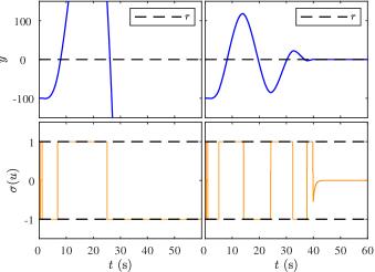
Figure 1: Example 1. Output-feedback adaptive stabilization of a chain of integrators with arbitrary zeros subject to control-magnitude saturation. The plots on the left show an attempt at adaptive stabilization using PCAC without using ICD coefficients, where stabilization is not achieved. The plots on the right show adaptive stabilization using ICD-PCAC.

Example 2.

Comparison of ICD-PCAC and the nested-saturation controller. We reconsider Example 1 but we compare the performance of ICD-PCAC and the nested-saturation controller of [18]. Since ICD-PCAC operates with output feedback, we consider the output-feedback version of [18] presented in [20]. Note that both [18, 20] require the knowledge of the system and are not predictive, whereas ICD-PCAC is an adaptive MPC algorithm. The parameters for the nested-saturation controller of [20] are

$$u_{0}=0,\quad\lambda_{1}=\lambda_{2}=\lambda_{3}=-0.1,$$ (75)

$$\overline{\varepsilon}_{1}=-\underline{\varepsilon}_{1}=0.24,\quad\overline{\varepsilon}_{2}=-\underline{\varepsilon}_{2}=0.25,$$ (76)

$$\overline{\varepsilon}_{3}=-\underline{\varepsilon}_{3}=0.51.$$ (77)

Figure 2 shows $\tilde{y}$ and $u$, where the convergence rate is faster with ICD-PCAC than with the nested-saturation controller.  $\diamond$

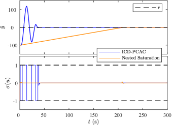
Figure 2: Example 2. Comparison of ICD-PCAC and the nested-saturation controller of [20]. Note that ICD-PCAC is an adaptive MPC algorithm that does not require knowledge of the system, whereas the nested-saturation controller of [20] requires knowledge of the system, and is neither adaptive nor predictive.

Example 3.

Adaptive command following and disturbance rejection. We reconsider Example 1 but where the disturbance, the command, and the sensor noise are nonzero. In particular,

$$d(t)=\sin 10t,\quad r=100,$$ (78)

and the sensor noise $v_{k}$ is a zero-mean, Gaussian white noise with standard deviation $10^{-3}.$ Figure 3 shows adaptive command following and disturbance rejection using ICD-PCAC.  $\diamond$

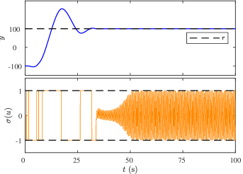
Figure 3: Example 3. Adaptive output-feedback command following and disturbance rejection for a chain of integrators with arbitrary zeros subject to control-magnitude saturation.

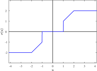
Figure 4: Example 4. Control-magnitude saturation with deadzone input nonlinearity

Example 4.

Adaptive stabilization with abruptly changing command and disturbance in the presence of control-magnitude saturation with deadzone. We reconsider Example 3, where the command and the harmonic disturbance change abruptly at $t=50$ s. In particular,

$$r(t)=\begin{cases}100,&t\leq 50{~{}\rm s},\vspace{1ex}\\ -100,&t>50{~{}\rm s},\end{cases}$$ (79)

and

$$d(t)=\begin{cases}\sin 10t,&t\leq 50{~{}\rm s},\\ 2\sin 5t,&t>50{~{}\rm s}.\end{cases}$$ (80)

Furthermore, the input nonlinearity is control-magnitude saturation with deadzone given by

$$\sigma(u)\triangleq\begin{cases}2,&u>2,\\ u,&1\leq|u|\leq 2,\\ 0,&|u|<1,\\ -2,&u<-2.\end{cases}$$ (81)

Figure 4 shows a plot of $\sigma(u)$ versus $u,$ and Figure 5 shows adaptive command following and disturbance rejection using ICD-PCAC.  $\diamond$

Figure 5: Example 4. Adaptive output-feedback command following and disturbance rejection for a chain of integrators with arbitrary zeros subject to control-magnitude saturation with deadzone, where the command and the disturbance change abruptly at $t=50$ s.

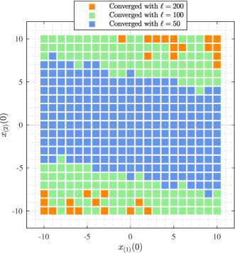
Figure 6: Example 5. Domain of attraction for the nonminimum-phase triple integrator (69) subject to control-magnitude saturation, where the initial conditions are $x_{(1)}(0),x_{(2)}(0)\in[-10,10]$ and $x_{(3)}(0)=0.$ Note that the domain of attraction becomes larger as the horizon $\ell$ of ICD-PCAC increases.

Example 5.

Domain of attraction of ICD-PCAC. We reconsider the chain of integrators in Example 1, and we investigate the domain of attraction using ICD-PCAC. In particular, we consider the grid of initial conditions where $x_{(1)}(0),x_{(2)}(0)\in\{-10,9,\ldots,9,10\}$ and $x_{(3)}(0)=0.$ Each simulation is run for $60$ s, which since $T_{\rm s}=0.1$ s, yields 600 step. The convergence criterion is $\sum_{k=580}^{600}\|x_{k}\|<0.01.$ Figure 6 shows the domain of attraction of ICD-PCAC for $\ell\in\{50,100,200\}$. Numerical simulations with larger values of $\ell$ (not shown) suggest that ICD-PCAC provides semiglobal stabilization.  $\diamond$

IX Conclusions and Future Work

The present paper considered output-feedback control of Hammerstein systems, whose linear dynamics are a priori unknown, but whose input nonlinearity is known. To address this problem, this paper combined predictive cost adaptive control (PCAC) with an iterative receding-horizon optimization technique based on a control-dependent model. In particular, the input nonlinearity was accounted for by using a control-dependent model that replaces the input matrix $B$ with the control-dependent matrix. The control-dependent term is handled through iteration of the receding-horizon optimization, which is performed using quadratic programming (QP). ICD-PCAC was demonstrated numerically by means of several well-known examples. For all of the numerical examples, the iteration was found to converge reliably.

Future research will focus on understanding the reasons for convergence of the iterations involving QP with the control-dependent terms.

References

[1]
W. Kwon and S. Han, Receding Horizon Control: Model Predictive Control
for State Models. Springer, 2006.
[2]
E. F. Camacho and C. Bordons, Model Predictive Control, 2nd ed. Springer, 2007.
[3]
U. Eren, A. Prach, B. B. Koçer, S. V. Raković, E. Kayacan, and
B. Açıkmeşe, “Model predictive control in aerospace systems:
Current state and opportunities,” J. Guid. Contr. Dyn., vol. 40,
no. 7, pp. 1541–1566, 2017.
[4]
M. Lorenzen, M. Cannon, and F. Allgower, “Robust MPC with recursive model
update,” Automatica, vol. 103, pp. 461–471, 2019.
[5]
I. Markovsky, L. Huang, and F. Dorfler, “Data-driven control based on the
behavioral approach: From theory to applications in power systems,”
IEEE Contr. Sys. Mag., vol. 43, pp. 1–35, 2023.
[6]
I. Markovsky and P. Rapisarda, “Data-driven simulation and control,”
Int. J. Contr., vol. 81, no. 12, pp. 1946–1959, 2008.
[7]
J. Berberich, J. Kohler, M. A. Müller, and F. Allgower, “Data-driven model
predictive control with stability and robustness guarantees,” IEEE
Trans. Autom. Contr., vol. 66, no. 4, pp. 1702–1717, 2021.
[8]
D. S. Bernstein and A. N. Michel, “A chronological bibliography on saturating
actuators,” Int. J. Robust Nonlinear Contr., vol. 5, pp. 375–380,
1995.
[9]
S. A. U. Islam and D. S. Bernstein, “Recursive least squares for real-time
implementation,” IEEE Contr. Sys. Mag., vol. 39, no. 3, pp. 82–85,
2019.
[10]
N. Mohseni and D. S. Bernstein, “Recursive least squares with variable-rate
forgetting based on the F-test,” in Proc. Amer. Contr. Conf., 2022,
pp. 3937–3942.
[11]
T. W. Nguyen, S. A. U. Islam, D. S. Bernstein, and I. V. Kolmanovsky,
“Predictive cost adaptive control: A numerical investigation of
persistency, consistency, and exigency,” IEEE Contr. Sys. Mag.,
vol. 41, pp. 64–96, December 2021.
[12]
T. W. Nguyen, I. V. Kolmanovsky, and D. S. Bernstein, “Sampled-data
output-feedback model predictive control of nonlinear plants using online
linear system identification,” in Proc. Amer. Contr. Conf., 2021, pp.
4682–4687.
[13]
S. A. U. Islam, K. Aljanaideh, T. W. Nguyen, I. V. Kolmanovsky, and D. S.
Bernstein, “The free response of an identified model of a linear system with
a completely unknown harmonic disturbance exactly forcasts the
free-plus-forced response of the true system thereby enabling adaptive MPC
for harmonic disturbance rejection,” in Proc. Conf. Dec. Contr.,
2021, pp. 3036–3041.
[14]
D. S. Bernstein and W. M. Haddad, “Nonlinear controllers for positive real
systems with arbitrary input nonlinearities,” IEEE Trans. Autom.
Contr., vol. 39, no. 7, pp. 1513–1517, 1994.
[15]
W. H. Kwon and A. E. Pearson, “On feedback stabilization of time-varying
discrete linear systems,” IEEE Trans. Autom. Contr., vol. AC-23,
no. 3, pp. 479–481, 1978.
[16]
W. Li and E. Todorov, “Iterative linear quadratic regulator design for
nonlinear biological movement systems,” in ICINCO, 2004, pp.
222–229.
[17]
E. Todorov and W. Li, “A generalized iterative LQG method for locally-optimal
feedback control of constrained nonlinear stochastic systems,” in
Proc. Amer. Contr. Conf., 2005, pp. 300–306.
[18]
A. R. Teel, “Global stabilization and restricted tracking for multiple
integrators with bounded controls,” Sys. Contr. Lett., vol. 18,
no. 3, pp. 165–171, 1992.
[19]
T. Lauvdal, R. M. Murray, and T. Fossen, “Stabilization of integrator chains
in the presence of magnitude and rate saturations: a gain scheduling
approach,” in Proc. Conf. Dec. Contr., vol. 4, 1997, pp. 4004–4005.
[20]
M. Kamaldar and D. S. Bernstein, “Dynamic output-feedback control of a chain
of discrete-time integrators with arbitrary zeros and asymmetric input
saturation,” Automatica, vol. 125, p. 109387, 2021.
[21]
J. W. Polderman, “A state space approach to the problem of adaptive pole
assignment,” Mathematics of Control, Signals and Systems, vol. 2,
no. 1, pp. 71–94, 1989.