M-OFDFT: Overcoming the Barrier of Orbital-Free Density Functional Theory for Molecular Systems Using Deep Learning

Abstract

Orbital-free density functional theory (OFDFT) is a quantum chemistry formulation that has a lower cost scaling than the prevailing Kohn-Sham DFT, which is increasingly desired for contemporary molecular research. However, its accuracy is limited by the kinetic energy density functional, which is notoriously hard to approximate for non-periodic molecular systems. In this work, we propose M-OFDFT, an OFDFT approach capable of solving molecular systems using a deep-learning functional model. We build the essential nonlocality into the model, which is made affordable by the concise density representation as expansion coefficients under an atomic basis. With techniques to address unconventional learning challenges therein, M-OFDFT achieves a comparable accuracy with Kohn-Sham DFT on a wide range of molecules untouched by OFDFT before. More attractively, M-OFDFT extrapolates well to molecules much larger than those in training, which unleashes the appealing scaling for studying large molecules including proteins, representing an advancement of the accuracy-efficiency trade-off frontier in quantum chemistry.

1 Introduction

Density functional theory (DFT) is a powerful quantum chemistry method for solving electronic states hence energy and properties of molecular systems. It is among the most popular choices due to its appropriate accuracy-efficiency trade-off, and has fostered many scientific discoveries [1, 2]. The prevailing Kohn-Sham formulation (KSDFT) [3] solves a system by minimizing the electronic energy as a functional of $N$ orbital functions $\{\phi_{i}(\mathbf{r})\}_{i=1}^{N}$, where $N$ is the number of electrons. Although the orbitals allow explicitly calculating the non-interacting part of kinetic energy, optimizing $N$ functions deviates from the original idea of DFT [4, 5, 6, 7] to optimize one function, the (one-body reduced) electron density $\rho(\mathbf{r})$, hence immediately increases the cost scaling by an order of $N$ (Fig. 1(a)). This higher complexity is increasingly undesired for the current research stage where large-scale system simulations for practical applications are in high demand. For this reason, there is a growing interest in methods following the original DFT spirit, now called orbital-free DFT (OFDFT) [8, 9, 10].

The central task in OFDFT is to approximate the non-interacting part of kinetic energy as a density functional (KEDF) $T_{\textnormal{S}}[\rho]$. Classical approximations are developed based on the uniform electron gas theory [11, 12, 13, 14, 15], and have achieved many successes of OFDFT for periodic material systems [16, 17, 10]. But the accuracy is still limited for molecules [18, 19, 20, 21], mainly due to that the electron density in molecules is far from uniform.

For approximating a complicated functional, recent triumphant progress in deep machine learning creates new opportunities. Yet, existing explorations for OFDFT are still in an early stage. These methods use a regular grid to represent density as the model input, which is not efficient enough to represent the uneven density in molecular systems. Even an irregular grid requires unaffordably many points for a nonlocal calculation, while the nonlocality has been found indispensable to approximate KEDF [22, 14, 8, 23]. As a result, these works only studied molecules of up to a dozen atoms, either due to the unaffordable cost of a nonlocal calculation [24, 25, 26, 27, 28] or limited accuracy of a (semi-)local approximation [29, 30, 31, 32]. Moreover, few work showed the accuracy on molecules much larger than those in training, but such an extrapolation study is imperative as it is on molecules larger than other methods could afford to generate abundant data that an OFDFT method could demonstrate the dominating value of its scaling advantage.

In this work, we develop an OFDFT method called M-OFDFT that can handle Molecules using a deep-learning KEDF model. To account for the nonlocal nature of KEDF with affordable cost, we take the expansion coefficients of the density on an atomic basis set as the model input (Fig. 1(b)), which constitute a much more concise representation than a grid-based representation. Each coefficient represents a density component around an atom, and can be treated as a feature associated to that atom. To process such input, we build a deep-learning model based on the Graphormer architecture [33, 34], a variant of Transformer [35] for processing molecular data. The model iteratively processes features on each atom, with the interaction with features on other atoms through the attention mechanism, which covers the nonlocal effect. We note that learning a functional model faces unconventional challenges, for which we propose method to generate multiple density datapoints with gradient labels per molecular structure, and techniques to handle geometric invariance and vast gradient range. After the KEDF model is learned, M-OFDFT solves a given molecular system by optimizing the density coefficients, where the KEDF model is used to construct the energy objective (Fig. 1(c)).

We demonstrate the practical utility and advantage in the following aspects. (1) M-OFDFT achieves chemical accuracy compared to KSDFT on a range of molecular systems in similar scales as those in training. This is hundreds times more accurate than classical OFDFT. The optimized density shows a clear shell structure, which is regarded challenging for an orbital-free approach. (2) M-OFDFT achieves an attractive extrapolation capability that its per-atom error stays constant or even decreases on increasingly larger molecules all the way to 10 times (224 atoms) beyond those in training. The absolute error is still much smaller than classical OFDFT. In contrast, the per-atom error keeps increasing by end-to-end energy prediction counterparts. M-OFDFT also shows a more efficient utilization of a few large-scale data after trained on abundant affordable-scale data. (3) With the accuracy and extrapolation capability, M-OFDFT unleashes the scaling advantage of OFDFT to large-scale molecular systems. We find its empirical time complexity is $O(N^{1.46})$, indeed lower by order-$N$ over $O(N^{2.49})$ of KSDFT. The absolute time is always shorter, achieving a 27.4-fold speedup on the protein B system (2,750 electrons). In all, M-OFDFT pushes the accuracy-efficiency trade-off frontier in quantum chemistry, and provides a powerful tool for solving large-scale molecular science problems.

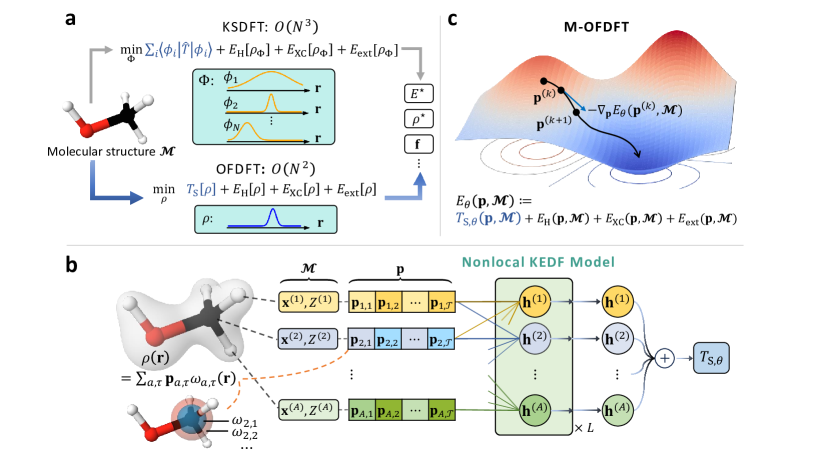
Figure 1: Overview of M-OFDFT. (a) Kohn-Sham DFT solves the properties of a molecular structure $\mathcal{M}$ by optimizing $N$ orbital functions $\{\phi_{i}(\mathbf{r})\}_{i=1}^{N}$, while orbital-free DFT only needs to optimize one density function $\rho(\mathbf{r})$ if the kinetic energy density functional (KEDF) $T_{\textnormal{S}}[\rho]$ is available, which reduces the complexity by an order of $N$. (b) The proposed M-OFDFT uses a deep-learning model to approximate KEDF, which is learned from data. The model incorporates nonlocal interaction of density over the space, which is made affordable by inputting the concise density representation of expansion coefficients $\mathbf{p}$ on an atomic basis $\{\omega_{a,\tau}(\mathbf{r})\}_{a,\tau}$. Each basis function concentrates around an atom, and they altogether span a similar pattern as the density, making the representation concise. (c) M-OFDFT solves a molecular structure $\mathcal{M}$ by optimizing the density coefficients $\mathbf{p}$, for which the learned KEDF model $T_{\textnormal{S},\theta}(\mathbf{p},\mathcal{M})$ constitutes the energy objective.

2 Results

2.1 Overview of M-OFDFT

OFDFT solves the electronic state of a molecular structure $\mathcal{M}$ by minimizing the electronic energy as a functional of the electron density $\rho$, which is typically decomposed in the same way as KSDFT: $E[\rho]=T_{\textnormal{S}}[\rho]+E_{\textnormal{H}}[\rho]+E_{\textnormal{XC}}[\rho]+E_{\textnormal{ext}}[\rho]$, where $T_{\textnormal{S}}[\rho]$ is the kinetic energy density functional (KEDF) covering the non-interacting kinetic energy, $E_{\textnormal{H}}[\rho]$ covers the classical internal potential energy, the exchange-correlation (XC) functional $E_{\textnormal{XC}}[\rho]$ accounts for the rest of kinetic and internal potential energy, and $E_{\textnormal{ext}}[\rho]$ is the external potential energy (Supplementary Sec. A.1). Terms $E_{\textnormal{ext}}[\rho]$ and $E_{\textnormal{H}}[\rho]$ have exact expressions, and $E_{\textnormal{XC}}[\rho]$ already has accurate approximations. As for the non-interacting kinetic energy, in KSDFT it can be calculated from orbital solutions, but as a density functional for conducting OFDFT, the expression $T_{\textnormal{S}}[\rho]$ is unknown and requires an accurate approximation.

The proposed M-OFDFT uses a deep machine learning model to approximate the KEDF (Fig. 1(b)). For an efficient density representation to allow a nonlocal architecture, we adopt an atomic orbital basis set $\{\omega_{\mu}(\mathbf{r})\}_{\mu=1}^{M}$ to expand the density $\rho(\mathbf{r})=\sum_{\mu}\mathbf{p}_{\mu}\omega_{\mu}(\mathbf{r})$, and take the coefficients $\mathbf{p}$ as the model input. Each basis function $\omega_{\mu=(a,\tau)}(\mathbf{r})$ depicts a density pattern $\tau$ around atom $a$, which aligns with the pattern of electron density in a molecule where electrons distribute around atoms. Moreover, they are designed to mimic the nuclear cusp condition [36] for sculpting the sharp density change near a nucleus. They also naturally form a shell structure, i.e., concentrate on different distances from the center atom. These features further fit the details of density in molecules, facilitating the representation with high efficiency. As a result, commonly required basis functions is thousands times fewer than grid points.

Under this representation, the KEDF model follows the form $T_{\textnormal{S},\theta}(\mathbf{p},\mathcal{M})$, where $\theta$ is the learnable parameters, and the molecular structure $\mathcal{M}:=\{\mathbf{X},\mathbf{Z}\}$ is required for specifying the locations and types of basis functions, where $\mathbf{X}:=\{\mathbf{x}^{(a)}\}_{a=1}^{A}$ and $\mathbf{Z}:=\{Z^{(a)}\}_{a=1}^{A}$ are the coordinates and atomic numbers (types) of the atoms (conformation and constitution). As each coefficient $\mathbf{p}_{\mu=(a,\tau)}$ can be associated to one atom $a$, the input $(\mathcal{M},\mathbf{p})$ is a set of pinpointed atoms each with a type and density coefficient features (Fig. 1(b)). To process such input, we build a graph neural network based on the Graphormer architecture [33, 34], which improves graph-theoretical expressiveness over Transformer [35] by incorporating pairwise features (e.g., distance features) into the attention mechanism, the module responsible for nonlocal interactions between density features on two different atoms (Supplementary Sec. B.1). In contrast to commonly used multi-layer perceptrons (MLPs), the Transformer-based model captures “relative relation” instead of “absolute values” of the input feature, which generalizes better for varying-length inputs.This nonlocal formulation has a low cost prefactor by the virtue of the concise density representation, while is indeed crucial for KEDF according to our results in Supplementary Sec. D.4.2.

Perhaps unexpectedly, learning a functional model is more challenging beyond conventional machine learning. Primarily, the model is used as an optimization objective. This requires a higher quality than for end-to-end prediction, as the error would accumulate during optimization hence deviate or even diverge the process. The model needs to capture the energy landscape on the coefficient space, for which only one datapoint per molecular structure is far from sufficient. We hence design methods to produce multiple coefficient data points, each also with a gradient (w.r.t the coefficients) label, for each molecular structure (Methods 4.1). Moreover, the input coefficients are tensors equivariant to the rotation of coordinate system, but the output energy is invariant. To guarantee this geometric invariance in the model, we employ atom-wise local frames. They also stabilize the coefficients for the same type of bonds (Methods 4.2). Finally, the model is aimed at a physical mechanism by which the output energy would increase sharply when the input density deviates from the ground state. To allow the model expressing such large gradients, we introduce a series of enhancement modules that balances the sensitivity over coefficient dimensions, rescales the gradient in each dimension, and offsets the gradient with a reference (Methods 4.3).

After the $T_{\textnormal{S},\theta}(\mathbf{p},\mathcal{M})$ model is learned, M-OFDFT solves the electronic energy and density of a given molecular structure $\mathcal{M}$ through the density optimization procedure (Fig. 1(c)):

$$\min_{\mathbf{p}:\mathbf{p}^{\top}\mathbf{w}=N}E_{\theta}(\mathbf{p},\mathcal{M}):=T_{\textnormal{S},\theta}(\mathbf{p},\mathcal{M})+E_{\textnormal{H}}(\mathbf{p},\mathcal{M})+E_{\textnormal{XC}}(\mathbf{p},\mathcal{M})+E_{\textnormal{ext}}(\mathbf{p},\mathcal{M}),$$ (2)

where $E_{\textnormal{H}}$, $E_{\textnormal{ext}}$ and $E_{\textnormal{XC}}$ can be computed from $(\mathbf{p},\mathcal{M})$ by the conventional way (Supplementary Sec. A.3.2). The constraint on $\mathbf{p}$ fulfills a normalized density, where $\mathbf{w}_{\mu}:=\int\omega_{\mu}(\mathbf{r})\,\mathrm{d}\mathbf{r}$ is the basis normalization vector. The optimization is solved by gradient descent:

$$\mathbf{p}^{(k+1)}:=\mathbf{p}^{(k)}-\varepsilon\left\lparen\mathbf{I}-\frac{\mathbf{w}\mathbf{w}^{\top}}{\mathbf{w}^{\top}\mathbf{w}}\right\rparen\nabla_{\mathbf{p}}E_{\theta}(\mathbf{p}^{(k)},\mathcal{M}),$$ (3)

where $\varepsilon$ is a step size, and the gradient is projected onto the admissible plane in respect to the linear constraint. Notably, due to directly operating on density, the complexity of M-OFDFT in each iteration is $O(N^{2})$ (Supplementary Sec. A.3.2), which is order-$N$ less than that $O(N^{3})$ (with density fitting; Supplementary Sec. A.3.1) of KSDFT.

2.2 M-OFDFT Achieves Chemical Accuracy on Molecular Systems

We first evaluate the performance of M-OFDFT on molecules in similar scales but unseen in training. We generate datasets based on two settings: ethanol structures from the MD17 dataset [37, 38] for studying conformational space generalization, and molecular structures from the QM9 dataset [39, 40] for studying chemical space generalization. Each dataset is split into three parts for the training and validation of the KEDF model, and the test of M-OFDFT. For ease of training, we use the APBE functional [41] as a base KEDF and let the deep-learning model learn the residual (Supplementary Sec. B.4.1).

We evaluate M-OFDFT in terms of the mean absolute error (MAE) from KSDFT results in energy, as well as in the Hellmann-Feynman (HF) force (Supplementary Sec. C.5). The results are 0.18$\,\mathrm{kcal/mol}$ and 1.18$\,\mathrm{kcal/mol/\text{\r{A}}}$ on ethanols, and 0.93$\,\mathrm{kcal/mol}$ and 2.91$\,\mathrm{kcal/mol/\text{\r{A}}}$ on QM9 (Supplementary Sec. D.1.1 shows more results). We see M-OFDFT achieves chemical accuracy (1$\,\mathrm{kcal/mol}$ energy MAE) in both cases.

To show the significance of this result, we compare M-OFDFT with classical OFDFT using well-established KEDFs, including the Thomas-Fermi (TF) KEDF [4, 5] which is exact in the uniform electron gas limit, its corrections TF+$\frac{1}{9}$vW [12] and TF+vW [42] with the von Weizsäcker (vW) KEDF [43], and the base KEDF APBE (Supplementary Sec. C.3). We note that different KEDFs may have different absolute energy biases, so for the energy error we compare the MAE in relative energy. On ethanol structures, the relative energy is taken w.r.t the energy on the equilibrium conformation. On QM9, as each molecule only has one conformation, we evaluate the relative energy between every pair from the 6,095 isomers of $\mathrm{C_{7}H_{10}O_{2}}$ in the QM9 dataset. These isomers can be seen as different conformations of the same set of atoms [44]. As shown in Fig. 2(a), M-OFDFT still achieves chemical accuracy on relative energy, and is two orders more accurate than classical OFDFT.

As a qualitative investigation of M-OFDFT, we visualize the density on a test ethanol structure optimized by these methods in Fig. 2(b) (Supplementary Sec. D.1.2 shows more). Radial density by spherical integral around the oxygen atom is plotted. We find that the M-OFDFT curves coincide with the KSDFT curve precisely. Particularly, the two major peaks around 0 Å and 1.4 Å correspond to the density of core electrons of the oxygen atom and the bonded carbon atom, while the minor peak in between reflects the density of electrons in the covalent bonds with the hydrogen atom and the carbon atom. M-OFDFT successfully recovers this shell structure, which is deemed difficult for OFDFT. In comparison, the classical OFDFT using the APBE KEDF does not align well with the true density around the covalent bonds. These results suggest that M-OFDFT is a working OFDFT for molecular systems.

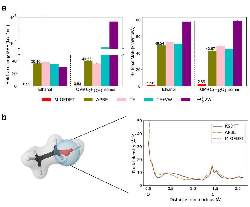
Figure 2: Results of M-OFDFT compared with classical OFDFT on molecular systems. (a) Relative energy and Hellmann-Feynman (HF) force results in mean absolute error (MAE) from KSDFT, with 95% confidence interval bars. (b) Visualization of optimized density. Each curve plots the integrated density on spheres with varying radii centered at the oxygen atom in an ethanol structure.

2.3 M-OFDFT Extrapolates Well to Larger-Scale Molecules

To wield the advantage of the lower cost scaling of M-OFDFT for a more meaningful impact, we evaluate its accuracy on molecular systems with a scale beyond affordable for generating abundant training data. For running on large molecules, we train the deep-learning model targeting the sum of the kinetic and XC energy to get rid of the demanding calculation on grid (Supplementary Sec. B.4.2). This modification does not lead to obvious accuracy lost (Supplementary Sec. D.1.1).

To evaluate the significance of the extrapolation performance, we compare M-OFDFT with a natural variant of deep machine learning method that directly predicts the ground-state energy from the molecular structure $\mathcal{M}$ in an end-to-end manner, which we call M-PES (following “potential energy surface”). We also consider a variant named M-PES-Den that additionally takes the MINAO initialized density into input for investigating the effect of density feature on extrapolation. Both variants use the same nonlocal model architecture and training settings as M-OFDFT for fair comparison (Supplementary Sec. C.4).

QMugs

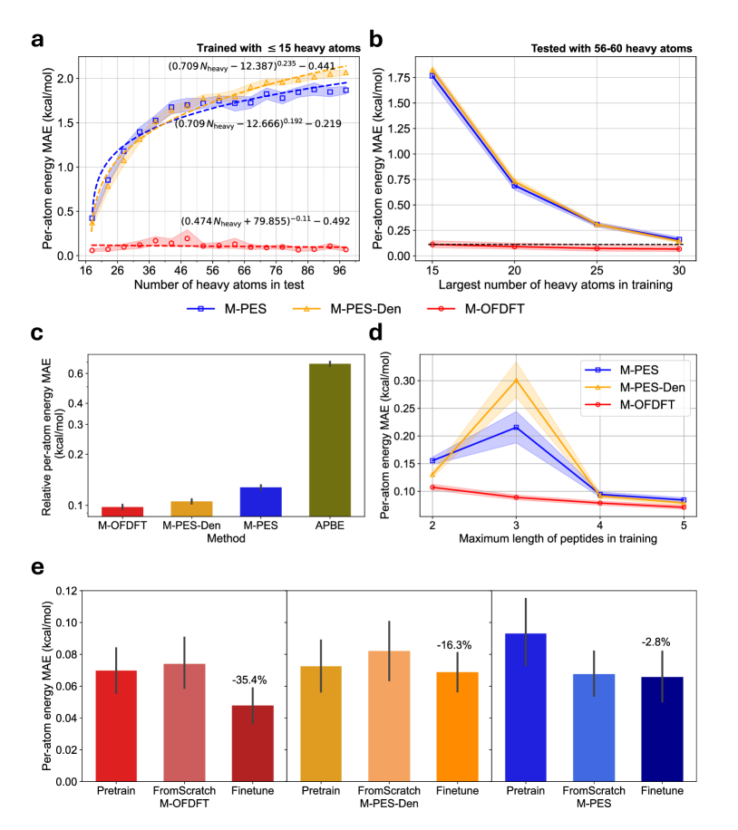
Figure 3: Extrapolation performance of M-OFDFT compared with other deep-learning methods. Considered are M-PES and M-PES-Den that use deep-learning models to predict the ground-state energy end-to-end. The shades and bars show 95% confidence intervals. (a) Mean absolute error (MAE) in per-atom energy on increasingly larger molecules from the QMugs dataset, using models trained on molecules with no more than 15 heavy atoms from QM9 and QMugs datasets. (b) Energy error on 50 QMugs molecules with 56-60 heavy atoms, using models trained on a series of datasets containing increasingly larger QMugs molecules up to 30 heavy atoms. The horizontal dotted black line marks the performance of M-OFDFT trained on the first dataset. (c) Relative energy error on 50 Chignolin structures, using models trained on all peptides (lengths 2-5). Also shown is the result of the classical OFDFT using APBE. (d) Energy error on 1,000 Chignolin structures, using models trained on a series of datasets including increasingly longer peptides. (e) Energy error on 50 Chignolin structures, using models trained on all peptides without (‘Pretrain’) and with ‘Finetune’ on 500 Chignolin structures. Also marked are error reduction ratios by the finetuned models over models trained ‘FromScratch’ on the 500 Chignolin structures only.

We first study the extrapolation on the QMugs dataset [45], containing much larger molecules than those in QM9 which have no more than 9 heavy atoms. We train the models on QM9 together with QMugs molecules with no more than 15 heavy atoms, and test the methods on larger QMugs molecules up to 101 heavy atoms, which are grouped according to the number of heavy atoms into bins of width 5, and are randomly subsampled to ensure the same number (50) of molecular structures in each bin to eliminate statistical effects.

The result is shown in Fig. 3(a). We see that the per-atom MAE of M-OFDFT is always orders smaller than M-PES and M-PES-Den in absolute value, even though M-PES and M-PES-Den achieve a lower validation error (Supplementary Table 6). More attractively, the error of M-OFDFT keeps constant and even decreases (note the negative exponent) when the molecule scale increases, while the errors of M-PES and M-PES-Den keep increasing, even though they use the same nonlocal architecture capable of capturing long-range effects, and M-PES-Den also has a density input. We attribute the qualitatively better extrapolation to appropriately formulating the machine-learning task. The ground-state energy of a molecular structure is the result of an intricate, many-body interaction among electrons and nuclei, leading to a highly challenging function to extrapolate from one region to another. M-OFDFT converts the task into learning the objective function for the target output. The objective only needs to capture the mechanism that the particles interact, which has a reduced level of complexity, while transferring a large portion of complexity to the optimization process, for which optimization tools can handle effectively without an extrapolation issue. Similar phenomena have also been observed recently in machine learning that learning an objective shows better extrapolation than learning an end-to-end map [46, 47].

To further substantiate the significance of the extrapolation capability of M-OFDFT, we investigate the magnitude by which the training molecule scale must be increased for M-PES and M-PES-Den to achieve the same level of performance as M-OFDFT on a given workload of large-scale molecules. We take 50 QMugs molecules with 50-60 heavy atoms as the extrapolation benchmark, and train the models on a series of equal-sized datasets that include increasingly larger molecules up to 30 heavy atoms. As shown in Fig. 3(b), M-PES and M-PES-Den require at least twice as large molecules in the training dataset (30 vs. 15 heavy atoms) to achieve a commensurate accuracy (0.068${\,\mathrm{kcal/mol}}$) as M-OFDFT provides. These extrapolation results suggest that M-OFDFT can be applied to systems much larger than training to exploit the scaling advantage, and is more affordable to develop for solving large-scale molecular systems.

Chignolin

An increasingly important portion of the demand for large-scale quantum chemistry calculation comes from biomolecular systems, particularly proteins, which are not touched by OFDFT previously. We assess the capability of M-OFDFT for protein systems on the Chignolin protein (10 residues, 168 atoms after neutralization). We consider the practical setup that it is unaffordable to generate abundant data for the large target system hence requiring extrapolation. We generate training data on smaller-scale systems of short peptide structures containing 2 to 5 residues, cropped from 1,000 Chignolin structures selected from [48]. To account for non-covalent effects, training data also include systems containing two peptides of lengths 2 and 2, and 2 and 3, where each peptide pair is cropped from the same Chignolin structure. See more details in Supplementary Sec. C.1.4. For this task, we let the model target the total energy for a learning stability consideration (Supplementary Sec. B.4.3).

We first train the model on all available peptides, and compare the relative energy error on Chignolin with other methods in Fig. 3(c). Notably, M-OFDFT achieves a significantly lower per-atom error than the classical OFDFT using the APBE KEDF (0.098${\,\mathrm{kcal/mol}}$ vs. 0.684${\,\mathrm{kcal/mol}}$), providing an effective OFDFT method for biomolecular systems. M-OFDFT also outperforms deep-learning variants M-PES and M-PES-Den, indicating a better extrapolation capability. To investigate extrapolation in more detail, we train the deep-learning models on peptides with increasingly larger scale and plot the error on Chignolin in Fig. 3(d) (similar to the setting of Fig. 3(b)). Remarkably, M-OFDFT consistently outperforms end-to-end energy prediction methods M-PES and M-PES-Den across all lengths of training peptides, and halves the required length for the same level of accuracy. We note the spikes of M-PES and M-PES-Den at peptide length 3 despite extensive hyperparameter tuning, possibly due to that their harder extrapolation difficulty magnifies the gap between in-scale validation and larger-scale performance in this case.

After being trained on data in accessible scale, which is called “pretraining” in the following context, a deep-learning model for a larger-scale workload can be further improved if a few larger-scale data are available for finetuning. In this situation, a method capable of good extrapolation could be roughly aligned with the larger-scale task in advance using accessible data, more efficiently leveraging the limited larger-scale data, and outperforming the model trained from scratch on these limited data only. To investigate the benefit of M-OFDFT in this scenario, we build a finetuning dataset on 500 Chignolin structures. Results in Fig. 3(e) show that M-OFDFT achieves the most gain from pretraining, reducing the energy error by 35.4% over training from scratch, showing the appeal of extracting a more generalizable rule from accessible-scale data. With finetuning, M-OFDFT still gives the best absolute accuracy. These results suggest that M-OFDFT could effectively handle as large a molecular system as a protein, even without abundant training data on the same large scale.

2.4 M-OFDFT Has a Lower Empirical Time Complexity than KSDFT

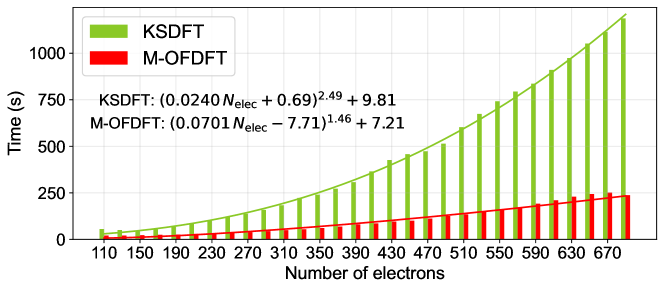
Figure 4: Empirical time cost of M-OFDFT compared with KSDFT on molecules in various scales. Each plotted value is the average of running times on molecules whose number of electrons falls in the corresponding bin of width 20.

After validating the accuracy and extrapolation capability, we now demonstrate the scaling advantage of M-OFDFT empirically. The time cost for running both methods on increasingly large molecules from the QMugs dataset [45] is plotted in Fig. 4. We see the absolute running time of M-OFDFT is always shorter than that of KSDFT, achieving up to 6.7-fold speedup. The empirical complexity of M-OFDFT is $O(N^{1.46})$, which is indeed at least order-$N$ less than the empirical complexity $O(N^{2.49})$ of KSDFT. Supplementary Sec. C.2 details the running setup.

To further wield the advantage, we run M-OFDFT on two molecular systems as large as proteins: (1) the peripheral subunit-binding domain BBL-H142W (PDB ID: 2WXC) [49] containing 2,676 electrons (709 atoms), and (2) the K5I/K39V double mutant of the Albumin binding domain of protein B (PDB ID: 1PRB) [50] containing 2,750 electrons (738 atoms). Such a scale exceeds the typical workload of KSDFT [51]. M-OFDFT costs 0.41 and 0.45 hours on the two systems, while using KSDFT costs 10.5 and 12.3 hours, hence a 25.6-fold and 27.4-fold speedup is achieved. Supplementary Sec. D.3 provides more details.

3 Conclusion and Discussion

This work has developed M-OFDFT, an orbital-free density functional theory that works successfully on molecules. The central task to approximate the kinetic energy density functional (KEDF) is regarded challenging, especially for molecular systems. We have shown that such approximation can be achieved much more accurately by modern deep machine learning models with proper architecture design and training techniques. M-OFDFT achieves working accuracy on molecules and shows desirable extrapolation capability, unleashing the attractive scalability of OFDFT for large molecular systems.

This work introduces a few technical improvements for learning a functional model. Instead of a grid-based representation, we used the density coefficients on an atomic basis as model input, whose much lower dimensionality allows our construction of a nonlocal architecture to enhance accuracy and extrapolation. Some works [52, 53] on learning the XC functional also adopt the coefficient input, but without the molecular structure input, hence cannot properly capture inter-atomic density feature interaction. Regarding the additional challenge for learning an objective, we generated multiple data points each also with a gradient label for each molecular structure. Although the possibility has been noted by previous works [24, 25], none has fully leveraged such abundant data for training (some only incorporated gradient [29, 30, 32, 28]). There are other ways to regularize the optimization behavior of a functional model [54, 55, 56, 53], but our trials in Supplementary Sec. D.4.4 show that they are not as effective. To express intrinsically large gradient, we introduce enhancement modules in addition to a conventional neural network. For stable density optimization using a learned model, prior works [24, 25, 27, 29] used projection onto the training-data manifold in each step, while M-OFDFT only needs the initialization be on the manifold (Methods 4.4).

While statistical guarantees are established for in-distribution generalization [57], reliable extrapolation remains an open challenge and has long bothered the application of machine learning in the science domain [58, 59]. This work has demonstrated the improved extrapolation by choosing an appropriate formulation of quantum chemistry: learning a density functional extrapolates qualitatively better than direct energy prediction. Incorporating exact properties of KEDF into the model also benefits extrapolation. We have geometric invariance built into the model using local frame. Nevertheless, it is not always straightforward to gain benefits from these properties, since some would introduce more training challenges or unintended model capacity restrictions. For example, we tried the von Weizsäcker KEDF as the base KEDF which introduces positivity to the residual model [60, Thm. 1.1], but the resulting gradient labels are too large to learn effectively. The KEDF also has a scaling property, but it cannot be translated into an exact equation under atomic basis (Supplementary Sec. A.5).

For better extrapolation, another possibility from the machine learning perspective is using more data and larger model size with a proper architecture. Recent progress in large language model [61, 62] has shown the emergence of the capacity to solve seemingly all language tasks given large enough data and model. A similar trend in the Graphormer architecture is hinted by a recent study [63] for equilibrium distribution, indicating opportunity to further improve the universality of the functional model.

In summary, M-OFDFT represents an advancement of the frontier of accuracy-efficiency trade-off in quantum chemistry, creating a new powerful tool for exploring large and complex molecules with a higher level of detail and scale.

4 Methods

In response to the more challenges beyond conventional (deep) machine learning, we describe methodological details for KEDF model training (Methods 4.1), additional design for geometric invariance (Methods 4.2) and large gradient capacity (Methods 4.3), and density optimization strategies (Methods 4.4) of M-OFDFT.

4.1 Training the KEDF Model

Although learning the KEDF model $T_{\textnormal{S},\theta}(\mathbf{p},\mathcal{M})$ can be converted to a supervised machine learning task, it is more challenging than the conventional form. The essential difference is rooted in the way that the model is used: instead of as an end-to-end mapping to predict the kinetic energy of $(\mathbf{p},\mathcal{M})$ queries, the model is used as the objective to optimize the density coefficients $\mathbf{p}$ for a given molecular structure $\mathcal{M}$ (Fig. 1(c)). To eliminate instability and achieve accurate optimization result, the model is required to capture how to vary with $\mathbf{p}$ for a fixed $\mathcal{M}$, i.e., the optimization landscape on the coefficient space. Conventional data format $\{\mathcal{M}^{(d)},\mathbf{p}^{(d)},T_{\textnormal{S}}^{(d)}\}_{d}$ does not effectively convey such information, since only one labeled $\mathbf{p}$ data point is seen for each $\mathcal{M}$. Hence the first requirement on training data is multiple coefficient data points per structure, following the format $\{\mathcal{M}^{(d)},\{\mathbf{p}^{(d,k)},T_{\textnormal{S}}^{(d,k)}\}_{k}\}_{d}$. On such data, the model is trained by minimizing:

$$\sum_{d}\sum_{k}\left\lvert T_{\textnormal{S},\theta}(\mathbf{p}^{(d,k)},\mathcal{M}^{(d)})-T_{\textnormal{S}}^{(d,k)}\right\rvert.$$ (4)

After some trials, we found this is still not sufficient. The trained model, although accurately predicts the kinetic energy value, still decreases the electronic energy in density optimization (Eq. (3)) even starting from the ground-state density. This indicates the gradient $\nabla_{\mathbf{p}}T_{\textnormal{S},\theta}(\mathbf{p},\mathcal{M})$ w.r.t the coefficients is still not accurately recovered. We hence also desire a gradient label for each data point, which constitutes data in the format $\{\mathcal{M}^{(d)},\{\mathbf{p}^{(d,k)},T_{\textnormal{S}}^{(d,k)},\nabla_{\mathbf{p}}T_{\textnormal{S}}^{(d,k)}\}_{k}\}_{d}$. As only the projected gradient matters for density optimization following Eq. (3), the gradient data is used for training the model by minimizing:

$$\sum_{d}\sum_{k}\bigg{\lVert}\bigg{(}\mathbf{I}-\frac{\mathbf{w}^{(d)}{\mathbf{w}^{(d)}}^{\top}}{{\mathbf{w}^{(d)}}^{\top}\mathbf{w}^{(d)}}\bigg{)}\Big{(}\nabla_{\mathbf{p}}T_{\textnormal{S},\theta}(\mathbf{p}^{(d,k)},\mathcal{M}^{(d)})-\nabla_{\mathbf{p}}T_{\textnormal{S}}^{(d,k)}\Big{)}\bigg{\rVert}.$$ (5)

The gradient label provides additional information on the local landscape near each coefficient data point. As the model is used in density optimization only through its gradient, the gradient data directly stabilizes and regularizes density optimization, and enforces stationary-point condition for correct convergence. Supplementary Sec. D.4.1 verifies the improvement empirically through an ablation study.

To generate such multiple-coefficient and gradient-labeled data, we note that it is tractable from running the conventional KSDFT on each molecular structure $\mathcal{M}^{(d)}$, which conducts a self-consistent field (SCF) iteration. The rationale is that, the task in each SCF step $k$ is to solve a non-interacting fermion system in an effective one-body potential constructed from previous steps. The ground-state wavefunction solution is a Slater determinant specified by the $N$ orbital solutions in that step, by which the non-interacting kinetic energy $T_{\textnormal{S}}^{(d,k)}$ can be directly calculated. The corresponding density coefficients $\mathbf{p}^{(d,k)}$ can be calculated from these orbitals by density fitting [64]. For the gradient label, since $\mathbf{p}^{(d,k)}$ represents the ground-state density of the non-interacting system, it minimizes the energy of the non-interacting system as a function of density coefficient, $T_{\textnormal{S}}(\mathbf{p},\mathcal{M}^{(d)})+\mathbf{p}^{\top}\mathbf{v}_{\textnormal{eff}}^{(d,k)}$, where $\mathbf{v}_{\textnormal{eff}}^{(d,k)}$ is the effective potential in SCF step $k$ in vector form under the atomic basis. This indicates $\nabla_{\mathbf{p}}T_{\textnormal{S}}(\mathbf{p}^{(d,k)},\mathcal{M}^{(d)})=-\mathbf{v}_{\textnormal{eff}}^{(d,k)}$ up to the normalization projection. Supplementary Sec. A.2 elaborates more on the reasoning, and Supplementary Sec. A.4 provides calculation details, including an efficient implementation to generate the gradient label.

In our implementation of M-OFDFT, the atomic basis for representing density is taken as the even-tempered basis set [65] with tempering ratio $\beta=2.5$. For generating data, restricted-spin KSDFT is conducted at the PBE/6-31G(2df,p) level, which is sufficient for the considered systems which are uncharged, in near-equilibrium conformation, and only involve light atoms (up to fluorine).

4.2 Geometric Invariance

Another challenge beyond conventional machine learning is that the target physical functional exhibits symmetry w.r.t transformations on the input $(\mathbf{p},\mathcal{M}=\{\mathbf{X},\mathbf{Z}\})$ arising from the translation and rotation of the molecule. This is formally referred to as $\mathrm{SE}(3)$-invariance, following “3-dimensional special Euclidean group” that comprises these transformations. This is because the non-interacting kinetic energy of electrons does not change with the translation and rotation of the molecule, but the input atomic coordinates $\mathbf{X}$ do, and the input density coefficients $\mathbf{p}$ also change with the rotation. The change of $\mathbf{p}$ is due to that the electron density rotates with the molecule, but the atomic basis functions do not, since their orientations are aligned with the (global) coordinate system, a.k.a frame. Formally, such input features are geometric vectors and tensors that change equivariantly with the translation and/or rotation of the molecule. Subsequently, the model is expected to have this $\mathrm{SE}(3)$-invariance built-in. This allows the model to learn the essential dependency of the energy on the density irrespective of geometric variability, reducing the problem space, and facilitating data efficiency and effective training. The invariance also enhances generalization and extrapolation performance, as an important physical property is always guaranteed [66, 67].

For the invariance w.r.t atomic coordinates $\mathbf{X}$, the neural network model of Graphormer is naturally $\mathrm{SE}(3)$-invariant, since the model only uses relative distances of atom pairs for later processing, which are inherently invariant w.r.t the translation and rotation of the molecule. To ensure the invariance of the model w.r.t the density coefficients $\mathbf{p}$, we introduce a transformation on $\mathbf{p}$ under local frames to make invariant coefficient features. Each local frame is associated to an atom, and specifies the orientation of atomic basis functions on that atom. It is determined by the relative positions among nearby atoms, hence the basis function orientations rotate with the molecule and the density, making the density coefficients under the local frame invariant. Specifically, the local frame on the atom located at $\mathbf{x}_{a}^{(0)}$ is determined following previous works (e.g., [68, 69]): the x-axis unit vector $\hat{\mathbf{x}}:=\mathrm{Normalize}(\mathbf{x}_{a}^{(1)}-\mathbf{x}_{a}^{(0)})$ is pointed to its nearest heavy atom located at $\mathbf{x}_{a}^{(1)}$, then the z-axis is pointed to $\hat{\mathbf{z}}:=\mathrm{Normalize}\big{(}\hat{\mathbf{x}}\times(\mathbf{x}_{a}^{(2)}-\mathbf{x}_{a}^{(0)})\big{)}$, where $\mathbf{x}_{a}^{(2)}$ is the coordinates of the second-nearest heavy atom not collinear with the nearest one, and finally the y-axis is pointed to $\hat{\mathbf{y}}:=\hat{\mathbf{z}}\times\hat{\mathbf{x}}$ following a right-handed system. See Supplementary Sec. B.2 for more details.

Moreover, the local frame approach offers an additional benefit that the coefficient features are stabilized for local molecular substructures, e.g., bond or functional group, of the same type. Such substructures on one molecule may have different orientations relative to the whole molecule, but the electron density on them are naturally close, up to a rotation. Other invariant implementations, e.g., using an equivariant global frame [70, 71] or processing tensorial input invariantly [72, 73, 74, 75], bind the basis orientations on different atoms together, so the resulting coefficients on the substructures appear vastly different. In contrast, using local frames, basis orientations on different atoms are decoupled, and since they are determined only by nearby atoms, the basis functions rotate from one substructure to another accordingly. Hence, the resulting density coefficients are aligned together, whose difference only indicates the minor density fluctuation on the same type of substructure but not the different orientations of the copies. This makes the model much easier to identify that such local density components follow the same pattern and contribute similarly to the energy. Supplementary Sec. B.2 provides an illustrative explanation. We numerically demonstrate the benefit in Supplementary Figs. 9-10 that using local frame instead of equivariant global frame significantly reduces the variance of both density coefficients and gradients on atoms of each type. Especially, on most basis functions of hydrogen, the coefficient and gradient scales are reduced by over 60%. This significantly stabilizes the training process and immediately reduces training error, resulting in a considerable improvement of overall performance as empirically verified in Supplementary Sec. D.4.3.

4.3 Enhancement Modules for Vast Gradient Range

After reducing the geometric variability of data using local frame, the raw gradient values still show a vast range, which conventional neural networks are not designed for (e.g., [76]) and indeed causes training difficulties in our trials. This is an intrinsic challenge for learning a physical functional since we require non-ground-state density in the data, which would increase the energy steeply. The large gradient range cannot be trivially reduced by conventional data normalization techniques, since its scale is associated with the scale of energy and coefficient, hence downscaling the gradient would either proportionally downscale the energy values which requires a higher prediction resolution, or inverse-proportionally upscale the coefficients which is also numerically unfriendly to process. To handle this challenge, we introduce a series of enhancement modules to allow expressing a vast gradient range, including dimension-wise rescaling, a reparameterization of the density coefficients, and an atomic reference module to offset the large mean of gradient.

Dimension-wise Rescaling

We first upgrade data normalization more flexibly to trade-off coefficient-gradient scales dimension-wise. Considering the number of coefficient dimensions vary from different molecules, we propose to center and rescale the coefficients using biases $\bar{\mathbf{p}}_{Z,\tau}$ and factors $\lambda_{Z,\tau}$ each specific to one coefficient/gradient dimension $\tau$ associated with one atom type (i.e., chemical element) $Z$ but not one atom. The bias $\bar{\mathbf{p}}_{Z,\tau}:=\mathrm{mean}\{\mathbf{p}_{a,\tau}^{(d,k)}\}_{a:Z^{(a)}=Z,\;k,\,d}$ for $(Z,\tau)$ is the average over coefficient values in dimension $\tau$ on all atoms of type $Z$ in all molecular structures in the training dataset. After centering the coefficients using the bias (which does not affect gradients), the scaling factor $\lambda_{Z,\tau}$ is determined by upscaling the centered coefficient and simultaneously inverse-proportionally downscaling the gradient, until the gradient achieves a chosen target scale $s_{\textnormal{grad}}$ or the coefficient exceeds a chosen maximal scale $s_{\textnormal{coeff}}$. In equation:

$$\lambda_{Z,\tau}=\begin{dcases}\min\bigg{\{}\frac{\mathrm{max\_grad}_{Z,\tau}}{s_{\textnormal{grad}}},\,\frac{s_{\textnormal{coeff}}}{\mathrm{std\_coeff}_{Z,\tau}}\bigg{\}},&\text{if }\mathrm{max\_grad}_{Z,\tau}>s_{\textnormal{grad}},\\ 1,&\text{otherwise},\end{dcases}$$ (6)

where the scales of gradient and coefficient for $(Z,\tau)$ are measured by the maximum of gradient $\mathrm{max\_grad}_{Z,\tau}:=\max\{\nabla_{\mathbf{p}_{a,\tau}}T_{\textnormal{S}}^{(d,k)}\}_{a:Z^{(a)}=Z,\;k,\,d}$ and standard derivation of coefficient $\mathrm{std\_coeff}_{Z,\tau}:=\mathrm{std}\{\mathbf{p}_{a,\tau}^{(d,k)}\}_{a:Z^{(a)}=Z,\;k,\,d}$ on the dataset. Using the rescaling factors, each centered coefficient is rescaled by $\mathbf{p}^{\prime}_{a,\tau}:=\lambda_{Z^{(a)},\tau}\,\mathbf{p}_{a,\tau}$, and gradient by $\nabla_{\mathbf{p}_{a,\tau}}T_{\textnormal{S}}^{\prime}:=\nabla_{\mathbf{p}_{a,\tau}}T_{\textnormal{S}}\,/\,\lambda_{Z^{(a)},\tau}$ ($\lambda_{Z,\tau}>1$ in most cases).

Natural Reparameterization

On quite a few dimensions, both the coefficient and gradient scales are large, making dimension-wise rescaling ineffective. We hence introduce natural reparameterization applied before rescaling to balance the rescaling difficulties across dimensions hence reduce the worst-case difficulty. The unbalanced scales come from the different sensitivities of the density function on different coefficient dimensions: the change of density function from a coefficients change $\Delta\mathbf{p}$ is measured by the L2-metric in the function space, $\int\left\lvert\Delta\rho(\mathbf{r})\right\rvert^{2}\,\mathrm{d}\mathbf{r}$, which turns out to be $\Delta\mathbf{p}^{\top}\mathbf{W}\Delta\mathbf{p}$, in which different dimensions indeed contribute with different weights since the overlap matrix $\mathbf{W}_{\mu\nu}:=\int\omega_{\mu}(\mathbf{r})\omega_{\nu}(\mathbf{r})\,\mathrm{d}\mathbf{r}$ therein is generally anisotropic. The reparameterized coefficients $\tilde{\mathbf{p}}$ are expected to contribute equally across the dimensions: $\int\left\lvert\Delta\rho(\mathbf{r})\right\rvert^{2}\,\mathrm{d}\mathbf{r}=\Delta\tilde{\mathbf{p}}^{\top}\Delta\tilde{\mathbf{p}}$. We hence take:

$$\tilde{\mathbf{p}}:=\mathbf{M}^{\top}\mathbf{p},$$ (7)

where $\mathbf{M}$ is a square matrix satisfying $\mathbf{M}\mathbf{M}^{\top}=\mathbf{W}$. See Supplementary Sec. B.3.2 for more details. This reparameterization also leads to natural gradient descent [77] in density optimization, which is known to converge faster than vanilla gradient descent.

Atomic Reference Module

Recall that in dimension-wise rescaling, the large bias of coefficients can be offset by the mean on a dataset, but this does not reduce the bias scale of gradient labels. To further improve the coefficient-gradient scale trade-off, we introduce an atomic reference module:

$$T_{\mathrm{AtomRef}}(\mathbf{p},\mathcal{M}):=\bar{\mathbf{g}}_{\mathcal{M}}^{\top}\mathbf{p}+\bar{T}_{\mathcal{M}},$$ (8)

which is linear in the coefficients $\mathbf{p}$ and whose output is added to the neural network output as the kinetic energy value. By this design, the gradient of the atomic reference model $\nabla_{\mathbf{p}}T_{\mathrm{AtomRef}}(\mathbf{p},\mathcal{M})=\bar{\mathbf{g}}_{\mathcal{M}}$ is a constant, which offsets the target gradient for the neural network to capture, effectively reducing the scale of gradient labels and facilitating neural network training. The weights $\bar{\mathbf{g}}_{\mathcal{M}}:=\mathrm{concat}\{\bar{\mathbf{g}}_{Z^{(a)},\tau}\}_{\tau,\,a\in\mathcal{M}}$ and bias $\bar{T}_{\mathcal{M}}:=\sum_{a\in\mathcal{M}}\bar{T}_{Z^{(a)}}+\bar{T}_{\mathrm{global}}$ of the linear model are constructed by tiling and summing the per-type statistics, which are derived over all atoms of each type in a dataset. The per-type gradient statistics is defined by $\bar{\mathbf{g}}_{Z,\tau}:=\mathrm{mean}\{\nabla_{\mathbf{p}_{a,\tau}}T_{\textnormal{S}}^{(d,k)}\}_{a:Z^{(a)}=Z,\;k,\,d}$, which represents the average response to $T_{\textnormal{S}}$ from the change of coefficients on an atom of type $Z$. Per-type bias statistics $\{\bar{T}_{Z}\}_{Z}$ and $\bar{T}_{\mathrm{global}}$ are fit by least squares. See Supplementary Sec. B.3.3 for more details.

The final KEDF model is constructed from these enhancement modules and the neural network model in the following way (Supplementary Fig. 6(a)): the density coefficients are first transformed under local frame and processed by natural reparameterization; the processed coefficients, through one branch, are fed to the atomic reference module to calculate the reference part of output energy, and through another branch, are processed by dimension-wise rescaling and then input to the neural network model which produces the rest part of output energy. Comparative results in Supplementary Sec. B.3 and D.4.3 highlight the empirical benefits of each module.

4.4 Density Optimization

In the deployment stage, M-OFDFT solves the ground state of a given molecular structure $\mathcal{M}$ by minimizing the electronic energy as a function of density coefficients $\mathbf{p}$, where the learned KEDF model $T_{\textnormal{S},\theta}(\mathbf{p},\mathcal{M})$ is used to construct the energy function (Fig. 1(a)). As described in Results 2.1, we use gradient descent to optimize $\mathbf{p}$ (Eq. (3)), since it is unnatural to formulate the optimization problem into a self-consistent iteration. Gradient descent has also been used in KSDFT, which bears the merit of being more stable [78].

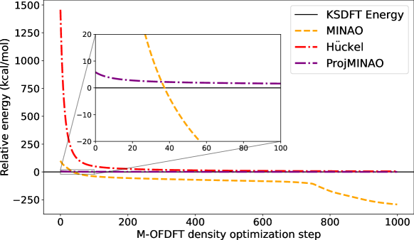
Figure 5: Typical density optimization curves of M-OFDFT for a QM9 molecule with different initialization methods. MINAO, the common KSDFT initialization, leads the optimization to a large gap from the target energy, since it is not from the eigensolution to an effective Hamiltonian matrix, hence lies off the training-data manifold (out of distribution). Hückel initialization solves an eigenvalue problem, which indeed converges the curve with a much smaller energy error of 5.34 $\mathrm{kcal/mol}$. ProjMINAO initialization uses a deep-learning model to project the MINAO density onto the training-data manifold, which also converges the curve and achieves the best result of 0.60 $\mathrm{kcal/mol}$ energy error. The inset figure highlights the role of density optimization even though the ProjMINAO density is close to the ground-state density.

A subtlety in density optimization using a learned functional model is that the model may be confronted with densities far from the training-data manifold (or “out of distribution” in machine-learning term), which may lead to unstable optimization. Such an issue has been observed in previous machine-learning OFDFT [24, 25, 27], which mitigates the problem by projecting the density onto the training-data manifold in each optimization step. A similar phenomenon is also observed in M-OFDFT. As shown in Fig. 5, when starting from the MINAO initialization [79] which is common for KSDFT, the density optimization process leads to an obvious gap from the target KSDFT energy. We note that the initial density by MINAO already lies off the manifold inherently: each density entry in the training data comes from the eigensolution to an effective one-electron Hamiltonian matrix, which exactly solves an effective non-interacting fermion system (Supplementary Sec. A.2),while the MINAO density comes from the superposition of orbitals of each atom in isolation, which is a different mechanism.

We hence propose using two other initialization methods to resolve the mismatch. The first approach is to use an established initialization that solves an eigenvalue problem, for which we choose the Hückel initialization [80, 81]. As shown in Fig. 5, although the Hückel density shows a much larger energy error than MINAO density at initialization, it ultimately indeed leads the optimization process to converge closely to the target energy.

The second choice is to project the MINAO density onto the training-data manifold, which we call ProjMINAO. In contrast to previous methods, M-OFDFT conducts optimization on the coefficient space which varies with molecular structure, so the training-data manifold of coefficient is unknown for an unseen molecular structure. We hence use another deep-learning model $\Delta\mathbf{p}_{\theta}(\mathbf{p},\mathcal{M})$ to predict the required correction to project the input coefficient $\mathbf{p}$ towards the ground-state coefficient $\mathbf{p}^{\star}$ of the input molecular structure $\mathcal{M}$, which is always on the manifold. See Supplementary Sec. B.5.2 for details. From Fig. 5, we see ProjMINAO initialization indeed converges the optimization curve close to the target energy, even better than Hückel initialization. Note that even though ProjMINAO already closely approximates the ground state density, density optimization still continues to improve the accuracy. This suggests a potential advantage over end-to-end ground-state density prediction followed by energy prediction from ground-state density, which may also encounter extrapolation challenges similar to M-PES and M-PES-Den. Remarkably, Fig. 5 indicates that M-OFDFT only requires an on-manifold initialization but does not need projection in each optimization step, suggesting better robustness than previous methods. M-OFDFT in Results 2 is conducted using ProjMINAO, although using Hückel still achieves a reasonable accuracy; see Supplementary Sec. D.1.1. Supplementary Sec. B.5.1 provides curves in density error and comparison with classical KEDFs.

Author information

Author contributions

C.Liu led the research under the support from B.Shao and N.Zheng. C.Liu, S.Zheng and B.Shao conceived the project. H.Zhang, S.Zheng and J.You designed and implemented the deep-learning model. S.Liu, C.Liu, H.Zhang and J.You derived and implemented methods for data generation, the enhancement modules, training pipeline, and density optimization. H.Zhang and S.Liu conducted the experiments. Z.Lu and T.Wang contributed to the experiment design and evaluation protocol. C.Liu, H.Zhang, S.Liu and S.Zheng wrote the paper with inputs from all the authors.

Corresponding authors

Correspondence to Chang Liu, Shuxin Zheng, and Bin Shao.

Appendix

Table 1: Notations

Basic concepts
$\mathbf{r}\in\mathbb{R}^{3}$	Electron coordinate
$N$	Number of electrons in a molecular system
$\psi(\mathbf{r}^{(1)},\cdots,\mathbf{r}^{(N)})$	$N$-electron wavefunction
$\left\langle f\middle|g\right\rangle:=\int f(\mathbf{r})g(\mathbf{r})\,\mathrm{d}\mathbf{r}$	The standard inner product in function space
$\langle f|\hat{O}|g\rangle:=\int f(\mathbf{r})(\hat{O}g)(\mathbf{r})\,\mathrm{d}\mathbf{r}$	Function-space inner product with operator
$(f|g):=\int\frac{f(\mathbf{r})g(\mathbf{r}^{\prime})}{\left\lVert\mathbf{r}-\mathbf{r}^{\prime}\right\rVert}\,\mathrm{d}\mathbf{r}\mathrm{d}\mathbf{r}^{\prime}$	Coulomb integral
Molecular system
$\mathbf{x}\in\mathbb{R}^{3}$	Atom coordinates
$a,b\in\{1,\,2,\,\cdots,A\}$	Indices for atoms in a molecule
$\mathbf{X}:=\{\mathbf{x}^{(a)}\}_{a=1}^{A}$	Molecular conformation/geometry
$\mathbf{Z}:=\{Z^{(a)}\}_{a=1}^{A}$	Molecular composition
$\mathcal{M}:=\{\mathbf{X},\mathbf{Z}\}$	Molecular structure
$\{\mathcal{M}^{(d)}\}_{d=1}^{D}$	Molecular structures in a dataset
Density functional theory
$\Phi:=\{\phi_{i}(\mathbf{r})\}_{i=1}^{N}$	Orbitals
$i,j\in\{1,\,2,\,\cdots,N\}$	Indices for orbitals or electrons
$\psi_{[\Phi]}(\mathbf{r}^{(1)},\cdots,\mathbf{r}^{(N)}):=\det[\phi_{i}(\mathbf{r}^{(j)})]_{ij}$	Slater determinant from orbitals $\Phi=\{\phi_{i}(\mathbf{r})\}_{i=1}^{N}$
$\{\eta_{\alpha}(\mathbf{r})\}_{\alpha=1}^{B}$	Orbital basis
Subscripts $\alpha,\,\beta,\,\gamma,\,\delta\in\{1,\,2,\,\cdots,B\}$	Indices for orbital basis
$\mathbf{C}_{\alpha i}$	Orbital coefficients
$\mathbf{\Gamma}_{\alpha\beta}:=\sum_{i=1}^{N}\mathbf{C}_{\alpha i}\mathbf{C}_{\beta i}$	Density matrix
$\mathbf{S}_{\alpha\beta}:=\left\langle\eta_{\alpha}\middle|\eta_{\beta}\right\rangle$	Overlap matrix of orbital basis
$\mathbf{D}_{\alpha\beta,\gamma\delta}:=\left\langle\eta_{\alpha}\eta_{\beta}\middle|\eta_{\gamma}\eta_{\delta}\right\rangle$	Overlap matrix of paired orbital basis
$\tilde{\mathbf{D}}_{\alpha\beta,\gamma\delta}:=(\eta_{\alpha}\eta_{\beta}|\eta_{\gamma}\eta_{\delta})$	4-center-2-electron Coulomb integral of orbital basis
$\rho(\mathbf{r})$	(One-electron reduced) density (function)
$\{\omega_{\mu}(\mathbf{r})\}_{\mu=1}^{M}$	Density basis
Subscripts $\mu,\nu\in\{1,\,2,\,\cdots,M\}$	Indices for density basis
Subscript $\mu=(a,\tau)$	Atom assignment decomposition of basis index
$\mathbf{p}_{\mu}$	Density coefficient
$\mathbf{w}_{\mu}:=\int\omega_{\mu}(\mathbf{r})\,\mathrm{d}\mathbf{r}$	Density basis normalization vector
$\mathbf{W}_{\mu\nu}:=\left\langle\omega_{\mu}\middle|\omega_{\nu}\right\rangle$	Overlap matrix of density basis
$\tilde{\mathbf{W}}_{\mu\nu}:=(\omega_{\mu}|\omega_{\nu})$	2-center-2-electron Coulomb integral of density basis
$\mathbf{L}_{\mu,\alpha\beta}:=\left\langle\omega_{\mu}\middle|\eta_{\alpha}\eta_{\beta}\right\rangle$	Overlap matrix between density basis and orbital basis
$\mathbf{F}$	Fock matrix in KSDFT
$k$	Step index for SCF iteration or density optimization process
	($\star$ for the converged step)
$(\mathbf{V}_{\textnormal{eff}})_{\alpha\beta}:=\langle\eta_{\alpha}|V_{\textnormal{eff}}|\eta_{\beta}\rangle$	Effective potential matrix under orbital basis
$(\mathbf{v}_{\textnormal{eff}})_{\mu}:=\langle\omega_{\mu}|V_{\textnormal{eff}}\rangle$	Effective potential vector under density basis
$\mu\in\mathbb{R}$	Chemical potential
$\bm{\upvarepsilon}:=\operatorname{Diag}[\varepsilon_{1},\cdots,\varepsilon_{N}]$	The diagonal $N\times N$ matrix of orbital energies
$U[\rho]$	Universal functional
$E_{\textnormal{XC}}[\rho]$	Exchange-correlation (XC) functional
$T_{\textnormal{S}}[\rho]$	Kinetic energy density functional (KEDF)
$T_{\textnormal{S}}(\mathbf{p},\mathcal{M})$	KEDF under atomic basis of density
$T_{\textnormal{S},\theta}(\mathbf{p},\mathcal{M})$	KEDF model/approximation
$T_{\textnormal{APBE}}$	The APBE kinetic functional as the base functional $T_{\textnormal{S,base}}$
$T_{\textnormal{S,res}}$	Residual KEDF on top of the base functional $T_{\textnormal{S,base}}$
$E_{\textnormal{TXC}}$	Kinetic and XC functional
$\mathbf{f}$	Hellmann-Feynman force

Appendix A Mechanism of Density Functional Theory

In this section, we introduce details in relevant theory on DFT, including the formulation of OFDFT under atomic basis, and the mechanism and details to use KSDFT to generate value and gradient data for learning KEDF. Atomic units are used through out the paper.

A.1 Basic Formulation of Density Functional Theory

For brevity, the following formulation is for spinless fermions therefore only consider spacial states. For the restricted Kohn-Sham calculation we adopt for data generation, a pair of electrons of opposite spins share a common spacial orbital, which amounts to duplicate the orbitals in the following formulation.

The mechanism of DFT may be more intuitively introduced under Levy’s constrained search formulation [82]. The $N$-electron Schrödinger equation for ground state is equivalent to the following optimization problem on $N$-electron wavefunctions $\psi(\mathbf{r}^{(1)},\cdots,\mathbf{r}^{(N)})$ under the variational principle:

$$E^{\star}=\min_{\psi:\,\text{antisym},\left\langle\psi\middle|\psi\right\rangle=1}\langle\psi|\hat{T}+\hat{V}_{\textnormal{ee}}+\hat{V}_{\textnormal{ext}}|\psi\rangle,$$ (9)

where $\hat{T}:=-\frac{1}{2}\sum_{i=1}^{N}{\nabla^{(i)}}^{2}$ is the kinetic operator, $\hat{V}_{\textnormal{ee}}:=\sum_{1\leqslant i<j\leqslant N}\frac{1}{\lVert\mathbf{r}^{(i)}-\mathbf{r}^{(j)}\rVert}$ is the electron-electron Coulomb interaction (internal potential), and $\hat{V}_{\textnormal{ext}}:=\sum_{i=1}^{N}V_{\textnormal{ext}}(\mathbf{r}^{(i)})$ comes from a one-body external potential $V_{\textnormal{ext}}(\mathbf{r})$ that commonly arises from the electrostatic field of the nuclei specified by the given molecular structure $\mathcal{M}=\{\mathbf{X},\mathbf{Z}\}$ where $\mathbf{X}:=(\mathbf{x}^{(1)},\cdots,\mathbf{x}^{(A)})$ and $\mathbf{Z}:=(Z^{(1)},\cdots,Z^{(A)})$:

$$V_{\textnormal{ext}}(\mathbf{r})=-\sum_{a=1}^{A}\frac{Z^{(a)}}{\left\lVert\mathbf{r}-\mathbf{x}^{(a)}\right\rVert}.$$ (10)

Although the optimization problem is exactly defined, directly optimizing the $N$-electron wavefunction is very challenging computationally. Specifying the wavefunction $\psi$ and evaluating the energy already require an exponential cost in principle, as $\psi$ is a function on $\mathbb{R}^{3N}$ whose dimension increases with $N$. To make an easier optimization problem, it is then desired to optimize a functional of the one-electron reduced density,

$$\rho_{[\psi]}(\mathbf{r}):=N\int\lvert\psi(\mathbf{r},\mathbf{r}^{(2)},\cdots,\mathbf{r}^{(N)})\rvert^{2}\,\mathrm{d}\mathbf{r}^{(2)}\cdots\mathrm{d}\mathbf{r}^{(N)},$$ (11)

which has an intuitive physical interpretation of charge density even under a classical view, and more importantly, the cost to specify a density is constant (w.r.t $N$) in principle, as the density is a function on $\mathbb{R}^{3}$ whose dimension is constant. This is the starting point of density functional theory (DFT) [4, 5, 6], and is first formally verified by Hohenberg and Kohn [7].

In terms of the density, the external potential energy, i.e., the last term in Eq. (9), is already an explicit density functional, since the external potential is one-body:

$$\langle\psi|\hat{V}_{\textnormal{ext}}|\psi\rangle=\int\rho_{[\psi]}(\mathbf{r})V_{\textnormal{ext}}(\mathbf{r})\,\mathrm{d}\mathbf{r}=E_{\textnormal{ext}}[\rho_{[\psi]}],\quad\text{where }E_{\textnormal{ext}}[\rho]:=\int\rho(\mathbf{r})V_{\textnormal{ext}}(\mathbf{r})\,\mathrm{d}\mathbf{r}.$$ (12)

For the other energy terms, using the density as an intermediate, the optimization problem in Eq. (9) can be equivalently carried out in two levels:

$$E^{\star} =\min_{\rho:\geqslant 0,\int\rho(\mathbf{r})\,\mathrm{d}\mathbf{r}=N}\Big{\lparen}\min_{\psi:\,\text{antisym},\rho_{[\psi]}=\rho}\langle\psi|\hat{T}+\hat{V}_{\textnormal{ee}}|\psi\rangle\Big{\rparen}+E_{\textnormal{ext}}[\rho]$$ (13)

$$=\min_{\rho:\geqslant 0,\int\rho(\mathbf{r})\,\mathrm{d}\mathbf{r}=N}\bigg{\{}E[\rho]:=U[\rho]+E_{\textnormal{ext}}[\rho]\bigg{\}}.$$ (14)

Here, the result of the first-level optimization problem carrying out a constrained search in Eq. (13) defines a density functional,

$$U[\rho]:=\min_{\psi:\,\text{antisym},\rho_{[\psi]}=\rho}\langle\psi|\hat{T}+\hat{V}_{\textnormal{ee}}|\psi\rangle,$$ (15)

called the universal functional, as it is independent of system specification (i.e., $\mathcal{M}$ or $V_{\textnormal{ext}}$). It is composed of the kinetic and internal potential energy of the electrons. The optimization objective is then formally converted to a density functional $E[\rho]$ as shown in Eq. (14).

To carry out practical computation, variants of the kinetic and internal potential energy that allow explicit calculation or have known properties are introduced, to cover the major part of the corresponding energies in $U[\rho]$. The internal potential energy is covered by its classical version, i.e. assuming no correlation, called the Hartree energy:

$$E_{\textnormal{H}}[\rho]:=\frac{1}{2}\int\frac{\rho(\mathbf{r})\rho(\mathbf{r}^{\prime})}{\left\lVert\mathbf{r}-\mathbf{r}^{\prime}\right\rVert}\,\mathrm{d}\mathbf{r}\mathrm{d}\mathbf{r}^{\prime}.$$ (16)

The kinetic energy is covered by the kinetic energy density functional (KEDF), which is defined in a similar way as the universal functional:

$$T_{\textnormal{S}}[\rho]:=\min_{\psi:\,\text{antisym},\rho_{[\psi]}=\rho}\langle\psi|\hat{T}|\psi\rangle.$$ (17)

The remainder in the universal functional is called the exchange-correlation (XC) functional:

$$E_{\textnormal{XC}}[\rho]:=U[\rho]-T_{\textnormal{S}}[\rho]-E_{\textnormal{H}}[\rho],$$ (18)

which is by definition also a density functional. Under this decomposition, the density optimization problem in Eq. (14) becomes:

$$E^{\star}=\min_{\rho:\geqslant 0,\int\rho(\mathbf{r})\,\mathrm{d}\mathbf{r}=N}\bigg{\{}E[\rho]=T_{\textnormal{S}}[\rho]+\underbrace{E_{\textnormal{H}}[\rho]+E_{\textnormal{XC}}[\rho]+E_{\textnormal{ext}}[\rho]}_{=:E_{\textnormal{eff}}[\rho]}\bigg{\}}.$$ (19)

Here $E_{\textnormal{eff}}[\rho]$ is defined for future convenience and denoted after the effective-potential interpretation of its variation detailed later. Using carefully designed explicit expressions or machine-learning models to approximate the $T_{\textnormal{S}}[\rho]$ and $E_{\textnormal{XC}}[\rho]$ functionals, practical computation can be conducted. This is the formulation of orbital-free density functional theory (OFDFT). Indeed, the object to be optimized is the electron density, which is one function on the constant-dimensional space of $\mathbb{R}^{3}$, hence greatly reduces computation complexity over the original variational problem Eq. (9). Under properly designed $T_{\textnormal{S}}[\rho]$ and $E_{\textnormal{XC}}[\rho]$ approximations, the complexity is favorably $O(N^{2})$ under atomic basis.

Considering the KEDF $T_{\textnormal{S}}[\rho]$ is more challenging to approximate than the XC functional $E_{\textnormal{XC}}[\rho]$, Kohn and Sham [3] leverage an equivalent formulation of KEDF to allow its accurate calculation, at the cost of increasing the complexity. The alternative formulation optimizes determinantal wavefunctions. A determinantal wavefunction for $N$ electrons is specified by $N$ one-electron wavefunctions $\Phi:=\{\phi_{i}(\mathbf{r})\}_{i=1}^{N}$, a.k.a orbitals, following the form:

$$\psi_{[\Phi]}(\mathbf{r}^{(1)},\cdots,\mathbf{r}^{(N)}):=\frac{1}{\sqrt{N!}}\det[\phi_{i}(\mathbf{r}^{(j)})]_{ij},\quad\text{given orbitals }\Phi:=\{\phi_{i}(\mathbf{r})\}_{i=1}^{N}.$$ (20)

The equivalent optimization problem in parallel with Eq. (17) is:

$$T_{\textnormal{S}}[\rho]=\min_{\{\phi_{i}\}_{i=1}^{N}:\rho_{[\Phi]}=\rho}\langle\psi_{[\Phi]}|\hat{T}|\psi_{[\Phi]}\rangle=\min_{\vbox{\Let@\restore@math@cr\default@tag\halign{\hfil$\m@th\scriptstyle#$&$\m@th\scriptstyle{}#$\hfil\cr\{\phi_{i}\}_{i=1}^{N}:&\text{orthonormal},\\ &\rho_{[\Phi]}=\rho\crcr}}}\sum_{i=1}^{N}\langle\phi_{i}|\hat{T}|\phi_{i}\rangle,$$ (23)

where $$\rho_{[\Phi]}(\mathbf{r}):=\sum_{i=1}^{N}\left\lvert\phi_{i}(\mathbf{r})\right\rvert^{2},\quad\text{given orthonormal orbitals }\Phi:=\{\phi_{i}(\mathbf{r})\}_{i=1}^{N}.$$ (24)

In Eq. (23), the second equality holds since the density normalizes to $N$, and a set of (non-collinear) functions can always be orthogonalized, e.g., using the Gram-Schmidt process ([83, Sec. 3.1.4]; [84, Sec. 14.3]). This equivalence can be understood from the interpretation of $T_{\textnormal{S}}[\rho]$ as the non-interacting portion of kinetic energy. Indeed, for a non-interacting system, there are only kinetic energy and external potential energy (i.e., taking $\hat{V}_{\textnormal{ee}}=0$), so the two-level optimization in parallel with Eq. (13) becomes:

$$E^{\star} =\min_{\psi:\,\text{antisym},\left\langle\psi\middle|\psi\right\rangle=1}\langle\psi|\hat{T}+\hat{V}_{\textnormal{ext}}|\psi\rangle$$ (25)

$$=\min_{\rho:\geqslant 0,\int\rho(\mathbf{r})\,\mathrm{d}\mathbf{r}=N}\Big{\lparen}\min_{\psi:\,\text{antisym},\rho_{[\psi]}=\rho}\langle\psi|\hat{T}|\psi\rangle\Big{\rparen}+E_{\textnormal{ext}}[\rho]$$ (26)

$$=\min_{\rho:\geqslant 0,\int\rho(\mathbf{r})\,\mathrm{d}\mathbf{r}=N}T_{\textnormal{S}}[\rho]+E_{\textnormal{ext}}[\rho],$$ (27)

from which we see that $T_{\textnormal{S}}[\rho]$ is the ground-state kinetic energy of the non-interacting system whose ground-state density is $\rho$. On the other hand, it is known that the ground-state wavefunction of a non-interacting system is commonly determinantal (at least when the ground state is non-degenerate [60, Thm. 4.6]).Hence the optimization can be rewritten as:

$$E^{\star} =\min_{\{\phi_{i}\}_{i=1}^{N}}\langle\psi_{[\Phi]}|\hat{T}+\hat{V}_{\textnormal{ext}}|\psi_{[\Phi]}\rangle$$ (28)

$$=\min_{\rho:\geqslant 0,\int\rho(\mathbf{r})\,\mathrm{d}\mathbf{r}=N}\Big{\lparen}\min_{\{\phi_{i}\}_{i=1}^{N}:\rho_{[\Phi]}=\rho}\langle\psi_{[\Phi]}|\hat{T}|\psi_{[\Phi]}\rangle\Big{\rparen}+E_{\textnormal{ext}}[\rho]$$ (29)

$$=\min_{\rho:\geqslant 0,\int\rho(\mathbf{r})\,\mathrm{d}\mathbf{r}=N}\bigg{\lparen}\min_{\vbox{\Let@\restore@math@cr\default@tag\halign{\hfil$\m@th\scriptstyle#$&$\m@th\scriptstyle{}#$\hfil\cr\{\phi_{i}\}_{i=1}^{N}:&\text{orthonormal},\\ &\rho_{[\Phi]}=\rho\crcr}}}\sum_{i=1}^{N}\langle\phi_{i}|\hat{T}|\phi_{i}\rangle\bigg{\rparen}+E_{\textnormal{ext}}[\rho],$$ (32)

which indicates Eq. (23).

Back to the main problem, leveraging this knowledge about $T_{\textnormal{S}}[\rho]$ in the variational problem Eq. (19) gives:

$$E^{\star} =\min_{\rho:\geqslant 0,\int\rho(\mathbf{r})\,\mathrm{d}\mathbf{r}=N}\bigg{\lparen}\min_{\vbox{\Let@\restore@math@cr\default@tag\halign{\hfil$\m@th\scriptstyle#$&$\m@th\scriptstyle{}#$\hfil\cr\{\phi_{i}\}_{i=1}^{N}:&\text{orthonormal},\\ &\rho_{[\Phi]}=\rho\crcr}}}\sum_{i=1}^{N}\langle\phi_{i}|\hat{T}|\phi_{i}\rangle\bigg{\rparen}+E_{\textnormal{H}}[\rho]+E_{\textnormal{XC}}[\rho]+E_{\textnormal{ext}}[\rho],$$ (35)

which can be converted into directly optimizing the orbitals in a single-level optimization:

$$E^{\star}=\min_{\{\phi_{i}\}_{i=1}^{N}:\text{orthonormal}}\bigg{\{}E[\Phi]:=\sum_{i=1}^{N}\langle\phi_{i}|\hat{T}|\phi_{i}\rangle+\underbrace{E_{\textnormal{H}}[\rho_{[\Phi]}]+E_{\textnormal{XC}}[\rho_{[\Phi]}]+E_{\textnormal{ext}}[\rho_{[\Phi]}]}_{E_{\textnormal{eff}}[\rho_{[\Phi]}]}\bigg{\}}.$$ (36)

This is the formulation of Kohn-Sham density functional theory (KSDFT). With decades of development of XC functional approximations, KSDFT has achieved remarkable success and becomes among the most popular quantum chemistry method. In its formulation, the object to be optimized is a set of orbitals $\{\phi_{i}(\mathbf{r})\}_{i=1}^{N}$, which are $N$ functions on $\mathbb{R}^{3}$. This is still substantially cheaper than optimizing an $N$-electron wavefunction on $\mathbb{R}^{3N}$, but has a complexity at least $O(N)$ times more than OFDFT, due to $N$ times more $\mathbb{R}^{3}$ functions to optimize. Under atomic basis, KSDFT has a complexity at least $O(N^{3})$ (using density fitting) without further approximations. In this triumphant era of deep machine learning, approximating a complicated functional is not as challenging as before. Powerful deep-learning models create the opportunity to approximate KEDF accurately enough to match successful XC functional approximations. This would enable accurate and practical OFDFT calculation, unleashing its power of lower complexity to push the accuracy-efficiency trade-off in quantum chemistry.

A.2 KSDFT Calculation Produces Labels of KEDF

We now explain why a KSDFT calculation procedure could provide value and gradient labels of KEDF. Computation details under atomic basis are postponed in Supplementary Sec. A.4. We start by describing the typical algorithm to solve the optimization problem in KSDFT. To determine the optimal solution of orbitals $\Phi:=\{\phi_{i}(\mathbf{r})\}_{i=1}^{N}$, the variation of the energy functional $E[\Phi]$ in Eq. (36) w.r.t each orbital $\phi_{i}$ is required:

$$\frac{\updelta E[\Phi]}{\updelta\phi_{i}}(\mathbf{r})={} \frac{\updelta\sum_{j=1}^{N}(-1/2)\langle\phi_{j}|\nabla^{2}|\phi_{j}\rangle}{\updelta\phi_{i}}(\mathbf{r})+\int\frac{\updelta E_{\textnormal{eff}}[\rho_{[\Phi]}]}{\updelta\rho}(\mathbf{r}^{\prime})\frac{\updelta\rho_{[\Phi]}(\mathbf{r}^{\prime})}{\updelta\phi_{i}(\mathbf{r})}\,\mathrm{d}\mathbf{r}^{\prime}$$ (37)

$$={} 2\hat{T}\phi_{i}(\mathbf{r})+2V_{\textnormal{eff}[\rho_{[\Phi]}]}(\mathbf{r})\phi_{i}(\mathbf{r}),$$ (38)

$$\text{where}\quad V_{\textnormal{eff}[\rho]}(\mathbf{r}):={} \frac{\updelta E_{\textnormal{eff}}[\rho]}{\updelta\rho}(\mathbf{r})=\underbrace{\int\frac{\rho(\mathbf{r}^{\prime})}{\left\lVert\mathbf{r}^{\prime}-\mathbf{r}\right\rVert}\,\mathrm{d}\mathbf{r}^{\prime}}_{=:V_{\textnormal{H}[\rho]}(\mathbf{r})}+\underbrace{\frac{\updelta E_{\textnormal{XC}}[\rho]}{\updelta\rho}(\mathbf{r})}_{=:V_{\textnormal{XC}[\rho]}(\mathbf{r})}+V_{\textnormal{ext}}(\mathbf{r}).$$ (39)

The term $V_{\textnormal{eff}[\rho_{[\Phi]}]}$ arises as a variation w.r.t the density $\rho$ since the orbitals affect the energy component $E_{\textnormal{eff}}$ apart from $T_{\textnormal{S}}$ (defined in Eq. (19)) only through the density $\rho_{[\Phi]}$ they define. By Eq. (24) we have $\frac{\updelta\rho_{[\Phi]}(\mathbf{r}^{\prime})}{\updelta\phi_{i}(\mathbf{r})}=2\phi_{i}(\mathbf{r})\delta(\mathbf{r}-\mathbf{r}^{\prime})$, which then gives Eq. (38). Combining Eq. (38) with the variation of the orthonormal constraint yields the optimality equation for the problem Eq. (36):

$$\hat{F}_{[\rho_{[\Phi]}]}\phi_{i}:={} \hat{T}\phi_{i}+V_{\textnormal{eff}[\rho_{[\Phi]}]}\phi_{i}=\varepsilon_{i}\phi_{i},\quad\forall i=1,\cdots N.$$ (40)

In the derivation, only the Lagrange multipliers $\varepsilon_{i}$ for the normalization constraints $\left\langle\phi_{i}\middle|\phi_{i}\right\rangle=1$ are imposed, since from the resulting equations (40), $\{\phi_{i}\}_{i=1}^{N}$ are eigenstates of an Hermitian operator $\hat{F}_{[\rho_{[\Phi]}]}$ called the Fock operator, hence are naturally orthogonal in the general case of non-degeneracy. These equations resemble the Schrödinger equation for $N$ non-interacting fermions, where $V_{\textnormal{eff}[\rho_{[\Phi]}]}(\mathbf{r})$, as a function on $\mathbb{R}^{3}$, acts as an effective one-body external potential, hence the name.

Note that $V_{\textnormal{eff}[\rho_{[\Phi]}]}$ is unknown beforehand, as itself depends on the solution of orbitals. Hence a fixed-point iteration is employed: starting from a set of initial orbitals $\Phi^{(0)}:=\{\phi_{i}^{(0)}\}_{i=1}^{N}$, construct the Fock operator using results in previous iterations,

$$\hat{F}^{(k)}:=\hat{T}+V_{\textnormal{eff}}^{(k)},$$ (41)

where $V_{\textnormal{eff}}^{(k)}$ is taken as $V_{\textnormal{eff}[\rho_{[\Phi^{(k-1)}]}]}$ following this derivation, i.e., $\hat{F}^{(k)}=\hat{F}_{[\rho_{[\Phi^{(k-1)}]}]}$, and solve the corresponding eigenvalue problem for the orbitals in the current iteration:

$$\hat{F}^{(k)}\phi_{i}^{(k)}=\varepsilon_{i}^{(k)}\phi_{i}^{(k)},\quad\forall i=1,\cdots,N.$$ (42)

The iteration stops until “self-consistency” is achieved, i.e., the eigenstate solution $\Phi^{(k)}:=\{\phi_{i}^{(k)}\}_{i}$ in the current step coincides (up to an acceptable error) with the orbitals $\Phi^{(k-1)}:=\{\phi_{i}^{(k-1)}\}_{i=1}^{N}$ in the previous step that define $\hat{F}^{(k)}$. This is the self-consistent field (SCF) method [85].

An important fact of SCF is that, in each iteration $k$, the solution $\{\phi_{i}^{(k)}\}_{i=1}^{N}$ exactly defines the ground-state of a non-interacting system of $N$ fermions moving in the effective one-body potential $V_{\textnormal{eff}}^{(k)}$ as the external potential $V_{\textnormal{ext}}$. Indeed, the variational problem Eq. (32) that describes the non-interacting system can be reformulated into a single-level optimization as:

$$E^{\star}=\min_{\{\phi_{i}\}_{i=1}^{N}:\text{orthonormal}}\sum_{i=1}^{N}\langle\phi_{i}|\hat{T}|\phi_{i}\rangle+\int\rho_{[\Phi]}(\mathbf{r})V_{\textnormal{eff}}^{(k)}(\mathbf{r})\,\mathrm{d}\mathbf{r},$$ (43)

whose variation coincides with Eq. (42) thus solved by $\{\phi_{i}^{(k)}\}_{i=1}^{N}$. This reveals the relation of SCF solution to the KEDF: this solution of orbitals $\{\phi_{i}^{(k)}\}_{i=1}^{N}$ achieves the minimum non-interacting kinetic energy $\sum_{i=1}^{N}\langle\psi_{[\Phi]}|\hat{T}|\psi_{[\Phi]}\rangle$ among all orthonormal orbitals that lead to the same density $\rho_{[\Phi^{(k)}]}$ (otherwise Eq. (43) can be further minimized; can also be seen from the equivalence to Eq. (32)); by the alternative form of KEDF Eq. (23) as non-interacting ground-state kinetic energy, we thus have:

$$T_{\textnormal{S}}[\rho_{[\Phi^{(k)}]}]=\langle\psi_{[\Phi^{(k)}]}|\hat{T}|\psi_{[\Phi^{(k)}]}\rangle=\sum_{i=1}^{N}\langle\phi_{i}^{(k)}|\hat{T}|\phi_{i}^{(k)}\rangle.$$ (44)

This indicates that every SCF iteration produces a label for $T_{\textnormal{S}}$. Moreover, as the non-interacting variation problem Eq. (43) is equivalent to its two-level optimization form Eq. (32), which is in turn equivalent to the density optimization form using KEDF Eq. (27) (which explains the alternative KEDF form Eq. (23)), the density $\rho_{[\Phi^{(k)}]}$ from the solution $\Phi^{(k)}:=\{\phi_{i}^{(k)}\}_{i=1}^{N}$ of each SCF iteration minimizes Eq. (27). Therefore, it satisfies the variation equation (Euler equation) of Eq. (27) (taking $V_{\textnormal{ext}}$ as $V_{\textnormal{eff}}^{(k)}$) subject to the normalization constraint with Lagrange multiplier (chemical potential) $\mu^{(k)}$:

$$\frac{\updelta T_{\textnormal{S}}[\rho_{[\Phi^{(k)}]}]}{\updelta\rho}+V_{\textnormal{eff}}^{(k)}=\mu^{(k)}.$$ (45)

The variation of KEDF $\frac{\updelta T_{\textnormal{S}}}{\updelta\rho}$ is related to the gradient w.r.t density coefficients when the density $\rho$ is expanded on a basis (see Supplementary Sec. A.4.3). Hence, every SCF iteration also produces a label for the gradient of $T_{\textnormal{S}}$, up to a projection.

It is worth noting that these arguments still hold when the effective potential $V_{\textnormal{eff}}^{(k)}$ in SCF iteration $k$ is not $V_{\textnormal{eff}[\rho_{[\Phi^{(k-1)}]}]}$, since the deductions from Eq. (43) to Eq. (45) only require $V_{\textnormal{eff}}^{(k)}$ to be a one-body potential. This allows more flexible data generation process since in common DFT calculation settings, $V_{\textnormal{eff}}^{(k)}$ indeed deviates from $V_{\textnormal{eff}[\rho_{[\Phi^{(k-1)}]}]}$ for more stable and faster convergence, e.g. when using the “direct inversion in the iterative subspace” (DIIS) method [86, 87]. This also indicates that even when the XC functional used in data generation is not accurate, the generated value and gradient labels for $T_{\textnormal{S}}[\rho]$ are still exact, since the XC functional still gives an effective one-body potential to define the non-interacting system Eq. (42) or Eq. (43), as long as it is pure (i.e., only depends on density features). In this sense, data generation for KEDF is easier than that for the XC functional.

A.3 Formulation under Atomic Basis

For practical calculation, KSDFT typically uses an atomic basis $\{\eta_{\alpha}(\mathbf{r})\}_{\alpha=1}^{B}$ to expand the orbitals for conducting the SCF iteration in Eq. (42) for molecular systems. The expansion gives:

$$\phi_{i}(\mathbf{r})=\sum_{\alpha}\mathbf{C}_{\alpha i}\eta_{\alpha}(\mathbf{r}),$$ (46)

which converts solving for eigenfunctions into the common problem of solving for eigenvectors of a matrix. On the other hand, as emphasized in Introduction 1 and Results 2.1, we also hope to represent the density on an atomic basis $\{\omega_{\mu}(\mathbf{r})\}_{\mu=1}^{M}$ for efficient OFDFT implementation,

$$\rho(\mathbf{r})=\sum_{\mu}\mathbf{p}_{\mu}\omega_{\mu}(\mathbf{r}).$$ (47)

The left-hand-sides of Eq. (46) and Eq. (47) may also be denoted as $\phi_{i,\mathbf{C}}$ or $\Phi_{\mathbf{C}}$ and $\rho_{\mathbf{p}}$ to highlight the dependency on the coefficients. Note that both the orbital basis $\{\eta_{\alpha}(\mathbf{r})\}_{\alpha=1}^{B}$ and density basis $\{\omega_{\mu}(\mathbf{r})\}_{\mu=1}^{M}$ depend on the molecular structure $\mathcal{M}$, as the location and type of each basis function is determined by the coordinates $\mathbf{x}^{(a)}$ and atomic number $Z^{(a)}$ of the corresponding atom. Nevertheless, the development in this subsection is for one given molecular system $\mathcal{M}$, so we omit its appearance for density or orbital representation. Typically, the numbers of basis $B$ and $M$ increase linearly with the number of electrons $N$, i.e., $O(B)=O(M)=O(N)$.

A.3.1 KSDFT under Atomic Basis

For the SCF iteration in Eq. (42), using the expansion of orbitals in Eq. (46), it becomes: $\sum_{\beta}\mathbf{C}_{\beta i}^{(k)}\hat{F}^{(k)}\eta_{\beta}(\mathbf{r})=\varepsilon_{i}^{(k)}\sum_{\beta}\mathbf{C}_{\beta i}^{(k)}\eta_{\beta}(\mathbf{r}),\;\forall i=1,\cdots,N$. Integrating each function equation with basis function $\eta_{\alpha}(\mathbf{r})$ gives: $\sum_{\beta}\mathbf{C}_{\beta i}^{(k)}\langle\eta_{\alpha}|\hat{F}^{(k)}|\eta_{\beta}\rangle=\varepsilon_{i}^{(k)}\sum_{\beta}\mathbf{C}_{\beta i}^{(k)}\langle\eta_{\alpha}|\eta_{\beta}\rangle$, which can then be formulated as a generalized eigenvalue problem in matrix form:

$$\mathbf{F}^{(k)}\mathbf{C}^{(k)}=\mathbf{S}\mathbf{C}^{(k)}\bm{\upvarepsilon}^{(k)},$$ (48)

$$\text{where}\quad\mathbf{F}^{(k)}_{\alpha\beta}:={} \langle\eta_{\alpha}|\hat{F}^{(k)}|\eta_{\beta}\rangle\stackrel{{\scriptstyle\text{Eq.~{}\eqref{eqn:fock-opr}}}}{{=}}\underbrace{\langle\eta_{\alpha}|\hat{T}|\eta_{\beta}\rangle}_{=-\frac{1}{2}\int\eta_{\alpha}(\mathbf{r})\nabla^{2}\eta_{\beta}(\mathbf{r})\,\mathrm{d}\mathbf{r}=:\mathbf{T}_{\alpha\beta}}+\underbrace{\langle\eta_{\alpha}|V_{\textnormal{eff}}^{(k)}|\eta_{\beta}\rangle}_{=:(\mathbf{V}_{\textnormal{eff}}^{(k)})_{\alpha\beta}},$$ (49)

$$\mathbf{S}_{\alpha\beta}:={} \langle\eta_{\alpha}|\eta_{\beta}\rangle,\quad\bm{\upvarepsilon}^{(k)}:=\begin{pmatrix}\varepsilon_{1}^{(k)}&&\\ &\ddots&\\ &&\varepsilon_{N}^{(k)}\end{pmatrix}.$$ (50)

Here, $\mathbf{F}^{(k)}$ is called the Fock matrix, and $\mathbf{S}$ is the overlap matrix of the orbital basis.

To show the expression of the Fock matrix, we first give the expression of the density defined by the orbital coefficients from Eq. (24) and Eq. (46):

$$\rho_{\mathbf{C}}(\mathbf{r}):={} \rho_{[\Phi_{\mathbf{C}}]}(\mathbf{r})=\sum_{i=1}^{N}\bigg{\lvert}\sum_{\alpha}\mathbf{C}_{\alpha i}\eta_{\alpha}(\mathbf{r})\bigg{\rvert}^{2}=\sum_{i=1}^{N}\sum_{\alpha\beta}\mathbf{C}_{\alpha i}\mathbf{C}_{\beta i}\eta_{\alpha}(\mathbf{r})\eta_{\beta}(\mathbf{r})$$ (51)

$$={} \sum_{\alpha\beta}\mathbf{\Gamma}_{\alpha\beta}\eta_{\alpha}(\mathbf{r})\eta_{\beta}(\mathbf{r}),$$ (52)

where we have defined the density matrix corresponding to the orbital coefficients:

$$\mathbf{\Gamma}:=\mathbf{C}\mathbf{C}^{\top},\quad\mathbf{\Gamma}_{\alpha\beta}:=\sum_{i=1}^{N}\mathbf{C}_{\alpha i}\mathbf{C}_{\beta i}.$$ (53)

Note that Eq. (24) requires orthonormal orbitals, hence Eq. (52) requires $\mathbf{C}$ to satisfy the corresponding orthonormality constraint shown in Eq. (67) below. Orbital coefficient solutions $\mathbf{C}^{(k)}$ in SCF iterations satisfy this constraint as explained later.

In the derivation of SCF iteration, $V_{\textnormal{eff}}^{(k)}$ is taken as $V_{\textnormal{eff}[\rho_{[\Phi^{(k-1)}]}]}$, i.e., $\hat{F}^{(k)}=\hat{F}_{[\rho_{[\Phi^{(k-1)}]}]}$. This allows explicit calculation of $\mathbf{V}_{\textnormal{eff}}^{(k)}$ as ${\mathbf{V}_{\textnormal{eff}}}_{\mathbf{C}^{(k-1)}}$ based on Eq. (39) and $\mathbf{F}^{(k)}$ as $\mathbf{F}_{\mathbf{C}^{(k-1)}}$, for which we introduce the following series of definitions:

$$\mathbf{F}_{\mathbf{C}}:=[\langle\eta_{\alpha}|\hat{F}_{[\rho_{\mathbf{C}}]}|\eta_{\beta}\rangle]_{\alpha\beta}=\mathbf{T}+{\mathbf{V}_{\textnormal{eff}}}_{\mathbf{C}}\quad\text{($\mathbf{T}$ defined in Eq.~{}\eqref{eqn:fock-mat})},$$ (54)

$${\mathbf{V}_{\textnormal{eff}}}_{\mathbf{C}}:=[\langle\eta_{\alpha}|V_{\textnormal{eff}[\rho_{\mathbf{C}}]}|\eta_{\beta}\rangle]_{\alpha\beta}={\mathbf{V}_{\textnormal{H}}}_{\mathbf{C}}+{\mathbf{V}_{\textnormal{XC}}}_{\mathbf{C}}+\mathbf{V}_{\textnormal{ext}},$$ (55)

where $$({\mathbf{V}_{\textnormal{H}}}_{\mathbf{C}})_{\alpha\beta}:=\langle\eta_{\alpha}|V_{\textnormal{H}[\rho_{\mathbf{C}}]}|\eta_{\beta}\rangle\stackrel{{\scriptstyle\text{Eqs.~{}(\ref{eqn:Veff-fn}, \ref{eqn:den-denmat}) }}}{{=}}\iint\eta_{\alpha}(\mathbf{r})\eta_{\beta}(\mathbf{r})\frac{\sum_{\gamma\delta}\mathbf{\Gamma}_{\gamma\delta}\eta_{\gamma}(\mathbf{r}^{\prime})\eta_{\delta}(\mathbf{r}^{\prime})}{\left\lVert\mathbf{r}-\mathbf{r}^{\prime}\right\rVert}\,\mathrm{d}\mathbf{r}^{\prime}\mathrm{d}\mathbf{r}$$ (56)

$$\hskip 42.67912pt=\sum_{\gamma\delta}\tilde{\mathbf{D}}_{\alpha\beta,\gamma\delta}\mathbf{\Gamma}_{\gamma\delta}=(\tilde{\mathbf{D}}\bar{\mathbf{\Gamma}})_{\alpha\beta},$$ (57)

$$\hskip 45.52458pt\text{where }\tilde{\mathbf{D}}_{\alpha\beta,\gamma\delta}:=(\eta_{\alpha}\eta_{\beta}|\eta_{\gamma}\eta_{\delta}),\text{ $\bar{\mathbf{\Gamma}}$ is the vector of flattened $\mathbf{\Gamma}$},$$ (58)

$$({\mathbf{V}_{\textnormal{XC}}}_{\mathbf{C}})_{\alpha\beta}:=\langle\eta_{\alpha}|V_{\textnormal{XC}[\rho_{\mathbf{C}}]}|\eta_{\beta}\rangle=\int V_{\textnormal{XC}[\rho_{\mathbf{C}}]}(\mathbf{r})\eta_{\alpha}(\mathbf{r})\eta_{\beta}(\mathbf{r})\,\mathrm{d}\mathbf{r},$$ (59)

$$(\mathbf{V}_{\textnormal{ext}})_{\alpha\beta}:=\langle\eta_{\alpha}|V_{\textnormal{ext}}|\eta_{\beta}\rangle=-\sum_{a=1}^{A}Z^{(a)}\int\frac{\eta_{\alpha}(\mathbf{r})\eta_{\beta}(\mathbf{r})}{\left\lVert\mathbf{r}-\mathbf{x}^{(a)}\right\rVert}\,\mathrm{d}\mathbf{r}.$$ (60)

In defining $\tilde{\mathbf{D}}$, we have used the notation of Coulomb integral for brevity:

$$(f|g):=\int\frac{f(\mathbf{r})g(\mathbf{r}^{\prime})}{\left\lVert\mathbf{r}-\mathbf{r}^{\prime}\right\rVert}\,\mathrm{d}\mathbf{r}\mathrm{d}\mathbf{r}^{\prime}.$$ (61)

In practice, integrals in $\mathbf{S}$, $\mathbf{T}$, $\mathbf{V}_{\textnormal{ext}}$, and the Coulomb integral $\tilde{\mathbf{D}}$ can be calculated analytically under Gaussian-Type Orbitals (GTO) as the basis $\{\eta_{\alpha}\}_{\alpha=1}^{B}$. The integral in ${\mathbf{V}_{\textnormal{XC}}}_{\mathbf{C}}$ is conducted numerically on a quadrature grid, as typically used in a DFT calculation. After convergence, the electronic energy can be calculated from the orbital coefficients $\mathbf{C}$ by:

$$E(\mathbf{C}):=E[\Phi_{\mathbf{C}}]\stackrel{{\scriptstyle\text{Eq.~{}\eqref{eqn:engopt-orb}}}}{{=}}T_{\textnormal{S}}(\mathbf{C})+\underbrace{E_{\textnormal{H}}(\mathbf{C})+E_{\textnormal{XC}}(\mathbf{C})+E_{\textnormal{ext}}(\mathbf{C})}_{=:E_{\textnormal{eff}}(\mathbf{C})},$$ (62)

where $$T_{\textnormal{S}}(\mathbf{C}):=\sum_{i=1}^{N}\langle\phi_{i,\mathbf{C}}|\hat{T}|\phi_{i,\mathbf{C}}\rangle=\sum_{\alpha\beta}\mathbf{\Gamma}_{\alpha\beta}\mathbf{T}_{\alpha\beta}=\bar{\mathbf{\Gamma}}^{\top}\bar{\mathbf{T}},$$ (63)

$$E_{\textnormal{H}}(\mathbf{C}):=E_{\textnormal{H}}[\rho_{\mathbf{C}}]=\frac{1}{2}\sum_{\alpha\beta\gamma\delta}\mathbf{\Gamma}_{\alpha\beta}\tilde{\mathbf{D}}_{\alpha\beta,\gamma\delta}\mathbf{\Gamma}_{\gamma\delta}=\frac{1}{2}\bar{\mathbf{\Gamma}}^{\top}\tilde{\mathbf{D}}\bar{\mathbf{\Gamma}},$$ (64)

$$E_{\textnormal{XC}}(\mathbf{C}):=E_{\textnormal{XC}}[\rho_{\mathbf{C}}]=E_{\textnormal{XC}}\Big{[}\sum_{\alpha\beta}\mathbf{\Gamma}_{\alpha\beta}\eta_{\alpha}\eta_{\beta}\Big{]},$$ (65)

$$E_{\textnormal{ext}}(\mathbf{C}):=E_{\textnormal{ext}}[\rho_{\mathbf{C}}]=\sum_{\alpha\beta}\mathbf{\Gamma}_{\alpha\beta}(\mathbf{V}_{\textnormal{ext}})_{\alpha\beta}=\bar{\mathbf{\Gamma}}^{\top}\bar{\mathbf{V}}_{\textnormal{ext}},$$ (66)

where $\bar{\mathbf{\Gamma}}$, $\bar{\mathbf{T}}$, $\bar{\mathbf{V}}_{\textnormal{ext}}$ are the vectors of flattened $\mathbf{\Gamma}$, $\mathbf{T}$, $\mathbf{V}_{\textnormal{ext}}$, respectively. The term $E_{\textnormal{XC}}[\rho_{\mathbf{C}}]$ is again calculated by numerically integrating the defined density by $\mathbf{C}$ on a quadrature grid.

Computational Complexity

Note that the construction of ${\mathbf{V}_{\textnormal{H}}}_{\mathbf{C}}$ from Eq. (57) and the evaluation of $E_{\textnormal{H}}(\mathbf{C})$ from Eq. (64) require $O(B^{4})=O(N^{4})$ complexity. Even when using density fitting which decreases the complexity to $O(N^{2})$, the complexity in each SCF iteration of KSDFT is $O(N^{3})$ since the complexity of density fitting itself is $O(N^{3})$ (see Supplementary Sec. A.4.1).

Orbital Orthonormality

Under the atomic basis, orbital orthonormality $\langle\phi_{i}|\phi_{j}\rangle=\delta_{ij}$ becomes $\sum_{\alpha\beta}\mathbf{C}_{\alpha i}\mathbf{C}_{\beta j}\langle\eta_{\alpha}|\eta_{\beta}\rangle=\delta_{ij}$, or in matrix form,

$$\mathbf{C}^{\top}\mathbf{S}\mathbf{C}=\mathbf{I}.$$ (67)

As mentioned after Eq. (40), only the normalization constraints need to be taken care of, as the orbitals are eigenstates of an Hermitian operator hence are already orthogonal if non-degenerate. This property transmits to the matrix form of the problem:

$$\mathbf{C}_{:i}^{\top}\mathbf{S}\mathbf{C}_{:i}=1,\quad\forall i=1,\cdots,N.$$ (68)

Fulfilling this constraint only needs to normalize each eigenvector $\tilde{\mathbf{C}}^{(k)}_{:i}$ of the problem in Eq. (48) to form $\mathbf{C}^{(k)}$; explicitly, $\mathbf{C}^{(k)}_{:i}=\tilde{\mathbf{C}}^{(k)}_{:i}/\sqrt{{\tilde{\mathbf{C}}^{(k)}_{:i}}^{\top}\mathbf{S}\tilde{\mathbf{C}}^{(k)}_{:i}}$.

Relation to Direct Gradient Derivation

The matrix form of the optimality equation under basis hence the SCF iteration problem Eq. (48) can also be derived directly from Eq. (36) by taking the gradient of the energy function of coefficients: $E(\mathbf{C}):=E[\Phi_{\mathbf{C}}]=E\big{[}\{\sum_{\alpha}\mathbf{C}_{\alpha i}\eta_{\alpha}\}_{i=1}^{N}\big{]}$. Its gradient is related to the variation of the functional of orbitals by integral with the basis:

$$\big{(}\nabla_{\mathbf{C}}E(\mathbf{C})\big{)}_{\alpha i}=\int\frac{\updelta E[\Phi_{\mathbf{C}}]}{\updelta\phi_{i}}(\mathbf{r})\big{(}\nabla_{\mathbf{C}}\phi_{i,\mathbf{C}}(\mathbf{r})\big{)}_{\alpha i}\,\mathrm{d}\mathbf{r}=\int\frac{\updelta E[\Phi_{\mathbf{C}}]}{\updelta\phi_{i}}(\mathbf{r})\eta_{\alpha}(\mathbf{r})\,\mathrm{d}\mathbf{r}.$$ (69)

The variation is given by Eq. (38), which is $2\hat{F}_{[\rho_{\Phi_{\mathbf{C}}}]}\phi_{i,\mathbf{C}}(\mathbf{r})=2\sum_{\beta}\mathbf{C}_{\beta i}\hat{F}_{[\rho_{\Phi_{\mathbf{C}}}]}\eta_{\beta}(\mathbf{r})$, which turns the gradient into matrix form:

$$\nabla_{\mathbf{C}}E(\mathbf{C})=2\mathbf{F}_{\mathbf{C}}\mathbf{C}.$$ (70)

For the orbital orthonormality constraint, as mentioned, only the normalization constraints require explicit treatment. By introducing Lagrange multiplier $\varepsilon_{i}$ for each constraint in Eq. (68) and taking the gradient for the corresponding Lagrange term gives $\nabla_{\mathbf{C}}\sum_{i=1}^{N}\varepsilon_{i}\big{(}\mathbf{C}_{:i}^{\top}\mathbf{S}\mathbf{C}_{:i}-1\big{)}=2\mathbf{S}\mathbf{C}\bm{\upvarepsilon}$. This leads to the optimality equation in matrix form:

$$\mathbf{F}_{\mathbf{C}}\mathbf{C}=\mathbf{S}\mathbf{C}\bm{\upvarepsilon}.$$ (71)

By constructing the corresponding fixed-point iteration, Eq. (48) is derived.

Accelerating and Stabilizing SCF Iteration

As mentioned, $\mathbf{F}^{(k)}$ and $\mathbf{V}_{\textnormal{eff}}^{(k)}$ may be taken differently from $\mathbf{F}_{\mathbf{C}^{(k-1)}}$ and ${\mathbf{V}_{\textnormal{eff}}}_{\mathbf{C}^{(k-1)}}$ for more stable and faster convergence. The direct inversion in the iterative subspace (DIIS) method [86, 87] is a popular choice for this. In DIIS, the Fock matrix $\mathbf{F}^{(k)}$ in the eigenvalue problem Eq. (42) for each SCF iteration $k$ is taken as a weighted mixing of the vanilla Fock matrices $\mathbf{F}_{\mathbf{C}^{(k^{\prime})}},k^{\prime}<k$ in previous steps:

$$\mathbf{F}^{(k)}:=\sum_{k^{\prime}=0}^{k-1}\pi^{(k)}_{k^{\prime}}\mathbf{F}_{\mathbf{C}^{(k^{\prime})}},$$ (72)

where $\{\pi^{(k)}_{k^{\prime}}\}_{k^{\prime}=0}^{k-1}$ are the weights that are positive and normalized $\sum_{k^{\prime}=0}^{k-1}\pi^{(k)}_{k^{\prime}}=1$. Due to the normalization, the kinetic part $\mathbf{T}$ of the matrix remains the same, so it agrees with the form in Eq. (49) (or Eq. (41) in operator form), where:

$$\mathbf{V}_{\textnormal{eff}}^{(k)}:=\sum_{k^{\prime}=0}^{k-1}\pi^{(k)}_{k^{\prime}}{\mathbf{V}_{\textnormal{eff}}}_{\mathbf{C}^{(k^{\prime})}}.$$ (73)

A.3.2 OFDFT under Atomic Basis

To solve the optimization problem of OFDFT in Eq. (19), it is unnatural to construct a fixed-point SCF iteration process from its variation in Eq. (45). Hence, direct gradient-based density optimization is conducted. For this, the energy functional of density function in Eq. (19) needs to be converted into a function of density coefficients using the basis expansion of density function in Eq. (47):

$$E(\mathbf{p}):=E[\rho_{\mathbf{p}}]=E\Big{[}\sum_{\mu}\mathbf{p}_{\mu}\omega_{\mu}\Big{]}=T_{\textnormal{S}}(\mathbf{p})+\underbrace{E_{\textnormal{H}}(\mathbf{p})+E_{\textnormal{XC}}(\mathbf{p})+E_{\textnormal{ext}}(\mathbf{p})}_{=E_{\textnormal{eff}}(\mathbf{p}):=E_{\textnormal{eff}}[\rho_{\mathbf{p}}]},$$ (74)

where $$T_{\textnormal{S}}(\mathbf{p}):=T_{\textnormal{S}}[\rho_{\mathbf{p}}]=T_{\textnormal{S}}\Big{[}\sum_{\mu}\mathbf{p}_{\mu}\omega_{\mu}\Big{]},$$ (75)

$$E_{\textnormal{H}}(\mathbf{p}):=E_{\textnormal{H}}[\rho_{\mathbf{p}}]=\frac{1}{2}\iint\frac{\sum_{\mu}\mathbf{p}_{\mu}\omega_{\mu}(\mathbf{r})\sum_{\nu}\mathbf{p}_{\nu}\omega_{\nu}(\mathbf{r}^{\prime})}{\lVert\mathbf{r}-\mathbf{r}^{\prime}\rVert}\,\mathrm{d}\mathbf{r}\mathrm{d}\mathbf{r}^{\prime}=\frac{1}{2}\mathbf{p}^{\top}\tilde{\mathbf{W}}\mathbf{p},$$ (76)

$$E_{\textnormal{XC}}(\mathbf{p}):=E_{\textnormal{XC}}[\rho_{\mathbf{p}}]=E_{\textnormal{XC}}\Big{[}\sum_{\mu}\mathbf{p}_{\mu}\omega_{\mu}\Big{]},$$ (77)

$$E_{\textnormal{ext}}(\mathbf{p}):=E_{\textnormal{ext}}[\rho_{\mathbf{p}}]=\int\sum_{\mu}\mathbf{p}_{\mu}\omega_{\mu}(\mathbf{r})V_{\textnormal{ext}}(\mathbf{r})\,\mathrm{d}\mathbf{r}=\mathbf{p}^{\top}\mathbf{v}_{\textnormal{ext}},$$ (78)

$$\text{where}\quad\tilde{\mathbf{W}}_{\mu\nu}:=(\omega_{\mu}|\omega_{\nu}),\quad(\mathbf{v}_{\textnormal{ext}})_{\mu}:=\langle\omega_{\mu}|V_{\textnormal{ext}}\rangle.$$ (79)

The Coulomb integral notation $(\omega_{\mu}|\omega_{\nu})$ is defined in Eq. (61). Recall that we have omitted the dependency of density basis $\{\omega_{\mu}\}_{\mu}$ hence of the functions e.g. $T_{\textnormal{S}}(\mathbf{p})$ on the molecular structure $\mathcal{M}$ in this subsection. Integrals for $\tilde{\mathbf{W}}$ and $\mathbf{v}_{\textnormal{ext}}$ can be calculated directly [88, 89] under Gaussian-Type Orbitals (GTO) as the basis $\{\omega_{\mu}\}_{\mu}$, using software libraries e.g. libcint [90] in PySCF [79]. The term $E_{\textnormal{XC}}[\rho_{\mathbf{p}}]$ is calculated by numerically integrating the defined density $\rho_{\mathbf{p}}$ on a quadrature grid as typically used in a DFT calculation. In our M-OFDFT, $T_{\textnormal{S}}(\mathbf{p})$ is calculated directly from the coefficient $\mathbf{p}$ using the deep-learning model $T_{\textnormal{S},\theta}(\mathbf{p},\mathcal{M})$.

To carry out direct optimization using a learned KEDF model $T_{\textnormal{S},\theta}(\mathbf{p})$, the gradient of the electronic energy in Eq. (74) is required, which is given by:

$$\nabla_{\mathbf{p}}E_{\theta}(\mathbf{p})=\nabla_{\mathbf{p}}T_{\textnormal{S},\theta}(\mathbf{p})+\underbrace{\tilde{\mathbf{W}}\mathbf{p}+\nabla_{\mathbf{p}}E_{\textnormal{XC}}(\mathbf{p})+\mathbf{v}_{\textnormal{ext}}}_{\nabla_{\mathbf{p}}E_{\textnormal{eff}}(\mathbf{p})}.$$ (80)

This gradient is then used to update the density coefficient after projected onto the linear subspace of normalized densities, following Eq. (3).

Relation to Derivation as Integral of the Variation with Basis

The gradient $\nabla_{\mathbf{p}}E(\mathbf{p})$ can also be derived by the relation between gradient and variation that we have already seen in Eq. (69):

$$\big{(}\nabla_{\mathbf{p}}E(\mathbf{p})\big{)}_{\mu}=\big{(}\nabla_{\mathbf{p}}E[\rho_{\mathbf{p}}]\big{)}_{\mu}=\int\frac{\updelta E[\rho_{\mathbf{p}}]}{\updelta\rho}(\mathbf{r})\big{(}\nabla_{\mathbf{p}}\rho_{\mathbf{p}}(\mathbf{r})\big{)}_{\mu}\,\mathrm{d}\mathbf{r}=\int\frac{\updelta E[\rho_{\mathbf{p}}]}{\updelta\rho}(\mathbf{r})\omega_{\mu}(\mathbf{r})\,\mathrm{d}\mathbf{r}.$$ (81)

Integrating the variations given in Eq. (39) with the basis functions $\{\omega_{\mu}\}_{\mu}$ recovers the Hartree energy gradient $\tilde{\mathbf{W}}\mathbf{p}$ and external energy gradient $\mathbf{v}_{\textnormal{ext}}$ in Eq. (80). The formula also applies to the gradient of the kinetic energy $\nabla_{\mathbf{p}}T_{\textnormal{S}}(\mathbf{p})$ and the gradient of the XC energy $\nabla_{\mathbf{p}}E_{\textnormal{XC}}(\mathbf{p})$.

Automatic Differentiation Implementation for the Gradient

In the implementation of M-OFDFT, the gradient of the KEDF model $\nabla_{\mathbf{p}}T_{\textnormal{S},\theta}(\mathbf{p},\mathcal{M})$ is evaluated directly using automatic differentiation [91], which can be conveniently done if implementing the model using common deep-learning programming frameworks, e.g., Pytorch [92]. To calculate $\nabla_{\mathbf{p}}E_{\textnormal{XC}}(\mathbf{p})$ conveniently, we also re-implemented the PBE XC functional [93] in PySCF using Pytorch and evaluate its gradient also by automatic differentiation. When using the residual version $T_{\textnormal{S,res},\theta}$ of KEDF model, which is detailed in Eq. (123) in Supplementary Sec. B.4 later, the base KEDF (taken as the APBE KEDF [41]) is also implemented in this way.

Computational Complexity

As will be detailed in Supplementary Sec. B, the Transformer-based [35] KEDF model for our M-OFDFT has a quadratic complexity $O(A^{2})=O(N^{2})$. The PBE functional [93] for $E_{\textnormal{XC}}$ and the APBE functional [41] for the base KEDF are at the GGA level (generalized gradient approximation), so evaluating the energies amounts to calculating the density features with $O(M)$ cost on each grid point, in total with $O(MN_{\textnormal{grid}})$ cost where $N_{\textnormal{grid}}$ is the number of grid points, and then conducting the quadrature with $O(N_{\textnormal{grid}})$ cost. The complexity for these energies is thus $O(MN_{\textnormal{grid}})$ which is also quadratic $O(N^{2})$ since $N_{\textnormal{grid}}=O(N)$ (though with a large prefactor). Evaluating the gradient using automatic differentiation is in the same order of evaluating the function, hence also has $O(N^{2})$ complexity. Evaluating $E_{\textnormal{H}}(\mathbf{p})$ and $E_{\textnormal{ext}}(\mathbf{p})$ using Eq. (76) and Eq. (78) and their gradients using Eq. (80) require $O(M^{2})=O(N^{2})$ complexity. Therefore, the complexity in M-OFDFT has a quadratic complexity $O(N^{2})$, which is indeed lower than that of KSDFT (detailed in Supplementary Sec. A.3.1 above).

Besides the advantage in asymptotic complexity, the fact that M-OFDFT is implemented in Pytorch(see Supplementary Sec. C.7.1) enables it to leverage GPUs efficiently. These factors jointly facilitate the much higher throughput of M-OFDFT than KSDFT.

A.4 Label Calculation under Atomic Basis

This subsection details the calculation of the data tuple $(\mathbf{p}^{(k)},T_{\textnormal{S}}^{(k)},\nabla_{\mathbf{p}}T_{\textnormal{S}}^{(k)})$ for learning a KEDF model from the orbital coefficients $\mathbf{C}^{(k)}$ of the orbital solution $\Phi^{(k)}:=\{\phi_{i}^{(k)}\}_{i=1}^{N}$ in each SCF iteration $k$. Following the previous subsection, we omit the appearance of $\mathcal{M}$ for density or orbital representation (e.g., in $T_{\textnormal{S}}(\mathbf{p},\mathcal{M})$) and omit the index $d$ for different molecular systems. We insist keeping the $k$ index to reflect that the deduction is based on the solution in an SCF iteration but does not apply to arbitrary orbital coefficients $\mathbf{C}$.

A.4.1 Density Fitting

We start with calculating the density coefficient $\mathbf{p}^{(k)}$ under the density basis $\{\omega_{\mu}(\mathbf{r})\}_{\mu=1}^{M}$ for representing the density defined by the orbital coefficient solution $\mathbf{C}^{(k)}$. This process is called density fitting [64], which is also used in KSDFT for acceleration, in which context the atomic basis for the density is also called auxiliary basis. The density coefficient $\mathbf{p}^{(k)}$ needs to fit represented density $\rho_{\mathbf{p}^{(k)}}$ by Eq. (47) to the density $\rho_{\mathbf{C}^{(k)}}$ defined by Eq. (52). Noting that Eq. (52) essentially expands the density onto the paired basis $\{\eta_{\alpha}(\mathbf{r})\eta_{\beta}(\mathbf{r})\}_{\alpha\beta}$ with coefficient as the vector $\bar{\mathbf{\Gamma}}^{(k)}$ of flattened $\mathbf{\Gamma}^{(k)}$, this is the classical coordinate transformation problem from the paired basis to the density basis. The classical approach is by minimizing the standard L2-norm of the residual density:

$$\int\left\lvert\rho_{\mathbf{p}^{(k)}}(\mathbf{r})-\rho_{\mathbf{C}^{(k)}}(\mathbf{r})\right\rvert^{2}\,\mathrm{d}\mathbf{r}={} {\mathbf{p}^{(k)}}^{\top}\mathbf{W}\mathbf{p}^{(k)}-2{\mathbf{p}^{(k)}}^{\top}\mathbf{L}\bar{\mathbf{\Gamma}}^{(k)}+{\bar{\mathbf{\Gamma}}^{(k)}}^{\top}\mathbf{D}\bar{\mathbf{\Gamma}}^{(k)},$$ (82)

where $\mathbf{W}_{\mu\nu}:=\langle\omega_{\mu}|\omega_{\nu}\rangle$, $\mathbf{L}_{\mu,\alpha\beta}:=\langle\omega_{\mu}|\eta_{\alpha}\eta_{\beta}\rangle$, and $\mathbf{D}_{\alpha\beta,\gamma\delta}:=\langle\eta_{\alpha}\eta_{\beta}|\eta_{\gamma}\eta_{\delta}\rangle$ are the overlap matrices of the density basis, between the density basis and the paired basis, and of the paired basis, respectively. Noting that this is an quadratic form of $\mathbf{p}^{(k)}$, we know the solution is $\mathbf{p}^{(k)}=\mathbf{W}^{-1}\mathbf{L}\bar{\mathbf{\Gamma}}^{(k)}$.

However, the standard L2-metric on the density function may not be the most favorable metric for density fitting. Instead, energy is the directly concerned quantity. The kinetic energy is the most desired metric, since this would minimize the mismatch of the fitted density $\mathbf{p}^{(k)}$ to the kinetic energy label $T_{\textnormal{S}}^{(k)}$. But there is no explicit expression to calculate the kinetic energy from density coefficient. We hence turn to using the Hartree energy and the external energy as the metric. (Using the XC energy requires an arbitrary choice of a functional approximation, and the calculation is more costly.)

For the Hartree energy as defined in Eq. (16), noting that it is quadratic in density, we fit $\mathbf{p}$ by minimizing the ($2\times$) Hartree energy arising from the residual density:

$$E_{\textnormal{H}}[\rho_{\mathbf{p}^{(k)}}-\rho_{\mathbf{C}^{(k)}}]=\iint\frac{\big{(}\rho_{\mathbf{p}^{(k)}}(\mathbf{r})-\rho_{\mathbf{C}^{(k)}}(\mathbf{r})\big{)}\big{(}\rho_{\mathbf{p}^{(k)}}(\mathbf{r}^{\prime})-\rho_{\mathbf{C}^{(k)}}(\mathbf{r}^{\prime})\big{)}}{\lVert\mathbf{r}-\mathbf{r}^{\prime}\rVert}\,\mathrm{d}\mathbf{r}\mathrm{d}\mathbf{r}^{\prime}$$ (83)

$$={} {\mathbf{p}^{(k)}}^{\top}\tilde{\mathbf{W}}\mathbf{p}^{(k)}-2{\mathbf{p}^{(k)}}^{\top}\tilde{\mathbf{L}}\bar{\mathbf{\Gamma}}^{(k)}+{\bar{\mathbf{\Gamma}}^{(k)}}^{\top}\tilde{\mathbf{D}}\bar{\mathbf{\Gamma}}^{(k)},$$ (84)

where symbols with tilde are the corresponding overlap matrices under integral kernel $\frac{1}{\left\lVert\mathbf{r}-\mathbf{r}^{\prime}\right\rVert}$, which, using the symbol of Coulomb integral defined in Eq. (61), are $\tilde{\mathbf{W}}_{\mu\nu}:=(\omega_{\mu}|\omega_{\nu})$, $\tilde{\mathbf{L}}_{\mu,\alpha\beta}:=(\omega_{\mu}|\eta_{\alpha}\eta_{\beta})$, and $\tilde{\mathbf{D}}_{\alpha\beta,\gamma\delta}:=(\eta_{\alpha}\eta_{\beta}|\eta_{\gamma}\eta_{\delta})$ as already defined in Eq. (58). As a quadratic form, the solution is $\mathbf{p}^{(k)}=\tilde{\mathbf{W}}^{-1}\tilde{\mathbf{L}}\bar{\mathbf{\Gamma}}^{(k)}$. This result can be understood as if the Hartree energy (Coulomb integral) defines a metric on the space of density functions.

For the external energy as defined in Eq. (12), as it is linear in density, we fit $\mathbf{p}$ by directly minimizing the difference between the defined external energies:

$$\big{(}E_{\textnormal{ext}}[\rho_{\mathbf{p}^{(k)}}]-E_{\textnormal{ext}}[\rho_{\mathbf{C}^{(k)}}]\big{)}^{2}=\big{(}E_{\textnormal{ext}}(\mathbf{p}^{(k)})-E_{\textnormal{ext}}(\mathbf{C}^{(k)})\big{)}^{2}\stackrel{{\scriptstyle\text{Eqs.~{}(\ref{eqn:Eext-den-coeff}, \ref{eqn:Eext-denmat}) }}}{{=}}{} ({\mathbf{p}^{(k)}}^{\top}\mathbf{v}_{\textnormal{ext}}-{\bar{\mathbf{\Gamma}}^{(k)}}^{\top}\bar{\mathbf{V}}_{\textnormal{ext}})^{2}.$$ (85)

To combine the two metrics, the final optimization problem is a combined least squares problem:

$$\mathbf{p}^{(k)}=\operatorname*{argmin}_{\mathbf{p}}\mathbf{p}^{\top}\tilde{\mathbf{W}}\mathbf{p}-2\mathbf{p}^{\top}\tilde{\mathbf{L}}\bar{\mathbf{\Gamma}}^{(k)}+{\bar{\mathbf{\Gamma}}^{(k)}}^{\top}\tilde{\mathbf{D}}\bar{\mathbf{\Gamma}}^{(k)}+(\mathbf{p}^{\top}\mathbf{v}_{\textnormal{ext}}-{\bar{\mathbf{\Gamma}}^{(k)}}^{\top}\bar{\mathbf{V}}_{\textnormal{ext}})^{2},$$ (86)

which corresponds to the over-determined linear equations in matrix form:

$$\bm{\mathsf{W}}\mathbf{p}^{(k)}=\bm{\mathsf{b}}^{(k)},\quad\text{where }\bm{\mathsf{W}}:=\begin{pmatrix}\tilde{\mathbf{W}}\\ \mathbf{v}_{\textnormal{ext}}^{\top}\end{pmatrix},\bm{\mathsf{b}}^{(k)}:=\begin{pmatrix}\tilde{\mathbf{L}}\bar{\mathbf{\Gamma}}^{(k)}\\ {\bar{\mathbf{\Gamma}}^{(k)}}^{\top}\bar{\mathbf{V}}_{\textnormal{ext}}\end{pmatrix}.$$ (87)

This is directly solved using least-squares solvers. In this conversion, we did not explicitly consider the normalization constraint, ${\mathbf{p}^{(k)}}^{\top}\mathbf{w}=N$, since it is already satisfied with a high accuracy, due to the close fit to the original density.

A.4.2 Value Label Calculation

The label for the value of KEDF can be calculated from Eq. (44) by leveraging the expression Eq. (63) under atomic basis:

$$T_{\textnormal{S}}(\mathbf{C}^{(k)})=\sum_{\alpha\beta}\mathbf{\Gamma}^{(k)}_{\alpha\beta}\mathbf{T}_{\alpha\beta}={\bar{\mathbf{\Gamma}}^{(k)}}^{\top}\bar{\mathbf{T}},$$ (88)

where $\mathbf{\Gamma}^{(k)}=\mathbf{C}^{(k)}{\mathbf{C}^{(k)}}^{\top}$ from Eq. (53), and $\bar{\mathbf{\Gamma}}^{(k)}$ is the vector by flattening. The corresponding density coefficient $\mathbf{p}^{(k)}$ is calculated from $\mathbf{C}^{(k)}$ using density fitting as detailed above. A subtlety arises since the fitted density $\mathbf{p}^{(k)}$ may differ a little from the original density defined by $\mathbf{C}^{(k)}$ due to finite-basis incompleteness, so $T_{\textnormal{S}}(\mathbf{C}^{(k)})$ may not be the best kinetic energy label for $\mathbf{p}^{(k)}$. Indeed, as mentioned, in density fitting, we do not have a way to directly find the density coefficient $\mathbf{p}^{(k)}$ that achieves the kinetic energy closest to $T_{\textnormal{S}}(\mathbf{C}^{(k)})$. Instead, $\mathbf{p}^{(k)}$ is fitted to match the Hartree and external energy. We hence assume that the electronic energy is less affected by density-fitting error than the kinetic energy, and instead of taking $T_{\textnormal{S}}(\mathbf{p}^{(k)})\approx T_{\textnormal{S}}(\mathbf{C}^{(k)})$, we take $E(\mathbf{p}^{(k)})\approx E(\mathbf{C}^{(k)})$, which means $T_{\textnormal{S}}(\mathbf{p}^{(k)})+E_{\textnormal{eff}}(\mathbf{p}^{(k)})\approx T_{\textnormal{S}}(\mathbf{C}^{(k)})+E_{\textnormal{eff}}(\mathbf{C}^{(k)})$. Hence the KEDF value label for $\mathbf{p}^{(k)}$ is taken as:

$$T_{\textnormal{S}}^{(k)}:={} T_{\textnormal{S}}(\mathbf{C}^{(k)})+E_{\textnormal{eff}}(\mathbf{C}^{(k)})-E_{\textnormal{eff}}(\mathbf{p}^{(k)}),$$ (89)

$$\text{where}\quad E_{\textnormal{eff}}(\mathbf{C}^{(k)})={} \underbrace{\frac{1}{2}{\bar{\mathbf{\Gamma}}^{(k)}}^{\top}\tilde{\mathbf{D}}\bar{\mathbf{\Gamma}}^{(k)}}_{E_{\textnormal{H}}(\mathbf{C}^{(k)})}+E_{\textnormal{XC}}(\mathbf{C}^{(k)})+\underbrace{{\bar{\mathbf{\Gamma}}^{(k)}}^{\top}\bar{\mathbf{V}}_{\textnormal{ext}}}_{E_{\textnormal{ext}}(\mathbf{C}^{(k)})},$$ (90)

$$E_{\textnormal{eff}}(\mathbf{p}^{(k)})={} \underbrace{\frac{1}{2}{\mathbf{p}^{(k)}}^{\top}\tilde{\mathbf{W}}\mathbf{p}^{(k)}}_{E_{\textnormal{H}}(\mathbf{p}^{(k)})}+E_{\textnormal{XC}}(\mathbf{p}^{(k)})+\underbrace{{\mathbf{p}^{(k)}}^{\top}\mathbf{v}_{\textnormal{ext}}}_{E_{\textnormal{ext}}(\mathbf{p}^{(k)})},$$ (91)

following definitions and expressions of Eqs. (62-66) and Eqs. (74-78). Labels for the two variants of functional models detailed in Supplementary Sec. B.4 can be calculated accordingly. For the residual version of KEDF $T_{\textnormal{S,res}}$, the label is correspondingly modified using values at $\mathbf{p}^{(k)}$:

$$T_{\textnormal{S,res}}^{(k)}:=T_{\textnormal{S}}^{(k)}-T_{\textnormal{APBE}}(\mathbf{p}^{(k)}).$$ (92)

For the version $E_{\textnormal{TXC}}$ that learns the sum of KEDF and the XC energy, the corresponding label is: $T_{\textnormal{S}}^{(k)}+E_{\textnormal{XC}}(\mathbf{p}^{(k)})=T_{\textnormal{S}}(\mathbf{C}^{(k)})+\big{(}E_{\textnormal{H}}(\mathbf{C}^{(k)})+E_{\textnormal{XC}}(\mathbf{C}^{(k)})+E_{\textnormal{ext}}(\mathbf{C}^{(k)})\big{)}-\big{(}E_{\textnormal{H}}(\mathbf{p}^{(k)})+E_{\textnormal{XC}}(\mathbf{p}^{(k)})+E_{\textnormal{ext}}(\mathbf{p}^{(k)})\big{)}+E_{\textnormal{XC}}(\mathbf{p}^{(k)})=T_{\textnormal{S}}(\mathbf{C}^{(k)})+E_{\textnormal{XC}}(\mathbf{C}^{(k)})+\big{(}E_{\textnormal{H}}(\mathbf{C}^{(k)})-E_{\textnormal{H}}(\mathbf{p}^{(k)})+E_{\textnormal{ext}}(\mathbf{C}^{(k)})-E_{\textnormal{ext}}(\mathbf{p}^{(k)})\big{)}$, where the last term can be omitted since the Hartree energy difference and the external energy difference are minimized by $\mathbf{p}^{(k)}$ in density fitting. We therefore take the label as:

$$E_{\textnormal{TXC}}^{(k)}:=T_{\textnormal{S}}(\mathbf{C}^{(k)})+E_{\textnormal{XC}}(\mathbf{C}^{(k)}).$$ (93)

A.4.3 Gradient Label Calculation

Under an atomic basis, the kinetic energy functional of density is converted into a function of density coefficient $T_{\textnormal{S}}(\mathbf{p}):=T_{\textnormal{S}}[\rho_{\mathbf{p}}]$ following Eq. (75). For its gradient $\nabla_{\mathbf{p}}T_{\textnormal{S}}(\mathbf{p})$, following the fact in Eq. (81), it is related to the variation of the functional $T_{\textnormal{S}}[\rho]$ by integral with the basis:

$$\big{(}\nabla_{\mathbf{p}}T_{\textnormal{S}}(\mathbf{p})\big{)}_{\mu}=\int\frac{\updelta T_{\textnormal{S}}[\rho_{\mathbf{p}}]}{\updelta\rho}(\mathbf{r})\big{(}\nabla_{\mathbf{p}}\rho_{\mathbf{p}}(\mathbf{r})\big{)}_{\mu}\,\mathrm{d}\mathbf{r}=\int\frac{\updelta T_{\textnormal{S}}[\rho_{\mathbf{p}}]}{\updelta\rho}(\mathbf{r})\omega_{\mu}(\mathbf{r})\,\mathrm{d}\mathbf{r}.$$ (94)

The variation corresponding to a known density is given by Eq. (45) above, which comes from the solution of orbitals in a KSDFT SCF iteration. If omitting the error in density fitting and approximating $\frac{\updelta}{\updelta\rho}T_{\textnormal{S}}[\rho_{\mathbf{p}^{(k)}}]$ with $\frac{\updelta}{\updelta\rho}T_{\textnormal{S}}[\rho_{\mathbf{C}^{(k)}}]=\frac{\updelta}{\updelta\rho}T_{\textnormal{S}}[\rho_{[\Phi^{(k)}]}]$, then the gradient can be accessed by integrating both sides of Eq. (45) with the density basis:

$$\nabla_{\mathbf{p}}T_{\textnormal{S}}(\mathbf{p}^{(k)})+\mathbf{v}_{\textnormal{eff}}^{(k)}=\mu^{(k)}\mathbf{w},$$ (95)

where $$(\mathbf{v}_{\textnormal{eff}}^{(k)})_{\mu}:=\langle\omega_{\mu}|V_{\textnormal{eff}}^{(k)}\rangle=\int V_{\textnormal{eff}}^{(k)}(\mathbf{r})\omega_{\mu}(\mathbf{r})\,\mathrm{d}\mathbf{r},\quad\mathbf{w}_{\mu}:=\int\omega_{\mu}(\mathbf{r})\,\mathrm{d}\mathbf{r}.$$ (96)

In practice, the chemical potential $\mu^{(k)}$ is not needed, since the gradient matters in its projection on the tangent space of normalized densities in order to keep the density normalized in density optimization (see Eq. (3)). The space of normalized densities is a linear space $\{\mathbf{p}\mid\mathbf{p}^{\top}\mathbf{w}=N\}$ since $\int\rho_{\mathbf{p}}(\mathbf{r})\,\mathrm{d}\mathbf{r}=\sum_{\mu}\mathbf{p}_{\mu}\int\omega_{\mu}(\mathbf{r})\,\mathrm{d}\mathbf{r}=N$, so it coincides with its tangent space. The projection onto the tangent space is achieved by applying $\mathbf{I}-\frac{\mathbf{w}\mathbf{w}^{\top}}{\mathbf{w}^{\top}\mathbf{w}}$, which gives:

$$\Big{(}\mathbf{I}-\frac{\mathbf{w}\mathbf{w}^{\top}}{\mathbf{w}^{\top}\mathbf{w}}\Big{)}\nabla_{\mathbf{p}}T_{\textnormal{S}}(\mathbf{p}^{(k)})=-\Big{(}\mathbf{I}-\frac{\mathbf{w}\mathbf{w}^{\top}}{\mathbf{w}^{\top}\mathbf{w}}\Big{)}\mathbf{v}_{\textnormal{eff}}^{(k)}.$$ (97)

Due to the same reason, the gradient loss function Eq. (5) also only matches the projected gradient of the model to the projected gradient label.

The remaining task is to evaluate $\mathbf{v}_{\textnormal{eff}}^{(k)}$ in Eq. (96). Considering the complication that $V_{\textnormal{eff}}^{(k)}(\mathbf{r})$ may not be taken as the explicit-form effective potential $V_{\textnormal{eff}[\rho_{[\Phi^{(k-1)}]}]}(\mathbf{r})=V_{\textnormal{eff}[\rho_{\mathbf{C}^{(k-1)}}]}$ (Eq. (39) and Eq. (52)), such as when DIIS (Eq. (73)) is used in SCF iteration, evaluating $\mathbf{v}_{\textnormal{eff}}^{(k)}$ can be done by leveraging the orbital-basis representation $\mathbf{V}_{\textnormal{eff}}^{(k)}$ already available in the SCF problem (Eq. (48)), which is defined in Eq. (49) as the integral with paired orbital basis: $(\mathbf{V}_{\textnormal{eff}}^{(k)})_{\alpha\beta}:=\int V_{\textnormal{eff}}^{(k)}(\mathbf{r})\eta_{\alpha}(\mathbf{r})\eta_{\beta}(\mathbf{r})\,\mathrm{d}\mathbf{r}$. Using the expansion coefficients $\mathbf{K}$ of the density basis onto the paired orbital basis, that is $\omega_{\mu}(\mathbf{r})=\sum_{\alpha\beta}\mathbf{K}_{\mu,\alpha\beta}\eta_{\alpha}(\mathbf{r})\eta_{\beta}(\mathbf{r})$, we can conduct the conversion by $(\mathbf{v}_{\textnormal{eff}}^{(k)})_{\mu}=\sum_{\alpha\beta}\mathbf{K}_{\mu,\alpha\beta}(\mathbf{V}_{\textnormal{eff}}^{(k)})_{\alpha\beta}$.

However, solving for $\mathbf{K}$ is unaffordable: using least squares, this amounts to solving $\mathbf{D}\mathbf{K}=\mathbf{L}$ (or solving $\tilde{\mathbf{D}}\mathbf{K}=\tilde{\mathbf{L}}$). Since $\mathbf{D}$ (or $\tilde{\mathbf{D}}$) has shape $B^{2}\times B^{2}$, the complexity is $O(MB^{4})=O(N^{5})$. Even it is only called once for one molecular structure, the cost is still intractable even for medium-sized molecules. Moreover, the approximation $\frac{\updelta}{\updelta\rho}T_{\textnormal{S}}[\rho_{\mathbf{p}^{(k)}}]\approx\frac{\updelta}{\updelta\rho}T_{\textnormal{S}}[\rho_{\mathbf{C}^{(k)}}]$ does not guarantee the optimality of density optimization using the learned KEDF model on the same molecular structure as explained later.

We hence turn to another approximation, and use a more direct way to calculate the gradient. The approximation is that Eq. (45) also holds for the fitted density $\rho_{\mathbf{p}^{(k)}}$:

$$\frac{\updelta T_{\textnormal{S}}[\rho_{\mathbf{p}^{(k)}}]}{\updelta\rho}+V_{\textnormal{eff}\{\mathbf{p}^{(k^{\prime})}\}_{k^{\prime}<k}}={\mu^{\prime}}^{(k)},$$ (98)

where $V_{\textnormal{eff}\{\mathbf{p}^{(k^{\prime})}\}_{k^{\prime}<k}}$ is the $V_{\textnormal{eff}}^{(k)}$ constructed from fitted density coefficients in previous SCF iterations, instead of orbital coefficient solutions in previous SCF iterations that the $V_{\textnormal{eff}}^{(k)}$ in Eq. (45) uses. The chemical potential ${\mu^{\prime}}^{(k)}$ may be different, but due to the above argument for Eq. (97), it is not used. The approximation holds if density fitting error can be omitted, e.g. when using a large basis set. Following the procedure above, the corresponding kinetic-energy gradient after projection is given by:

$$\Big{(}\mathbf{I}-\frac{\mathbf{w}\mathbf{w}^{\top}}{\mathbf{w}^{\top}\mathbf{w}}\Big{)}\nabla_{\mathbf{p}}T_{\textnormal{S}}(\mathbf{p}^{(k)})=-\Big{(}\mathbf{I}-\frac{\mathbf{w}\mathbf{w}^{\top}}{\mathbf{w}^{\top}\mathbf{w}}\Big{)}\mathbf{v}_{\textnormal{eff}\{\mathbf{p}^{(k^{\prime})}\}_{k^{\prime}<k}},$$ (99)

where $$\big{(}\mathbf{v}_{\textnormal{eff}\{\mathbf{p}^{(k^{\prime})}\}_{k^{\prime}<k}}\big{)}_{\mu}:=\big{\langle}\omega_{\mu}\big{|}V_{\textnormal{eff}\{\mathbf{p}^{(k^{\prime})}\}_{k^{\prime}<k}}\big{\rangle}=\int V_{\textnormal{eff}\{\mathbf{p}^{(k^{\prime})}\}_{k^{\prime}<k}}(\mathbf{r})\omega_{\mu}(\mathbf{r})\,\mathrm{d}\mathbf{r},$$ (100)

correspondingly. Calculating $\mathbf{v}_{\textnormal{eff}\{\mathbf{p}^{(k^{\prime})}\}_{k^{\prime}<k}}$ requires a direct approach. This can be done following the relation between the known functions $V_{\textnormal{eff}[\rho_{[\Phi^{(k^{\prime})}]}]}$ and the constructed $V_{\textnormal{eff}}^{(k)}$ in the SCF iteration. In DIIS, this relation can be drawn from the construction in Eq. (73) by noting the definitions Eq. (49) and Eq. (55) of the matrices, which is a weighted average: $V_{\textnormal{eff}}^{(k)}=\sum_{k^{\prime}=0}^{k-1}\pi^{(k)}_{k^{\prime}}V_{\textnormal{eff}[\rho_{\mathbf{C}^{(k^{\prime})}}]}$. Following this pattern, the required effective potential in Eq. (98) is constructed as: $V_{\textnormal{eff}\{\mathbf{p}^{(k^{\prime})}\}_{k^{\prime}<k}}=\sum_{k^{\prime}=0}^{k-1}\pi^{(k)}_{k^{\prime}}V_{\textnormal{eff}[\rho_{\mathbf{p}^{(k^{\prime})}}]}$. The weights $\{\pi^{(k)}_{k^{\prime}}\}_{k^{\prime}=0}^{k-1}$ are taken as the same as those computed in the SCF iteration. Its vector form under the density basis is given by:

$$\mathbf{v}_{\textnormal{eff}\{\mathbf{p}^{(k^{\prime})}\}_{k^{\prime}<k}}=\sum_{k^{\prime}=0}^{k-1}\pi^{(k)}_{k^{\prime}}{\mathbf{v}_{\textnormal{eff}}}_{\mathbf{p}^{(k^{\prime})}},\quad\text{where }\big{(}{\mathbf{v}_{\textnormal{eff}}}_{\mathbf{p}}\big{)}_{\mu}:=\langle\omega_{\mu}|V_{\textnormal{eff}[\rho_{\mathbf{p}}]}\rangle=\int V_{\textnormal{eff}[\rho_{\mathbf{p}}]}(\mathbf{r})\omega_{\mu}(\mathbf{r})\,\mathrm{d}\mathbf{r}.$$ (101)

Calculation of each ${\mathbf{v}_{\textnormal{eff}}}_{\mathbf{p}^{(k)}}$ can be carried out directly following Eq. (39) that gives $V_{\textnormal{eff}[\rho_{\mathbf{p}}]}$ explicitly. In our implementation, each ${\mathbf{v}_{\textnormal{eff}}}_{\mathbf{p}^{(k)}}$ is conveniently calculated using our automatic differentiation implementation mentioned in Supplementary Sec. A.3.2, since we notice the fact that:

$${\mathbf{v}_{\textnormal{eff}}}_{\mathbf{p}}=\nabla_{\mathbf{p}}E_{\textnormal{eff}}(\mathbf{p}),$$ (102)

where $E_{\textnormal{eff}}(\mathbf{p}):=E_{\textnormal{eff}}[\rho_{\mathbf{p}}]$ is defined in Eq. (74) and its gradient $\nabla_{\mathbf{p}}E_{\textnormal{eff}}(\mathbf{p})$ is given by Eq. (80). This fact is again due to the relation between gradient and variation revealed in Eq. (81) and noting that $V_{\textnormal{eff}[\rho]}$ is defined as the variation $\frac{\updelta E_{\textnormal{eff}}[\rho]}{\updelta\rho}$ of the effective energy functional in Eq. (39). As analyzed at the end of Supplementary Sec. A.3.2, evaluating the gradient has the same complexity as evaluating the energy $E_{\textnormal{eff}}(\mathbf{p})$, which is $O(M^{2})+O(MN_{\textnormal{grid}})=O(N^{2})$, which is much lower than the $O(N^{5})$ complexity above.

To sum up, $\{{\mathbf{v}_{\textnormal{eff}}}_{\mathbf{p}^{(k^{\prime})}}\}_{k^{\prime}}$ are first calculated using automatic differentiation following Eq. (102), which are used to construct $\mathbf{v}_{\textnormal{eff}\{\mathbf{p}^{(k^{\prime})}\}_{k^{\prime}<k}}$ following Eq. (101), then the gradient $\nabla_{\mathbf{p}}T_{\textnormal{S}}(\mathbf{p}^{(k)})$ is given by Eq. (99) up to a projection. Since the loss function Eq. (5) for gradient supervision explicitly projects the gradient error, the gradient label itself does not have to be projected before evaluating the loss (i.e., the loss is the same whether the gradient label is projected; since projection is idempotent). We hence take the gradient label $\nabla_{\mathbf{p}}T_{\textnormal{S}}^{(k)}$ directly as the density-constructed DIIS effective potential vector:

$$\nabla_{\mathbf{p}}T_{\textnormal{S}}^{(k)}:=-\mathbf{v}_{\textnormal{eff}\{\mathbf{p}^{(k^{\prime})}\}_{k^{\prime}<k}}.$$ (103)

For the residual version of KEDF $T_{\textnormal{S,res}}$ and the version $E_{\textnormal{TXC}}$ that also includes XC energy as detailed in Supplementary Sec. B.4, the labels are produced accordingly:

$$\nabla_{\mathbf{p}}T_{\textnormal{S,res}}^{(k)}:=\nabla_{\mathbf{p}}T_{\textnormal{S}}^{(k)}-\nabla_{\mathbf{p}}T_{\textnormal{APBE}}(\mathbf{p}^{(k)}),\quad\nabla_{\mathbf{p}}E_{\textnormal{TXC}}^{(k)}:=\nabla_{\mathbf{p}}T_{\textnormal{S}}^{(k)}+\nabla_{\mathbf{p}}E_{\textnormal{XC}}(\mathbf{p}^{(k)}),$$ (104)

where $\nabla_{\mathbf{p}}T_{\textnormal{APBE}}(\mathbf{p}^{(k)})$ and $\nabla_{\mathbf{p}}E_{\textnormal{XC}}(\mathbf{p}^{(k)})$ are also calculated using automatic differentiation.

Apart from the convenient and efficient calculation using automatic differentiation, this choice of gradient label could also train a KEDF model that leads to the correct optimal density, since the labeling approach is compatible with the density optimization procedure of M-OFDFT shown in Eq. (3) and Eq. (80). More specifically, upon the convergence of SCF iteration for which we mark quantities with “$\star$”, the DIIS effective potential $V_{\textnormal{eff}}^{\star}$ is converged to the single-step, explicit-form effective potential $V_{\textnormal{eff}[\rho_{\mathbf{C}^{\star}}]}$ (Eq. (39) and Eq. (52)) by design. Correspondingly, the density-constructed DIIS effective potential vector $\mathbf{v}_{\textnormal{eff}\{\mathbf{p}^{(k^{\prime})}\}_{k^{\prime}<\star}}$ (Eq. (100)) at convergence coincides with ${\mathbf{v}_{\textnormal{eff}}}_{\mathbf{p}^{\star}}$ (Eq. (101)), which is $\nabla_{\mathbf{p}}E_{\textnormal{eff}}(\mathbf{p}^{\star})$ by Eq. (102). This gives a gradient label to the KEDF model through Eq. (99), which enforces the model to satisfy:

$$\Big{(}\mathbf{I}-\frac{\mathbf{w}\mathbf{w}^{\top}}{\mathbf{w}^{\top}\mathbf{w}}\Big{)}\big{(}\nabla_{\mathbf{p}}T_{\textnormal{S},\theta}(\mathbf{p}^{\star})+\nabla_{\mathbf{p}}E_{\textnormal{eff}}(\mathbf{p}^{\star})\big{)}\stackrel{{\scriptstyle\text{Eq.~{}\eqref{eqn:Etot-grad-den-coeff}}}}{{=}}\Big{(}\mathbf{I}-\frac{\mathbf{w}\mathbf{w}^{\top}}{\mathbf{w}^{\top}\mathbf{w}}\Big{)}\nabla_{\mathbf{p}}E_{\theta}(\mathbf{p}^{\star})=0,$$ (105)

which in turn enforces the density optimization process Eq. (3) to converge to $\mathbf{p}^{\star}$, the true ground-state density coefficient. The optimality of density optimization using the learned KEDF model can then be expected.

A.5 Scaling Property under Atomic Basis

The KEDF has an exact scaling property which describes its change after uniformly scaling (stretching or squeezing) a density. Under a scaling (squeezing) rate $\lambda$, the uniformly scaled density is given by the rule of change of variables: $\hat{\lambda}\rho(\mathbf{r}):=\lambda^{3}\rho(\lambda\mathbf{r})$. The scaling property is stated as the following [94]:

$$T_{\textnormal{S}}[\hat{\lambda}\rho]=\lambda^{2}T_{\textnormal{S}}[\rho].$$ (106)

Designing the model to exactly satisfy this condition not only guarantees reasonable results in some physical sense, but would also reduce the functional space where the model needs to search by learning, hence improving accuracy and the generalization and extrapolation ability. Some prior investigations [95, 96] for machine-learning KEDF indeed observed accuracy improvement in some cases (though not as significant in some other cases).

Now we consider leveraging this property for the KEDF model $T_{\textnormal{S}}(\mathbf{p},\mathcal{M})$ under atomic basis. As input density is represented under an atomic basis $\{\omega_{\mu}\}_{\mu=1}^{M}$ using coefficient $\mathbf{p}$ as $\rho_{\mathbf{p}}$ given by Eq. (47), we need to first represent the scaled density $\hat{\lambda}\rho_{\mathbf{p}}$ under the same basis with coefficient $\hat{\lambda}(\mathbf{p})$:

$$\hat{\lambda}\rho_{\mathbf{p}}:=\sum_{\mu}\mathbf{p}_{\mu}\hat{\lambda}\omega_{\mu}(\mathbf{r})=\sum_{\mu}\hat{\lambda}(\mathbf{p})_{\mu}\omega_{\mu}(\mathbf{r}).$$ (107)

Solving for $\hat{\lambda}(\mathbf{p})$ using least squares gives $\hat{\lambda}(\mathbf{p})=\mathbf{W}^{-1}\mathbf{W}^{(\lambda)}\mathbf{p}$, where $\mathbf{W}^{(\lambda)}_{\mu\nu}:=\langle\omega_{\mu}|\hat{\lambda}\omega_{\nu}\rangle$ here, and $\mathbf{W}_{\mu\nu}:=\langle\omega_{\mu}|\omega_{\nu}\rangle$ as the same as above. The scaling property Eq. (106) is then transformed as:

$$T_{\textnormal{S}}(\mathbf{W}^{-1}\mathbf{W}^{(\lambda)}\mathbf{p},\mathcal{M})=\lambda^{2}T_{\textnormal{S}}(\mathbf{p},\mathcal{M}).$$ (108)

However, to preserve Eq. (106) exactly, the expansion Eq. (107) must hold exactly. But this is not the case: the finite basis set $\{\omega_{\mu}\}_{\mu=1}^{M}$ is incomplete, and the scaled basis functions $\{\hat{\lambda}\omega_{\mu}\}_{\mu=1}^{M}$ are not linearly dependent on the original ones. Hence, the transformed scaling property Eq. (108) under the atomic basis is not exact, thus may not provide much benefit to the KEDF model $T_{\textnormal{S},\theta}(\mathbf{p},\mathcal{M})$.

There seems to be a possibility when using the even-tempered atomic basis set, which comes in the following form:

$$\omega_{\mu=(a,\tau,\bm{\upxi})}(\mathbf{r})=w_{a,\tau,\bm{\upxi}}(\mathbf{r}-\mathbf{x}^{(a)}),$$ (109)

where $$w_{a,\tau,\bm{\upxi}}(\mathbf{r}=(x,y,z)):=x^{\bm{\upxi}_{1}}y^{\bm{\upxi}_{2}}z^{\bm{\upxi}_{3}}\exp(-\alpha_{a,\left\lvert\bm{\upxi}\right\rvert}\beta^{\tau}\left\lVert\mathbf{r}\right\rVert^{2}),$$ (110)

with tempering ratio $\beta>1$, monomial-exponent parameter $\bm{\upxi}=(\bm{\upxi}_{1},\bm{\upxi}_{2},\bm{\upxi}_{3})$, and exponent parameter $\alpha_{a,\left\lvert\bm{\upxi}\right\rvert}$ shared across $\bm{\upxi}$ values with the same $\left\lvert\bm{\upxi}\right\rvert:=\bm{\upxi}_{1}+\bm{\upxi}_{2}+\bm{\upxi}_{3}$. The index $\tau$ runs from 0 to $\mathcal{T}_{a,\left\lvert\bm{\upxi}\right\rvert}$. Therefore, under the scaling with $\beta^{-\frac{1}{2}}$, we have: $\widehat{\beta^{-\frac{1}{2}}}\omega_{\mu=(a,\tau,\bm{\upxi})}(\mathbf{r})=\widehat{\beta^{-\frac{1}{2}}}w_{a,\tau,\bm{\upxi}}(\mathbf{r}-\mathbf{x}^{(a)})=\beta^{-\frac{3}{2}}w_{a,\tau,\bm{\upxi}}(\beta^{-\frac{1}{2}}\mathbf{r}-\mathbf{x}^{(a)})=(\beta^{-\frac{1}{2}})^{3+\left\lvert\bm{\upxi}\right\rvert}w_{a,\tau-1,\bm{\upxi}}(\mathbf{r}-\mathbf{x}^{(a)}/\beta^{-\frac{1}{2}})$, which is in the same even-tempered basis set but on a scaled molecular structure $\mathcal{M}/\beta^{-\frac{1}{2}}:=\{\mathbf{Z},\mathbf{X}/\beta^{-\frac{1}{2}}\}$, as long as $\tau>0$. For $\tau=0$, it corresponds to the most flat basis function, and its coefficient $\mathbf{p}_{\mu=(a,\tau=0,\bm{\upxi})}$ is close to zero hence can be omitted for density representation. Therefore, under the scaling with $\beta^{-\frac{1}{2}}$, the scaled density can be expressed as:

$$\widehat{\beta^{-\frac{1}{2}}}\rho_{\mathbf{p},\mathcal{M}}(\mathbf{r}) =\sum_{a,\bm{\upxi}}\sum_{\tau=0}^{\mathcal{T}_{a,\left\lvert\bm{\upxi}\right\rvert}}\mathbf{p}_{a,\tau,\bm{\upxi}}\widehat{\beta^{-\frac{1}{2}}}\omega_{a,\tau,\bm{\upxi}}(\mathbf{r})$$ (111)

$$=\sum_{a,\bm{\upxi}}\sum_{\tau=1}^{\mathcal{T}_{a,\left\lvert\bm{\upxi}\right\rvert}}\mathbf{p}_{a,\tau,\bm{\upxi}}(\beta^{-\frac{1}{2}})^{3+\left\lvert\bm{\upxi}\right\rvert}w_{a,\tau-1,\bm{\upxi}}(\mathbf{r}-\mathbf{x}^{(a)}/\beta^{-\frac{1}{2}})+\sum_{a,\bm{\upxi}}\mathbf{p}_{a,0,\bm{\upxi}}\widehat{\beta^{-\frac{1}{2}}}\omega_{a,0,\bm{\upxi}}(\mathbf{r})$$ (112)

$$\approx\sum_{a,\bm{\upxi}}\sum_{\tau=1}^{\mathcal{T}_{a,\left\lvert\bm{\upxi}\right\rvert}}\mathbf{p}_{a,\tau,\bm{\upxi}}(\beta^{-\frac{1}{2}})^{3+\left\lvert\bm{\upxi}\right\rvert}w_{a,\tau-1,\bm{\upxi}}(\mathbf{r}-\mathbf{x}^{(a)}/\beta^{-\frac{1}{2}})$$ (113)

$$=:\sum_{a,\bm{\upxi}}\sum_{\tau=0}^{\mathcal{T}_{a,\left\lvert\bm{\upxi}\right\rvert}}\mathbf{p}^{(\beta^{-\frac{1}{2}})}_{a,\tau,\bm{\upxi}}w_{a,\tau,\bm{\upxi}}(\mathbf{r}-\mathbf{x}^{(a)}/\beta^{-\frac{1}{2}})=\rho_{\mathbf{p}^{(\beta^{-\frac{1}{2}})},\mathcal{M}/\beta^{-\frac{1}{2}}}(\mathbf{r}),$$ (114)

where the new coefficients are defined as:

$$\mathbf{p}^{(\beta^{-\frac{1}{2}})}_{a,\tau,\bm{\upxi}}:=\begin{cases}(\beta^{-\frac{1}{2}})^{3+\left\lvert\bm{\upxi}\right\rvert}\mathbf{p}_{a,\tau+1,\bm{\upxi}},&\tau<\mathcal{T}_{a,\left\lvert\bm{\upxi}\right\rvert},\\ 0,&\tau=\mathcal{T}_{a,\left\lvert\bm{\upxi}\right\rvert}.\end{cases}$$ (115)

The scaling property Eq. (106) can then be written as:

$$T_{\textnormal{S}}(\mathbf{p}^{(\beta^{-\frac{1}{2}})},\mathcal{M}/\beta^{-\frac{1}{2}})=(\beta^{-\frac{1}{2}})^{2}T_{\textnormal{S}}(\mathbf{p},\mathcal{M}).$$ (116)

However, this holds only for one value of scaling depending on the basis set (also for $(\beta^{-\frac{1}{2}})^{n}$ for integer $n$ as long as the contributions from the first $n$ coefficients can be omitted). Moreover, this constraint connects the original input to a scaled conformation $\mathcal{M}/\beta^{-\frac{1}{2}}$, which can be far from an equilibrium structure. The behavior of the $T_{\textnormal{S},\theta}$ model for these scaled conformations may be less relevant for real applications. Hence still, it does not seem definite to gain benefits from the scaling property.

Another possibility to exactly expressing the scaling property is to replace the molecular structure $\mathcal{M}$ with the basis overlap matrix $\mathbf{W}$ to characterize the atomic basis. In this way, the rescaling of atomic basis can be described by the change of the overlap matrix:

$$\hat{\lambda}\mathbf{W}_{\mu\nu}:=\int\hat{\lambda}\omega_{\mu}(\mathbf{r})\,\hat{\lambda}\omega_{\nu}(\mathbf{r})\,\mathrm{d}\mathbf{r}=\lambda^{3}\int\omega_{\mu}(\mathbf{r})\omega_{\nu}(\mathbf{r})\,\mathrm{d}(\lambda\mathbf{r})=\lambda^{3}\mathbf{W}_{\mu\nu}.$$ (117)

Hence, we do not need to expand the rescaled basis onto the original one, and the scaling property in Eq. (106) becomes:

$$T_{\textnormal{S}}(\mathbf{p},\lambda^{3}\mathbf{W})=\lambda^{2}T_{\textnormal{S}}(\mathbf{p},\mathbf{W}).$$ (118)

It is promising future work to investigate whether the overlap matrix is sufficient to specify the spacial and type configurations of the basis functions, and to design proper model architecture for effectively processing such pairwise feature and ensuring the above scaling property.

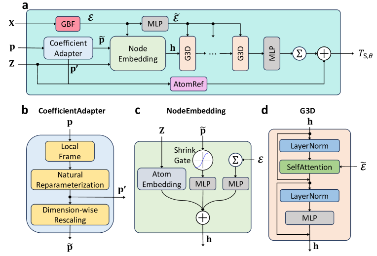
Figure 6: Overview of the KEDF model. (a) The KEDF model predicts the non-interacting kinetic energy (or a variant of it) from the given density, specified by the density coefficients $\mathbf{p}$, as well as the atomic numbers $\mathbf{Z}$ and coordinates $\mathbf{X}$ of atoms in the molecule that characterizes the atomic basis. A CoefficientAdapter module converts density coefficients $\mathbf{p}$ to $\mathrm{SE}(3)$-invariant density features $\tilde{\mathbf{p}}$. A NodeEmbedding module combines different feature sources and generates abstract atomic features $\mathbf{h}$, which are subsequently updated through a series of G3D layers. A GBF layer and a multi-layer perceptron (MLP) module produce pairwise distance features $\tilde{\bm{\mathcal{E}}}$ from coordinates $\mathbf{X}$, which are incorporated into each G3D layer to model atomic interactions. An MLP module converts the updated features into atomic energy, which is summed and then aggregated with the output of AtomRef to obtain the kinetic energy. (b) The CoefficientAdapter module consists of the LocalFrame module, followed by the other two enhancement modules: NaturalReparameterization and DimensionwiseRescaling. The LocalFrame module transforms the raw density coefficients $\mathbf{p}$ into $\mathrm{SE}(3)$-invariant density features $\tilde{\mathbf{p}}$, and the enhancement modules subsequently process the features to express a vast gradient range. The enhancement module of AtomRef covers the large gradient scale of the kinetic energy. (c) The NodeEmbedding module integrates information from three sources: atomic features obtained by an AtomEmbedding layer that assigns a learnable weight vector to each atom type (i.e., chemical element), density features processed by a ShrinkGate layer along with an MLP and aggregated GBF embeddings that encode chemical environment. (d) The G3D layer is the Graphormer layer based on the vanilla Transformer encoder layer, while uses the distance feature as an auxiliary attention bias.

Appendix B M-OFDFT Technical Details

In this section, we provide more technical details of the proposed M-OFDFT framework. We first provide a full description of the nonlocal neural network model to approximate the KEDF in Supplementary Sec. B.1. We then elaborate on other techniques to handle the unconventional challenges for learning a functional model, including the use of local frame to guarantee geometric invariance of the model in Supplementary Sec. B.2, and enhancement modules for expressing a large gradient range in Supplementary Sec. B.3. Furthermore, we discuss explorations on learning different density functional variants in Supplementary Sec. B.4. Finally, we detail the density optimization techniques in Supplementary Sec. B.5 with which M-OFDFT is used to solve a given molecular structure.

B.1 Model Specification

As motivated in the main paper, M-OFDFT utilizes the expansion coefficients $\mathbf{p}$ of the density under an atomic basis set as the direct density feature input into the functional model. Since the atomic basis depends on the molecular structure $\mathcal{M}$, the model also needs to include $\mathcal{M}$ into its input for a complete specification of the input density. Note that given $\mathbf{p}$ and $\mathcal{M}$, there is no need of explicit density gradient or Laplacian features since they are transmitted to the features of the basis functions and thus already embodied in $\mathcal{M}$. Compared to the grid-based representation, a common alternative for density representation, using the atomic-basis representation saves thousands of times the representation dimension. This is critical for implementing a nonlocal calculation in the model, which is well-known vital for approximating KEDF [22, 14, 8, 23, 21], but would otherwise be prohibited by the millions times more cost. The aggregation to atoms further reduces the required number of elements (nodes) in the nonlocal calculation. There are also works in the context of learning the XC functional that develop machine-learning models also using features under atomic basis [52, 53], but the models do not take the molecular structure in input and focus on processing the features hosted on each atom individually, hence are essentially not nonlocal models.

Although including $\mathcal{M}$ into the model input sacrifices formal universality, explicit dependency on $\mathcal{M}$ is arguably inevitable for an efficient density representation, which requires the structure of the problem, i.e., the pattern of the density (“inductive bias” in machine learning), to reduce the representation dimension. Even the irregular grid representation inherits the pattern of molecular structure, hence a nonlocal model using grid input feature still requires generalization across molecular systems. On the other hand, the nonlocal Graphormer model architecture, based on which our neural network model is designed, has shown attractive capability to generalize across conformations and chemicals for a range of molecular tasks in previous studies [33, 34, 63]. Our extrapolation study in Results 2.3 directly validates the superior generalization capability for OFDFT.

The KEDF model takes atomic numbers $\mathbf{Z}$, positions $\mathbf{X}$, and density coefficients $\mathbf{p}$ of all atoms in the molecule as input, which are then used to construct node features encoding information about the electron density surrounding each atom. These features are further transformed and employed to predict the non-interacting kinetic energy. The gradient of the KEDF w.r.t density coefficients for density optimization is obtained through auto-differentiation [92]. Considering the fact that nonlocal calculation is indispensable for KEDF, we build the nonlocal model based on the Graphormer architecture [33, 34]. Notably, Graphormer can handle varying-length input feature (as needed since different molecules have different numbers of atoms) in a permutation-invariant manner, which is not straightforward using other popular architectures such as multi-layer perceptions. The architecture has shown attractive performance in processing molecular structure to predict various properties, e.g., ground-state energy and HOMO-LUMO gap of molecular systems [33, 34], and also structure sampling from a thermodynamical ensemble [63]. The nonlocal architecture has an $O(N^{2})$ complexity, which does not increase the complexity of OFDFT.

An overview of the KEDF model is summarized in Supplementary Fig. 6(a). To adapt the Graphormer architecture for learning a physical functional, a few modifications are needed. The first new need is processing the input coefficients as a node (i.e., atom) feature, a NodeEmbedding layer is proposed to generate initial atomic representations from the coefficients it hosts, along with other input features. It uses a multi-layer perceptron (MLP) module to model the the intra-atomic density interaction (Supplementary Fig. 6(c)). Inter-atomic density-feature interaction is covered by the self-attention module in each Graphormer-3D (G3D) layer from [34]. Following the work, atom coordinates inputs are first converted to pairwise distances and are subsequently element-wise processed by the Gaussian basis function (GBF) layer, which expands each distance value, say $d_{ab}$, into an enriched distance feature vector $\bm{\mathcal{E}}_{ab}$ by evaluating on a series of Gaussian functions with learnable centers and scales. The pairwise distance features introduce a helpful pairwise feature into the attention module in the G3D layer (Supplementary Fig. 6(d)), which help identify the strength and ways of interactions between atomic features. They are also used to construct the initial node features through the NodeEmbedding layer (Supplementary Fig. 6(c)). Since the dependency of the output on the atomic coordinates $\mathbf{X}$ is only through the pairwise distances, the $\mathrm{SE}(3)$-invariance w.r.t $\mathbf{X}$ is naturally satisfied. The $\mathrm{SE}(3)$-invariance w.r.t the density coefficients $\mathbf{p}$ are guaranteed by the local frame technique in the CoefficientAdapter module (Supplementary Fig. 6(b)), which we will detail in Supplementary Sec. B.2. The natural reparameterization and dimension-wise rescaling modules in the CoefficientAdapter module, as well as the atomic reference (AtomRef) module are introduced to express large gradients, for which we detail in Supplementary Sec. B.3.

B.1.1 Atomic Basis Concatenation

As mentioned in Methods 4, M-OFDFT adopts atomic basis as an efficient density representation for molecules, which is especially important for constructing a nonlocal KEDF model. This saves thousands times the dimension of the density feature, which amounts to millions times of saving when conducting an explicit nonlocal calculation. Therefore, it enables a nonlocal KEDF model without much pain. We also note that atomic basis could also be used in material systems, so this way of density representation hence M-OFDFT is not restricted to non-periodic molecular systems.

Each basis function $\omega_{\mu}$ is specified by the position of the center atom and the basis function index, and we hence use $\mu=(a,\tau)$ to index the $\tau$-th basis function centered at atom $a$. The basis coefficients that can be attributed to each atom could naturally serve as node-wise density features for the molecule point-cloud. Specifically, an even-tempered basis set [65] with its $\beta$ parameter taken as $2.5$ is adopted as the density basis set (Eq. (110)). The number of basis in a molecule, $M$, is in the same order as the number of atoms $A$ or electrons $N$. Each atom type has its own set of basis functions and the size of each set $\mathcal{T}_{Z}$ varies from different atom types. The detailed orbital composition of each atom type is summarized in Supplementary Table 2. To make the coefficient vector homogeneous over all the atoms, these basis functions are concatenated and broadcast to all atoms, making a unified $\mathcal{T}$-dimensional density coefficient vector $\mathbf{p}_{a:}$ on any atom, where $\mathcal{T}:=\sum_{Z}\mathcal{T}_{Z}$ is the sum of basis functions over all considered atom types. In more detail, in the QM9 dataset, the 477-dimensional concatenated coefficient vector consists of 20, 109, 116, 116 and 116 basis functions which correspond to $\mathrm{H}$, $\mathrm{C}$, $\mathrm{N}$, $\mathrm{O}$ and $\mathrm{F}$, respectively. For example, given the coefficient of a hydrogen ($\mathrm{H}$) atom, we place them at the first 20 dimensions and use zero-valued vectors to mask other positions. A graphic illustration is shown in Supplementary Fig. 7. The zero-valued mask is also employed to mask the predicted gradient during density optimization, avoiding introducing irrelevant gradient information from masked positions.

Table 2: Orbital composition of basis set associated with each atom type.

Atom Type	Orbitals
$\mathrm{H}$	6s3p1d
$\mathrm{C}$	11s8p7d3f2g
$\mathrm{N}$	11s8p7d4f2g
$\mathrm{O}$	11s8p7d4f2g
$\mathrm{F}$	11s8p7d4f2g

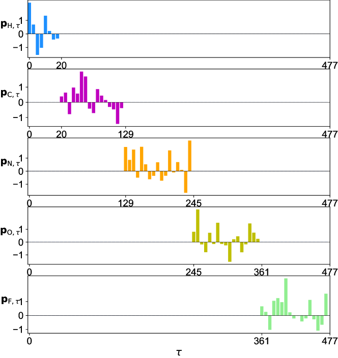
Figure 7: Concatenation of atomic basis for different atom types. $\tau$ is the index of density coefficient dimension and $\mathbf{p}_{Z,\tau}$ denotes the coefficient vector for atom aype $Z$. Note that this is a schematic illustration, so the coefficient dimensions may not correspond to the actual dimensions precisely.

B.1.2 NodeEmbedding Module

As shown in Supplementary Fig. 6(c), we design a NodeEmbedding module to integrate various input features into initial node representations $\mathbf{h}$, which are then passed to a neural network based on Graphormer to estimate the kinetic energy. Specifically, for atom $a$, an AtomEmbedding module generates atomic feature representation by assigning a learnable weight vector to the atom type $Z^{(a)}$. We also observed that the coefficient features $\tilde{\mathbf{p}}$ processed by the local frame technique in the CoefficientAdapter module exhibit a large numerical range, which is unfriendly for stable optimization in our practical trials. Thus, we apply a ShrinkGate layer $\lambda_{\rm co}\cdot\tanh(\lambda_{\rm mul}\,\tilde{\mathbf{p}})$ to map each density coefficient into a bounded space, where $\lambda_{\rm co}$ and $\lambda_{\rm mul}$ are learnable parameters. Due to the $\mathrm{SE}(3)$-invariant property of $\tilde{\mathbf{p}}$, applying any nonlinear operations (e.g., shrink function) on this feature will not violate the physical symmetry. After that, we use a MLP to further project the coefficient features into hidden density features. Following Graphormer [33], we embed the relative distance between two atoms with a set of Gaussian basis functions (GBF), where the mean and variance values of each basis are learnable parameters. To capture the chemical environment around atom $a$, we incorporate the aggregated GBF embedding $\sum_{b=1}^{A}\bm{\mathcal{E}}_{ab}$ as an auxiliary node feature. These three types of features are summed to form the initial node representations $\mathbf{h}_{a}\in\mathbb{R}^{D_{\rm hid}}$, where $D_{\rm hid}$ is the hidden dimension of the model.

B.1.3 Backbone Architecture

The neural network model in our KEDF model is built upon the Graphormer model, which is a Transformer-based graph neural network, and can efficiently perform global computation over the molecule structure while preserving the powerful expressiveness of the Transformer architecture. The model mainly consists of several stacked Graphormer-3D (G3D) layers, where each G3D layer is composed of an attention layer and a feed-forward layer (Supplementary Fig. 6(d)). The attention layer takes the hidden node representation $\mathbf{h}$ as the input tokens and uses the relative distance feature $\tilde{\bm{\mathcal{E}}}$ as a learnable attention bias for the attention mechanism. Specifically, given the node feature $\mathbf{h}=\{\mathbf{h}_{1},\cdots,\mathbf{h}_{A}\}$ and pairwise attention bias $\tilde{\bm{\mathcal{E}}}=\{\tilde{\bm{\mathcal{E}}}_{ab}\}_{a,b=1}^{A}$, where $a$ and $b$ denote the atom index, the G3D layer computes the attention score $\mathcal{A}_{ab}$ for one attention head as:

$$\mathcal{A}_{ab}=\frac{(\mathbf{h}_{a}\mathbf{U}^{(Q)})(\mathbf{h}_{b}\mathbf{U}^{(K)})^{\top}}{\sqrt{D^{\prime}_{\rm hid}}}+\tilde{\bm{\mathcal{E}}}_{ab},$$ (119)

where $\mathbf{U}^{(Q)}$ and $\mathbf{U}^{(K)}$ are the “query” and “key” linear projections for the node features and $D^{\prime}_{\rm hid}$ is the dimension of the query and key vectors in each attention head. To account for interactions between atom-centered electron density features, the GBF embedding $\bm{\mathcal{E}}$ is projected into pairwise attention bias $\tilde{\bm{\mathcal{E}}}$.

B.2 Local Frame Details for Geometric Invariance

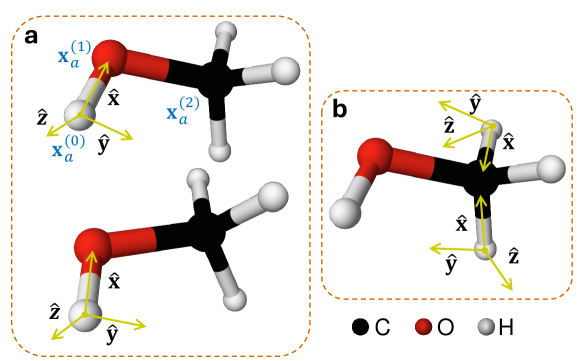
Figure 8: Illustration of the local frame. (a) The local frame is constructed for each atom according to its local environment, which is equivariant w.r.t. the transformation of the global frame. (b) Local frames of similar substructures (e.g., the three $\mathrm{H}$-$\mathrm{C}$ bonds in the methyl group) rotate with substructures accordingly, resulting in invariant coefficient features for locally similar density patterns.

As mentioned in Methods 4.2, by expanding the electron density on a set of atomic basis, the expansion coefficients $\mathbf{p}$ mathematically comprise geometric tensors of various orders equivariant to rotations and translations. A local frame simultaneously rotating with the structure is adopted to decouple the density feature from the change of the coordinate system and unnecessary geometric variability. As shown in Supplementary Fig. 8(a), to construct the local frame at an atom at $\mathbf{x}_{a}^{(0)}$, we choose $\hat{\mathbf{x}}$ pointing to its nearest atom $\mathbf{x}_{a}^{(1)}$. The $\hat{\mathbf{z}}$ axis lies in the line of the cross-product of $\hat{\mathbf{x}}$ with the direction to the second-nearest not-on-$\hat{\mathbf{x}}$ atom $\mathbf{x}_{a}^{(2)}$ and the $\hat{\mathbf{y}}$ axis is then given by $\hat{\mathbf{y}}=\hat{\mathbf{z}}\times\hat{\mathbf{x}}$. Note that we exclude the hydrogen atoms in the neighborhood of the center atom following [68], making the obtained local frame depend more on heavy atoms, whose positions are more stable than those of hydrogen atoms and reflect more reliable local structures. Denote the local frame associated with atom $a$ as:

$$\mathcal{R}_{a}:=(\hat{\mathbf{x}},\hat{\mathbf{y}},\hat{\mathbf{z}}),$$ (120)

the density coefficient vector and the gradient vector under the local frame are calculated by:

$$\mathbf{p}^{\prime l}_{a}=\mathbf{D}^{l}(\mathcal{R}_{a})\mathbf{p}^{l}_{a},\quad\nabla_{\mathbf{p}^{\prime l}_{a}}T_{\textnormal{S}}=\mathbf{D}^{l}(\mathcal{R}_{a})\nabla_{\mathbf{p}^{l}_{a}}T_{\textnormal{S}}.$$ (121)

where $l$ is the degree of tensors or azimuthal quantum number. $\mathbf{p}^{l}$ corresponds to the coefficient of basis functions of the degree $l$ (or type-$l$ tensors in mathematics). $\mathbf{D}^{l}(\mathcal{R}_{a})$ is the Wigner-D matrix of degree $l$.

Notably, an additional benefit of the local frame is that it makes a stable feature for locally similar density patterns. For example, consider the coefficients corresponding to the atomic basis on the three hydrogen atoms in a methyl group (Supplementary Fig. 8(b)). As the three $\mathrm{H}$-$\mathrm{C}$ bonds are highly indistinguishable, the densities on the bonds are very close and contribute almost identically to the kinetic energy. But as the three bonds have different orientations relative to a common global coordinate system, the coefficients on the hydrogen atoms are vastly different if the basis functions on different hydrogen atoms are aligned to the same directions. In contrast, basis functions under local frames are oriented equivariantly with the orientation of the local substructures, leaving the coefficients largely invariant, which makes more physical meanings to predict the energy. For example, coefficients on basis functions aligning with the $\hat{\mathbf{x}}$ direction always represent the density on the most significant (shortest) bond with the atom. As a result, the local frame makes almost the same density coefficients on the three hydrogen atoms in the methyl group even though the $\mathrm{H}$-$\mathrm{C}$ bonds have different orientations. We also provide a numerical visualization of the ethanol dataset, where the target functional is chosen as the residual energy of the non-interacting kinetic energy after deducted by the value given by the base kinetic energy functional APBE [41]. As shown in Supplementary Fig. 9, the local frame always attains a noticeable scale (standard deviation) reduction across various atom types, demonstrating its capability to eliminate unnecessary geometric variability caused by various orientations of the chemical bonds. More importantly, as shown in Supplementary Fig. 10, this approach also brings a significant scale reduction for gradient labels across various atom types, especially for $\mathrm{H}$ atoms, where almost all coefficient dimensions exhibit a $>$ 60% gradient scale reduction. This is crucial to alleviate the large gradient range and make the subsequent dimension-wise rescaling module easier (See more discussions in Supplementary Sec. B.3.1). These two advantages of the local frame are beneficial for the efficient optimization of the KEDF model. The empirical results in Supplementary Sec. D.4.3 suggest that the KEDF model achieves a 2-fold lower training and test error by using this technique.

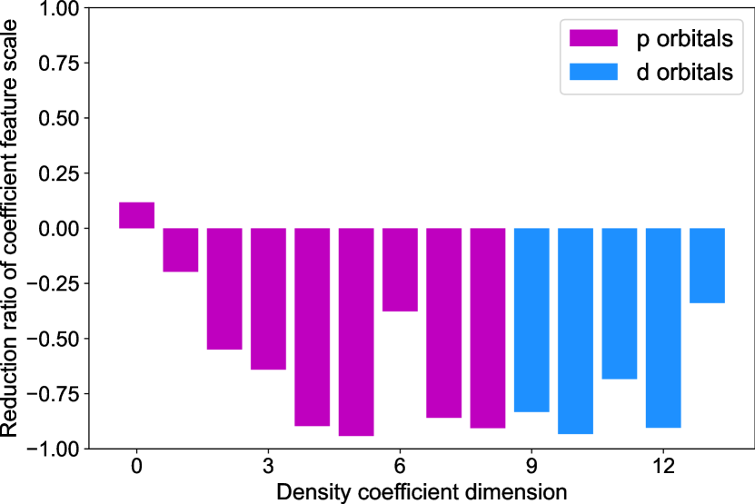
(a) H atom

(b) C atom

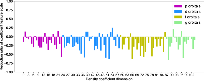
(c) N atom

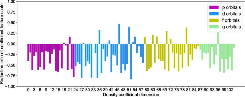
(d) O atom

Figure 9: Coefficient scale changes by the use of the local frame. For each coefficient dimension $\tau$ of atom type $Z$, the height of the bar represents the relative change in scale, calculated as $\frac{{\rm std\_coeff^{\prime}}_{Z,\tau}-{\rm std\_coeff}_{Z,\tau}}{{\rm std\_coeff}_{Z,\tau}}$, where ${\rm std\_coeff}_{Z,\tau}:=\mathrm{std}\{\mathbf{p}_{a,\tau}^{(d,k)}\}_{a:Z^{(a)}=Z,\;k,\,d}$ and ${\rm std\_coeff^{\prime}}_{Z,\tau}:=\mathrm{std}\{{\mathbf{p}^{\prime}}_{a,\tau}^{(d,k)}\}_{a:Z^{(a)}=Z,\;k,\,d}$ denote the coefficient scale before and after being transformed by the local frame, respectively. A negative value indicates a reduction in the scale of the coefficient due to the local frame transformation. Importantly, the local frame substantially decreases the coefficient scale across diverse basis dimensions and atom types.

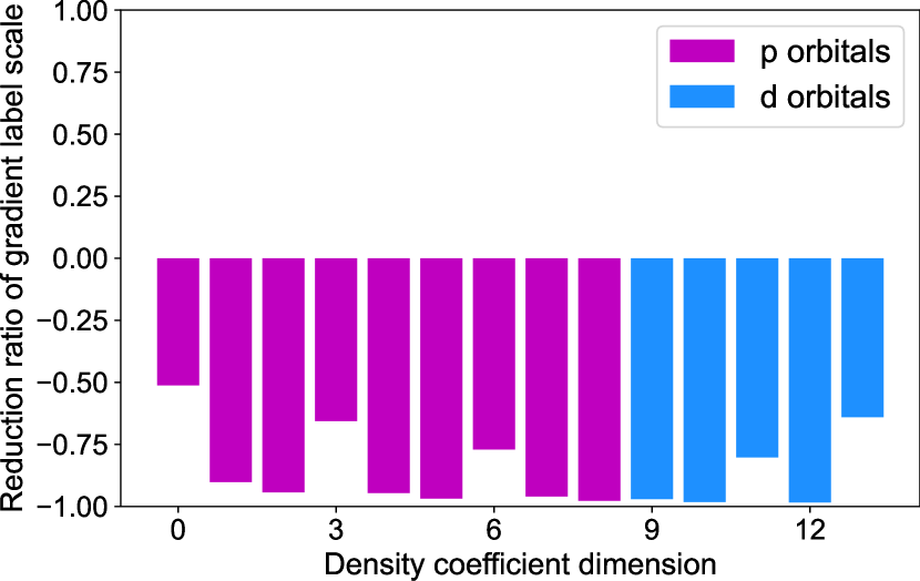
(a) H atom

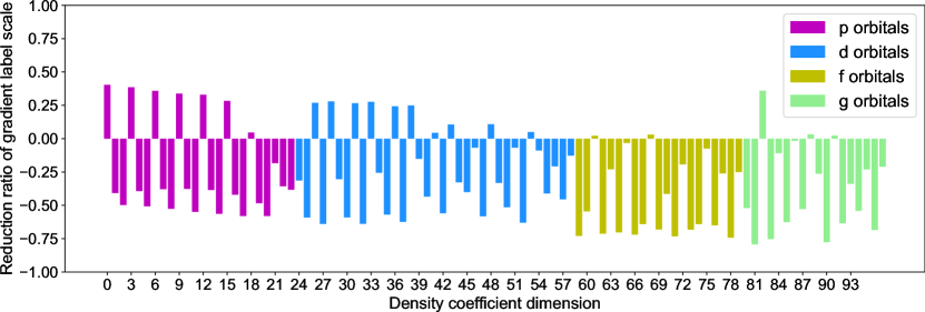
(b) C atom

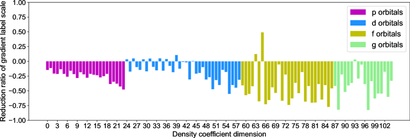
(c) N atom

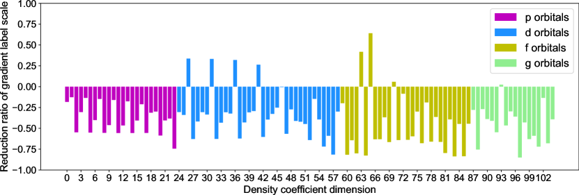
(d) O atom

Figure 10: Gradient scale changes by the use of the local frame. For each coefficient dimension $\tau$ of the atom type $Z$, the height of the bar represents the relative change in gradient scale, calculated as $\frac{\mathrm{max\_grad^{\prime}}_{Z,\tau}-\mathrm{max\_grad}_{Z,\tau}}{\mathrm{max\_grad}_{Z,\tau}}$, where $\mathrm{max\_grad}_{Z,\tau}:=\max\{\nabla_{\mathbf{p}_{a,\tau}}T_{\textnormal{S}}^{(d,k)}\}_{a:Z^{(a)}=Z,\;k,\,d}$ and $\mathrm{max\_grad^{\prime}}_{Z,\tau}:=\max\{\nabla_{\mathbf{p}_{a,\tau}}{T^{\prime}}_{\textnormal{S}}^{(d,k)}\}_{a:Z^{(a)}=Z,\;k,\,d}$ denote the gradient scale before and after being transformed by the local frame, respectively. The local frame transformation notably reduces the gradient scale across a wide range of basis dimensions and atom types.

B.3 Enhancement Modules Details for Expressing Vast Gradient Range

As mentioned in Methods 4.3, the raw gradient range of the input is vast, and conventional data normalization techniques are not applicable in our task since minimizing the gradient scale is conflicting with minimizing the coefficient scale. For the same reason we neither can take the logarithm of the density feature, as a number of works have adopted [97], since the gradient would be correspondingly scaled up. Another way to decrease the gradient scale is to downscale the energy value (i.e., using a larger energy unit). However, this does not bring further improvement in our trials. As mentioned in the main context, this is due to the trade-off between easy learning and model resolution: an error in the normalized (small) scale will be enlarged in the original scale. It neither works to use a separate model to learn the gradient directly, as we have empirically observed that the energy value model easily overfits the training data, and during density optimization the gradient model unnecessarily decreases the energy constructed from the value model and even appears non-conservative as the optimization diverges.

Having both large coefficients and gradients implies a function with a large Lipschitz coefficient, which leads to a great challenge for the optimization of conventional neural networks. According to these observations, we turn to elaborating on a series of enhancement modules to express the vast gradient range and enable effective training.

B.3.1 Dimension-wise Rescaling

Dimension-wise rescaling of coefficients and gradients is applied after the process of local frame and natural reparameterization. The two modules made the rescaling easier, but there is still a scale trade-off between coefficients and gradients. We hence choose moderate values for the scale parameters in Eq. (6): the target gradient scale $s_{\textnormal{grad}}$ is set to $0.05$ and the maximal coefficient scale $s_{\textnormal{coeff}}$ is set to $50$. Compared to the gradient scale, handling input coefficients with a larger range is more manageable. For example, incorporating a ShrinkGate module to further compress the coefficients into a bounded space, as discussed in Supplementary Sec. B.1.2. We found this technique yields an admirable performance empirically. Consequently, we prefer allowing a larger coefficient scale in the trade-off. In the context of deep learning, the Lipschitz coefficient (i.e., the maximum absolute gradient that the neural network model could express) is usually used to indicate the capability of a model fitting gradient label. Following this convention, we take the maximum absolute gradient value to measure the label scale.

To illustrate the importance of dimension-wise rescaling, we visualize the scales of gradients and density coefficients while learning residual KEDF on the QM9 dataset in Supplementary Fig. 11. The shown gradient scales are estimated after centralizing the gradient values by subtracting the gradient mean of each dimension with the atomic reference module. As plotted in Supplementary Fig. 11(a), many gradient dimensions have an extremely large scale. We found this leads to great difficulty in the practical optimization of deep learning models. After dimension-wise rescaling, most dimensions are rescaled to have the desired gradient scale (Supplementary Fig. 11(b)). As illustrated in Supplementary Fig. 11(c), the density coefficients are rescaled to a larger scale, and a ShrinkGate module is introduced to normalize the coefficients into a friendly space (Supplementary Sec. B.1.2). As a result, we found that the neural network model without the dimension-wise rescaling technique hardly converges and the loss curve is particularly volatile, due to the smoothness of common neural network architectures which restricts the range of the output gradient of the model. Applying the dimension-wise rescaling technique effectively mitigates this dilemma and enables efficient optimization.

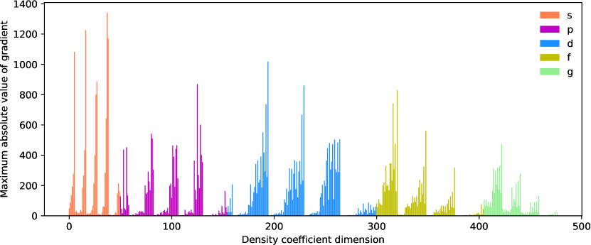
(a) Gradient scale of different coefficient dimensions (after processed by local frame and natural reparameterization, before dimension-wise rescaling).

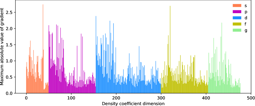
(b) Gradient scale after dimension-wise rescaling.

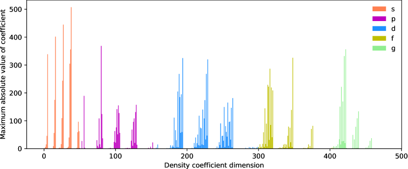
(c) Density coefficients scale after dimension-wise rescaling.

Figure 11: The gradient and density coefficient scale of QM9 dataset. The maximum absolute value is used to measure the maximum scale of data. (a)-(b) present the gradient scale before and after the dimension-wise rescaling transformation. This technique significantly reduces the gradient scale across various coefficient dimensions. (c) shows the corresponding coefficient scale after the dimension-wise rescaling transformation.

B.3.2 Natural Reparameterization

Although dimension-wise rescaling allows the trade-off between numerical scales of coefficients and gradients, the trade-off often has a difficult frontier that the two sides cannot be simultaneously made in a mild scale. A way to improve the trade-off is to balance the difficulties over the dimensions. The dimensions exhibit different scales since they have different sensitivity to the density hence the energy. Different basis functions spread over different regions in space, so a same amount of coefficient change on different basis functions influences the density function differently. To understand and balance the sensitivities, we derive how the change of coefficients affect the density function. Consider a small change $\Delta\mathbf{p}$ to the coefficients $\mathbf{p}$, which leads to a change in the density function $\Delta\rho(\mathbf{r}):=\rho_{\mathbf{p}+\Delta\mathbf{p}}(\mathbf{r})-\rho_{\mathbf{p}}(\mathbf{r})$. This difference is typically measured by the L2-metric in the function space: $\int\left\lvert\rho_{\mathbf{p}+\Delta\mathbf{p}}(\mathbf{r})-\rho_{\mathbf{p}}(\mathbf{r})\right\rvert^{2}\,\mathrm{d}\mathbf{r}=\int\left\lvert\Delta\rho(\mathbf{r})\right\rvert^{2}\,\mathrm{d}\mathbf{r}=\int\left\lvert\rho_{\Delta\mathbf{p}}(\mathbf{r})\right\rvert^{2}\,\mathrm{d}\mathbf{r}=\int\sum_{\mu}\Delta\mathbf{p}_{\mu}\omega_{\mu}(\mathbf{r})\sum_{\nu}\Delta\mathbf{p}_{\nu}\omega_{\nu}(\mathbf{r})\,\mathrm{d}\mathbf{r}=\Delta\mathbf{p}^{\top}\mathbf{W}\Delta\mathbf{p}$, where $\mathbf{W}_{\mu\nu}:=\int\omega_{\mu}(\mathbf{r})\omega_{\nu}(\mathbf{r})\,\mathrm{d}\mathbf{r}$ is the overlap matrix of the atomic basis for density. As the atomic basis is not orthonormal, $\mathbf{W}$ is not isotropic (i.e., cannot be turned proportional to the identity matrix by orthogonal transformations), so the same amount of coefficient change in different dimensions has different effects on the density function.

The proposed natural reparameterization $\tilde{\mathbf{p}}:=\mathbf{M}^{\top}\mathbf{p}$, where $\mathbf{M}$ is a square matrix satisfying $\mathbf{M}\mathbf{M}^{\top}=\mathbf{W}$, fulfills the desired balance. To see this, noting that $\mathbf{W}$ is non-singular hence is $\mathbf{M}$, we have $\mathbf{p}=\mathbf{M}^{-\top}\tilde{\mathbf{p}}$, so the density change is $\int\left\lvert\Delta\rho(\mathbf{r})\right\rvert^{2}\,\mathrm{d}\mathbf{r}=\Delta\mathbf{p}^{\top}\mathbf{W}\Delta\mathbf{p}=\Delta\tilde{\mathbf{p}}^{\top}\mathbf{M}^{-1}\mathbf{W}\mathbf{M}^{-\top}\Delta\tilde{\mathbf{p}}=\Delta\tilde{\mathbf{p}}^{\top}\mathbf{M}^{-1}\mathbf{M}\mathbf{M}^{\top}\mathbf{M}^{-\top}\Delta\tilde{\mathbf{p}}=\Delta\tilde{\mathbf{p}}^{\top}\Delta\tilde{\mathbf{p}}$, hence the change of coefficient in any dimension contributes equally to the density change. The gradient is reparameterized accordingly, following $\nabla_{\tilde{\mathbf{p}}}T_{\textnormal{S}}=(\nabla_{\tilde{\mathbf{p}}}\mathbf{p})^{\top}\nabla_{\mathbf{p}}T_{\textnormal{S}}=\mathbf{M}^{-1}\nabla_{\mathbf{p}}T_{\textnormal{S}}$.

Choosing the matrix $\mathbf{M}$ still faces a degree of freedom of an orthogonal transformation. We choose $\mathbf{M}=\mathbf{Q}\sqrt{\mathbf{\Lambda}}$, where $\sqrt{\mathbf{\Lambda}}$ denotes element-wise square-root operation, and the diagonal matrix $\mathbf{\Lambda}$ and orthogonal matrix $\mathbf{Q}$ come from the eigenvalue decomposition of $\mathbf{W}=\mathbf{Q}\mathbf{\Lambda}\mathbf{Q}^{\top}$ (note $\mathbf{W}$ is symmetric positive definite so such decomposition exists). We found it achieves more balanced sensitivity than using Cholesky decomposition in terms of the resulted largest gradient scale after dimension-wise rescaling. Although the eigenvalue decomposition requires a cubic complexity, it is only needed once per molecular structure, hence does not introduce a significant overhead compared to the cost in density optimization. Empirically, natural reparameterization considerably stabilizes the optimization of the functional model and brings lower training and validation loss, as presented in Supplementary Sec. D.4.3, underscoring the necessity of balancing the density coefficient with a physical metric.

B.3.3 Atomic Reference Module

The per-type bias statistics $\{\bar{T}_{Z}\}_{Z}$ and the global bias $\bar{T}_{\mathrm{global}}$ on the dataset are solved from the following over-determined linear equations using least squares method:

$$\bar{T}_{\mathcal{M}^{(d)}}:=\sum_{Z}A_{Z}^{(d)}\bar{T}_{Z}+\bar{T}_{\rm global}=\mathrm{mean}\{T_{\textnormal{S}}^{(d,k)}-{\bar{\mathbf{g}}_{\mathcal{M}^{(d)}}}^{\top}\mathbf{p}^{(d,k)}\}_{k},\quad\forall d,$$ (122)

where $A_{Z}^{(d)}:=\#\{a\in\mathcal{M}^{(d)}:Z^{(a)}=Z\}$ is the number of atoms of type $Z$ in molecule $\mathcal{M}^{(d)}$. Note that on the ethanol and Chignolin datasets where all structures share the same constitution, we only use the global bias, i.e., $\bar{T}_{\mathcal{M}}:=\bar{T}_{\rm global}$. A similar treatment for energy bias is also adopted in [75].

To demonstrate the benefit of the atomic reference module, we visualize the gradient scale reduction by the module on the QM9 dataset in Supplementary Fig. 12. We find that the atomic reference module significantly reduces the scale (variance) of gradient labels, especially for dimensions corresponding to ‘s’ atomic orbital functions. Since ‘s’ orbitals usually have large gradient mean values but small variance values, subtracting the gradient mean from these dimensions greatly simplifies the learning of gradient labels.

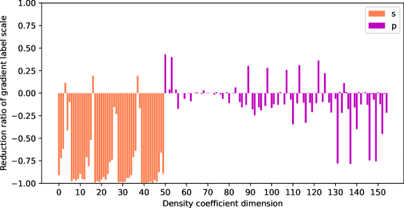
Figure 12: Gradient scale changes by the use of the atomic reference module. For coefficient dimension $\tau$ of the atom type $Z$, the height of the bar is also calculated by $\frac{\mathrm{max\_grad^{\prime}}_{Z,\tau}-\mathrm{max\_grad}_{Z,\tau}}{\mathrm{max\_grad}_{Z,\tau}}$, where $\mathrm{max\_grad}_{Z,\tau}:=\max\{\nabla_{\mathbf{p}_{a,\tau}}T_{\textnormal{S}}^{(d,k)}\}_{a:Z^{(a)}=Z,\;k,\,d}$ and $\mathrm{max\_grad^{\prime}}_{Z,\tau}:=\max\{\nabla_{\mathbf{p}_{a,\tau}}{T^{\prime}}_{\textnormal{S}}^{(d,k)}\}_{a:Z^{(a)}=Z,\;k,\,d}$ denote the gradient scale before and after being centralized by the atomic reference module, respectively. The atomic reference module considerably covers the vast gradient scale.

CoefficientAdapter Module

These enhancement modules and the neural network model are combined in the way shown in the model architecture Supplementary Fig. 6(a). In the architecture, the natural reparameterization module and the dimension-wise rescaling module are combined with the local frame technique into the CoefficientAdapter module (Supplementary Fig. 6(b)). It transforms the vanilla density coefficient $\mathbf{p}$ to a neural-network-friendly density feature $\tilde{\mathbf{p}}$ as the direct input to the neural network model. It not only guarantees geometric invariance of density features, but also facilitates efficient learning with vast gradient labels.

B.4 Functional Variants

In principle, besides the unknown KEDF, any energy density functionals in the decomposition formulation of ground-state energy (Eq. (19)) can be taken as the training objective of the proposed M-OFDFT framework. Here we first describe the two versions we mainly employed in the implementation of M-OFDFT, and then describe our exploration in other functional variants.

B.4.1 Residual KEDF

In the implementation of M-OFDFT, the first functional version we introduced aims to reduce the difficulty of modeling KEDF directly by employing an existing KEDF as the base functional and learning the residual:

$$T_{\textnormal{S},\theta}(\mathbf{p},\mathcal{M}):=T_{\textnormal{S,res},\theta}(\mathbf{p})+T_{\textnormal{S,base}}(\mathbf{p},\mathcal{M}).$$ (123)

Specifically, we chose the APBE KEDF [41] as the base KEDF since it best fits the training data on the QM9 dataset among four functionals mentioned in Supplementary Sec. C.3. Although the von Weizsäcker KEDF [43] provides a lower bound and could restrict the residual model to be positive, using it as a baseline introduces vast gradient labels for the residual that is hard to train.

B.4.2 TXC Functional

The residual KEDF version has achieved a simpler learning target with a tractable gradient range, but it has a computational bottleneck of evaluating the value and gradient of the APBE base KEDF as well as the PBE XC functional from the density coefficient, which is conducted through a grid. As discussed in Supplementary Sec. A.3.2, the time complexity of calculating the value is $O(MN_{\textnormal{grid}})$ (recall $M$ is the number of basis functions). Evaluating the gradient by automatic differentiation requires the same time complexity as evaluating the value, and moreover, it also requires $O(MN_{\textnormal{grid}})$ memory occupation to store intermediate values for back-propagation. Considering the large prefactor of $N_{\textnormal{grid}}$ (commonly $\sim 10^{3}N$), the computational cost for residual KEDF to conduct density optimization becomes unaffordable for large scale systems. Such cost was observed on the QMugs dataset. To get rid of calculation on grid, the second version of learning target for the deep-learning model is introduced as the sum of the KEDF and the XC functional, which we call the TXC functional, denoted as $E_{\textnormal{TXC},\theta}(\mathbf{p},\mathcal{M})$.

B.4.3 Learning Other Functionals

Besides the two versions above, we also experimented other direct targets for the deep-learning model to learn, including directly learning the KEDF $T_{\textnormal{S}}[\rho]$ (i.e., without a base KEDF), the universal functional $U[\rho]$ (Eq. (15)), and the total energy functional $E_{\textnormal{tot},\mathcal{M}}[\rho]$, i.e., electronic energy $E[\rho]$ in Eq. (19) plus inter-nuclear energy $E_{\textnormal{nuc}}(\mathcal{M})$ in Eq. (125) later. We found that both directly learning the KEDF and the universal functional are hard to optimize due to their large gradient range, which is even larger than that for learning the residual KEDF model and the TXC model, and cannot be effectively handled even using the proposed techniques. Interestingly, learning the total energy functional $E_{\textnormal{tot},\mathcal{M}}[\rho]$, i.e., adding the external energy $E_{\textnormal{ext}}$ and inter-nuclear energy $E_{\textnormal{nuc}}(\mathcal{M})$ to the universal functional as the target, significantly reduces the gradient range and enables stable optimization, especially on protein systems we considered. Specifically, on the 50 test Chignolin structures considered in Results 2.3, learning the total energy model $E_{\textnormal{tot},\theta}(\mathbf{p},\mathcal{M})$ using data of all peptides gives a better density optimization result (per-atom energy MAE 0.071$\,\mathrm{kcal/mol}$ as in Fig. 3(e) ‘M-OFDFT/Pretrain’, per-atom relative energy MAE 0.097$\,\mathrm{kcal/mol}$ as in Fig. 3(c) ‘M-OFDFT’) than learning the TXC model $E_{\textnormal{TXC},\theta}$ (per-atom energy MAE 0.102$\,\mathrm{kcal/mol}$, per-atom relative energy MAE 0.148$\,\mathrm{kcal/mol}$). Nevertheless, these results by the $E_{\textnormal{TXC},\theta}$ model are still reasonable and effective, and are significantly better than the classical OFDFT using the APBE KEDF (per-atom relative energy MAE 0.684$\,\mathrm{kcal/mol}$ as in Fig. 3(c) ‘APBE’).

B.5 Density Optimization Details

After a functional model is learned, M-OFDFT solves a given molecular structure by density optimization. Here we provide additional results and details for density optimization.

B.5.1 Additional Density Optimization Results

As mentioned in Methods 4.4, M-OFDFT can produce reasonable optimization curves for a given molecular structure from either of the two initialization methods Hückel and ProjMINAO, and gives accurate energy and HF force results. Here we provide more density optimization results in Supplementary Fig. 13 following the same setting as Fig. 5, except on a different QM9 molecule. First, we compare the optimization curves in energy by M-OFDFT and OFDFT with classical KEDFs including TF [4, 5], TF+$\frac{1}{9}$vW [12], TF+vW [42], and APBE [41], from the conventional MINAO [79] initialization. As illustrated in Supplementary Fig. 13(a-b), M-OFDFT converges closely to the true ground-state energy using both initialization methods, while all classical KEDFs lead to optimization curves falling below the true ground-state energy. We did not plot the curve for TF+$\frac{1}{9}$vW since it diverges so vastly that the curve soon runs out of the shown range.

We further plot the density error along with the optimization process, measured in the L2-metric $\int\left\lvert\rho(\mathbf{r})-\rho^{\star}(\mathbf{r})\right\rvert^{2}\,\mathrm{d}\mathbf{r}$ from the KSDFT ground-state density $\rho^{\star}(\mathbf{r})$ (see Supplementary Sec. B.3.2 for calculation details). As shown in Supplementary Fig. 13(c-d), M-OFDFT from either initialization continuously drives the density towards the true ground-state density and results in a small density error, even though the optimization process is not driven by minimizing the density error (but by minimizing electronic energy). This indicates that the energy objective of M-OFDFT constructed from the learned functional model is not artificial in the sense of only producing the correct energy after optimization, but it also leads to the correct electron density, so the functional holds the desired physical meaning. In contrast, density error curves by classical KEDFs diverge quickly and present an ascending trend, revealing a problem for applying these functionals to molecular systems. Again, we did not plot the curve for TF+$\frac{1}{9}$vW since it soon runs out of the shown range.

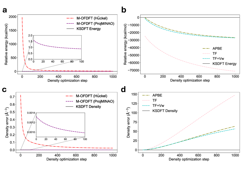
Figure 13: Density optimization curves by M-OFDFT and OFDFT with classical KEDFs. The figures come in parallel with Fig. 5 but on a different QM9 molecule. (a) Curves in relative energy along the density optimization process of M-OFDFT with different initialization methods. M-OFDFT converges closely to the true ground-state energy using either initialization method. (b) Curves in relative energy along the density optimization process of OFDFT using classical KEDFs. The curves run below the true ground-state energy with a significant gap. (c) Curves in density error along the density optimization process of M-OFDFT with different initialization methods. M-OFDFT converges closely to the true ground-state density using either initialization method, even though the optimization is not driven by minimizing the density error. (d) Curves in density error along the density optimization process of OFDFT using classical KEDFs. The curves diverge quickly. Curves for TF+$\frac{1}{9}$vW are omitted in (b) and (d) since they soon run out of the shown range.

B.5.2 Density Initialization Details

Recall that we introduced two initialization methods in Methods 4.4, Hückel and ProjMINAO, for stable density optimization in M-OFDFT. Initialization is worthy of the attention since it should stay in the training-data manifold of the functional model for reliable prediction. Training data come from eigensolutions of effective one-electron Hamiltonian matrix, which motivates the first choice of the Hückel initialization [80, 81] which follows the same mechanism. The second choice is to project the initial density onto the manifold, inspired by previous methods, e.g., using local PCA [24, 27] or kernel PCA [25]. But these existing projection techniques is not easily applicable for M-OFDFT since the density optimization domain is the coefficient space generated by the given molecular structure, which differs for different molecular structures, so it is not straightforward to determine the training-data manifold within the coefficient space for an unseen molecular structure. We hence use an additional deep-learning model to conduct the projection of the MINAO initialization, which we call ProjMINAO.

To implement the ProjMINAO initialization, we construct an additional output branch $\Delta\mathbf{p}_{\theta}(\mathbf{p},\mathcal{M})$ to predict the required correction to project the given density coefficient $\mathbf{p}$ towards the ground-state density coefficient $\mathbf{p}^{\star}$ for the molecular structure $\mathcal{M}$. Due to the formulation of KSDFT, the ground-state density corresponds to the eigensolution of an effective Hamiltonian (Supplementary Sec. A.2), hence is on the training-data manifold for sure. Projecting towards the ground state could also accelerate convergence in density optimization. The branch is built on top of the last G3D layer shown in Supplementary Fig. 6(a) of the KEDF model. It processes the hidden representations of each atom through an MLP module to predict the corresponding coefficient difference. The branch is trained to project the density coefficient data along the SCF iteration of KSDFT onto the corresponding ground-state coefficient:

$$\sum_{d}\sum_{k}\left\lVert\Delta\mathbf{p}_{\theta}(\mathbf{p}^{(d,k)},\mathcal{M}^{(d)})-(\mathbf{p}^{(d,k)}-\mathbf{p}^{(d,\star)})\right\rVert.$$ (124)

Note that even though the projection is aimed at the ground state, we do not rely on it for accuracy, as the functional model could continue optimizing the density (Fig. 5).

Since the MINAO or Hückel initialization primarily produces orbital coefficients, density fitting (Supplementary Sec. A.4.1) is required to convert them to density coefficients to complete the density initialization. Note that this procedure is performed only once for each molecular structure, so the cubic computational cost of density fitting (and generating Hückel initialized orbitals) does not dominate over the quadratic scaling of density optimization on regular workloads.

For very large molecules, we also propose an alternative initialization to directly generate the density coefficients by superposition of isolated-atom densities, in the same spirit of MINAO which uses the superposition of isolated-atom orbitals. This amounts to concatenating the fitted MINAO density coefficients of each atom as if in isolation, which only has a linear computational cost. This constructed density coefficients are then fed to the projection branch for the correction, which is the final initialized density. In practice, this technique drastically reduces the time needed to construct the initial coefficients, further reducing the overall time consumption of M-OFDFT, and renders only a minor increase of error (approximately 0.02$\,\mathrm{kcal/mol}$ in per-atom energy error on the interested protein systems in Results 2.4).

B.5.3 Stopping Criterion

Another required specification for density optimization is stopping criterion. Ideally, the solution from M-OFDFT is expected at the stationary point with zero projected gradient of the electronic energy. But in practice, the exact zero-gradient point may be missed due to discretization error. Therefore, we propose a set of stopping criteria to determine the practical stationary point over a chosen number of optimization steps.

• For molecules in a similar scale as those in training, the stopping criterion is chosen as the step with minimal single-step energy update, i.e., at the global (over the chosen number of optimization steps) minimum of single-step energy update. This is the closest step to the stationary point in practice.

• For larger-scale molecules than those in training, however, the above criterion is not as effective as on in-scale systems. The reason is that the reliable coefficient region around the ground-state density for the model is likely smaller and anisotropic due to the extrapolation risk, so the coefficients may find a mistaken direction to ”sneak off” the ground state in an extensive optimization. Note that it is hard to project the confronted density during optimization onto the training-data manifold precisely, since the manifold of coefficient is unknown for a molecular structure not present in training. Therefore, we mitigate this problem by controlling the extent of density optimization to balance optimization effectiveness and reliability. Specifically, we consider two additional criteria: (1) the step where the projected (onto the tangent space of normalized coefficients; not the training-data manifold) gradient norm first stops decreasing, i.e., the first local minimum of the projected gradient norm. (2) the step where the single-step energy first stops decreasing, i.e., the first local minimum of single-step energy update. These two criteria characterize a local minimum on the optimization process, hence represent a certain level of optimization effectiveness. Meanwhile, they are chosen to be the first encountered point with such characterization, where is likely still in the reliable region for the model. Based on empirical results on the validation set, we prefer first invoking criterion (1). If this criterion is not met within the chosen optimization steps, we seek for criterion (2). If this is still not met, we resort to the original criterion of the global minimum of single-step energy update, which always exists.

Appendix C Empirical Study Settings

C.1 Dataset Preparation

To substantiate the efficacy of the proposed method, we conduct evaluations on two distinct molecular datasets: ethanol and QM9. These datasets are specifically chosen to evaluate the generalization performance of M-OFDFT within both conformation space and chemical space. Furthermore, we seek to assess the extrapolation capability of M-OFDFT with larger molecular systems, for which two additional datasets are prepared: QMugs and Chignolin. Comprehensive supplementary information and generation details for each dataset are provided below.

C.1.1 Ethanol

To investigate the generalization ability of M-OFDFT in conformation space, we created a set of 100,000 non-equilibrium ethanol structures, randomly drawn from the MD17 dataset [37, 38]. These geometries were then randomly partitioned into training, validation and test sets using an 8:1:1 ratio.

C.1.2 QM9

The QM9 dataset [40] serves as a popular benchmark for predicting quantum-chemical properties using deep learning methods. It comprises equilibrium geometries of approximately 134k small organic molecules, composed of $\mathrm{H}$, $\mathrm{C}$, $\mathrm{O}$, $\mathrm{N}$, and $\mathrm{F}$ atoms. These molecules represent a subset of all species with up to nine heavy atoms from the GDB-17 chemical universe dataset [39]. As the dataset contains only equilibrium geometries, we employ it as a benchmark for evaluating the generalization ability of M-OFDFT in chemical space. Furthermore, to compare M-OFDFT with classical OFDFT methods, we include the 6905 isomers of $\mathrm{C_{7}H_{10}O_{2}}$ present in the QM9 dataset as a benchmark for assessing M-OFDFT in conformation space. We continue to randomly split the molecules into training, validation, and test sets using an 8:1:1 ratio.

C.1.3 QMugs

The QMugs dataset, proposed by Isert et al. [45], comprises over 665k biologically and pharmacologically relevant molecules extracted from the ChEMBL database, totaling approximately 2M conformers. Notably, QMugs provides molecular samples that are considerably larger than those in the QM9 and MD17 datasets, with an average of 30.6 and a maximum of 100 heavy atoms per compound. This allows us to study the extrapolation capabilities of M-OFDFT.

We group QMugs molecules based on the number of heavy atoms into bins with a width of 5, except for the first bin, which contains molecules with 10-15 heavy atoms. To construct an extrapolation task, we divide the union of QM9 and the first QMugs bin into training and validation sets with a 9:1 ratio, and test M-OFDFT on 50 molecular structures from each of the other bins with increasing scales. The results are shown in Fig. 3(a).

For the extrapolation setting in Fig. 3(b) for investigating the amount of additional larger-scale molecular data required by end-to-end counterparts M-PES and M-PES-Den to achieve a comparable extrapolation performance as M-OFDFT, the target workload of large molecules is fixed, while the affordable training datasets contain increasingly larger molecules. Specifically, taking the QM9 dataset as the base data source, the molecular structures from the first four QMugs bins are progressively incorporated to build four training datasets. All training datasets are prepared with the same size to eliminate statistical effects, while the composition ratio of each data source is designed to follow their relative composition ratios in the original joint dataset (QM9 $\cup$ QMugs), as presented in Supplementary Fig. 14.

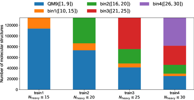
Figure 14: Compositions of training datasets from QM9 and QMugs for the extrapolation setting in Fig. 3(b). The training datasets contain the same number of data points (molecular structures), while involve increasingly larger molecules. The proportion of molecules in each scale range (i.e., QM9, bin1-bin4) respects the proportion in the joint dataset. The range of the number of heavy atoms in each data source is listed in the figure (i.e., $[1,9]$ for QM9).

C.1.4 Chignolin

Data Selection

To further evaluate the extrapolation ability of M-OFDFT on large-scale biomolecular molecules, such as proteins, we sampled 1,000 Chignolin structures from an extensive molecular dynamic (MD) simulation [48]. Due to its fast-folding property and short length (TYR-TYR-ASP-PRO-GLU-THR-GLY-THR-TRP-TYR), Chignolin has been widely used in molecular dynamics studies. Following Wang et al. [98], we first featurized the backbone conformations into all pairwise $\alpha$-carbon-atom distances, excluding pairs of nearest neighbor residues. Then, a time-lagged independent component analysis (TICA) [99, 100] was conducted with a lag time of $\tau_{\rm lag}=20$ ns, projecting the conformations onto a low-dimensional subspace. The first eight TICA components were clustered into 1,000 groups using the $k$-means algorithm. The centroid structure of each cluster was extracted using MDTraj [101] and taken as the representative structure.

Conformation Neutralization

In this study, we focus on isolated molecular systems where all atoms or functional groups stay neutral and all electrons are paired. However, protein molecules extracted from MD trajectories are simulated in aqueous solution and some of its functional groups are ionized, such as the amine group in the N-terminal and the carboxyl group in the C-terminal. In our setting, we neutralize protein conformations by editing (adding/deleting) hydrogen atoms in ionizable groups using OpenMM [102], which is expected to have a minimal impact on the original geometry. The hydrogen definition template was modified to handle hydrogen atoms not defined in standard amino acids, such as the missing hydrogen atom in the carboxyl group in the C-terminal amino acid. We then performed local energy optimization on the neutralized conformations using Amber [103], with the Amber-ff14SB force field and a maximum of 100 optimization cycles. To prevent significant geometry changes, we only allowed hydrogen atoms associated with heavy atoms involved in the hydrogen editing process to be optimized. For neutralized amino acids without standard force field templates, we built force field parameters using the antechamber and parmchk2 tools in Amber.

Protein Fragmentation

To investigate the extrapolation utility of M-OFDFT from “local” fragments to “global” proteins, we created our datasets by cutting each of the 1,000 Chignolin structures into protein fragments (i.e., polypeptides) of varying lengths. To construct these fragments, we enumerated all possible polypeptides with sequence lengths up to five in the Chignolin sequence. Specifically, we allow fragments of length 5 to be composed of two dipeptides or a dipeptide and a tripeptide, i.e., dipeptide-[GAP]-dipeptide and tripeptide-[GAP]-dipeptide. The extracted fragment molecules were capped with hydrogen atoms instead of larger capping groups to minimize the introduction of significant geometry changes. These fragments were then used as training and validation sets with a 9:1 ratio. It should be noted that when benchmarking the performance of deep-learning methods trained with different molecule scales, the training set with a maximum peptide length of $L_{\rm pep}$ is comprised of all polypeptides with sequence lengths less than $L_{\rm pep}$.

For the comparison of M-OFDFT with classical KEDFs in Fig. 3(c), we only used 50 Chignolin structures as the test set, since classical KEDFs require grid-based quadrature which is very costly for running on all the 1,000 Chignolin structures.

Data Filtration

After preliminary analysis, we found that the range of energy and gradient labels in fragments datasets are too vast to fit even if equipped with several efficient training techniques (see Supplementary Sec. B.3). Moreover, most of the vast data points come from the first several steps of the SCF iterations that are far from convergent. To mitigate this issue, we filter out data points if the residual between its energy and the ground-state energy is larger than 500$\,\mathrm{kcal/mol}$. This strategy can empirically improve the optimization robustness and prediction performance.

C.2 Data Generation Configurations

KSDFT Calculations

All KSDFT calculations were carried out using the PySCF [79] software package, which is open-sourced and has a convenient Python interface that allows flexible customization, e.g., for implementing the data generation process detailed in Supplementary Sec. A.4, and implementing M-OFDFT calculation described in Results 2.1 using automatic differentiation packages in Python. A well-acknowledged pure XC functional (i.e., only depends on density but not orbitals), e.g., PBE [93], is used to make sure the data pairs demonstrate a density functional. Restricted-spin calculation and the 6-31G(2df,p) basis set were adopted, which is sufficient for the considered molecules which are uncharged, in near-stable conformations, and only involve light atoms (up to fluorine). To accelerate the calculations, density fitting with the def2-universal-jfit [106] basis set was enabled in the calculations for molecules with more than 30 atoms. Grid level was set to 2. Convergence tolerence was set to 1 $\mathrm{meV}$. Slight modifications to the PySCF code were made to log the required information (e.g., the molecular orbitals) for SCF intermediate steps. Direct Inversion in Iterative Subspace (DIIS) was enabled, following the defaults. Per-molecule statistics such as running time and number of atoms were collected alongside the calculation for benchmarking purposes.

KSDFT Initialization

The MINAO initialization method is employed to conduct KSDFT calculation for data generation, adhering to the default settings. We would like to mention that as explained and empirically shown in Methods 4.4, the Hückel initialization achieves a good convergence behavior for density optimization of M-OFDFT, since it comes from an eigenvalue-problem solution hence aligns with the way how the training data are generated (Supplementary Sec. A.4). It is then motivated to generate data also using the Hückel initialization for running KSDFT, in hope to further align the training data with the use cases (i.e., density optimization of M-OFDFT using Hückel initialization), making the use cases lie more in-distribution with the training data and expecting better density optimization results. We tried generating and leveraging such data, but found the generated data entries from different SCF iterations on the same molecular structure show much larger variance, especially the gradient labels. This brings more challenges on training stability and effectiveness, which are hard to handle effectively even with the techniques in Methods 4.3 and Supplementary Sec. B.3. Although using Hückel-initialized data improves the accuracy of Hückel-initialized M-OFDFT on ethanol, the improvement is not obvious on QM9, and using Hückel-initialized data does not improve the accuracy of ProjMINAO-initialized M-OFDFT on either dataset, due to that the training challenges outweigh the benefits.

Hardware Details

All KSDFT calculations and preprocessing (e.g., density fitting) procedures were carried out on a cluster of 700 capable CPU servers. Each server in the cluster has 256 GiB of memory and 32 Intel Xeon Platinum 8272CL cores with hyperthreading disabled.

Dataset Preprocessing

After the SCF runs, extra procedures were done to transform the SCF results into datasets for training and evaluation. The density coefficients were obtained using the density fitting procedure detailed in Supplementary Sec. A.4.1, with the auxiliary basis set being an even-tempered basis set [65] generated on-the-fly with $\beta=2.5$ (see Eq. (110)). After that, gradient and force labels were calculated using the obtained density coefficients following Supplementary Sec. A.4.3 and C.5. Energy labels were calculated following Supplementary Sec. A.4.2. For large orbital integrals in the procedure, proper symmetries in the atomic orbital indices were leveraged to save computation and reduce memory footprint. Local frame transformation and natural reparameterization (detailed in Supplementary Sec. B.2 and Supplementary Sec. B.3.2) were applied to the coefficients to obtain the model inputs.

C.3 Classical OFDFT Methods Implementation

To benchmark the advantages of M-OFDFT, we select several classical kinetic energy density functionals (KEDFs) for reference. The Thomas-Fermi (TF) KEDF [4, 5] $T_{\textnormal{TF}}[\rho]:=\frac{3}{10}(3\pi^{2})^{\frac{2}{3}}\int\rho(\mathbf{r})^{5/3}\mathrm{d}\mathbf{r}$ is exact in the uniform electron gas limit. The von Weizsäcker KEDF [43] takes the form $T_{\textnormal{vW}}[\rho]:=\frac{1}{8}\int\frac{\left\lVert\nabla\rho(\mathbf{r})\right\rVert^{2}}{\rho(\mathbf{r})}\mathrm{d}\mathbf{r}$, which is exact for bosons and a single fermion (or electron pair). When expanding KEDF up to the first-order derivatives of the density at the uniform density limit, the result is $T_{\textnormal{TF}}[\rho]+\frac{1}{9}T_{\textnormal{vW}}[\rho]$ [12]. We also include a variant of this correction $T_{\textnormal{TF}}[\rho]+T_{\textnormal{vW}}[\rho]$, which is also considered in [42]. The base APBE KEDF [41] is also tested. For a fair comparison, these functionals are implemented in the same framework as M-OFDFT. Similar to the way we use the PBE XC functional and the ABPE KEDF as mentioned in Supplementary Sec. A.3.2, we also re-implemented the TF, TF+$\frac{1}{9}$vW, and TF+vW functionals in PySCF using Pytorch. Their values are evaluated by numerical quadrature on a grid in the 3-dimensional space. To solve for the ground-state density, gradient descent is used, for which the gradient of the kinetic energy is directly evaluated by automatic differentiation. The same stopping criterion is used. For initialization, we use the MINAO method, which we found better than the Hückel method. It is worth noting that classical OFDFT methods depend on computationally intensive grid calculations, making the evaluation cost prohibitive for large molecular systems.

We also attempted to use other state-of-the-art OFDFT software for comparison, such as PROFESS [107], GPAW [108], ATLAS [109] and DFTpy [110]. However, most of them are tailored for periodic material systems and depend heavily on sophisticated pseudopotentials that are not pure or multiplicative. Adapting these codes to molecular systems of our interest is challenging since they only provide local pseudopotentials for a few main group elements, which do not cover the atom types ($\mathrm{H}\mathrm{C}\mathrm{N}\mathrm{O}\mathrm{F}$) we are interested in, and we encountered difficulties in generating reliable pseudopotentials for these atom types. Although GPAW can handle molecular systems, we found that its OFDFT calculations on molecular systems are hard to converge even for small molecules with default settings and looser convergence criterion.

C.4 M-PES and M-PES-Den Implementation

Results 2.3 demonstrate that M-OFDFT has the ability to extrapolate to large molecular systems, a valuable advantage for quantum chemistry methods. We measure the significance of this advantage by contrasting M-OFDFT with two deep-learning-based alternatives, M-PES and M-PES-Den, that are aimed to predict the total energy (ground-state electronic energy plus inter-nuclear energy) from the molecular structure $\mathcal{M}$. Both alternatives employ the same Graphormer backbone architecture as M-OFDFT, but they do not have the density projection branch (Supplementary Sec. B.5.2), and M-PES does not have the density coefficient input branch in its NodeEmbedding module (Supplementary Fig. 6(c)). The model hyperparameters are also adjusted to be comparable to those of M-OFDFT.

C.5 Hellmann-Feynman Force Calculation

To more comprehensively evaluate M-OFDFT, we also employ the Hellmann-Feynman (HF) force [111, 112] as a metric to evaluate the results of M-OFDFT. The force experienced by atoms in a molecule is itself an important quantity as it is directly required for geometry optimization and molecular dynamics simulation. The HF force is a simple way to estimate the force, and is exact in the limit of complete basis. Due to the simplicity, the HF force can also be seen as an evaluation of the optimized density.

Hellmann-Feynman Force

Force is the negative gradient of the total energy of a molecule as a function $E_{\textnormal{tot}}(\mathbf{X})$ of atom coordinates $\mathbf{X}=\{\mathbf{x}^{(a)}\}_{a=1}^{A}$ (molecular conformation). We omit the dependency on the molecular composition $\mathbf{Z}$ for brevity. The total energy $E_{\textnormal{tot}}(\mathbf{X}):=E^{\star}_{\mathbf{X}}+E_{\textnormal{nuc}}(\mathbf{X})$ comprises both the electronic energy $E^{\star}_{\mathbf{X}}$ in electronic ground state (including interaction with the nuclei), and also the energy from inter-nuclear interaction:

$$E_{\textnormal{nuc}}(\mathbf{X}):=\frac{1}{2}\sum_{\begin{subarray}{c}a,b=1,\cdots,A,\\ a\neq b\end{subarray}}\frac{Z^{(a)}Z^{(b)}}{\lVert\mathbf{x}^{(a)}-\mathbf{x}^{(b)}\rVert},$$ (125)

which gives the inter-nuclear part of the force,

$$-\nabla_{\mathbf{x}^{(a)}}E_{\textnormal{nuc}}(\mathbf{X})=-Z^{(a)}\sum_{b:\neq a}Z^{(b)}\frac{\mathbf{x}^{(b)}-\mathbf{x}^{(a)}}{\lVert\mathbf{x}^{(b)}-\mathbf{x}^{(a)}\rVert^{3}}.$$ (126)

The electronic energy $E^{\star}_{\mathbf{X}}$ is the minimum after a variational optimization process for solving the electronic ground state of the molecule in conformation $\mathbf{X}$. In the most fundamental form, $E^{\star}_{\mathbf{X}}$ is determined by the variational problem on $N$-electron wavefunctions as shown in Eq. (9). The Hamiltonian operator therein $\hat{H}_{\mathbf{X}}=\hat{T}+\hat{V}_{\textnormal{ee}}+\hat{V}_{\textnormal{ext},\mathbf{X}}$ depends on the conformation $\mathbf{X}$ through $V_{\textnormal{ext},\mathbf{X}}$, which is given in Eq. (10). The ground-state wavefunction $\psi^{\star}_{\mathbf{X}}$ and energy $E^{\star}_{\mathbf{X}}=\langle\psi^{\star}_{\mathbf{X}}|\hat{H}_{\mathbf{X}}|\psi^{\star}_{\mathbf{X}}\rangle$ hence also depend on $\mathbf{X}$. The gradient of $E^{\star}_{\mathbf{X}}$ can then be reformed as: $\nabla_{\mathbf{X}}E^{\star}_{\mathbf{X}}=$

$$\nabla_{\mathbf{X}}\langle\psi^{\star}_{\mathbf{X}}|\hat{H}_{\mathbf{X}}|\psi^{\star}_{\mathbf{X}}\rangle =\langle\nabla_{\mathbf{X}}\psi^{\star}_{\mathbf{X}}|\hat{H}_{\mathbf{X}}|\psi^{\star}_{\mathbf{X}}\rangle+\langle\psi^{\star}_{\mathbf{X}}|\nabla_{\mathbf{X}}\hat{H}_{\mathbf{X}}|\psi^{\star}_{\mathbf{X}}\rangle+\langle\psi^{\star}_{\mathbf{X}}|\hat{H}_{\mathbf{X}}|\nabla_{\mathbf{X}}\psi^{\star}_{\mathbf{X}}\rangle$$ (127)

$$\stackrel{{\scriptstyle\text{(*)}}}{{=}}E^{\star}_{\mathbf{X}}\langle\nabla_{\mathbf{X}}\psi^{\star}_{\mathbf{X}}|\psi^{\star}_{\mathbf{X}}\rangle+\langle\psi^{\star}_{\mathbf{X}}|\nabla_{\mathbf{X}}\hat{H}_{\mathbf{X}}|\psi^{\star}_{\mathbf{X}}\rangle+E^{\star}_{\mathbf{X}}\langle\psi^{\star}_{\mathbf{X}}|\nabla_{\mathbf{X}}\psi^{\star}_{\mathbf{X}}\rangle$$ (128)

$$=\langle\psi^{\star}_{\mathbf{X}}|\nabla_{\mathbf{X}}\hat{H}_{\mathbf{X}}|\psi^{\star}_{\mathbf{X}}\rangle+E^{\star}_{\mathbf{X}}\nabla_{\mathbf{X}}\langle\psi^{\star}_{\mathbf{X}}|\psi^{\star}_{\mathbf{X}}\rangle$$ (129)

$$\stackrel{{\scriptstyle\text{(\#)}}}{{=}}\langle\psi^{\star}_{\mathbf{X}}|\nabla_{\mathbf{X}}\hat{H}_{\mathbf{X}}|\psi^{\star}_{\mathbf{X}}\rangle,$$ (130)

where the equality (*) is due to that $\psi^{\star}_{\mathbf{X}}$ is an eigenstate of the Hermitian operator $\hat{H}_{\mathbf{X}}$ with real eigenvalue $E^{\star}_{\mathbf{X}}$, and the equality (#) is due to that the wavefunction is normalized $\langle\psi^{\star}_{\mathbf{X}}|\psi^{\star}_{\mathbf{X}}\rangle=1$ for all $\mathbf{X}$. Eq. (130) is the Hellmann-Feynman (HF) theorem [111, 112]. To continue the calculation, the gradient of the Hamiltonian operator in the expression can be derived as $\nabla_{\mathbf{x}^{(a)}}\hat{H}_{\mathbf{X}}=\nabla_{\mathbf{x}^{(a)}}\hat{V}_{\textnormal{ext},\mathbf{X}}$, and by noting that $\hat{V}_{\textnormal{ext},\mathbf{X}}$ is multiplicative and one-body as shown in Eq. (10), we have $\nabla_{\mathbf{x}^{(a)}}V_{\textnormal{ext},\mathbf{X}}(\mathbf{r})=-Z^{(a)}\frac{\mathbf{r}-\mathbf{x}^{(a)}}{\lVert\mathbf{r}-\mathbf{x}^{(a)}\rVert^{3}}$, and subsequently, the electronic force can be calculated as:

$$-\nabla_{\mathbf{x}^{(a)}}E^{\star}_{\mathbf{X}}=-\langle\psi^{\star}_{\mathbf{X}}|\nabla_{\mathbf{x}^{(a)}}\hat{H}_{\mathbf{X}}|\psi^{\star}_{\mathbf{X}}\rangle=Z^{(a)}\int\rho^{\star}_{\mathbf{X}}(\mathbf{r})\frac{\mathbf{r}-\mathbf{x}^{(a)}}{\lVert\mathbf{r}-\mathbf{x}^{(a)}\rVert^{3}}\,\mathrm{d}\mathbf{r}=:\mathbf{f}^{(a)}_{\mathbf{X}},$$ (131)

where $\rho^{\star}_{\mathbf{X}}(\mathbf{r}):=\rho_{[\psi^{\star}_{\mathbf{X}}]}(\mathbf{r})$ defined in Eq. (11). This is the Hellmann-Feynman (HF) force $\mathbf{f}_{\mathbf{X}}$. This expression coincides with the electrostatic force under a classical view, indicating “there are no ‘mysterious quantum-mechanical forces’ acting in molecules” [84]. From the expression, evaluating the HF force only requires a good approximation to the ground-state electronic density $\rho^{\star}_{\mathbf{X}}(\mathbf{r})$, which is available in various quantum chemistry methods, including $\rho_{\mathbf{C}^{\star}_{\mathbf{X}}}$ in KSDFT given by Eq. (52) and $\rho_{\mathbf{p}^{\star}_{\mathbf{X}}}$ in M-OFDFT given by Eq. (47). The total force on the nuclei is the sum with the inter-nuclear force in Eq. (126).

Analytical Force

However, when using the atomic basis, there emerges approximation error in the function representation, since the basis is incomplete. Consequently, the conditions of the HF theorem do not hold exactly. This makes the HF force in Eq. (131) only an approximation to the true electronic force $-\nabla_{\mathbf{x}^{(a)}}E^{\star}_{\mathbf{X}}$, and other approximations are possible. For example, $-\nabla_{\mathbf{x}^{(a)}}E^{\star}_{\mathbf{X}}$ can also be estimated by directly taking the analytical gradient of the electronic energy $E^{\star}_{\mathbf{X}}$ expressed under the atomic basis with the optimal coefficients [113]. This way of estimating the electronic force is hence called analytical force $\mathbf{f}_{\textnormal{ana},\mathbf{X}}$. For KSDFT, $E^{\star}_{\mathbf{X}}=E_{\mathbf{X}}(\mathbf{C}^{\star}_{\mathbf{X}})$, where $E_{\mathbf{X}}(\mathbf{C})$ is given by Eqs. (62-66) (note that the basis functions $\eta_{\alpha}$, $\eta_{\beta}$ and matrices $\mathbf{T}$, $\tilde{\mathbf{D}}$ and $\mathbf{V}_{\textnormal{ext}}$ all depend on $\mathbf{X}$), and $\mathbf{C}^{\star}_{\mathbf{X}}$ is the optimal orbital coefficients. The corresponding analytical force on an atom $a$ can be expanded as:

$$\mathbf{f}^{(a)}_{\textnormal{ana},\mathbf{X}}:=-\nabla_{\mathbf{x}^{(a)}}E_{\mathbf{X}}(\mathbf{C}^{\star}_{\mathbf{X}})=-(\nabla_{\mathbf{x}^{(a)}}E_{\mathbf{X}})(\mathbf{C}^{\star}_{\mathbf{X}})-\operatorname{tr}\Big{(}(\nabla_{\mathbf{x}^{(a)}}\mathbf{C}^{\star}_{\mathbf{X}})^{\top}\nabla_{\mathbf{C}}E_{\mathbf{X}}(\mathbf{C})\Big{|}_{\mathbf{C}=\mathbf{C}^{\star}_{\mathbf{X}}}\Big{)},$$ (132)

where $(\nabla_{\mathbf{x}^{(a)}}E_{\mathbf{X}})$ takes the gradient with a fixed $\mathbf{C}$, and $\nabla_{\mathbf{x}^{(a)}}\mathbf{C}^{\star}_{\mathbf{X}}$ is the Jacobian, $(\nabla_{\mathbf{x}^{(a)}}\mathbf{C}^{\star}_{\mathbf{X}})_{\alpha i,\xi}:=\partial(\mathbf{C}^{\star}_{\mathbf{X}})_{\alpha i}/\partial\mathbf{x}^{(a)}_{\xi}$ in which $\xi\in\{1,2,3\}$ indices the three spacial components, and matrix operations, including transpose, matrix multiplication and trace, act on indices $\alpha$ and $i$. When $\mathbf{C}^{\star}_{\mathbf{X}}$ is indeed accurately optimized, self-consistency in Eq. (71) and orthonormality in Eq. (67) are satisfied. By also noting Eq. (70), the second term in Eq. (132) vanishes: $\operatorname{tr}\big{(}(\nabla_{\mathbf{x}^{(a)}}\mathbf{C}^{\star}_{\mathbf{X}})^{\top}\nabla_{\mathbf{C}}E_{\mathbf{X}}(\mathbf{C})\big{|}_{\mathbf{C}=\mathbf{C}^{\star}_{\mathbf{X}}}\big{)}\stackrel{{\scriptstyle\text{Eq.~{}\eqref{eqn:grad-and-fock}}}}{{=}}2\operatorname{tr}\big{(}(\nabla_{\mathbf{x}^{(a)}}\mathbf{C}^{\star}_{\mathbf{X}})^{\top}\mathbf{F}_{\mathbf{C}^{\star}_{\mathbf{X}}}\mathbf{C}^{\star}_{\mathbf{X}}\big{)}\stackrel{{\scriptstyle\text{Eq.~{}\eqref{eqn:ksdft-scf-converged}}}}{{=}}2\operatorname{tr}\big{(}(\nabla_{\mathbf{x}^{(a)}}\mathbf{C}^{\star}_{\mathbf{X}})^{\top}\mathbf{S}_{\mathbf{X}}\mathbf{C}^{\star}_{\mathbf{X}}\bm{\upvarepsilon}^{\star}_{\mathbf{X}}\big{)}=\operatorname{tr}\Big{(}(\nabla_{\mathbf{x}^{(a)}}\mathbf{C}^{\star}_{\mathbf{X}})^{\top}\nabla_{\mathbf{C}^{\star}_{\mathbf{X}}}\operatorname{tr}\big{(}({\mathbf{C}^{\star}_{\mathbf{X}}}^{\top}\mathbf{S}_{\mathbf{X}}\mathbf{C}^{\star}_{\mathbf{X}}-\mathbf{I})\bm{\upvarepsilon}^{\star}_{\mathbf{X}}\big{)}\Big{)}=\nabla_{\mathbf{x}^{(a)}}\operatorname{tr}\big{(}({\mathbf{C}^{\star}_{\mathbf{X}}}^{\top}\mathbf{S}_{\mathbf{X}}\mathbf{C}^{\star}_{\mathbf{X}}-\mathbf{I})\bm{\upvarepsilon}^{\star}_{\mathbf{X}}\big{)}\stackrel{{\scriptstyle\text{Eq.~{}\eqref{eqn:coeff-orb-orthon}}}}{{=}}0$. If in practice $\mathbf{C}^{\star}_{\mathbf{X}}$ is not exactly optimized, the contribution from $\nabla_{\mathbf{x}^{(a)}}\mathbf{C}^{\star}_{\mathbf{X}}$ should also be considered; see Pulay [113] for detailed treatments.

Note that only the $-(\nabla_{\mathbf{x}^{(a)}}\bar{\mathbf{V}}_{\textnormal{ext},\mathbf{X}})^{\top}\bar{\mathbf{\Gamma}}^{\star}_{\mathbf{X}}$ term ($\bar{\mathbf{\Gamma}}^{\star}_{\mathbf{X}}$ is the vector of flattened optimal density matrix $\mathbf{\Gamma}^{\star}_{\mathbf{X}}:=\mathbf{C}^{\star}_{\mathbf{X}}{\mathbf{C}^{\star}_{\mathbf{X}}}^{\top}$), as a part of $-(\nabla_{\mathbf{x}^{(a)}}E_{\mathbf{X}})(\mathbf{C}^{\star}_{\mathbf{X}})$, corresponds to the HF force (see Eq. (66)). Other terms in the analytical force $\mathbf{f}^{(a)}_{\textnormal{ana},\mathbf{X}}$ in Eq. (132) are collectively called the Pulay force after [113], i.e., $\mathbf{f}_{\textnormal{ana},\mathbf{X}}-\mathbf{f}_{\mathbf{X}}$. They come in the form of the gradient of the basis functions w.r.t atom coordinates, hence are non-zero when using atomic basis and differentiate the analytical force from the HF force.

Implementation

Although the analytical force is regarded as a more accurate estimation when using atomic basis, we still take the HF force to evaluate the results, since the way to calculate the analytical force is different for different methods: KSDFT and M-OFDFT require different types of Coulomb integrals under different basis sets, and M-PES and M-PES-Den only require back-propagating the gradient through the deep-learning model. Moreover, the HF force in Eq. (131) only depends on the density from the ground-state solution, so it can also be seen as a relevant metric to evaluate the solved density.

For each molecular system, we take the true value of HF force as that given by the KSDFT solution, where the density is taken after density fitting (see Supplementary Sec. A.4.1). The HF force by M-OFDFT is calculated directly from the optimized density. For M-PES and M-PES-Den, as they cannot provide the density, only the corresponding analytical forces, $-\nabla_{\mathbf{X}}E_{\textnormal{tot},\theta}(\mathbf{X})$ and $-\nabla_{\mathbf{X}}E_{\textnormal{tot},\theta}(\mathbf{X},\mathbf{p}^{\textnormal{init}})$, are available. Note that since they predict the total energy, the inter-nuclear force $-\nabla_{\mathbf{X}}E_{\textnormal{nuc}}(\mathbf{X})$ (Eq. (126)) is included in the gradients. To convert them into HF forces, we extract from the gradients with the inter-nuclear force as well as the Pulay force: $\mathbf{f}_{\textnormal{M-PES},\mathbf{X}}^{(a)}=-\nabla_{\mathbf{x}^{(a)}}E_{\textnormal{tot},\theta}(\mathbf{X})-(-\nabla_{\mathbf{x}^{(a)}}E_{\textnormal{nuc}}(\mathbf{X}))-(\mathbf{f}_{\textnormal{ana},\mathbf{X}}^{(a)}-\mathbf{f}^{(a)}_{\mathbf{X}})$, and similarly for $\mathbf{f}_{\textnormal{M-PES-Den},\mathbf{X}}^{(a)}$, where the analytical force $\mathbf{f}_{\textnormal{ana},\mathbf{X}}^{(a)}$ and the HF force $\mathbf{f}^{(a)}_{\mathbf{X}}$ are calculated from KSDFT. Following previous works [37, 114], the error in predicted force is measured by the mean absolute error (MAE) over each of the three spacial components of the force on each atom in each molecule in the test set.

C.6 Curve Fitting Details

For fitting the curves in Fig. 3(a) and Fig. 4, we restrict the formulas $(\mathtt{a}N_{\mathrm{heavy}}+\mathtt{b})^{\mathtt{c}}+\mathtt{d}$ of all curves in each figure to have the same scale, i.e., the same $\mathtt{a}$. Otherwise, the flexibility of $\mathtt{a}$ would diminish the reflection of the exponent $\mathtt{c}$ on the curvature of the curve on the provided range of $N_{\mathrm{heavy}}$ (i.e., a smaller $\mathtt{a}$ allows a larger exponent $\mathtt{c}$). We found that sharing the same $\mathbf{a}$ in different curves hardly hinders the closeness to fitted data points. A two-phase fitting strategy is put forward based on this idea: (1) we jointly fit all curves with a shared $\mathtt{a}$, obtaining the pre-optimized $\mathtt{a}^{\prime}$; (2) taking $\mathtt{a}^{\prime}$ as an initial guess, we re-fit all curves independently to obtain the post-optimized $\mathtt{a}^{*}$ using the Trust Region Reflective optimization algorithm [115], where we restrict the search space of variable $\mathtt{a}$ into $[\mathtt{a}^{\prime}(1-\xi),\mathtt{a}^{\prime}(1+\xi)]$, with $\xi=0.5$. The two-phase fitting strategy approximately keeps all post-optimized $\mathtt{a}^{*}$ in the same scale as well as bring better fitting accuracy. The fitting process is conducted using the SciPy [116] package in Python.

C.7 Hyperparameter Configurations

C.7.1 Model Configuration

In all experimental settings, we employ the same backbone architecture, Graphormer, specifically utilizing the Graphormer-3D (G3D) encoder layer. To ensure a fair comparison, most hyperparameters in all models are maintained consistently (e.g., model depth and hidden dimension). A summary of all hyperparameter choices can be found in Supplementary Table 3. It is worth mentioning that in the shrink gate of NodeEmbedding, the initial value of learnable parameters $\nu_{\rm co}$ is set to 10, while the initial value of $\nu_{\rm mul}$ is set to 0.02 for the ethanol dataset and 0.05 for all other datasets. We did not conduct an extensive hyperparameter search, and most hyperparameters were chosen following Graphormer [33]. All models are implemented using the Pytorch deep learning framework [92].

Table 3: Hyperparameters of the Graphormer model used in all methods (M-OFDFT, M-PES, M-PES-Den).

Hyperparameter	M-OFDFT
G3D Layers	12
Hidden Dimension	768
Feed-Forward Hidden Dimension	768
Number of Heads	32
GBF Dimension	128
Dropout	0.1
Attention Dropout	0.1
Optimizer	Adam
Learning Rate Schedule	Linear decay
Adam ($\beta_{1},\,\beta_{2}$)	(0.95, 0.99)
Adam $\epsilon$	$1\times 10^{-8}$

C.7.2 Training Hyperparameters

Following Graphormer [33], all models are trained using the Adam optimizer and a linear decay learning schedule. The peak learning rate is set to $1\times 10^{-4}$ for our functional models and $3\times 10^{-4}$ for baseline models (i.e., M-PES and M-PES-Den). Other optimizer hyperparameters can be found in Supplementary Table 3. A warmup stage featuring a linearly increasing learning rate is introduced to stabilize training during the initial stage. The number of warmup steps is set to 30k for M-OFDFT and 60k for baseline models. The batch size is set to 256 for the ethanol dataset and 128 for all other datasets. All models are trained on Nvidia Tesla V100 GPUs.

For different molecule datasets, the number of training epochs is determined by examining the loss curve. Training is halted once the validation loss fails to decrease for 20 epochs. Specifically, our functional models are trained for approximately 600 and 700 epochs on the ethanol and QM9 datasets, respectively. For the QMugs dataset, our model is trained for approximately 700 epochs, while the M-PES and M-PES-Den models are trained for 2,300 epochs. Notably, we propose a series of QMugs datasets with increasing molecular size in Results 2.3, where the number of SCF data points will slightly increase as the average molecular size increases (larger molecules generally require more SCF iterations to converge). To ensure a fair comparison, we maintain approximately the same number of training epochs for different datasets. In the Chignolin experiment, there are four Chignolin datasets with increasing peptide length and data size. Our functional models are trained for 1,400, 1,100, 800, and 750 epochs, respectively, while the M-PES and M-PES-Den models are trained for 3,000, 3,000, 1,000, and 900 epochs, respectively.

In practice, we employ a weighted loss function to optimize the KEDF model:

$$L=\xi_{\rm eng}L_{\rm eng}+\xi_{\rm grad}L_{\rm grad}+\xi_{\rm den}L_{\rm den},$$ (133)

where $L_{\rm eng}$, $L_{\rm grad}$, and $L_{\rm den}$ represent the KEDF energy loss (Eq. (4)), gradient loss (Eq. (5)), and projected density loss (Eq. (124)), respectively. $\xi_{\rm eng}$, $\xi_{\rm grad}$, and $\xi_{\rm den}$ are the corresponding loss weights. The selection of loss weights is determined through grid search on the validation set for various datasets independently, and the utilized loss weights are provided in Supplementary Table 4.

Table 4: Loss weights for various datasets and learning targets.

Dataset	$\xi_{\rm eng}$	$\xi_{\rm grad}$	$\xi_{\rm den}$
Ethanol-$T_{\textnormal{S,res}}$	1	0.1	0.08
Ethanol-$E_{\textnormal{TXC}}$	1	0.03	1
QM9-$T_{\textnormal{S,res}}$	1	0.12	0.005
QM9-$E_{\textnormal{TXC}}$	1	0.12	0.05
QMugs	1	0.1	1
Chignolin	1	0.1	1

C.7.3 Density Optimization Hyperparameters

During the deployment stage, we use the ProjMINAO as the initialization choice for all settings in Results 2. The adopted gradient descent steps and step size $\varepsilon$ are chosen according to the performance of evaluation datasets. The gradient descent steps and step size are set to 1000 and $1\times 10^{-3}$ for all molecular datasets and functional variants (including traditional KEDF baselines), with the exception of implementing the learned KEDF models $T_{\textnormal{S,res},\theta}$ and $E_{\textnormal{TXC},\theta}$ on the ethanol dataset, where the step size $\varepsilon$ is set to $5\times 10^{-4}$. The vanilla Stochastic Gradient Descent (SGD) optimizer is adopted in the density optimization process.

Appendix D Additional Empirical Results

D.1 In-Scale Results

D.1.1 Quantitative Results

Table 5: Performance of M-OFDFT with different learning targets and initialization configurations, as an extension to the results narrated in Results 2.2. The mean absolute errors (MAEs) in energy and Hellmann-Feynman (HF) force are listed in $\mathrm{kcal/mol}$ and $\mathrm{kcal/mol/\text{\r{A}}}$, respectively.

Method	Ethanol		QM9
	Energy	HF force	Energy	HF force
$T_{\textnormal{S,res}}$-Hückel	5.27	27.73	9.88	12.73
$T_{\textnormal{S,res}}$-ProjMINAO	0.18	1.18	0.93	2.91
$E_{\textnormal{TXC}}$-Hückel	3.95	126.65	9.69	123.51
$E_{\textnormal{TXC}}$-ProjMINAO	0.18	2.07	0.73	4.73
M-PES	0.10	25.24	0.25	7.72

As mentioned in Results 2.2, M-OFDFT achieves chemical accuracy on unseen conformations (ethanol) and chemicals (QM9) in a similar scale as seen during training, using a deep-learning model targeting the residual KEDF on top of a base KEDF. Here we provide results under more technical choices in Supplementary Table 5. Firstly, we let the model learn the sum of the kinetic and XC energy $E_{\textnormal{TXC}}$ to get rid of the large prefactor of grid computation for calculation on large-scale molecules (Supplementary Sec. B.4.2). This is adopted in time complexity (Results 2.4) and extrapolation (Results 2.3) studies, and here we list its performance in this in-scale case. Secondly, as presented in Methods 4.4, two initialization strategies are proposed to address the out-of-distribution issue of initialized density. The results reported in Results 2.2 are produced by ProjMINAO initialization, and here we also list the results produced by the Hückel initialization method, which is one of the standard initialization methods in common DFT calculation [79, 81], and does not require an additional deep-learning model (or module). We also provide the results of M-PES, i.e., a deep-learning model with the same architecture that directly predicts the ground-state energy of the given molecular structure in an end-to-end way.

From Supplementary Table 5, we can see that although the $E_{\textnormal{TXC}}$ model combines with an additional unknown density functional, it can still be effectively trained, and does not have obvious negative effects on the accuracy. The energy accuracy is even improved on both datasets given the same initialization method. For the initialization methods, even without the deep-learning shortcut, M-OFDFT still achieves a reasonable accuracy using the Hückel initialization. With an additional deep-learning module for predicting a correction, the ProjMINAO initialized density stays close to the ground-state density, so it can yield better results. Finally, M-OFDFT achieves a comparable energy accuracy with the end-to-end method M-PES, even though the process to give the energy by M-OFDFT (density optimization using the KEDF model) is not directly supervised. Notably, on tasks that do not have a direct supervision, M-OFDFT is superior over M-PES. As the table shows, M-OFDFT achieves a significantly more accurate HF force estimation than M-PES, even though neither has seen HF force label in training. Abundant evidence in Results 2.3 also shows the dominating advantage of M-OFDFT in extrapolation to molecules larger than seen during training.

D.1.2 Visualization of Optimized Densities

For more qualitative investigation of M-OFDFT, we provide more visualization results of the optimized density by M-OFDFT, in addition to Fig. 2(b). Supplementary Fig. 15 shows the radial density by spherical integral around the other two heavy atoms in the ethanol molecule, i.e., the $\alpha$-carbon atom (the one connected to the oxygen atom) and the $\beta$-carbon atom. The results demonstrate that the density curves of M-OFDFT again align almost identically with the KSDFT density curves. In contrast, the classical KEDF using APBE for KEDF again leads to a substantial deviation around bonding regions between peaks of core electrons.

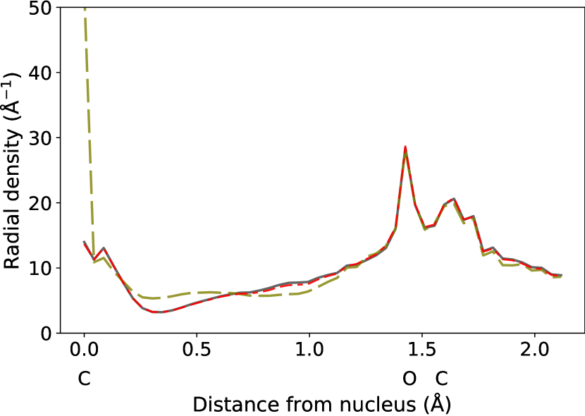
(a) $\alpha$-carbon

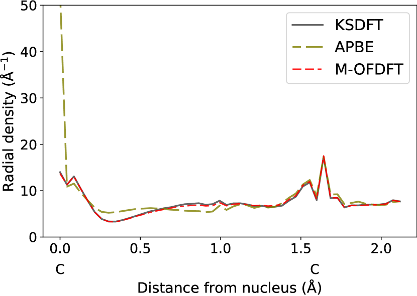
(b) $\beta$-carbon

Figure 15: Additional visualization of the density optimized by various methods. Integrated density on spheres of varying radii around each of the two carbon atoms in an ethanol structure is plotted in each figure, in parallel with Fig. 2(b).

D.2 Extrapolation Results

As shown in Results 2.3, M-OFDFT has shown a superior extrapolation performance in energy than end-to-end deep-learning counterparts M-PES and M-PES-Den that predict the total energy directly. We emphasize here that this is not due to that M-PES and M-PES-Den are not well trained or overfit to the training dataset. Supplementary Table 6 shows that M-PES and M-PES-Den achieve a better validation error than M-OFDFT, but their extrapolation errors increase much more vastly than that of M-OFDFT.

We further show the better extrapolation performance of M-OFDFT in HF force. As shown in Supplementary Fig. 16(a), M-OFDFT with functional model trained on molecules with fewer than 15 heavy atoms consistently maintains a significantly lower HF force MAE than M-PES and M-PES-Den on larger-scale molecules. M-OFDFT also outperforms the two end-to-end counterparts across various fragment datasets in the Chignolin experiment (Supplementary Fig. 16(b)).

In the finetuning setting of Chignolin, Supplementary Fig. 16(c) shows that M-OFDFT always achieves much better HF force results than M-PES and M-PES-Den in each of the three setups. M-OFDFT attains a significant 40.8% HF force error reduction in finetuning over training from scratch, showing the ability of capturing transferable knowledge from accessible-scale data, and more efficiently leveraging limited large-scale data. In contrast, the end-to-end deep-learning methods exhibit even worse HF force results when incorporating accessible-scale data, manifesting an extrapolation difficulty to a larger scale.

Table 6: Training, validation and extrapolation error (per-atom energy MAE in $\mathrm{kcal/mol}$) of our M-OFDFT and reference methods M-PES and M-PES-Den on the QMugs and Chignolin extrapolation setups. For the QMugs case, all the methods are trained and validated on two disjoint splits of QM9 molecules and QMugs molecules with no more than 15 heavy atoms, and are tested for extrapolation on 50 QMugs molecular structures with 56-60 heavy atoms. For the Chignolin case, all the methods are trained and validated on two disjoint splits of fragment structures of all peptide lengths (2-5), and are tested for extrapolation on 1,000 Chignolin structures. Note that for M-OFDFT, the training and validation energy errors are from end-to-end model output, while the extrapolation error is from the result after density optimization using the model, consistent with Fig. 3.

Method	QMugs			Chignolin
	Train	Validation	Extrapolation	Train	Validation	Extrapolation
M-PES	0.008	0.017	1.768	0.003	0.003	0.084
M-PES-Den	0.004	0.019	1.824	0.002	0.002	0.079
M-OFDFT	0.044	0.055	0.112	0.015	0.016	0.071

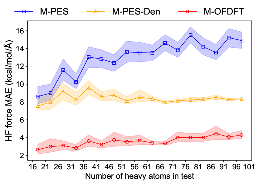
(a) QMugs (fixed training dataset, in parallel with Fig. 3(a))

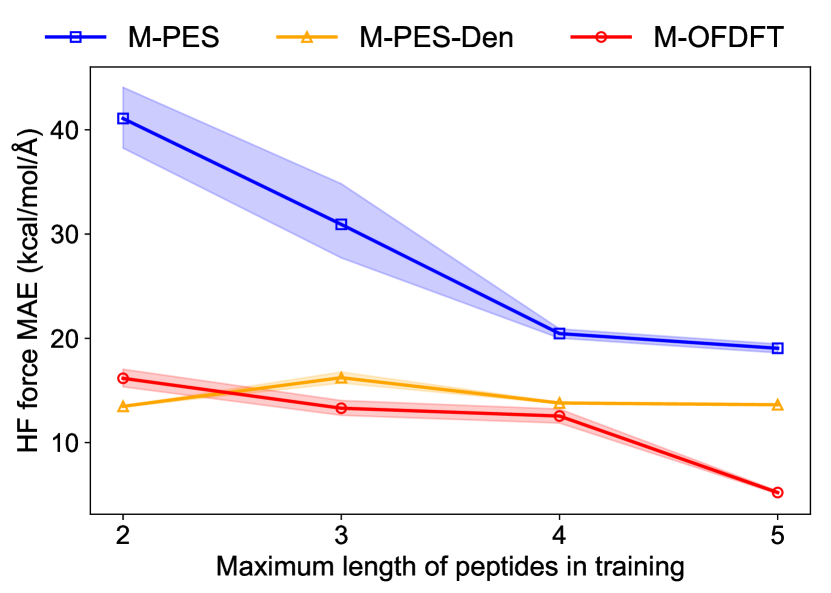
(b) Chignolin (fixed test dataset, in parallel with Fig. 3(d))

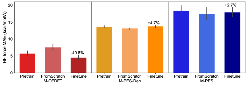
(c) Chignolin (finetuning setting, in parallel with Fig. 3(e))

Figure 16: Extrapolation performance in HF force of M-OFDFT compared with M-PES and M-PES-Den on the two extrapolation settings. (a) HF force MAE on increasingly larger molecules from the QMugs dataset, using models trained on molecules with no more than 15 heavy atoms from QM9 and QMugs datasets, in parallel with Fig. 3(a). (b) HF force MAE on 1,000 Chignolin structures, using models trained on a series of datasets including increasingly longer peptides, in parallel with Fig. 3(d). (c) HF force MAE on 50 Chignolin structures, using models trained on all peptides without (‘Pretrain’) and with ‘Finetune’ on 500 Chignolin structures, in parallel with Fig. 3(e). Also marked are error reduction ratios by the finetuned models over models trained ‘FromScratch’ on the 500 Chignolin structures only.

D.3 Empirical Time Cost Results

As mentioned in Results 2.4, we aim to demonstrate the lower time complexity of M-OFDFT compared to KSDFT by empirically benchmarking the two methods on two types of large molecular systems. For KSDFT calculations on all systems, we adopt the same settings as introduced in Supplementary Sec. C.2. For large QMugs molecules, we apply the learned TXC functional model $E_{\textnormal{TXC},\theta}$ in the same setting as used to produce Fig. 4. To further highlight the scaling advantage of M-OFDFT, we evaluate it on two large-scale protein molecular systems containing 709 and 738 atoms. The all-atom conformations of these systems are obtained from Lindorff-Larsen et al. [48] and neutralized following the same pipeline for processing Chignolin structures (detailed in Supplementary Sec. C.1.4). Such a scale is already seldom encountered in the context of KSDFT calculations. Considering the substantial scale difference between the protein systems evaluated and the molecules used during training, we employ the total energy functional model $E_{\textnormal{tot},\theta}(\mathbf{p},\mathcal{M})$ trained on all Chignolin fragments and finetuned on 800 Chignolin structures. This model is expected to provide the best extrapolation capacity within our available resources.

The results indicate that M-OFDFT achieves a 25.6-fold and 27.4-fold speedup over KSDFT on the two protein systems, respectively. The per-atom energy MAE of M-OFDFT on the two test systems is 0.23$\,\mathrm{kcal/mol}$ and 0.31$\,\mathrm{kcal/mol}$, respectively. While higher than the error on the Chignolin case, the result still demonstrates a significant advantage over M-PES, which gives per-atom energy MAE of 0.36$\,\mathrm{kcal/mol}$ and 0.63$\,\mathrm{kcal/mol}$, respectively.

D.4 Ablation Study

D.4.1 Multi-Step Data and Gradient Label

To capture the energy landscape in the density coefficient space, we generate multiple $\mathbf{p}$ samples for each molecular structure $\mathcal{M}$ and compute the gradient label $\nabla_{\mathbf{p}}T_{\textnormal{S}}$ for additional supervision information. An ablation experiment is conducted on the ethanol dataset to investigate the significance of each type of supervision by excluding the supervision label during the training process. The ablation results are presented in Supplementary Table 7. We observe that removing the gradient label $\nabla_{\mathbf{p}}T_{\textnormal{S}}$ leads to a considerable decrease in energy and HF force accuracy for both density initialization strategies, emphasizing the importance of maintaining the optimization of M-OFDFT on a physical track. Incorporating multi-step $\mathbf{p}$ samples is also crucial for enhancing the performance of M-OFDFT, particularly for the ProjMINAO initialization, as the accuracy of the density corrector model depends on the size of training densities.

Table 7: Ablation study for various data augmentation strategies. All results are evaluated on test ethanol molecules with the learned $T_{\textnormal{S,res},\theta}$ model. The MAEs in energy and HF force are listed in $\mathrm{kcal/mol}$ and $\mathrm{kcal/mol/\text{\r{A}}}$, respectively.

Multi-step $\mathbf{p}$	Gradient $\nabla_{\mathbf{p}}T_{\textnormal{S}}$	Density Initialization	Energy	HF Force
✓	✓	Hückel	5.27	27.73
		ProjMINAO	0.18	1.18
✓		Hückel	166.84	144.78
		ProjMINAO	170.83	143.67
	✓	Hückel	6.43	32.83
		ProjMINAO	20.61	38.56

D.4.2 Nonlocality

Considering the nonlocal dependency of KEDF on electron density, it is essential to incorporate nonlocal calculations in OFDFT, which motivates us to use Graphormer as our backbone architecture. To demonstrate the importance of nonlocality, we conduct an ablation study by gradually decreasing the receptive field (i.e., the distance cutoff of atom neighborhood) of the functional model (specifically, the TXC model (Supplementary Sec. B.4.2)) of M-OFDFT. The experiment follows the extrapolation setting in parallel with Supplementary Table 6, i.e., the functional model is trained on molecules with no more than 15 heavy atoms and the resulting M-OFDFT is tested on 50 QMugs molecular structures with 56-60 heavy atoms. As illustrated in Supplementary Fig. 17, both the energy and HF force prediction error tend to worsen as the distance cutoff decreases, providing empirical evidence in our setting that a nonlocal model is indeed indispensable for well approximating a functional involving the kinetic energy density functional (KEDF).

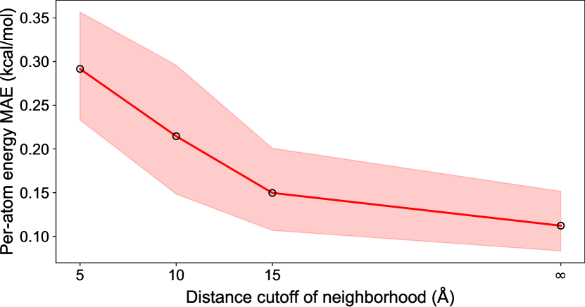
(a) Energy results

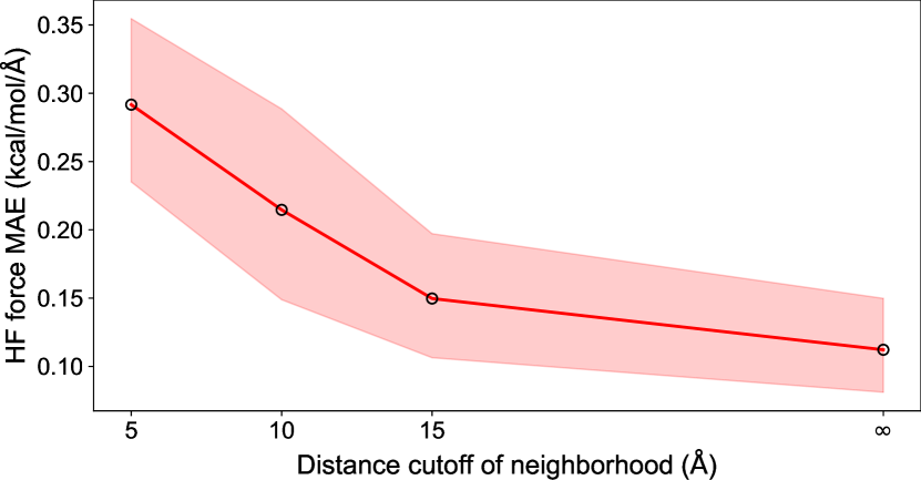
(b) HF force results

Figure 17: Ablation study results for the nonlocality of the functional model architecture. (a) and (b) show the energy error and HF force error of M-OFDFT on 50 QMugs molecules with 56-60 heavy atoms, for which the model is trained on QM9 and QMugs molecules of no more than 15 heavy atoms. The distance cutoff $\infty$ represents a fully-connected graph (nonlocal model). The experiment is conducted on the extrapolation setting in parallel with Supplementary Table 6.

D.4.3 Local Frame and Enhancement Modules

As discussed in Methods 4.2, the input coefficients are tensors equivariant to rotation, but the output energy is a scalar hence invariant, which requires the model to have such invariance built-in. In addition, the vast range of gradient data makes optimizing the KEDF model challenging. A CoefficientAdapter module is proposed to guarantee the geometric invariance of the model and express the vast gradient range. We conducted an ablation experiment to study the importance of each component in this module. As shown in Supplementary Table 8, utilizing the local frame results in a considerable performance improvement compared to the baseline model using the standard global frame (e.g., derived by PCA on the atom coordinates), demonstrating the effectiveness of the local frame in reducing the geometric variability of input data.

Furthermore, since different basis functions have varying importance in representing a density, some coefficient dimensions can significantly influence the density function and the electronic energy. This is difficult for M-OFDFT to handle, as the model treats each dimension equally. During density optimization, this influence is amplified when the input density is far from the ground state. We address this issue by introducing the natural reparameterization technique to balance the impact of each coefficient dimension. The results in Supplementary Table 8 show that implementing natural reparameterization can significantly improve the performance of the model, especially for the Hückel initialization, which is far from the ground-state density. Here, the energy MAE is reduced by one or two orders of magnitude, highlighting the powerful capability of natural reparameterization in balancing sensitivities across coefficient dimensions.

We also attempted to examine the importance of the other two enhancement modules, the atomic reference module and the dimension-wise rescaling module, but found it difficult to optimize the learning objective when removing either module from the model. Consequently, the unreasonable evaluation results are omitted in Supplementary Table 8. Moreover, the substantial impact on expressing a vast gradient range and the quantitative results for reducing geometric variability, as clarified in Supplementary Sec. B.3.1, also strongly support the necessity of these two modules.

Table 8: Ablation study for components in the CoefficientAdapter module. All results are evaluated on test ethanol molecules with the learned $T_{\textnormal{S,res},\theta}$ model. The MAEs in energy and HF force are listed in $\mathrm{kcal/mol}$ and $\mathrm{kcal/mol/\text{\r{A}}}$, respectively.

Local Frame	Nat. Reparam.	Density Initialization	Energy	HF Force
		Hückel	567.69	73.17
		ProjMINAO	0.57	2.02
✓		Hückel	514.56	36.55
		ProjMINAO	0.30	1.29
	✓	Hückel	25.41	37.18
		ProjMINAO	0.18	1.81
✓	✓	Hückel	5.77	27.73
		ProjMINAO	0.18	1.18

D.4.4 Results Using Other Training Strategies

As stressed in the main paper, one of the additional challenges for learning a functional model beyond conventional machine learning tasks is that the model is used to construct an objective function for optimizing the input, hence in addition to accurate end-to-end prediction on a discrete set of input queries, the model also needs to capture the output landscape (tendency of change in each locality) to properly guide the optimization. To address this challenge, we introduced techniques to generate multiple density data points each also with a gradient label for each molecular structure (Methods 4.1, Supplementary Sec. A.4), which provides a more holistic depiction of the output landscape. While there are alternative methods to regularize the optimization behavior in the context of learning the XC functional model [55, 54, 56, 53], our experiments indicate that they are not as effective for our task.

Kirkpatrick et al. [55] design an SCF loss based on second-order perturbation theory to regularize the functional stationary at provided self-consistent solutions. This effectively acts as a gradient supervision at the ground state, i.e., the given self-consistent orbitals, for each molecular structure. The SCF loss itself is not directly suitable for learning the KEDF model as it is for supervising the gradient w.r.t orbitals but not density (also explained by del Mazo-Sevillano and Hermann [28]). Approaches under the same spirit to supervise the gradient at the electronic ground state of each molecular structure are also explored in learning a KEDF model [29, 30, 32, 28]. In contrast, M-OFDFT introduces gradient labels on multiple electronic density states, instead of only the ground-state density, for each molecular structure, which provides richer and broader landscape information, leading to a substantial performance improvement as shown in our ablation study results in Supplementary Table 7 (row 1 and row 3).

Other studies shape the output landscape and regularize the optimization behavior by directly supervising the model-optimized energy and density (or orbitals). This approach supervises the end goal, but unfortunately complicates the learning process of the model, since the dependency of the model-optimized results on model parameters is nested iteratively following an optimization iteration. Some works resort to gradient-free optimization methods (e.g., evolutionary-style algorithms) to optimize the model parameters [54], which are inefficient. Li et al. [56] choose to directly invoke automatic differentiation on the loss w.r.t model parameters through the optimization process of orbitals, which is, in the context of learning the XC functional for KSDFT, typically conducted through the self-consistency field (SCF) iteration that solves the Kohn-Sham equations, hence called the Kohn-Sham regularizer. We tried its counterpart for learning the KEDF for OFDFT, by supervising the model-optimized energy and density after the density optimization process using gradient descent (note SCF iteration is unnatural here), and then applying automatic differentiation through the gradient-descent iteration. In our experiments on QM9, we found this incurs significant more computational cost for computing the gradient for model parameters. Even only using the $E_{\textnormal{TXC}}$ version of functional model (Supplementary Sec. B.4.2) to get rid of the costly grid-based computation, only a few number of density optimization steps up to 8 is affordable. With this maximally affordable cost, this strategy could work when applied to an end-to-end pretrained model on the energy and gradient labels, as we observed improved energy accuracy on held-out test molecules using 8 steps of density optimization. However, an undesired observation indicates that the model learned in this way still does not meet the goal: the density optimization process often does not converge, and even when it does, the accuracy is much worse than that at the 8-th step. This makes the method, instead of learning a density functional that holds a physical meaning, more like an end-to-end ground-state energy predictor constructed by unrolling the machine-learning model 8 times through the gradient descent process.

Under the same idea to supervise model-optimized energy, Chen et al. [53] find it is possible to avoid automatic differentiation through the iterative orbital optimization process if the resulting energy $E_{\theta}(\mathbf{C}_{\theta}^{\star})$ is indeed optimal in the view of the current functional model, since $\nabla_{\theta}E_{\theta}(\mathbf{C}_{\theta}^{\star})=(\nabla_{\theta}E_{\theta})\big{|}_{\mathbf{C}_{\theta}^{\star}}+(\nabla_{\theta}{\bar{\mathbf{C}}}_{\theta}^{\star})^{\top}(\nabla_{\bar{\mathbf{C}}}E_{\theta})\big{|}_{{\bar{\mathbf{C}}}_{\theta}^{\star}}=(\nabla_{\theta}E_{\theta})\big{|}_{\mathbf{C}_{\theta}^{\star}}$ ($\bar{\mathbf{C}}$ denotes the vector of flattened $\mathbf{C}$ matrix, and $\nabla_{\theta}{\bar{\mathbf{C}}}_{\theta}^{\star}$ is the Jacobian matrix) as the optimality condition indicates $(\nabla_{\bar{\mathbf{C}}}E_{\theta})\big{|}_{{\bar{\mathbf{C}}}_{\theta}^{\star}}=0$ on the admissible space of orbital coefficients, so $\nabla_{\theta}{\bar{\mathbf{C}}}_{\theta}^{\star}$ is avoided. The same argument also applies to the optimization process of density coefficients. Since finding the optimal orbitals after every model update is expensive, the method opts to optimize the model and density alternately. However, this modification biases the orbital/density optimality thus the optimization process may also deviate from being effective. In our experiment on Chignolin, we iterated the alternate optimization for four steps (and even carefully optimized the density in each step with a large cost), but observed only marginal performance improvement. Specifically, the performance gains from each step are 0.5%, -0.06%, 1.7%, and -0.8%, respectively, where the negative signs indicate that some steps even worsen the results.

References

- Seminario [1996] Jorge M Seminario. Recent developments and applications of modern density functional theory. 1996.
- Jain et al. [2013] Anubhav Jain, Shyue Ping Ong, Geoffroy Hautier, Wei Chen, William Davidson Richards, Stephen Dacek, Shreyas Cholia, Dan Gunter, David Skinner, Gerbrand Ceder, and Kristin A. Persson. Commentary: The Materials Project: A materials genome approach to accelerating materials innovation. APL Materials, 1(1):011002, 07 2013. ISSN 2166-532X. doi: 10.1063/1.4812323. URL https://doi.org/10.1063/1.4812323.
- Kohn and Sham [1965] Walter Kohn and Lu Jeu Sham. Self-consistent equations including exchange and correlation effects. Physical review, 140(4A):A1133, 1965.
- Thomas [1927] Llewellyn H Thomas. The calculation of atomic fields. In Mathematical proceedings of the Cambridge philosophical society, volume 23, pages 542–548. Cambridge University Press, 1927.
- Fermi [1928] Enrico Fermi. Eine statistische methode zur bestimmung einiger eigenschaften des atoms und ihre anwendung auf die theorie des periodischen systems der elemente. Zeitschrift für Physik, 48(1):73–79, 1928.
- Slater [1951] John C Slater. A simplification of the Hartree-Fock method. Physical review, 81(3):385, 1951.
- Hohenberg and Kohn [1964] Pierre Hohenberg and Walter Kohn. Inhomogeneous electron gas. Physical review, 136(3B):B864, 1964.
- Wang and Carter [2000] Yan Alexander Wang and Emily A Carter. Orbital-free kinetic-energy density functional theory. Theoretical methods in condensed phase chemistry, 5:117–84, 2000.
- Karasiev et al. [2014] Valentin V Karasiev, Debajit Chakraborty, and SB Trickey. Progress on new approaches to old ideas: Orbital-free density functionals. In Many-electron approaches in physics, chemistry and mathematics: a multidisciplinary view, pages 113–134. Springer, 2014.
- Witt et al. [2018] William C Witt, G Beatriz, Johannes M Dieterich, and Emily A Carter. Orbital-free density functional theory for materials research. Journal of Materials Research, 33(7):777–795, 2018.
- Hodges [1973] C. H. Hodges. Quantum corrections to the Thomas–Fermi approximation — the Kirzhnits method. Canadian Journal of Physics, 51(13):1428–1437, 1973. doi: 10.1139/p73-189. URL https://doi.org/10.1139/p73-189.
- Brack et al. [1976] M. Brack, B.K. Jennings, and Y.H. Chu. On the extended Thomas-Fermi approximation to the kinetic energy density. Physics Letters B, 65(1):1–4, 1976. ISSN 0370-2693. doi: https://doi.org/10.1016/0370-2693(76)90519-0. URL https://www.sciencedirect.com/science/article/pii/0370269376905190.
- Wang and Teter [1992] Lin-Wang Wang and Michael P Teter. Kinetic-energy functional of the electron density. Physical Review B, 45(23):13196, 1992.
- Wang et al. [1999] Yan Alexander Wang, Niranjan Govind, and Emily A Carter. Orbital-free kinetic-energy density functionals with a density-dependent kernel. Physical Review B, 60(24):16350, 1999.
- Huang and Carter [2010] Chen Huang and Emily A Carter. Nonlocal orbital-free kinetic energy density functional for semiconductors. Physical Review B, 81(4):045206, 2010.
- Zhou et al. [2005] Baojing Zhou, Vincent L Ligneres, and Emily A Carter. Improving the orbital-free density functional theory description of covalent materials. The Journal of chemical physics, 122(4), 2005.
- Qiu et al. [2017] Ruizhi Qiu, Haiyan Lu, Bingyun Ao, Li Huang, Tao Tang, and Piheng Chen. Energetics of intrinsic point defects in aluminium via orbital-free density functional theory. Philosophical Magazine, 97(25):2164–2181, 2017.
- García-Aldea and Alvarellos [2007] David García-Aldea and JE Alvarellos. Kinetic energy density study of some representative semilocal kinetic energy functionals. The Journal of chemical physics, 127(14), 2007.
- Xia et al. [2012] Junchao Xia, Chen Huang, Ilgyou Shin, and Emily A Carter. Can orbital-free density functional theory simulate molecules? The Journal of chemical physics, 136(8):084102, 2012.
- Sillaste and Thompson [2022] Spencer Sillaste and Russell B Thompson. Molecular bonding in an orbital-free-related density functional theory. The Journal of Physical Chemistry A, 126(2):325–332, 2022.
- Teale et al. [2022] Andrew M Teale, Trygve Helgaker, Andreas Savin, Carlo Adamo, Bálint Aradi, Alexei V Arbuznikov, Paul W Ayers, Evert Jan Baerends, Vincenzo Barone, Patrizia Calaminici, et al. DFT exchange: sharing perspectives on the workhorse of quantum chemistry and materials science. Physical chemistry chemical physics, 24(47):28700–28781, 2022.
- García-González et al. [1996] P. García-González, J. E. Alvarellos, and E. Chacón. Nonlocal kinetic-energy-density functionals. Phys. Rev. B, 53:9509–9512, Apr 1996. doi: 10.1103/PhysRevB.53.9509. URL https://link.aps.org/doi/10.1103/PhysRevB.53.9509.
- Mi et al. [2018] Wenhui Mi, Alessandro Genova, and Michele Pavanello. Nonlocal kinetic energy functionals by functional integration. The Journal of Chemical Physics, 148(18):184107, 05 2018. ISSN 0021-9606. doi: 10.1063/1.5023926. URL https://doi.org/10.1063/1.5023926.
- Snyder et al. [2012] John C Snyder, Matthias Rupp, Katja Hansen, Klaus-Robert Müller, and Kieron Burke. Finding density functionals with machine learning. Physical review letters, 108(25):253002, 2012.
- Snyder et al. [2013] John C Snyder, Matthias Rupp, Katja Hansen, Leo Blooston, Klaus-Robert Müller, and Kieron Burke. Orbital-free bond breaking via machine learning. The Journal of chemical physics, 139(22):224104, 2013.
- Li et al. [2016] Li Li, Thomas E Baker, Steven R White, Kieron Burke, et al. Pure density functional for strong correlation and the thermodynamic limit from machine learning. Physical Review B, 94(24):245129, 2016.
- Brockherde et al. [2017] Felix Brockherde, Leslie Vogt, Li Li, Mark E Tuckerman, Kieron Burke, and Klaus-Robert Müller. Bypassing the Kohn-Sham equations with machine learning. Nature communications, 8(1):1–10, 2017.
- del Mazo-Sevillano and Hermann [2023] Pablo del Mazo-Sevillano and Jan Hermann. Variational principle to regularize machine-learned density functionals: the non-interacting kinetic-energy functional. arXiv preprint arXiv:2306.17587, 2023.
- Meyer et al. [2020] Ralf Meyer, Manuel Weichselbaum, and Andreas W Hauser. Machine learning approaches toward orbital-free density functional theory: Simultaneous training on the kinetic energy density functional and its functional derivative. Journal of chemical theory and computation, 16(9):5685–5694, 2020.
- Fujinami et al. [2020] Mikito Fujinami, Ryo Kageyama, Junji Seino, Yasuhiro Ikabata, and Hiromi Nakai. Orbital-free density functional theory calculation applying semi-local machine-learned kinetic energy density functional and kinetic potential. Chemical Physics Letters, 748:137358, 2020.
- Ryczko et al. [2021] Kevin Ryczko, Sebastian J Wetzel, Roger G Melko, and Isaac Tamblyn. Orbital-free density functional theory with small datasets and deep learning. arXiv preprint arXiv:2104.05408, 2021.
- Imoto et al. [2021] Fumihiro Imoto, Masatoshi Imada, and Atsushi Oshiyama. Order-N orbital-free density-functional calculations with machine learning of functional derivatives for semiconductors and metals. Physical Review Research, 3(3):033198, 2021.
- Ying et al. [2021] Chengxuan Ying, Tianle Cai, Shengjie Luo, Shuxin Zheng, Guolin Ke, Di He, Yanming Shen, and Tie-Yan Liu. Do Transformers really perform badly for graph representation? Advances in Neural Information Processing Systems, 34:28877–28888, 2021.
- Shi et al. [2022] Yu Shi, Shuxin Zheng, Guolin Ke, Yifei Shen, Jiacheng You, Jiyan He, Shengjie Luo, Chang Liu, Di He, and Tie-Yan Liu. Benchmarking Graphormer on large-scale molecular modeling datasets. arXiv preprint arXiv:2203.04810, 2022.
- Vaswani et al. [2017] Ashish Vaswani, Noam Shazeer, Niki Parmar, Jakob Uszkoreit, Llion Jones, Aidan N Gomez, Łukasz Kaiser, and Illia Polosukhin. Attention is all you need. Advances in neural information processing systems, 30, 2017.
- Kato [1957] Tosio Kato. On the eigenfunctions of many-particle systems in quantum mechanics. Communications on Pure and Applied Mathematics, 10(2):151–177, 1957.
- Chmiela et al. [2017] Stefan Chmiela, Alexandre Tkatchenko, Huziel E Sauceda, Igor Poltavsky, Kristof T Schütt, and Klaus-Robert Müller. Machine learning of accurate energy-conserving molecular force fields. Science advances, 3(5):e1603015, 2017.
- Chmiela et al. [2019] Stefan Chmiela, Huziel E Sauceda, Igor Poltavsky, Klaus-Robert Müller, and Alexandre Tkatchenko. sGDML: Constructing accurate and data efficient molecular force fields using machine learning. Computer Physics Communications, 240:38–45, 2019.
- Ruddigkeit et al. [2012] Lars Ruddigkeit, Ruud Van Deursen, Lorenz C Blum, and Jean-Louis Reymond. Enumeration of 166 billion organic small molecules in the chemical universe database GDB-17. Journal of chemical information and modeling, 52(11):2864–2875, 2012.
- Ramakrishnan et al. [2014] Raghunathan Ramakrishnan, Pavlo O Dral, Matthias Rupp, and O Anatole von Lilienfeld. Quantum chemistry structures and properties of 134 kilo molecules. Scientific Data, 1, 2014.
- Constantin et al. [2011] Lucian A Constantin, E Fabiano, S Laricchia, and F Della Sala. Semiclassical neutral atom as a reference system in density functional theory. Physical review letters, 106(18):186406, 2011.
- Karasiev and Trickey [2012] Valentin V Karasiev and Samuel B Trickey. Issues and challenges in orbital-free density functional calculations. Computer Physics Communications, 183(12):2519–2527, 2012.
- Weizsäcker [1935] CF von Weizsäcker. Zur theorie der kernmassen. Zeitschrift für Physik, 96(7):431–458, 1935.
- Smith et al. [2017] Justin S Smith, Olexandr Isayev, and Adrian E Roitberg. ANI-1: an extensible neural network potential with DFT accuracy at force field computational cost. Chemical science, 8(4):3192–3203, 2017.
- Isert et al. [2022] Clemens Isert, Kenneth Atz, José Jiménez-Luna, and Gisbert Schneider. QMugs, quantum mechanical properties of drug-like molecules. Scientific Data, 9(1):1–11, 2022.
- Du and Mordatch [2019] Yilun Du and Igor Mordatch. Implicit generation and generalization in energy-based models. arXiv preprint arXiv:1903.08689, 2019.
- Du et al. [2022] Yilun Du, Shuang Li, Joshua Tenenbaum, and Igor Mordatch. Learning iterative reasoning through energy minimization. In International Conference on Machine Learning, pages 5570–5582. PMLR, 2022.
- Lindorff-Larsen et al. [2011] Kresten Lindorff-Larsen, Stefano Piana, Ron O Dror, and David E Shaw. How fast-folding proteins fold. Science, 334(6055):517–520, 2011.
- Neuweiler et al. [2009] Hannes Neuweiler, Timothy D Sharpe, Trevor J Rutherford, Christopher M Johnson, Mark D Allen, Neil Ferguson, and Alan R Fersht. The folding mechanism of BBL: Plasticity of transition-state structure observed within an ultrafast folding protein family. Journal of molecular biology, 390(5):1060–1073, 2009.
- Wang et al. [2004] Ting Wang, Yongjin Zhu, and Feng Gai. Folding of a three-helix bundle at the folding speed limit. The Journal of Physical Chemistry B, 108(12):3694–3697, 2004.
- Rayson and Briddon [2008] Mark J Rayson and Patrick R Briddon. Rapid iterative method for electronic-structure eigenproblems using localised basis functions. Computer Physics Communications, 178(2):128–134, 2008.
- Dick and Fernandez-Serra [2020] Sebastian Dick and Marivi Fernandez-Serra. Machine learning accurate exchange and correlation functionals of the electronic density. Nature communications, 11(1):3509, 2020.
- Chen et al. [2021] Yixiao Chen, Linfeng Zhang, Han Wang, and Weinan E. DeePKS: A comprehensive data-driven approach toward chemically accurate density functional theory. Journal of Chemical Theory and Computation, 17(1):170–181, 2021.
- Nagai et al. [2020] Ryo Nagai, Ryosuke Akashi, and Osamu Sugino. Completing density functional theory by machine learning hidden messages from molecules. npj Computational Materials, 6(1):1–8, 2020.
- Kirkpatrick et al. [2021] James Kirkpatrick, Brendan McMorrow, David HP Turban, Alexander L Gaunt, James S Spencer, Alexander GDG Matthews, Annette Obika, Louis Thiry, Meire Fortunato, David Pfau, et al. Pushing the frontiers of density functionals by solving the fractional electron problem. Science, 374(6573):1385–1389, 2021.
- Li et al. [2021a] Li Li, Stephan Hoyer, Ryan Pederson, Ruoxi Sun, Ekin D Cubuk, Patrick Riley, Kieron Burke, et al. Kohn-Sham equations as regularizer: Building prior knowledge into machine-learned physics. Physical review letters, 126(3):036401, 2021a.
- Kawaguchi et al. [2022] K. Kawaguchi, Y. Bengio, and L. Kaelbling. Generalization in Deep Learning, page 112–148. Cambridge University Press, 2022. doi: 10.1017/9781009025096.003.
- Huang et al. [2023] Bing Huang, Guido Falk von Rudorff, and O Anatole von Lilienfeld. The central role of density functional theory in the AI age. Science, 381(6654):170–175, 2023.
- Zhang et al. [2023] Xuan Zhang, Limei Wang, Jacob Helwig, Youzhi Luo, Cong Fu, Yaochen Xie, Meng Liu, Yuchao Lin, Zhao Xu, Keqiang Yan, et al. Artificial intelligence for science in quantum, atomistic, and continuum systems. arXiv preprint arXiv:2307.08423, 2023.
- Lieb [1983] Elliott H Lieb. Density functionals for Coulomb systems. International Journal of Quantum Chemistry, 24(3):243–277, 1983.
- Brown et al. [2020] Tom Brown, Benjamin Mann, Nick Ryder, Melanie Subbiah, Jared D Kaplan, Prafulla Dhariwal, Arvind Neelakantan, Pranav Shyam, Girish Sastry, Amanda Askell, et al. Language models are few-shot learners. Advances in neural information processing systems, 33:1877–1901, 2020.
- Zhao et al. [2023] Wayne Xin Zhao, Kun Zhou, Junyi Li, Tianyi Tang, Xiaolei Wang, Yupeng Hou, Yingqian Min, Beichen Zhang, Junjie Zhang, Zican Dong, et al. A survey of large language models. arXiv preprint arXiv:2303.18223, 2023.
- Zheng et al. [2023] Shuxin Zheng, Jiyan He, Chang Liu, Yu Shi, Ziheng Lu, Weitao Feng, Fusong Ju, Jiaxi Wang, Jianwei Zhu, Yaosen Min, Zhang He, Shidi Tang, Hongxia Hao, Peiran Jin, Chi Chen, Frank Noé, Haiguang Liu, and Tie-Yan Liu. Towards predicting equilibrium distributions for molecular systems with deep learning. arXiv preprint arXiv:2306.05445, 2023.
- Dunlap [2000] Brett I. Dunlap. Robust and variational fitting. Phys. Chem. Chem. Phys., 2:2113–2116, 2000. doi: 10.1039/B000027M. URL http://dx.doi.org/10.1039/B000027M.
- Bardo and Ruedenberg [1974] Richard D. Bardo and Klaus Ruedenberg. Even-tempered atomic orbitals. VI. optimal orbital exponents and optimal contractions of Gaussian primitives for hydrogen, carbon, and oxygen in molecules. The Journal of Chemical Physics, 60(3):918–931, 1974. doi: 10.1063/1.1681168. URL https://doi.org/10.1063/1.1681168.
- Satorras et al. [2021] Vıctor Garcia Satorras, Emiel Hoogeboom, and Max Welling. E (n) equivariant graph neural networks. In International conference on machine learning, pages 9323–9332. PMLR, 2021.
- Thomas et al. [2018] Nathaniel Thomas, Tess Smidt, Steven Kearnes, Lusann Yang, Li Li, Kai Kohlhoff, and Patrick Riley. Tensor field networks: Rotation-and translation-equivariant neural networks for 3d point clouds. arXiv preprint arXiv:1802.08219, 2018.
- Han et al. [2018] Jiequn Han, Linfeng Zhang, Roberto Car, et al. Deep Potential: A general representation of a many-body potential energy surface. Communications in Computational Physics, 23(3), 2018.
- Li et al. [2022] He Li, Zun Wang, Nianlong Zou, Meng Ye, Runzhang Xu, Xiaoxun Gong, Wenhui Duan, and Yong Xu. Deep-learning density functional theory Hamiltonian for efficient ab initio electronic-structure calculation. Nature Computational Science, 2(6):367–377, 2022.
- Li et al. [2021b] Feiran Li, Kent Fujiwara, Fumio Okura, and Yasuyuki Matsushita. A closer look at rotation-invariant deep point cloud analysis. In Proceedings of the IEEE/CVF International Conference on Computer Vision, pages 16218–16227, 2021b.
- Puny et al. [2021] Omri Puny, Matan Atzmon, Heli Ben-Hamu, Ishan Misra, Aditya Grover, Edward J Smith, and Yaron Lipman. Frame averaging for invariant and equivariant network design. arXiv preprint arXiv:2110.03336, 2021.
- Fuchs et al. [2020] Fabian Fuchs, Daniel Worrall, Volker Fischer, and Max Welling. Se (3)-transformers: 3d roto-translation equivariant attention networks. Advances in neural information processing systems, 33:1970–1981, 2020.
- Schütt et al. [2021] Kristof Schütt, Oliver Unke, and Michael Gastegger. Equivariant message passing for the prediction of tensorial properties and molecular spectra. In International Conference on Machine Learning, pages 9377–9388. PMLR, 2021.
- Batzner et al. [2022] Simon Batzner, Albert Musaelian, Lixin Sun, Mario Geiger, Jonathan P Mailoa, Mordechai Kornbluth, Nicola Molinari, Tess E Smidt, and Boris Kozinsky. E (3)-equivariant graph neural networks for data-efficient and accurate interatomic potentials. Nature communications, 13(1):2453, 2022.
- Musaelian et al. [2023] Albert Musaelian, Simon Batzner, Anders Johansson, Lixin Sun, Cameron J Owen, Mordechai Kornbluth, and Boris Kozinsky. Learning local equivariant representations for large-scale atomistic dynamics. Nature Communications, 14(1):579, 2023.
- Fazlyab et al. [2019] Mahyar Fazlyab, Alexander Robey, Hamed Hassani, Manfred Morari, and George Pappas. Efficient and accurate estimation of lipschitz constants for deep neural networks. Advances in Neural Information Processing Systems, 32, 2019.
- Amari [1998] Shun-Ichi Amari. Natural gradient works efficiently in learning. Neural computation, 10(2):251–276, 1998.
- Yoshikawa and Sumita [2022] Naruki Yoshikawa and Masato Sumita. Automatic differentiation for the direct minimization approach to the Hartree–Fock method. The Journal of Physical Chemistry A, 126(45):8487–8493, 2022.
- Sun et al. [2018] Qiming Sun, Timothy C Berkelbach, Nick S Blunt, George H Booth, Sheng Guo, Zhendong Li, Junzi Liu, James D McClain, Elvira R Sayfutyarova, Sandeep Sharma, et al. PySCF: the Python-based simulations of chemistry framework. Wiley Interdisciplinary Reviews: Computational Molecular Science, 8(1):e1340, 2018.
- Hoffmann [1963] Roald Hoffmann. An Extended Hückel Theory. I. Hydrocarbons. The Journal of Chemical Physics, 39(6):1397–1412, 06 1963. ISSN 0021-9606. doi: 10.1063/1.1734456. URL https://doi.org/10.1063/1.1734456.
- Lehtola [2019] Susi Lehtola. Assessment of initial guesses for self-consistent field calculations. Superposition of atomic potentials: Simple yet efficient. Journal of chemical theory and computation, 15(3):1593–1604, 2019.
- Levy [1979] Mel Levy. Universal variational functionals of electron densities, first-order density matrices, and natural spin-orbitals and solution of the v-representability problem. Proceedings of the National Academy of Sciences, 76(12):6062–6065, 1979.
- Bobrowicz and Goddard [1977] Frank W. Bobrowicz and William A. Goddard. The Self-Consistent Field Equations for Generalized Valence Bond and Open-Shell Hartree-Fock Wave Functions, pages 79–127. Springer US, Boston, MA, 1977. ISBN 978-1-4757-0887-5. doi: 10.1007/978-1-4757-0887-5˙4. URL https://doi.org/10.1007/978-1-4757-0887-5_4.
- Levine et al. [2009] Ira N Levine, Daryle H Busch, and Harrison Shull. Quantum chemistry, volume 6. Pearson Prentice Hall Upper Saddle River, NJ, 2009.
- Blinder [1965] SM Blinder. Basic concepts of self-consistent-field theory. American journal of physics, 33(6):431–443, 1965.
- Pulay [1982] P. Pulay. Improved scf convergence acceleration. Journal of Computational Chemistry, 3(4):556–560, 1982. doi: https://doi.org/10.1002/jcc.540030413. URL https://onlinelibrary.wiley.com/doi/abs/10.1002/jcc.540030413.
- Kudin et al. [2002] Konstantin N. Kudin, Gustavo E. Scuseria, and Eric Cancès. A black-box self-consistent field convergence algorithm: One step closer. The Journal of Chemical Physics, 116(19):8255–8261, 04 2002. ISSN 0021-9606. doi: 10.1063/1.1470195. URL https://doi.org/10.1063/1.1470195.
- Dupuis et al. [1976] Michel Dupuis, John Rys, and Harry F. King. Evaluation of molecular integrals over Gaussian basis functions. The Journal of Chemical Physics, 65(1):111–116, 07 1976. ISSN 0021-9606. doi: 10.1063/1.432807. URL https://doi.org/10.1063/1.432807.
- Rys et al. [1983] J. Rys, M. Dupuis, and H. F. King. Computation of electron repulsion integrals using the rys quadrature method. Journal of Computational Chemistry, 4(2):154–157, 1983. doi: https://doi.org/10.1002/jcc.540040206. URL https://onlinelibrary.wiley.com/doi/abs/10.1002/jcc.540040206.
- Sun [2015] Qiming Sun. Libcint: An efficient general integral library for Gaussian basis functions. Journal of computational chemistry, 36(22):1664–1671, 2015.
- Baydin et al. [2018] Atilim Gunes Baydin, Barak A Pearlmutter, Alexey Andreyevich Radul, and Jeffrey Mark Siskind. Automatic differentiation in machine learning: a survey. Journal of Marchine Learning Research, 18:1–43, 2018.
- Paszke et al. [2019] Adam Paszke, Sam Gross, Francisco Massa, Adam Lerer, James Bradbury, Gregory Chanan, Trevor Killeen, Zeming Lin, Natalia Gimelshein, Luca Antiga, et al. Pytorch: An imperative style, high-performance deep learning library. Advances in neural information processing systems, 32, 2019.
- Perdew et al. [1996] John P Perdew, Kieron Burke, and Matthias Ernzerhof. Generalized gradient approximation made simple. Physical review letters, 77(18):3865, 1996.
- Parr and Yang [1989] Robert G Parr and Weitao Yang. Density-functional theory of atoms and molecules. 1989.
- Hollingsworth et al. [2018] Jacob Hollingsworth, Li Li, Thomas E Baker, and Kieron Burke. Can exact conditions improve machine-learned density functionals? The Journal of chemical physics, 148(24):241743, 2018.
- Kalita et al. [2021] Bhupalee Kalita, Li Li, Ryan J McCarty, and Kieron Burke. Learning to approximate density functionals. Accounts of Chemical Research, 54(4):818–826, 2021.
- Changyong et al. [2014] Feng Changyong, Wang Hongyue, Lu Naiji, Chen Tian, He Hua, Lu Ying, et al. Log-transformation and its implications for data analysis. Shanghai archives of psychiatry, 26(2):105, 2014.
- Wang et al. [2019] Jiang Wang, Simon Olsson, Christoph Wehmeyer, Adrià Pérez, Nicholas E Charron, Gianni De Fabritiis, Frank Noé, and Cecilia Clementi. Machine learning of coarse-grained molecular dynamics force fields. ACS central science, 5(5):755–767, 2019.
- Pérez-Hernández et al. [2013] Guillermo Pérez-Hernández, Fabian Paul, Toni Giorgino, Gianni De Fabritiis, and Frank Noé. Identification of slow molecular order parameters for markov model construction. The Journal of chemical physics, 139(1):07B604_1, 2013.
- Schwantes and Pande [2013] Christian R Schwantes and Vijay S Pande. Improvements in markov state model construction reveal many non-native interactions in the folding of NTL9. Journal of chemical theory and computation, 9(4):2000–2009, 2013.
- McGibbon et al. [2015] Robert T McGibbon, Kyle A Beauchamp, Matthew P Harrigan, Christoph Klein, Jason M Swails, Carlos X Hernández, Christian R Schwantes, Lee-Ping Wang, Thomas J Lane, and Vijay S Pande. Mdtraj: a modern open library for the analysis of molecular dynamics trajectories. Biophysical journal, 109(8):1528–1532, 2015.
- Eastman et al. [2017] Peter Eastman, Jason Swails, John D Chodera, Robert T McGibbon, Yutong Zhao, Kyle A Beauchamp, Lee-Ping Wang, Andrew C Simmonett, Matthew P Harrigan, Chaya D Stern, et al. OpenMM 7: Rapid development of high performance algorithms for molecular dynamics. PLoS computational biology, 13(7):e1005659, 2017.
- Case et al. [2008] David A Case, Tom A Darden, Thomas E Cheatham, Carlos L Simmerling, Junmei Wang, Robert E Duke, Ray Luo, MRCW Crowley, Ross C Walker, Wei Zhang, et al. Amber 10. Technical report, University of California, 2008.
- Becke [1993] Axel D. Becke. Density-functional thermochemistry. III. The role of exact exchange. The Journal of Chemical Physics, 98, 1993. ISSN 00219606. doi: 10.1063/1.464913.
- Stephens et al. [1994] Philip J Stephens, Frank J Devlin, Cary F Chabalowski, and Michael J Frisch. Ab initio calculation of vibrational absorption and circular dichroism spectra using density functional force fields. The Journal of physical chemistry, 98(45):11623–11627, 1994.
- Weigend [2006] Florian Weigend. Accurate coulomb-fitting basis sets for h to rn. Phys. Chem. Chem. Phys., 8:1057, 2006. doi: 10.1039/b515623h.
- Ho et al. [2008] Gregory S Ho, Vincent L Lignères, and Emily A Carter. Introducing PROFESS: A new program for orbital-free density functional theory calculations. Computer physics communications, 179(11):839–854, 2008.
- Enkovaara et al. [2010] Jussi Enkovaara, Carsten Rostgaard, J Jørgen Mortensen, Jingzhe Chen, M Dułak, Lara Ferrighi, Jeppe Gavnholt, Christian Glinsvad, V Haikola, HA Hansen, et al. Electronic structure calculations with GPAW: a real-space implementation of the projector augmented-wave method. Journal of physics: Condensed matter, 22(25):253202, 2010.
- Mi et al. [2016] Wenhui Mi, Xuecheng Shao, Chuanxun Su, Yuanyuan Zhou, Shoutao Zhang, Quan Li, Hui Wang, Lijun Zhang, Maosheng Miao, Yanchao Wang, et al. ATLAS: A real-space finite-difference implementation of orbital-free density functional theory. Computer Physics Communications, 200:87–95, 2016.
- Shao et al. [2021] Xuecheng Shao, Kaili Jiang, Wenhui Mi, Alessandro Genova, and Michele Pavanello. DFTpy: An efficient and object-oriented platform for orbital-free dft simulations. Wiley Interdisciplinary Reviews: Computational Molecular Science, 11(1):e1482, 2021.
- Hellman [1937] Hans Hellman. Einführung in die Quantenchemie. Franz Deuticke, Leipzig, 285, 1937.
- Feynman [1939] R. P. Feynman. Forces in molecules. Phys. Rev., 56:340–343, Aug 1939. doi: 10.1103/PhysRev.56.340. URL https://link.aps.org/doi/10.1103/PhysRev.56.340.
- Pulay [1969] Peter Pulay. Ab initio calculation of force constants and equilibrium geometries in polyatomic molecules: I. Theory. Molecular Physics, 17(2):197–204, 1969.
- Schütt et al. [2018] Kristof T Schütt, Huziel E Sauceda, P-J Kindermans, Alexandre Tkatchenko, and K-R Müller. Schnet–a deep learning architecture for molecules and materials. The Journal of Chemical Physics, 148(24), 2018.
- Branch et al. [1999] Mary Ann Branch, Thomas F Coleman, and Yuying Li. A subspace, interior, and conjugate gradient method for large-scale bound-constrained minimization problems. SIAM Journal on Scientific Computing, 21(1):1–23, 1999.
- Virtanen et al. [2020] Pauli Virtanen, Ralf Gommers, Travis E. Oliphant, Matt Haberland, Tyler Reddy, David Cournapeau, Evgeni Burovski, Pearu Peterson, Warren Weckesser, Jonathan Bright, Stéfan J. van der Walt, Matthew Brett, Joshua Wilson, K. Jarrod Millman, Nikolay Mayorov, Andrew R. J. Nelson, Eric Jones, Robert Kern, Eric Larson, C J Carey, İlhan Polat, Yu Feng, Eric W. Moore, Jake VanderPlas, Denis Laxalde, Josef Perktold, Robert Cimrman, Ian Henriksen, E. A. Quintero, Charles R. Harris, Anne M. Archibald, Antônio H. Ribeiro, Fabian Pedregosa, Paul van Mulbregt, and SciPy 1.0 Contributors. SciPy 1.0: Fundamental Algorithms for Scientific Computing in Python. Nature Methods, 17:261–272, 2020. doi: 10.1038/s41592-019-0686-2.