CRIMED: Lower and Upper Bounds on Regret
for Bandits with Unbounded Stochastic Corruption

Abstract

We investigate the regret-minimisation problem in a multi-armed bandit setting with arbitrary corruptions. Similar to the classical setup, the agent receives rewards generated independently from the distribution of the arm chosen at each time. However, these rewards are not directly observed. Instead, with a fixed $\varepsilon\in(0,\frac{1}{2})$, the agent observes a sample from the chosen arm’s distribution with probability $1-\varepsilon$, or from an arbitrary corruption distribution with probability $\varepsilon$. Importantly, we impose no assumptions on these corruption distributions, which can be unbounded. In this setting, accommodating potentially unbounded corruptions, we establish a problem-dependent lower bound on regret for a given family of arm distributions. We introduce CRIMED, an asymptotically-optimal algorithm that achieves the exact lower bound on regret for bandits with Gaussian distributions with known variance. Additionally, we provide a finite-sample analysis of CRIMED’s regret performance. Notably, CRIMED can effectively handle corruptions with $\varepsilon$ values as high as $\frac{1}{2}$. Furthermore, we develop a tight concentration result for medians in the presence of arbitrary corruptions, even with $\varepsilon$ values up to $\frac{1}{2}$, which may be of independent interest. We also discuss an extension of the algorithm for handling misspecification in Gaussian model.

1 Introduction

Multi-armed bandits are a widely-used statistical model in which an agent (or algorithm) interacts with the environment by selecting actions based on past observations and receives a reward for each chosen action. A classical objective is to minimise the regret, which is defined as the difference between the rewards accumulated by the algorithm and the rewards that would have been obtained by choosing the best action in hindsight at each step. In this paper, we delve into the problem of sequential decision-making under partial information, where the observations resulting from actions are susceptible to arbitrary yet stochastic corruption. More specifically, we explore a variant of the stochastic multi-armed bandit problem with unbounded stochastic corruption.

The algorithm is presented with a set of $K$ arms, each representing an unknown probability distribution from a given family of distributions $\mathcal{L}$. We denote this set of $K$-arms by $\mu\coloneqq(\mu_{1},\dots,\mu_{K})$, where $\forall a\in[K],\mu_{a}\in\mathcal{L}$. When the algorithm selects an arm $A_{n}$ at time $n$, an independent sample, $Y_{n}$, is drawn from the corresponding distribution $\mu_{A_{n}}$. This is the reward of the algorithm for pulling the chosen arm. However, unlike in the classical setup, $Y_{n}$ is not directly observed by the algorithm. Instead, the observations are subject to corruption with a known probability $\varepsilon\in(0,0.5)$: at time $n$, the algorithm observes $Y_{n}\sim\mu_{A_{n}}$ with probability $1-\varepsilon$, and with probability $\varepsilon$, it observes a sample from an arbitrary distribution $H_{A_{n},n}$. Let ${\bf H}_{n}\coloneqq(H_{1,n},\dots,H_{K,n})$ be the set of corruption distributions at time $n$. We place absolutely no assumptions on $H_{\cdot,n}$. Following the classical regret-minimisation setting, the goal of the algorithm in this partial-information setting is to sequentially sample these arms in order to maximize the expected cumulative reward when the observations are corrupted.

The bandit problem forms the theoretical cornerstone of modern Reinforcement Learning (RL) and serves as the algorithmic foundation for recommender systems. As both bandit problems and RL are increasingly finding practical applications, the question of robustness against corrupted or externally perturbed observations has gained considerable significance. This is particularly relevant because, in real-life applications such as finance, medicine, advertising, or recommender systems, algorithms often need to contend with corrupted data, as observations collected from multiple sources are susceptible to measurement or recording errors and inaccuracies.

In finance, the observed payoff data frequently contains outliers due to data contamination (Adams et al., 2019). In clinical research trials for new drugs and medical devices, outlier data can lead to false positive interventions and conclusions (Thabane et al., 2013). In online platforms and recommender systems, the ranking of products can get skewed by the appearance of small number of fake users (Golrezaei et al., 2021). The classical corruption-oblivious bandit algorithms, however, cannot effectively decide the arms to pull, when a possibly small fraction of the data may be subject to measurement errors or corruption. Specifically, a recent line of works (Jun et al., 2018; Liu and Shroff, 2019; Xu et al., 2021; Azize and Basu, 2023) show that one can make a classical bandit algorithms to incur linear regret by contaminating only a small amount of observations (logarithmic on horizon or even lower). These findings motivate us to study the bandit setup in the presence of arbitrary corruption, and design algorithms robust to it.

Researchers have broadly studied three types of settings: adversarial bandits  (Auer et al., 1995, 2002b), stochastic bandits with bounded adversarial corruptions, in which an adversary shifts the rewards under constraint on the total shift budget  (Lykouris et al., 2018; Gupta et al., 2019; Zimmert and Seldin, 2019), and more recently, unbounded stochastic corruption (Altschuler et al., 2019; Mukherjee et al., 2021; Basu et al., 2022). To the best of our knowledge, there is no established generic lower bound on regret in the context of unbounded stochastic corruptions, unlike in the first two settings. Furthermore, there is no known algorithm capable of yielding an appropriate upper bound on regret while also maintaining robustness. This paper aims to fill these two gaps by investigating bandits with unbounded stochastic corruptions.

Regret.  For $\mu\in\mathcal{L}^{K}$, let $m^{*}(\mu)$ denote the mean of the optimal arm in $\mu$ (arm with the maximum mean), and let $m(\mu_{a})$ denote the mean of arm $a$. For an arm $a$, let $\Delta_{a}\coloneqq m^{*}(\mu)-m(\mu_{a})$ denote the instantaneous mean regret incurred by pulling it. Recall that $Y_{n}$ denotes the independent (uncorrupted) sample drawn from the distribution associated with arm $A_{n}$. Let $Y_{a,j}$ denote the $j^{th}$ independent sample drawn from arm $a$.

Since in our setup, the observations are corrupted (while the rewards are uncorrupted), we define the expected regret under corruption till time $T$ as $\mathbb{E}\left[{R_{T}}\right]\coloneqq\mathbb{E}[{\sum\nolimits_{n=1}^{T}\left({m^{*}(\mu)-Y_{n}}\right)}]$. Here, the expectation is with respect to all the randomness present in the system, including the impact of corruption on action selection. See also (Kapoor et al., 2019; Basu et al., 2022) for a similar notion of regret. We further observe that $\mathbb{E}\left[{R_{T}}\right]=\sum\nolimits_{a=1}^{K}\mathbb{E}\left[{N_{a}(T)}\right]\Delta_{a},$ where $N_{a}(T)$ is the number of pulls of the arm $a$ till time $T$. Since $\Delta_{a}$’s are constant for a given $\mu$ and for the optimal arm(s) $\Delta_{a}=0$, minimising the expected regret reduces to minimise the expected number of pulls of the suboptimal arms $\mathbb{E}\left[{N_{a}(T)}\right]$.

Notation.  Let $\mathbb{R}$ and $\mathbb{R}^{+}$ denote the set of real numbers and non-negative real numbers, respectively, and let $\mathcal{P}(\mathbb{R})$ denote the set of all probability distributions on $\mathbb{R}$. For any set $S$, we denote by $2^{S}$ the set of subsets of $S$. For $\mu$, $n\in\mathbb{N}$, and ${\bf H}_{n}\in\mathcal{P}(\mathbb{R})^{K}$, let $\mu\odot_{\varepsilon}{\bf H}_{n}\coloneqq(1-\varepsilon)\mu+\varepsilon{\bf H}_{n}$ denote the vector of distributions in $\mu$ corrupted by corruption distributions in ${\bf H}_{n}$ with corruption proportion $\varepsilon$. We use a similar notation for each component $\mu_{a},H_{a,n}\in\mathcal{P}(\mathbb{R})$, i.e. $\mu_{a}\odot_{\varepsilon}H_{a,n}\coloneqq(1-\varepsilon)\mu_{a}+\varepsilon H_{a,n}$ for $a\in[K]$. Additionally, by $\bf H_{T}$, we denote the $T\times K$ matrix of corruption distributions with $\left\{{{\bf H}_{n}:n\in[T]}\right\}$ as rows. Finally, we denote by $\mathcal{G}$ the set of all Gaussian distributions with variance $1$, by $\varphi$ the Gaussian pdf, and by $\Phi$ the Gaussian CDF.

1.1 Contributions

In this paper, we investigate two questions:
$\bullet$ Can we derive a problem-dependent lower bound on regret for a given set of reward distributions and the corresponding worst-case corruption distributions?
$\bullet$ Can we leverage this lower bound to design an asymptotically-optimal algorithm that is robust to unbounded stochastic corruptions?

In this section, we briefly describe the main contributions of this work.

1. A Generic Lower Bound on Regret: To the best of our knowledge, we establish the first instance-dependent lower bound on regret that is applicable to any given family of reward distributions and arbitrary corruption distributions (Section 2.1). Specifically, in Theorem 1, we demonstrate that any algorithm performing well across all bandit instances within a given class must, in expectation, pull each suboptimal arm at least $\Omega(\log T)$ times over the course of $T$ trials. This result aligns with the known $\Omega(\log T)$ problem-dependent lower bound in the classical setting (Lai and Robbins, 1985). Moreover, when $\epsilon=0$, our proposed lower bound reduces to that of the uncorrupted setting (Lai and Robbins, 1985; Burnetas and Katehakis, 1996).

2. An Impossibility Result: We demonstrate in Appendix B that constructing confidence intervals for the mean of the true distribution in the presence of corruption, a classical problem in statistics, is not feasible without prior knowledge of a bound on corruption probability $\varepsilon$. This resolves the open problem discussed in Wang and Ramdas (2023, Remark 3) and also justifies the assumption about the knowledge of $\varepsilon$ in the current work (Remark B.1).

3. An Analytical Quantifier of Hardness: The lower bound in Theorem 1 is in terms of an optimisation problem that takes the given bandit instance $\mu$ as an input. In order to explicitly bring out the structure of this problem and the hard corruption distributions for the given bandit instance, we undertake an in-depth study for the specific setting of Gaussian reward distributions with known variance, while still allowing for unbounded and arbitrary corruptions (see also  Chen et al. (2018)). For this setting, we characterise the hardest corruption distributions associated with pairs of arms in $\mu$ that lead to the maximum regret in any algorithm. In addition, we show that for each suboptimal arm $a$, $\Delta_{a}$ should be at least $2\Phi^{-1}\left(\frac{1}{2}(1-\varepsilon)\right)$ for any algorithm to achieve a sub-logarithmic regret in presence of corruption, and also observe a non-convexity in the lower bound (Section 2.3 and in Appendix D). These observations stand in stark contrast to the classical bandit setup, necessitating a careful treatment in our analysis.

4. Algorithm Design: In Section 3, we leverage the formulation and properties of the lower bound to propose an index-based algorithm, namely CRIMED (Corruption Robust IMED, Algorithm 1), for unbounded corruptions and Gaussian reward distributions with known variance (we discuss extension to misspecified Gaussian distributions in Appendix F). This is an extension of the IMED Algorithm proposed by  Honda and Takemura (2015), with two main changes in the index design. First, it replaces the classical information-theoretic quantities that appear in the IMED index with their pessimistic versions in order to account for the presence of corruptions. Second, it uses median as a robust estimate for mean in the presence of corruption. In Section 3.2, we give a finite-sample analysis of the regret of CRIMED (Theorem 2). Notably, CRIMED is asymptotically (as $T\rightarrow\infty$) optimal for any corruption level $\varepsilon<\frac{1}{2}$, which is a significant improvement over the previous works of Kapoor et al. (2019) and Basu et al. (2022) allowing only much smaller $\epsilon$.

5. Median as the Robust Estimator and its Impact: Bandits involving arbitrary corruptions present significantly greater challenges compared to their classical counterparts. In the presence of arbitrary corruptions, it is well-known that no consistent estimators for the mean of distributions can exist (Chen et al., 2018). To address this challenge, we draw from the robust estimation literature and opt for the median as a robust estimate of the mean. This choice is motivated by the fact that for symmetric distributions, median is optimal because it incurs the smallest bias among all robust estimators of the location parameter (see Section C). In Theorem 3, we establish a novel concentration bound for the empirical median of corrupted Gaussian rewards that applies to any value of $\varepsilon$ less than $\frac{1}{2}$.

1.2 Related work

Our work connects and relates to several research areas, which we now briefly summarize.

Multi-armed bandits. The problem of bandits was first introduced in the context of designing adaptive clinical trials by Thompson (1933), and later popularised under this name by Robbins (1952). Since then, the variants of this problem have been widely studied and are used in practice. For the classical regret-minimisation framework introduced earlier, asymptotic instance-dependent lower bounds on the regret suffered by an algorithm are well known (Lai and Robbins, 1985; Burnetas and Katehakis, 1996).

Index-based (UCB) algorithms for this setting were popularised by the work of Auer et al. (2002a). Cappé et al. (2013); Agrawal et al. (2021) proposed asymptotically-optimal UCB algorithms for parametric and heavy-tailed distributions, respectively. While these algorithms are statistically optimal, they can be computationally demanding. Honda and Takemura (2009, 2010, 2015) developed a different style of (IMED) algorithms that have a lower computational cost and are also statistically optimal. Alternative optimal algorithms relying on Bayesian posteriors to sample arms (Thompson sampling) have also been developed (Agrawal and Goyal, 2012, 2017; Kaufmann et al., 2012). In this paper, we follow a frequentist approach and design an IMED-type algorithm due to its optimality and computational simplicity.

Bandits with bounded corruption. In the adversarial bandits setting, the rewards are assumed to be generated by an adaptive adversary from a bounded interval, e.g. $[0,1]$. See, for example,  Auer et al. (1995, 2002b); Abernethy and Rakhlin (2009); Audibert et al. (2009); Neu (2015). Researchers have aimed to design the best of the both worlds algorithms that perform almost optimally for this setting as well as the stochastic setting discussed in the previous paragraph, and are of parallel interest (Bubeck and Slivkins, 2012; Seldin and Slivkins, 2014; Seldin and Lugosi, 2017; Abbasi-Yadkori et al., 2018; Pogodin and Lattimore, 2020).

In the stochastic setting with bounded adversarial corruptions, whenever an arm is pulled at time $n$, a reward $r_{n}$ is stochastically generated from the corresponding distribution. But an adversary switches the reward to $r^{\prime}_{n}$ such that over the horizon $T$, $\sum_{n=1}^{T}|r^{\prime}_{n}-r_{n}|\leq C$, for a non-negative constant $C$. This setting and its variants have also been extensively studied in literature  (Lykouris et al., 2018; Gajane et al., 2018; Gupta et al., 2019; Zimmert and Seldin, 2019; Kapoor et al., 2019). Here, the bound $C$ plays a critical role, and the existing regret bounds are linearly dependent on it. These existing regret bounds and algorithms are unfit to handle large amounts of corruptions. This propels the study of bandits that are robust to unbounded corruptions.

Robust estimation under unbounded stochastic corruption. A robust estimator is an estimator that perform well even in the presence of anomalous data. The corruption model considered in this work has a long history in robust statistics. Given a data generating distribution $P$ and a corruption budget $\varepsilon$, a corruption neighbourhood of $P$ is the collection of all distributions of the form $(1-\varepsilon)P+\varepsilon H$, for $H\in\mathcal{P}(\mathbb{R})$. Huber (1964) developed an asymptotic theory minimax optimality of estimators for distributions in corruption neighbourhood of $P$. Since then, several methods have been devised to assess the asymptotic robustness of estimators (see,  Huber and Ronchetti (2009); Hampel et al. (1986)), in particular, in terms of the stability of the limit of an estimator when the samples come from a corrupted distribution. Lately, a non-asymptotic notion of robustness has gained interest. Here, the goal is to obtain estimators that concentrate fast, either when the data-generating distribution $P$ is heavy-tailed (Catoni, 2012; Devroye et al., 2016; Lugosi and Mendelson, 2019; Agrawal, 2023), or corrupted  (Wang and Ramdas, 2023; Chen et al., 2018).

These two concepts (asymptotic and non-asymptotic robustness) are closely linked, and the estimators that perform well in the asymptotic sense have also been shown to perform well in the non-asymptotic setting. Huber’s contamination model has also been widely-studied in computer science (Diakonikolas et al., 2018; Charikar et al., 2017). In this work, we use concentration of median to control the regret of CRIMED, that receives samples from a corruption neighbourhood of the arm distributions (or from a misspecified model). The median has also been used for the best-arm identification algorithms in which the goal is to find the arm with the largest median (Altschuler et al., 2019; Even-Dar et al., 2006; Nikolakakis et al., 2021), which is significantly different from the regret-minimisation setting considered in this paper.

Bandits with unbounded stochastic corruption. To the best of our knowledge, unbounded stochastic corruption in bandits have only been studied in Altschuler et al. (2019), Mukherjee et al. (2021), and Basu et al. (2022). Altschuler et al. (2019) and Mukherjee et al. (2021) study the best-arm identification problem with a goal to find the arm with the largest median and mean, respectively, in presence of corruptions. While adhering to the same corruption model, Basu et al. (2022) consider the regret minimisation problem, and devise a UCB-type algorithm that incurs $O(\log(T))$ instance-dependent regret that is within a constant of the lower bound. Significantly improving on their work, we devise an algorithm whose regret exactly matches the lower bound asymptotically, as $T\rightarrow\infty$. We also demonstrate the superiority of the proposed algorithm experimentally.

2 Lower bound and KL-divergence in corrupted neighbourhoods

Given a class $\cal L$ of probability distributions, we want algorithms that perform uniformly well on all the $K$-armed bandit instances with arms from $\mathcal{L}$, when the observations are corrupted with probability $\varepsilon\in[0,1/2)$. To meet this requirement, the algorithm needs to generate sufficient samples from each arm. In this section, we present a lower bound on the number of samples that the algorithm needs to generate from each arm.

2.1 Problem-dependent lower bound

Definition 2.1 (Uniformly-good algorithm).

An algorithm acting on a distribution in $\cal L$ is said to be uniformly-good for a corruption level $\varepsilon$, if for all $\mu\in\mathcal{L}^{K}$ and for all suboptimal arms $a$, it satisfies

$$\sup\limits_{{\bf H_{T}}\in\mathcal{P}(\mathbb{R})^{T\times K}}\mathbb{E}_{\mu\odot_{\varepsilon}{\bf H_{T}}}\left[{N_{a}(T)}\right]=o\left({T^{\alpha}}\right),\quad\text{ for all }\alpha>0.$$

Here, $\mathbb{E}_{\mu\odot_{\varepsilon}\bf{H_{T}}}\left[{\cdot}\right]$ denotes the expectation with respect to both the corrupted bandit process $\mu\odot_{\varepsilon}{\bf H}_{n}$, for each $n\in[T]$, and the possible randomness of the algorithm (omitted from notation). Definition 2.1 is similar to the notion of consistent algorithms considered in the classical setup (Lattimore and Szepesvári, 2020, Definition 16.1). Observe that unlike in that setting, for every instance, the algorithm should perform well with respect to every sequence of $K$ corruption distributions.

The lower bound on the expected number of times a uniformly-good algorithm pulls a suboptimal arm involves an optimisation problem, which we present first.

Corrupted KL-inf. The corrupted KL-inf is a function $\operatorname{KL^{\varepsilon}_{inf}}:\mathcal{P}(\mathbb{R})\times\mathbb{R}\times 2^{\mathcal{P}(\mathbb{R})}\rightarrow\mathbb{R}_{+}$, that for $\eta\in\mathcal{P}(\mathbb{R})$, $x\in\mathbb{R}$, and $\cal L\subset\mathcal{P}(\mathbb{R})$, equals

$$\operatorname{KL^{\varepsilon}_{inf}}(\eta,x;\mathcal{L})\!$$ (2.1)

For $\varepsilon=0$, this is equivalent to the optimisation problem that appears in the lower bound of the uncorrupted setting, leading to the traditional $\mathrm{KL}_{\inf}$ (c.f. Burnetas and Katehakis (1996), Lattimore and Szepesvári (2020, Chapter 16)). The additional optimisation over the corruption distributions $H$ and $H^{\prime}$ makes $\operatorname{KL^{\varepsilon}_{inf}}$ smaller than $\mathrm{KL}_{\inf}$. Moreover, we observe (Figure 1) that for $\varepsilon>0$, $\operatorname{KL^{\varepsilon}_{inf}}$ can be non-convex in the second argument, unlike for $\varepsilon=0$ (Agrawal et al., 2021, Lemma 10). As we will see later, these imply that the problem in presence of corruption is inherently harder than the classical setting.

In the reminder of this paper, $\varepsilon$ denotes a known and fixed constant in $(0,0.5)$. See Appendix B for a negative result, and a justification for the need to know $\varepsilon$ (Remark B.1).

Theorem 1 (Lower bound)

For $\varepsilon>0$, $\mathcal{L}\subset\mathcal{P}(\mathbb{R})$, and a bandit instance $\mu\in\mathcal{L}^{K}$, for any suboptimal arm $a$ in $\mu$, a uniformly-good algorithm satisfies

$$\liminf\limits_{T\rightarrow\infty}\frac{1}{\log T}\left({\sup\limits_{{\bf H}\in\mathcal{P}(\mathbb{R})^{K}}\mathbb{E}_{\mu\odot_{\varepsilon}{\bf H}}\left[{N_{a}(T)}\right]}\right)\geq~{}\frac{1}{\operatorname{KL^{\varepsilon}_{inf}}(\mu_{a},m^{*}(\mu);\mathcal{L})}.$$

A few remarks are in order. First, since $\operatorname{KL^{\varepsilon}_{inf}}\leq\mathrm{KL}_{\inf}$ for $\varepsilon\geq 0$, the lower bound above is higher than that in the classical setting. Second, we show in discussion around Remark B.1 that for $\varepsilon=\frac{1}{2}$, $\operatorname{KL^{\varepsilon}_{inf}}=0$, implying that logarithmic regret cannot be achieved if a bound on error probability is unknown. Next, we show in Lemma 2 that a separation between $m(\mu_{a})$ and $m^{*}(\mu)$ is required, without which $\operatorname{KL^{\varepsilon}_{inf}}=0$. Finally, since the setting with corruption $\bf H$ fixed across time is simpler than one allowing for different ${\bf H}_{n}$ at each time $n$, the lower bound in Theorem 1 holds for the general setting considered in this paper (Remark A.1).

The central idea of our proof is to extend the classical change of measure lemma (Garivier et al., 2019) over the $\varepsilon$ corruption neighbourhood of reward distributions, which is of independent interest. We refer the reader to Section A.1 for a complete proof of Theorem 1.

2.2 Huber’s pair and corrupted KL-inf

In Section 3, the proposed algorithm computes $\operatorname{KL^{\varepsilon}_{inf}}$ using samples. To facilitate computation, in this section, we characterise the optimisers for $\operatorname{KL^{\varepsilon}_{inf}}(\eta,x;\cal L)$, specifically, the optimal pair of corruption distributions $H_{1}$ and $H_{2}$. Let $\operatorname{Sp}\left({\eta}\right)$ denote the support of $\eta$. First, we fix $\kappa\in\cal L$, and consider the optimisation problem over the two corruption distributions in $\operatorname{KL^{\varepsilon}_{inf}}$. Define

$$\mathrm{d}(\eta\odot_{\varepsilon}H_{1})(x)$$ (2.2)

and

$$\mathrm{d}(\kappa\odot_{\varepsilon}H_{2})(x)$$ (2.3)

Here, $\mathrm{d}f$ denotes the differential of a distribution function $f$, and $\frac{\mathrm{d}\eta}{\mathrm{d}\kappa}(x)$ denotes the Radon-Nikodym derivative of $\eta$ with respect to $\kappa$. For $x\in\operatorname{Sp}\left({\eta}\right)\cap\operatorname{Sp}\left({\kappa}\right)^{c}$, $\frac{\mathrm{d}\eta}{\mathrm{d}\kappa}(x)$, and for $x\in\operatorname{Sp}\left({\eta}\right)^{c}\cap\operatorname{Sp}\left({\kappa}\right)$, $\frac{\mathrm{d}\eta}{\mathrm{d}\kappa}(x)$. $c_{1}$ and $c_{2}$ are the normalisation constants ensuring that $\mathrm{d}(\eta\odot_{\varepsilon}H_{1})$ and $\mathrm{d}(\kappa\odot_{\varepsilon}H_{2})$ are probability measures, and also satisfying $0\leq c_{2}\leq\frac{1}{c_{1}}\leq\infty$. Observe that Equations (2.2) and (2.3) implicitly define corruption distributions $H_{1}$ and $H_{2}$ (Remark A.2).

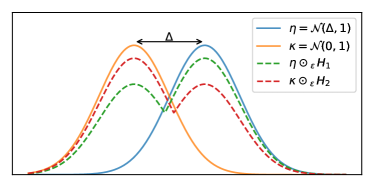
[Plot of corrupted distributions for $\varepsilon=0.2$.][c]        [Plot of $\mathrm{kl}^{\varepsilon}_{\mathcal{G}}$ for $\sigma=1$ and $\varepsilon=0.1$.][c]

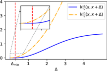
Figure 1: Illustration of the corrupted distributions from Lemma 1 and $\mathrm{kl}^{\varepsilon}_{\mathcal{G}}$. $\mathrm{Supp}(H)$ denotes the support of distribution $H$. $\Delta_{\min}$ is defined in Definition 2.3.

Lemma 1 (Optimal corruption pair)

For $\eta\in\mathcal{P}(\mathbb{R})$, $\kappa\in\mathcal{P}(\mathbb{R})$, and $\varepsilon\in(0,\frac{1}{2})$, $H_{1}$ and $H_{2}$ defined by Equations  (2.2) and (2.3), respectively, are the optimal corruption pair in Equation (2.1), i.e., $(H_{1},H_{2})\in\arg\!\min\left\{{\mathrm{KL}(\eta\odot_{\varepsilon}H,\kappa\odot_{\varepsilon}H^{\prime}):H\in\mathcal{P}(\mathbb{R}),~{}H^{\prime}\in\mathcal{P}(\mathbb{R})}\right\}.$

To prove the above result, we show that the directional derivative (for an appropriate notion in the space of probability measures) of $\mathrm{KL}$ in every direction is non-negative at $(H_{1},H_{2})$. We refer the reader to Section A.2 for a proof of the above result. A similar pair of corruption distributions were considered by Huber (1965) in a hypothesis testing setup.

It follows from Lemma 1 that the optimal corruption pair depends on the two input distributions. In particular, the corruption always stays within the support of the input pair of distributions. For illustration, we present these for the Gaussian-inlier setting, i.e., when both $\eta$ and $\kappa$ are Gaussian distributions with unit variance, in Figure 1. We observe that the sets on which there is corruption are located in the right-tail (respectively left-tail) of the distribution on the left (respectively on the right). These and other interesting properties for Gaussian model with corruption are formally proven in Lemma 3 and Appendix D.2, and will be used later in our analysis.

2.3 The case of Gaussian rewards with known variance

With the above minimisers for the corruption pair for fixed $\eta$ and $\kappa$, we are now left with characterising the optimal $\kappa$ in $\operatorname{KL^{\varepsilon}_{inf}}(\eta,x;\mathcal{L})$. When $\cal L=\cal G$, the collection of all Gaussian distributions with a unit variance, and $\eta\in\cal G$, it follows from Lemma 3 (later in the section) that the optimiser $\kappa\in\cal G$ is the one with mean equal to $x$. Using these results in Theorem 1, we get the simplified lower bound for the Gaussian bandit models, which also holds under time-varying corruption (Remark A.1).

Recall that $m(\mu_{a})$ denotes the mean reward of arm $a$ with distribution $\mu_{a}$.

Proposition 2.2 (Lower bound for Gaussian bandits).

For $\mu\in\mathcal{\mathcal{G}}^{K}$, any uniformly-good algorithm satisfies for any suboptimal arm $a$

$$\liminf\limits_{T\rightarrow\infty}\frac{1}{\log(T)}\left(\sup\limits_{{\bf H}\in\mathcal{P}(\mathbb{R})^{K}}\mathbb{E}_{\mu\odot_{\varepsilon}{\bf H}}\left[{N_{a}(T)}\right]\right)~{}\geq~{}\frac{1}{\mathrm{kl}^{\varepsilon}_{\mathcal{G}}(m(\mu_{a}),m^{*}(\mu))}~{},\quad\text{where }$$

$$\forall x,\!y\!\in\!\mathbb{R},x\!\leq\!y\quad\mathrm{kl}^{\varepsilon}_{\mathcal{G}}(x,y)\!$$ (2.4)

Here, the optimal pair of corruption distributions are given by Lemma 1.

We now state the necessary and sufficient conditions to have a finite lower bound on regret in Gaussian bandits (Proposition 2.2) for a known and fixed $\varepsilon\in\left(0,\frac{1}{2}\right)$. Thus, Lemma 2 states the (necessary and sufficient) conditions to achieve logarithmic regret for Gaussian bandits.

Lemma 2 (Disjoint corruption neighbourhoods)

​ For $\eta\in\mathcal{G}$, $\kappa\in\mathcal{G}$, the following are equivalent:

$${\bf(1)}~{}\forall(H_{1},H_{2})\in\mathcal{P}(\mathbb{R})^{2},~{}\kappa\odot_{\varepsilon}H_{1}\neq\eta\odot_{\varepsilon}H_{2},~{}~{}{\bf(2)}~{}|m(\kappa)-m(\eta)|>2\Phi^{-1}\left(\frac{1}{2(1-\varepsilon)}\right).$$

The condition $(1)$ above states that for any corruption distribution $H_{1}$, there doesn’t exist a distribution $H_{2}$ such that the corrupted distributions $\kappa\odot_{\varepsilon}H_{1}$ and $\eta\odot_{\varepsilon}H_{2}$ are the same, rendering $\mathrm{kl}^{\varepsilon}_{\cal G}(m(\kappa),m(\eta))=0$, i.e., the corruption neighbourhoods (Definition C.1) of $\kappa$ and $\eta$ are disjoint. The lemma above shows that this condition is equivalent to separation in the means of the two Gaussian distributions $\eta$ and $\kappa$. This is also related to the fact that in the presence of corruption, the mean of the true distributions can only be estimated up to an unavoidable error (Appendix C). We postpone the proof of Lemma 2 to Section C.1.

Lemma 2, when combined with Proposition 2.2, implies that a suboptimal condition to ensure logarithmic regret is a separation between the means of the optimal arm and suboptimal arms. This justifies formally introducing the required minimum gap.

Definition 2.3 (Minimum distinction gap under corruption).

$\Delta_{\min}$.

For Gaussian distributions, KL can be expressed using CDF $\Phi$ and PDF $\varphi$ of a standard Gaussian. Moreover, the corrupted KL, viz. $\mathrm{kl}^{\varepsilon}_{\mathcal{G}}$, enjoys nice properties like an almost closed-form expression, shift invariance, differentiability, etc., described in the following lemma.

Lemma 3 (Properties of $\mathrm{kl}^{\varepsilon}_{\mathcal{G}}(x,y)$)

Let $H_{1},H_{2}$ be minimisers in Equation (2.4).

1. The normalisation constants $c_{1}$ and $c_{2}$ are equal, i.e., $c$, and uniquely solve

   $${1}/\left({1-\varepsilon}\right)=c\Phi(\Delta_{-}/2)+\Phi(\Delta_{+}/2),\vspace{-0.25em}$$ (2.5)

   with $\Delta_{+}$, and $\Delta_{-}$.

2. $\mathrm{kl}^{\varepsilon}_{\mathcal{G}}$ has an almost closed-form expression (Equation (D.1)) (up to $c$ defined as in Part (a)). For $0\leq\Delta\leq\Delta_{\min}$, $x\in\mathbb{R}$, $\mathrm{kl}^{\varepsilon}_{\mathcal{G}}(x,x+\Delta)=0$. Moreover, it is invariant, i.e.,

   $$\mathrm{kl}^{\varepsilon}_{\mathcal{G}}(x+\Delta,y)=\mathrm{kl}^{\varepsilon}_{\mathcal{G}}(x,y-\Delta),\quad\text{ for }y\geq x+\Delta.\vspace{-.25em}$$

3. For $x\in\mathbb{R}$ and $\Delta\geq 0$, the function $\Delta\mapsto\mathrm{kl}^{\varepsilon}_{\mathcal{G}}(x,x+\Delta)$ is continuously differentiable. For $\varepsilon>0$ and $\Delta\leq\Delta_{\min}$, ${\partial~{}\mathrm{kl}^{\varepsilon}_{\mathcal{G}}(x,x+\Delta)}/{\partial\Delta}=0$. For $\Delta>\Delta_{\min}$,

   $$\frac{\partial~{}\mathrm{kl}^{\varepsilon}_{\mathcal{G}}(x,x+\Delta)}{\partial\Delta}=\left({1-\varepsilon}\right)\Delta\left({\Phi({\Delta_{+}}/{2})-\Phi({\Delta_{-}}/{2})}\right)>0.$$

They constitute the key properties of the corrupted divergence used in our regret analysis. We refer the reader to Appendix D for a complete proof of Lemma 3, plus other interesting properties of $\mathrm{kl}^{\varepsilon}_{\mathcal{G}}$.

Consequences of Lemma 3. Part (b) shows that there is a flat region below $\Delta=\Delta_{\min}$, where $\mathrm{kl}^{\varepsilon}_{\cal G}(x,x+\Delta)$ equals $0$ (Fig. 1). We use this property in regret analysis of the algorithm for proving fast convergence of the empirical $\mathrm{kl}^{\varepsilon}_{\mathcal{G}}$ to $0$, as well as to avoid certain computations at each step. Part (c) shows that $\mathrm{kl}^{\varepsilon}_{\mathcal{G}}$ is strictly increasing in the second argument for values larger than the first argument. This was used in Proposition 2.2 to conclude that $\operatorname{KL^{\varepsilon}_{inf}}(\eta,x;\mathcal{G})=\mathrm{kl}^{\varepsilon}_{\mathcal{G}}(m(\eta),x)$.

Computational remarks. The normalising constant $c$ from Part (a) implicitly depends on $\varepsilon$ and $\Delta$, and so do $\Delta_{-}$ and $\Delta_{+}$. Here, $\Delta_{-}$ and $\Delta_{+}$ are related to support sets of the optimal corruption pair $H_{1}$ and $H_{2}$ (Lemma 7 in Appendix D). For $\Delta$ converging to $\Delta_{\min}$, $c$ can be shown to converge to $1$ with $\Delta_{-}$ and $\Delta_{+}$ converging to $\Delta_{\min}$. This can be seen from Equation (2.5). In this limit, from Lemma 3(c), it follows that the derivative of $\mathrm{kl}^{\varepsilon}_{\mathcal{G}}$ converges to $0$.

We also note that unlike the classical Gaussian bandit, from Fig. 1 we see that $\mathrm{kl}^{\varepsilon}_{\cal G}(x,x+\Delta)$ is non-convex in $\Delta$, implying that after a point, increasing $\Delta$ does not substantially decrease the number of pulls of suboptimal arms, and hence the regret, in presence of corruption.

3 CRIMED: Algorithm and analysis

In this section, we leverage the lower bound in Proposition 2.2 to propose an algorithm robust to corruption, namely CRIMED. We then give a finite-sample upper bound on the regret of CRIMED, showing its asymptotic optimality for Gaussian bandits with unbounded stochastic corruption. Finally, we explicate the technical novelty of our regret analysis. We discuss an extension of CRIMED for handling model-misspecifications in Appendix F.

3.1 Algorithm design: An IMED-based algorithm with estimated medians

First, we present our algorithm design. For $n\in\mathbbm{N}$ and $a\in[K]$, let $\hat{\mu}_{a}(n)$ denote the empirical distribution constructed using $N_{a}(n)$ samples from arm $a$. We use median of the corrupted observations as an estimator for the mean of underlying reward distributions. This choice is natural in the case of Gaussian distributions, since it is known that the median has the smallest bias due to corruption among all location estimators in a corruption neighbourhood of the Gaussian (ref. Lemma 5 and corresponding discussion in Section C). The fact that we use the median is also closely linked to the symmetry of the Gaussian distribution for which median is the same as mean.

Let $\mathrm{Med}(\cdot)$ denote the median of the input distribution, and define the maximum estimated median at time $n$ as $\mathrm{Med}_{*}(n):=\max_{a}~{}\mathrm{Med}(\hat{\mu}_{a}(n))$. We present CRIMED in Algorithm 1. Note that in Algorithm 1 we introduce a forced exploration for $N_{\min}$ steps, where for $T>0$,

$$N_{\min}$$ (3.1)

Here, $\!s_{\varepsilon}$ is a proxy of the variance of the empirical median from Theorem 3. It converges to a constant, $\!\frac{1}{2\varphi(1)}$, as $\varepsilon\!\rightarrow\!0$. The amount of forced-exploration $N_{\min}$ is $o(s_{\varepsilon}^{2}\log T)$ as $T\!\to\!\infty$. Since we use empirical median as an estimate for the true mean using the corrupted observations, the empirically-optimal arm, or the arm with the maximum estimated mean is defined as $a^{*}(n):=\arg\!\max_{b}~{}\mathrm{Med}(\hat{\mu}_{b}(n))$. Moreover, since for this arm $\mathrm{kl}^{\varepsilon}_{\mathcal{G}}(\mathrm{Med}(\hat{\mu}_{a^{*}(n)}(n))-\Delta_{\min},\mathrm{Med}_{*}(n))=0$, its index is trivial to compute (Lemma 3(b)). For other arms, we use the explicit formulation for $\mathrm{kl}^{\varepsilon}_{\mathcal{G}}$ (Lemma 3(b)), while we compute the constant $c$ using a root-finding algorithm on Equation (2.5).

Input : Horizon $T$, Corruption level $\varepsilon$, $K$

Initialisation phase: Compute $N_{\min}$ using Equation (3.1) and pull every arm $N_{\min}$ times.

for $n\in\left\{{KN_{\min}+1,\dots,T-1,T}\right\}$ do

       Set $\mathrm{Med}_{*}(n)\leftarrow\max_{a}\mathrm{Med}(\hat{\mu}_{a}(n))$, $A_{n}^{*}\in\arg\!\max_{a}\mathrm{Med}(\hat{\mu}_{a}(n))$, $I_{A^{*}_{n}}(n)\leftarrow\log N_{A^{*}_{n}}(n)$.

       Compute, for each arm $a$ different from $A_{n}^{*}$,

$$I_{a}(n)\leftarrow N_{a}(n)\mathrm{kl}^{\varepsilon}_{\mathcal{G}}\left({\mathrm{Med}(\hat{\mu}_{a}(n))-\Delta_{\min},\mathrm{Med}_{*}(n)}\right)+\log N_{a}(n).$$

Pull the arm $A_{n}\in\arg\!\min_{a}I_{a}(n)$.

      

end for

Algorithm 1 CRIMED for unit variance Gaussian bandits

3.2 Theoretical results: Regret upper bound and concentration results

We now present the theoretical guarantees of the proposed algorithm, as well as the refined concentration inequality for median that play a key role in our analysis, and are of independent interest.

Theorem 2 (Finite-sample regret upper bound)

For $\varepsilon\in(0,\frac{1}{2})$ and $\mu\in\mathcal{G}^{K}$ such that for each suboptimal arm $a$, $\Delta_{a}>\Delta_{\min}$, CRIMED satisfies

$$\mathbb{E}[N_{a}(T)]\leq N_{\min}+\frac{\log(T)}{\mathrm{kl}^{\varepsilon}_{\mathcal{G}}\left({m(\mu_{a}),m^{*}(\mu)}\right)-2\delta\left(\Delta_{a}+\delta+\Delta_{\min}\right)}+O((\log T)^{0.99}),$$

where $m^{*}(\mu)=\max_{a}m(\mu_{a})$, and $\delta^{2}:=\left({\log(1+\log(1+\log T))}\right)^{-1}$.

The exact $O((\log T)^{0.99})$ term can be found in Equation (E.5) in the Appendix E. We believe that the forced exploration for $N_{\min}$ steps is an artefact of the proof, and is needed in our analysis to handle the difficulties due to corruption. Indeed, in Section 4, we numerically compare CRIMED and an aggressive version with $N_{\min}=1$, called CRIMED*, and observe a smaller regret for CRIMED*.

Corollary 3.1 (Asymptotic optimality).

For $\varepsilon\in(0,\frac{1}{2})$ and $\mu\in\mathcal{G}^{K}$ such that for each suboptimal arm $a$, $\Delta_{a}>\Delta_{\min}$, CRIMED is asymptotically optimal, i.e., $\limsup\limits_{T\rightarrow\infty}\frac{\mathbb{E}\left[{N_{a}(T)}\right]}{\log T}\leq\frac{1}{\mathrm{kl}^{\varepsilon}_{\mathcal{G}}(m(\mu_{a}),m^{*}(\mu))}.$

The proof of Theorem 2, which we detail in Appendix E, proceeds by controlling the probability of selecting a suboptimal arm $a$ at each step $n$. CRIMED pulls arm $a$ at time $n$ if its index $I_{a}(n)$ is the smallest. Thus, the probability of pulling an arm can be bounded by controlling the deviations of $\mathrm{kl}^{\varepsilon}_{\mathcal{G}}$ evaluated on the empirical estimates. This in turn is related to the probability of deviation of the empirical estimates themselves. In Theorem 3, we prove a new concentration result for the empirical median, which we leverage to prove that the regret of CRIMED is well controlled. Later, in Lemma 4, we present the concentration results for the $\mathrm{kl}^{\varepsilon}_{\mathcal{G}}$ evaluated at the empirical estimates. Given $n$ samples $X_{1},\dots,X_{n}$, $\mathrm{Med}(X^{n}_{1})$ denotes the empirical median. This can be alternatively seen as $\mathrm{Med}(\hat{P}_{n})$, where $\hat{P}_{n}$ denotes their empirical distribution of $X_{1},\dots,X_{n}$.

Theorem 3 (Concentration of median for corrupted Gaussians)

Let $X_{1},\dots,X_{n}$ be independent samples such that $X_{i}\sim\mathcal{N}(m,1)\odot_{\varepsilon}H_{i}$, for $H_{i}\in\mathcal{P}(\mathbb{R})$, and let $\varepsilon<\frac{1}{2}$. For $y\in[0,1]$,

$$\mathbb{P}\left(\mathrm{Med}(X_{1}^{n})-m\geq\frac{\Delta_{\min}}{2}+y\right)\vee\mathbb{P}\left(\mathrm{Med}(X_{1}^{n})-m\leq-\frac{\Delta_{\min}}{2}-y\right)\leq 2\exp\left(\frac{-ny^{2}}{s_{\varepsilon}^{2}}\right).$$

We remark that Theorem 3 does not require i.i.d. samples. In particular, the corruption distribution is allowed to be time-varying. Further, observe from Equation (3.1) that when $\varepsilon$ goes to $0$, $s_{\varepsilon}$ goes to $\frac{1}{2\varphi(1)}$. On the other hand, when $\varepsilon$ goes to $\frac{1}{2}$, $\varphi(\frac{\Delta_{\min}}{2}+1)$ goes to $0$, hence $s_{\varepsilon}$ goes to $\infty$, and we get a trivial bound in the theorem. In particular, our bound adapts to $\varepsilon$. We refer the reader to Appendix E.5 for a proof of the theorem.

Remark 3.2 (A refined concentration result).

Theorem 3 is an improvement over the concentration in Altschuler et al. (2019, Lemma 7) in which the variance term does not depend on $\varepsilon$. Furthermore, Theorem 3 allows for an $\varepsilon$ that is arbitrarily close to $\frac{1}{2}$, which is an improvement over the existing bounds for robust mean estimators featuring an upper limit on $\varepsilon$ away from $\frac{1}{2}$. For example, $\varepsilon\leq\frac{1}{7}$ in (Wang and Ramdas, 2023, Theorem 2), and $\varepsilon\leq\frac{1}{15}$ in (Altschuler et al., 2019, Theorem 18).

Using Theorem 3 and properties of $\mathrm{kl}^{\varepsilon}_{\mathcal{G}}$, we prove the following concentration result.

Lemma 4 (Concentration of $\mathrm{kl}^{\varepsilon}_{\mathcal{G}}$.)

Let $\delta>0$, $x\in\mathbb{R}$. Let $X_{1},\dots,X_{n}$ be $n$ independent samples such that $X_{i}\sim\mathcal{N}(m_{a},1)\odot_{\varepsilon}H_{i}$, for $H_{i}\in\mathcal{P}(\mathbb{R})$.

1. For $y\in[0,1]$, with probability at least $1-2\exp\left(-ny^{2}/s_{\varepsilon}^{2}\right)$,

   $$\mathrm{kl}^{\varepsilon}_{\mathcal{G}}\left(\mathrm{Med}(X^{n}_{1})-\frac{\Delta_{\min}}{2},m_{a}-\delta\right)\leq\left(y-\delta\right)_{+}\left(|y-\delta|+\frac{\Delta_{\min}}{2}\right).$$

2. For $m_{b}>m_{a}+\Delta_{\min}$ and $y\in[0,1]$, with probability at least $1-2\exp\left(-ny^{2}/s_{\varepsilon}^{2}\right)$,

   $$\mathrm{kl}^{\varepsilon}_{\mathcal{G}}\left(m_{a},m_{b}\right)-\mathrm{kl}^{\varepsilon}_{\mathcal{G}}\left(\mathrm{Med}(X^{n}_{1})-\frac{\Delta_{\min}}{2},m_{b}\right)\leq y(m_{b}-m_{a}+y+\Delta_{\min}).\vspace{-0.25em}$$

A useful thresholding. For $y\in[0,\delta)$ the probability of $\mathrm{kl}^{\varepsilon}_{\mathcal{G}}(\mathrm{Med}(X^{n}_{1})-\frac{\Delta_{\min}}{2},m_{a}-y)$ being $0$ is strictly positive, from Lemma 4(a). This contrasts with the uncorrupted-Gaussian setting, for which this is a zero probability event, except when $y=0$. We extensively use this key property in the proof of Theorem 2, which follows from the thresholding property that $\mathrm{kl}^{\varepsilon}_{\mathcal{G}}\left(x,x+\Delta\right)\!=\!0$ holds for any $\Delta\!\leq\!\Delta_{\min}$. Specifically, the probability of being $0$ coincides with that for $m_{a}-y-\mathrm{Med}(X^{n}_{1})\leq\frac{\Delta_{\min}}{2}$. We refer the reader to Appendix E.6 for a proof of the lemma.

Challenges in the regret analysis. To prove Theorem 2, we modify the proof for the regret bound of Honda and Takemura (2015). The major difference arises from the fact that Theorem 3 does not allow us to reach arbitrarily large level of confidence, i.e. with $y\leq 1$, the probability in Theorem 3 cannot be smaller than $\exp(-\Omega(n))$. This implies that very large deviation of the median do not imply very small probabilities. This is a known limitation of robust estimators (Devroye et al., 2016). As a consequence, we change the decomposition of the bad event $A_{n}=a$ to also include an event on which the deviation of the $\mathrm{kl}^{\varepsilon}_{\mathcal{G}}$ is large.

We decompose the event $A_{n}=a$ as a union of three disjoint events. (i) $E_{n}(a)$: when the suboptimal arm is not well estimated. (ii) $F_{n}(a)$: when the optimal arm is not well estimated and $G_{n}(a)$ when $\mathrm{kl}^{\varepsilon}_{\mathcal{G}}$ has large deviations (ref. Lemma 10 for formal definitions). We highlight that Lemma 4(a) with $y=\delta$, i.e. the fast concentration to $0$, is specifically used to control the probabilities of events $F_{n}(a)$ and $G_{n}(a)$. (iii) Event $G_{n}(a)$ is further controlled thanks to the forced-exploration mechanism. Indeed, we observe that even refined concentration such as anytime concentration might only improve the lower order terms in the regret upper bound, but are not sufficient to control $G_{n}(a)$.

4 Experimental illustration

In this section, we numerically illustrate the efficiency of our algorithm. The computation of CRIMED indices depends on the threshold $c$, that we evaluate using Equation (2.5) and the default scipy (Virtanen et al., 2020) root-finding algorithm. We consider arm distributions as $\mathcal{N}(m_{a},\sigma_{a}^{2})$, i.e., Gaussian inliers. The corruption distributions (outliers) are of form $\mathcal{N}(m_{o},\sigma_{o}^{2})$ in Setting $1$ and $2$, and standard Cauchy in Setting $3$. Table below details the parameters used. Arm $3$ is optimal.

Parameters	Horizon	$\sigma_{a}$	means arms $m_{a}$	$\varepsilon$	medians outliers $m_{b}$	$\sigma_{o}$ outliers
Setting 1	10,000	0.5	[0.8, 0.9, 1]	0.01	[1, 1, 0.8]	1
Setting 2	10,000	0.5	[0.8, 0.9, 1]	0.01	[10, 10, -20]	1
Setting 3	10,000	0.5	[0.8, 0.9, 1]	0.01	[10, 10, -20]	$\infty$

Setting $1$ corresponds to a mild corruption, in which the corrupted distribution of arm $3$ still has the largest mean of $0.98$. In Setting $2$, the corruption causes a change in the order of the arms (arm $2$ is optimal according to the corrupted distributions). Hence, robustness is needed to identify correctly the optimal arm. In Setting $3$, the outliers are heavy-tailed. We compare $4$ algorithms: CRIMED (Algorithm 1) with $N_{\min}$ set to Equation (3.1), CRIMED*, an aggressive version of CRIMED with $N_{\min}$ set to $1$, IMED is the same as CRIMED* but in which there is no corruption ($\varepsilon=0$) and the means are estimated using the empirical mean, and finally RobustUCB  (Basu et al., 2022).

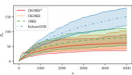
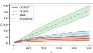
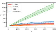
Figure 2: Cumulative regret for $100$ repetitions on Settings $1$ (left), $2$ (middle), and $3$ (right). Solid lines represent the means and shaded area are $90\%$ percentile intervals.

Figure 2 illustrates that all the algorithms, except IMED, feature a logarithmic regret. IMED incurs a linear regret in large-corruption settings (Settings $2$, $3$). On the other hand, CRIMED and CRIMED* perform comparably, and they are both performing better than RobustUCB. We also observe no significant difference in performance when the corruptions are heavy-tailed vs Gaussian.

5 Discussion and open questions

We studied a variant of the stochastic multi-armed bandits with unbounded stochastic corruption and analysed the behaviour of the KL divergence within a corruption neighbourhood in details. This served as the foundation for the proposed algorithm CRIMED, that asymptotically achieves this lower bound for Gaussian bandits. We developed a new concentration result for median allowing CRIMED to tackle corruption proportion up to $\frac{1}{2}$, which was not possible with the existing algorithms. We discussed a modification of CRIMED to handle misspecifications in Gaussian model.

We believe that the Gaussian reward assumption is not essential, and we believe it is possible to generalise these results to at least symmetric, unimodal distributions. Generalisation to non-symmetric and possibly non-parametric inliers is likely to be much more challenging. This is because in the non-symmetric case, robust estimators approximate location parameters that may be far from the mean and we have to trade off between the error due to corruption and the error due to asymmetry. This requires the study of a non-trivial trade-off between robustness and asymptotic distance to the mean, which we leave as an open question.

This work commenced when S. Agrawal was a PhD student at TIFR, Mumbai, India. S. Agrawal acknowledges support from the Department of Atomic Energy, Government of India, under project no. RTI4001. This work has also been supported by the French Ministry of Higher Education and Research, the Hauts-de-France region, Inria, the MEL, the I-Site ULNE regarding project R-PILOTE-19-004-APPRENF, and the Inria A.Ex. SR4SG project. D. Basu, O.-A. Maillard, and T. Mathieu acknowledge the Inria-Kyoto University Associate Team “RELIANT” for supporting the project. D. Basu also acknowledges the ANR JCJC grant for the REPUBLIC project (ANR-22-CE23-0003-01). Additionally, S. Agrawal acknowledges support from the Sarojini Damodaran Fellowship and the Google PhD Fellowship in Machine Learning.

Appendix A Proofs for results in Section 2.1 and Section 2.2: Lower bound and hardest corruption pair

Remark A.1.

Observe that

$$\sup\limits_{{\bf H_{T}}\in\mathcal{P}(\mathbb{R})^{T\times K}}\mathbb{E}_{\mu\odot_{\varepsilon}{\bf H_{T}}}\left[{N_{a}(T)}\right]\geq\sup\limits_{{\bf H}\in\mathcal{P}(\mathbb{R})^{K}}\mathbb{E}_{\mu\odot_{\varepsilon}{\bf H}}\left[{N_{a}(T)}\right],$$

where $\bf H_{T}$ is a $T\times K$ matrix of corruption distributions with row $n$ being ${\bf H}_{n}$, the vector of corruption distributions at time $n$. Furthermore, on the rhs in the above inequality, we assume that the corruption distributions associated with each arm are same across time. Below, we show that the lower bound for this simpler setting where the corruption doesn’t change with time. Since the lower bound for fixed $H$ across time will only be smaller, this then proves that the same lower bound holds even for the more general setting considered in this work that allows for time-varying corruption.

A.1 Proof of Theorem 1

Let the given bandit instance be denoted by $\mu\in\mathcal{L}^{K}$ and for $a\in[K]$ and let $\left\{{X_{a,i}}\right\}_{a,i}$, for $a\in[K],i\in\left\{{1,\dots,N_{a}(T)}\right\}$ denote the $N_{a}(T)$ corrupted observations from arm $a$ till time $T$. Under the instance $\mu$ with the corruption distributions ${\bf H}=\left\{{H_{1},\dots,H_{K}}\right\}$, the likelihood of observing the samples, denoted by $L_{\mu,\bf H}$, is

$$L_{\mu,\bf H}=\prod\limits_{a=1}^{K}\prod\limits_{i=1}^{N_{a}(T)}\left({(1-\varepsilon)\mu_{a}(X_{a,i})+\varepsilon H_{a}(X_{a,i})}\right)=\prod\limits_{a=1}^{K}\prod\limits_{i=1}^{N_{a}(T)}\mu_{a}\odot_{\varepsilon}H_{a}(X_{a,i}).$$

Without loss of generality, we assume that arm $1$ is the unique optimal arm in $\mu$ and establish the lower bound for the sub-optimal arm $2$. To this end, consider an alternative bandit instance, $\nu=(\nu_{1},\dots,\nu_{K})$, where, $\nu_{b}\in\cal L$ for each $b\in[K]$, for $b\neq 2$, $\nu_{b}=\mu_{b}$, and $m(\nu_{2})\geq m^{*}(\mu)$. Clearly, $m^{*}(\nu)\geq m^{*}(\mu)$. The likelihood of observing samples under $\nu$ with corruption distributions ${\bf H}^{\prime}=\left\{{H^{\prime}_{1},\dots,H^{\prime}_{K}}\right\}$, denoted by $L_{\nu,\bf H^{\prime}}$ is given by

$$L_{\nu,\bf H^{\prime}}=\prod\limits_{a=1}^{K}\prod\limits_{i=1}^{N_{a}(T)}\nu_{a}\odot_{\varepsilon}H^{\prime}_{a}(X_{a,i}).$$

Writing the log-likelihood ratio,

$$LL_{T}=\sum\limits_{a=1}^{K}\sum\limits_{i=1}^{N_{a}(T)}\log\left({\frac{\mu_{a}\odot_{\varepsilon}H_{a}}{\nu_{a}\odot_{\varepsilon}H^{\prime}_{a}}(X_{a,i})}\right).$$

Taking average with respect to $\mu\odot_{\varepsilon}\bf H$, we get

$$\mathbb{E}_{\mu\odot_{\varepsilon}\bf H}\left[{LL_{T}}\right]=\sum\limits_{a=1}^{K}\mathbb{E}_{\mu\odot_{\varepsilon}\bf H}\left[{N_{a}(T)}\right]\mathrm{KL}(\mu_{a}\odot_{\varepsilon}H_{a},\nu_{a}\odot_{\varepsilon}H^{\prime}_{a}).$$

Informally, let $\mathcal{F}_{t}$ be the $\sigma-$algebra generated by the randomness of the algorithm and the observations up to time $t$ (see (Lattimore and Szepesvári, 2020, Chapter 4) for formal introduction to stochastic multi-armed bandits). An application of the data-processing inequality (see, Kaufmann et al. (2016); Garivier et al. (2019)) gives that for any $\mathcal{F}_{T}$ measurable event $\mathcal{E}_{T}$,

$$\sum\limits_{a=1}^{K}\mathbb{E}_{\mu\odot_{\varepsilon}\bf H}\left[{N_{a}(T)}\right]\mathrm{KL}(\mu_{a}\odot_{\varepsilon}H_{a},\nu_{a}\odot_{\varepsilon}H^{\prime}_{a})\geq d\left({\mu_{a}\odot_{\varepsilon}H_{a}(\mathcal{E}_{T}),\nu_{a}\odot_{\varepsilon}H^{\prime}_{a}(\mathcal{E}_{T})}\right),$$

where for $x\in(0,1)$ and $y\in(0,1)$, $d(x,y)$ denotes the $\mathrm{KL}$ divergence between Bernoulli distributions with the given means. Since the r.h.s. above is true for all events $\mathcal{E}_{T}$ that are $\mathcal{F}_{T}$ measurable, optimizing over them we get

$$\sum\limits_{a=1}^{K}\mathbb{E}_{\mu\odot_{\varepsilon}\bf H}\left[{N_{a}(T)}\right]\mathrm{KL}(\mu_{a}\odot_{\varepsilon}H_{a},\nu_{a}\odot_{\varepsilon}H^{\prime}_{a})\geq\sup\limits_{\mathcal{E}_{T}\in\mathcal{F}_{T}}~{}d\left({\mu_{a}\odot_{\varepsilon}H_{a}(\mathcal{E}_{T}),\nu_{a}\odot_{\varepsilon}H^{\prime}_{a}(\mathcal{E}_{T})}\right).$$

Taking infimum over the corruptions ${\bf H}\in{\mathcal{P}(\mathbb{R})}^{K}$ and ${\bf H^{\prime}}\in{\mathcal{P}(\mathbb{R})}^{K}$ on both sides, the above inequality implies

$$\inf\limits_{\bf H,\bf H^{\prime}}~{}\sum\limits_{a=1}^{K}~{} \mathbb{E}_{\mu\odot_{\varepsilon}\bf H}\left[{N_{a}(T)}\right]\mathrm{KL}(\mu_{a}\odot_{\varepsilon}H_{a},\nu_{a}\odot_{\varepsilon}H^{\prime}_{a})$$

$$\geq\inf\limits_{\bf H,\bf H^{\prime}}~{}\sup\limits_{\mathcal{E}_{T}\in\mathcal{F}_{T}}~{}d\left({\mu_{a}\odot_{\varepsilon}H_{a}(\mathcal{E}_{T}),\nu_{a}\odot_{\varepsilon}H^{\prime}_{a}(\mathcal{E}_{T})}\right).$$ (A.1)

Since for every $\bf H$, $\bf H^{\prime}$ with $H^{\prime}_{b}=H_{b}$ for all $b\in[K]$ and $b\neq 2$ is a feasible candidate for $\bf H^{\prime}$, the infimum in the l.h.s. above is at most

$$\left({\sup\limits_{\bf H}~{}\mathbb{E}_{\mu\odot_{\varepsilon}\bf H}\left[{N_{2}(T)}\right]}\right)\left({\inf\limits_{H_{2},H^{\prime}_{2}}\mathrm{KL}(\mu_{2}\odot_{\varepsilon}H_{2},\nu_{2}\odot_{\varepsilon}H^{\prime}_{2})}\right).$$ (A.2)

Now, following along the arguments in Kaufmann et al. (2016) for the classical regret-minimization setting without corruption, we first choose

$$\mathcal{E}_{T}=\left\{{N_{1}(T)\leq T-\sqrt{T}}\right\}.$$

Then, we obtain by a simple application of Markov’s inequality

$$\mathbb{P}_{\mu\odot_{\varepsilon}\bf H}\left({\mathcal{E}_{T}}\right)=\mathbb{P}_{\mu\odot_{\varepsilon}\bf H}\left({T-N_{1}(T)\geq\sqrt{T}}\right)\leq\frac{\sum\limits_{a\neq 1}\mathbb{E}_{\mu\odot_{\varepsilon}\bf H}\left[{N_{a}(T)}\right]}{\sqrt{T}}=:P^{\bf H}_{T},$$

and

$$\mathbb{P}_{\nu\odot_{\varepsilon}\bf H^{\prime}}\left({\mathcal{E}^{c}_{T}}\right)=\mathbb{P}_{\nu\odot_{\varepsilon}\bf H^{\prime}}\left({N_{1}(T)\geq T-\sqrt{T}}\right)\leq\frac{\sum\limits_{a\neq 2}\mathbb{E}_{\nu\odot_{\varepsilon}\bf H^{\prime}}\left[{N_{a}(T)}\right]}{T-\sqrt{T}}=:(Q^{\bf H^{\prime}}_{T})^{c}.$$

Next, recall that the algorithm under consideration is uniformly-good (see Definition 2.1). This implies

$$\sup\limits_{\bf H}~{}\mathbb{P}_{\mu\odot_{\varepsilon}\bf H}\left({\mathcal{E}_{T}}\right)\leq P_{T}:=\sup\limits_{H}~{}P^{H}_{T}\xrightarrow{T\rightarrow\infty}{0},$$

and

$$\sup\limits_{\bf H^{\prime}}~{}\mathbb{P}_{\nu\odot_{\varepsilon}\bf H^{\prime}}\left({\mathcal{E}^{c}_{T}}\right)\leq Q^{c}_{T}:=\sup\limits_{\bf H^{\prime}}~{}(Q^{\bf H^{\prime}}_{T})^{c}\xrightarrow{T\rightarrow\infty}{0}.$$

Clearly, for a fixed $\bf H$ and $\bf H^{\prime}$, from the monotonicity of $d(\cdot,\cdot)$ in its arguments, it holds

$$d\left({\mathbb{P}_{\mu\odot_{\varepsilon}\bf H}\left({\mathcal{E}_{T}}\right),\mathbb{P}_{\nu\odot_{\varepsilon}\bf H^{\prime}}\left({\mathcal{E}_{T}}\right)}\right) \geq d\left(\sup\limits_{\bf H}\mathbb{P}_{\mu\odot_{\varepsilon}\bf H}\left({\mathcal{E}_{T}}\right),1-\sup\limits_{\bf H^{\prime}}\mathbb{P}_{\nu\odot_{\varepsilon}\bf H^{\prime}}\left({\mathcal{E}^{c}_{T}}\right)\right)$$

$$\geq d(P_{T},Q_{T}).$$ (A.3)

Using (A.2) and (A.1) in (A.1), we get

$$\left({\sup\limits_{\bf H}~{}\mathbb{E}_{\mu\odot_{\varepsilon}\bf H}\left[{N_{2}(n)}\right]}\right)\left({\inf\limits_{H_{2},H^{\prime}_{2}}~{}\mathrm{KL}(\mu_{2}\odot_{\varepsilon}H_{2},\nu_{2}\odot_{\varepsilon}H^{\prime}_{2})}\right)\geq d(P_{T},Q_{T}).$$ (A.4)

Next, we consider the following relation

$$\lim\limits_{T\rightarrow\infty}\frac{d\left({P_{T},Q_{T}}\right)}{\log T}=\lim\limits_{T\rightarrow\infty}\frac{1}{\log T}\log\frac{1}{Q^{c}_{T}}\geq\lim\limits_{T\rightarrow\infty}\frac{1}{\log T}\log\frac{T-\sqrt{T}}{\sup\limits_{\bf H^{\prime}}\sum\limits_{a\neq 2}\mathbb{E}_{\nu\odot_{\varepsilon}\bf H^{\prime}}\left[{N_{a}(T)}\right]}.$$

We observe that the r.h.s. above equals

$$\lim\limits_{T\rightarrow\infty}\left({1+\frac{\log\left({1-\frac{1}{\sqrt{T}}}\right)}{\log T}-\frac{\log\left({\sup\limits_{\bf H^{\prime}}\sum\limits_{a\neq 2}\mathbb{E}_{\nu\odot_{\varepsilon}\bf H^{\prime}}\left[{N_{a}(T)}\right]}\right)}{\log T}}\right),$$

which in turns equals $1$. Thus, we have obtained

$$\lim\limits_{T\rightarrow\infty}\frac{d\left({P_{T},Q_{T}}\right)}{\log T}\geq 1.$$

Using this in Equation (A.4),

$$\liminf\limits_{T\rightarrow\infty}\frac{\left({\sup\limits_{\bf H}~{}\mathbb{E}_{\mu\odot_{\varepsilon}\bf H}\left[{N_{2}(T)}\right]}\right)}{\log T}\geq\frac{1}{{\inf\limits_{H_{2},H^{\prime}_{2}}~{}\operatorname{KL^{\varepsilon}_{inf}}(\mu_{2}\odot_{\varepsilon}H_{2},\nu_{2}\odot_{\varepsilon}H^{\prime}_{2})}}.$$

Since the above inequality is true for all the alternative bandit instances $\nu\in\mathcal{L}^{K}$ with $m(\nu_{2})\geq m^{*}(\mu)$, we optimize over these to get

$$\liminf\limits_{T\rightarrow\infty}\frac{\left({\sup\limits_{\bf H}~{}\mathbb{E}_{\mu\odot_{\varepsilon}\bf H}\left[{N_{2}(T)}\right]}\right)}{\log T}\geq\frac{1}{\operatorname{KL_{inf}}(\mu_{2},m^{*}(\mu);\cal L)},$$

where $\operatorname{KL^{\varepsilon}_{inf}}(\mu_{2},m^{*}(\mu);\cal L)$ equals

$$\inf\left\{{\mathrm{KL}(\mu_{2}\odot_{\varepsilon}H_{2},\nu_{2}\odot_{\varepsilon}H^{\prime}_{2}):~{}\nu_{2}\in\mathcal{L},~{}m(\nu_{2})\geq m^{*}(\mu),~{}H_{2}\in\mathcal{P}(\mathbb{R}),~{}H^{\prime}_{2}\in\mathcal{P}(\mathbb{R})}\right\}.$$

A.2 Proof of Lemma 1

Given $\eta\in\cal L$ and $\kappa\in\cal L$, we will show that $H_{1}$ and $H_{2}$ satisfying (2.2) and (2.3) are optimal for $\operatorname{KL^{\varepsilon}_{inf}}$, for a fixed $\kappa$. To this end, consider any alternative corruption distributions, $H^{\prime}_{1}\in\mathcal{P}(\mathbb{R})$ and $H^{\prime}_{2}\in\mathcal{P}(\mathbb{R})$. For $t\in(0,1)$, define

$$H_{i,t}=(1-t)H_{i}+tH^{\prime}_{i},\quad\text{ for }i\in\left\{{1,2}\right\},$$

and

$$J_{H^{\prime}_{1},H^{\prime}_{2}}(t)=\frac{1}{\varepsilon}\mathrm{KL}(\eta\odot_{\varepsilon}H_{1,t},\kappa\odot_{\varepsilon}H_{2,t}).$$

To prove the lemma, we show that $J_{H^{\prime}_{1},H^{\prime}_{2}}$ is a convex function that is minimized at $t=0$. To see this,

$$\frac{\mathrm{d}J_{H^{\prime}_{1},H^{\prime}_{2}}}{\mathrm{d}t}(t)= \int\log\frac{\mathrm{d}\eta\odot_{\varepsilon}H_{1,t}}{\mathrm{d}\kappa\odot_{\varepsilon}H_{2,t}}(x)\left({\mathrm{d}H^{\prime}_{1}-\mathrm{d}H_{1}}\right)(x)$$

$$\qquad-\int\mathrm{d}\eta\odot_{\varepsilon}H_{1,t}(x)\left(\frac{\left({\mathrm{d}H^{\prime}_{2}-\mathrm{d}H_{2}}\right)}{\mathrm{d}\kappa\odot_{\varepsilon}H_{2,t}}(x)-\frac{\left({\mathrm{d}H^{\prime}_{1}-\mathrm{d}H_{1}}\right)}{\mathrm{d}\eta\odot_{\varepsilon}H_{1,t}}(x)\right)$$

$$= \int\log\frac{\mathrm{d}\eta\odot_{\varepsilon}H_{1,t}}{\mathrm{d}\kappa\odot_{\varepsilon}H_{2,t}}(x)\left({\mathrm{d}H^{\prime}_{1}-\mathrm{d}H_{1}}\right)(x)-\int\frac{\mathrm{d}\eta\odot_{\varepsilon}H_{1,t}}{\mathrm{d}\kappa\odot_{\varepsilon}H_{2,t}}(x)\left(\mathrm{d}H^{\prime}_{2}-\mathrm{d}H_{2}\right)(x),$$

where the last equality follows from the fact that $H_{1}$ and $H_{1}^{\prime}$ both integrate to $1$. Differentiating again with respect to $t$,

$$\frac{{\mathrm{d}}^{2}J_{H^{\prime}_{1},H^{\prime}_{2}}}{\mathrm{d}t^{2}}(t)= \int\left(\frac{\mathrm{d}H_{1}^{\prime}-\mathrm{d}H_{1}}{\sqrt{\mathrm{d}\eta\odot_{\varepsilon}H_{1,t}}}-\sqrt{\mathrm{d}\eta\odot_{\varepsilon}H_{1,t}}\frac{\mathrm{d}H_{2}^{\prime}-\mathrm{d}H_{2}}{\mathrm{d}\kappa\odot_{\varepsilon}H_{2,t}}\right)^{2}$$

$$\geq 0,$$

proving the convexity of $J_{H^{\prime}_{1},H^{\prime}_{2}}$ for any $H_{1}^{\prime},H_{2}^{\prime}$. Thus, it suffices to prove that its derivative is non-negative at $t=0$.

We now define the sets

$$A:=\left\{{x:~{}\frac{d\eta}{\mathrm{d}\kappa}(x)<c_{1}}\right\}\quad\text{ and }\quad D:=\left\{{x:~{}\frac{\mathrm{d}\eta}{\mathrm{d}\kappa}(x)>\frac{1}{c_{2}}}\right\}.$$ (A.5)

Then,

$$\frac{\mathrm{d}J_{H^{\prime}_{1},H^{\prime}_{2}}}{\mathrm{d}t}(0) =\int\limits_{A}\log\left({c_{2}}\right)\left({\mathrm{d}H^{\prime}_{1}-\mathrm{d}H_{1}}\right)(x)+\int\limits_{A^{c}\cap D^{c}}\log\frac{\mathrm{d}\eta}{\mathrm{d}\kappa}(x)\mathrm{d}H^{\prime}_{1}(x)+\int\limits_{D}\log\frac{1}{c_{1}}\mathrm{d}H^{\prime}_{1}(x)$$

$$\qquad\qquad-\int\limits_{A}c_{2}\mathrm{d}H^{\prime}_{2}(x)-\int\limits_{A^{c}\cap D^{c}}\frac{\mathrm{d}\eta}{\mathrm{d}\kappa}(x)\mathrm{d}H^{\prime}_{2}(x)-\int\limits_{D}\frac{1}{c_{1}}\left({\mathrm{d}H^{\prime}_{2}-\mathrm{d}H_{2}}\right)(x)$$

$$\geq\log c_{2}\left({1-H_{1}(A)}\right)-\frac{1}{c_{1}}\left({1-H_{2}(D)}\right)$$

$$=0,$$

where the last equality follows from the facts that $H^{\prime}_{1}$ and $H^{\prime}_{2}$ have supports equal to $A$ and $D$, respectively, and integrate to $1$.

Remark A.2.

Observe that Equation (2.2) and (2.3) implicitly define the probability measures $H_{1}$ and $H_{2}$. To see this, we first argue that $H_{1}$ is non-negative. Recall that

$$\mathrm{d}(\eta\odot_{\varepsilon}H_{1})=(1-\varepsilon)\mathrm{d}\eta+\varepsilon\mathrm{d}H_{1}.$$

From (2.2) it is clear that $\mathrm{d}H_{1}(x)=0$ for $\frac{\mathrm{d}\eta}{\mathrm{d}\kappa}\geq c_{1}$. Thus, $H_{1}$ is supported only on the complement set, where it is non-negative by choice of $c_{1}$. Next, since $\mathrm{d}(\eta\odot_{\varepsilon}H_{1})$ integrates to $1$ (by choice of $c_{1}$) and so does $\eta$, $H_{1}$ too integrates to $1$. One can similarly argue that $H_{2}$ defined by Equation (2.3) is a probability measure.

Appendix B Discussion on the knowledge of $\varepsilon$ and an impossibility result

We note that in the current work, we do not require the knowledge of the precise value of corruption probability $\varepsilon$. Instead, the knowledge of an upper bound on $\varepsilon$ is sufficient. In this section, we will show that without the knowledge of $\varepsilon$, no uniformly-good algorithm can achieve logarithmic regret (Remark B.1).

We remind that this is also a standard assumption in the robust statistics literature. On a related note, Wang and Ramdas (2023, Remark 3) mention as an open problem whether it is possible to construct confidence intervals using corrupted samples without the knowledge of $\varepsilon$ (or a bound on it). In this section, we provide a negative answer to this question as well.

Our approach is to relate the problem of constructing anytime-valid confidence intervals in presence of corruption to a specific sequential hypothesis testing problem using corrupted data, which can be formulated as the best-arm identification (BAI) problem with corruptions in the multi-armed bandit framework. We then use the machinery from the proof of Theorem 1 to arrive at a lower bound for this problem in terms of $\operatorname{KL^{\varepsilon}_{inf}}$, defined in Equation (2.1). We show that if a bound on $\varepsilon$ is not known, then $\operatorname{KL^{\varepsilon}_{inf}}=0$, rendering the BAI problem un-learnable, hence, the impossibility for existence of a sequential test, and hence, impossibility for existence of non-trivial anytime confidence intervals. The approach for proving impossibility result for BAI is reminiscent of a similar negative result for classical BAI in bandits with heavy-tailed distributions (uncorrupted setting), proven in  (Agrawal et al., 2020, Theorem 3).

For $\delta>0$ and a collection $\cal L$ of probability measures, we only prove the negative result for constructing an any-time valid upper bound that holds with probability at least $1-\delta$, using samples generated from a corruption neighbourhood (Definition C.1) of a distribution $\mu_{1}\in\cal L$. Symmetric arguments (including a symmetric sequential test) give a corresponding negative result for the lower bound that holds with probability at least $1-\delta$. We now introduce the specific sequential test for this.

Sequential setting (hypothesis testing) of interest.

Consider the problem of testing whether the mean of a distribution $\mu_{1}\in\cal L$ is below a given threshold $\zeta$ in a $\delta$-correct framework. To be more specific, let $m(\mu_{1})$ denote its mean, and let $m(\mu_{1})<\zeta$ (unknown to the algorithm). The algorithm can generate samples from $\mu_{1}$. However, on doing so, it observes the true sample with probability $1-\varepsilon$, and receives a sample from an arbitrary corruption distribution with the remaining $\varepsilon$ probability, i.e., it observes samples from an $\varepsilon$ corruption neighbourhood of $\mu_{1}$. In presence of $\varepsilon$ corruption, the goal of the algorithm is to generate finite samples (possibly random number of samples, depending on observations made), and declare that $m(\mu_{1})<\zeta$ with probability at least $1-\delta$. While ensuring this $\delta$-correctness property, the algorithm’s goal is also to minimise its expected stopping time. Let us denote the $\delta$-correct algorithm for this problem by $\mathcal{A}(\delta,\zeta)$.

Equivalence of $\delta$-correct anytime-valid upper bound and sequential test described above.

Observe that given a $\delta$-correct algorithm for the above described problem, $\mathcal{A}(\delta,\zeta)$, one can construct an anytime-valid upper bound on the true mean for $\mu_{1}$ that holds with probability at least $1-\delta$ using $\varepsilon$-corrupted samples as follows: at any time $n$, define the set

$$U_{n}:=\left\{{\zeta:\mathcal{A}(\delta,\zeta)\text{ has not stopped in $n$ samples}}\right\}.$$

Then, $U_{n}$ is an anytime-valid upper bound on $m(\mu_{1})$ that holds with probability at least $1-\delta$. The reverse implication also holds, i.e., given any sequence of $\delta$-correct anytime-valid upper bound on $m(\mu_{1})$ constructed using $\varepsilon$-corrupted samples, say $\bar{U}_{n}$, one can design a $\delta$-correct algorithm for the above described problem, as described next. Consider the algorithm that stops and declares $m(\mu_{1})<\zeta$ at time $n$ if $\bar{U}_{n}\leq\zeta$. Else, it generates a sample, computes $U_{n+1}$, and proceeds.

With the above equivalence at hand, it suffices to show that any $\delta$-correct algorithm for identifying $m(\mu_{1})\leq\zeta$ would require an unbounded number of samples if $\varepsilon$ is not known. For this, following arguments similar to those in the proof of Theorem 1, one can show the following lower bound on the expected number of samples $\mathbb{E}\left[{N}\right]$ any $\delta$-correct algorithm would require to generate, when the corruption proportion $\varepsilon$ is known:

$$\mathbb{E}\left[{N}\right]\geq\frac{\log\frac{1}{\delta}}{\operatorname{KL^{\varepsilon}_{inf}}(\mu_{1},\zeta;\mathcal{L})},$$ (B.1)

where, recall that

$$\operatorname{KL^{\varepsilon}_{inf}}(\mu_{1},\zeta;\mathcal{L})\!$$ (B.2)

When $\varepsilon$ is not known to the algorithm, a further optimisation over $\varepsilon<\frac{1}{2}$ would feature in the lower bound. Otherwise, for every fixed $\varepsilon<\frac{1}{2}$ for which the algorithm is $\delta$-correct, there exists an $\varepsilon^{\prime}>0$ such that $\tilde{\varepsilon}:=\varepsilon+\varepsilon^{\prime}<\frac{1}{2}$, and the algorithm wouldn’t be $\delta$-correct for some distribution in $\cal L$ with corruption proportions being $\tilde{\varepsilon}$. This follows from the corresponding lower bound in Equation (B.1) for $\tilde{\varepsilon}$ instead of $\varepsilon$, and monotonicity of $\operatorname{KL^{\varepsilon}_{inf}}$ in $\varepsilon$ (larger $\varepsilon$ implies a smaller $\operatorname{KL^{\varepsilon}_{inf}}$, and a higher lower bound). Thus, when $\varepsilon$ is unknown, $\operatorname{KL^{\varepsilon}_{inf}}$ with $\varepsilon=\frac{1}{2}$ would feature in the lower bound in Equation (B.1).

Unknown $\varepsilon$ implies $\operatorname{KL^{\varepsilon}_{inf}}=0$.

As discussed above, if $\varepsilon$ is unknown, $\operatorname{KL^{\varepsilon}_{inf}}$ features with $\varepsilon=\frac{1}{2}$ in the lower bound. Now, consider any distribution $\kappa\in\cal L$ such that $m(\kappa)\geq\zeta$. In the definition of $\operatorname{KL^{\varepsilon}_{inf}}(\mu_{1},\zeta;\cal L)$ in Equation (B.2), $\nu_{1}=\kappa$, $H=\kappa$, $H^{\prime}=\eta$ are feasible solutions for $\varepsilon=\frac{1}{2}$, and satisfy $\mu_{1}\odot_{\varepsilon}\kappa=\kappa\odot_{\varepsilon}\mu_{1}$, implying that $\operatorname{KL^{\varepsilon}_{inf}}=0$. Hence, the lower bound in Equation (B.1) is unbounded, implying non-existence of a $\delta$-correct algorithm, hence $\delta$-correct anytime-valid upper bound.

Remark B.1.

Observe that from the above discussion, we have that for $\varepsilon=\frac{1}{2}$, $\operatorname{KL^{\varepsilon}_{inf}}=0$. This also implies that the lower bound in Theorem 1 in unbounded for our regret-minimisation setting in presence of corruption. Thus, we also conclude that a logarithmic regret is not possible without a knowledge of a bound on $\varepsilon$ that is strictly smaller than $\frac{1}{2}$.

Appendix C Non-intersection of corruption neighbourhoods: Discussions and Proofs from Section 2.3

Let $\mathcal{T}$ be the set of all functions $A$ of probability distributions, $A:\mathcal{P}(\mathbb{R})\to\mathbb{R}$, such that $A$ is translation equivariant, meaning that for any $\tilde{\delta}>0$, if $X\sim\kappa$, and $X+\tilde{\delta}\sim\eta$, then $A(\eta)=A(\kappa)+\tilde{\delta}$. The class $\cal T$ of translation equivariant functions is interesting because common functions like mean, median, and quantiles belong to this class.

It is well known that in the presence of corruption with $\varepsilon$ probability, consistent estimation of any translation equivariant function, including mean, is not possible even with infinite samples (Chen et al., 2018). The presence of corruption introduces a bias that is unavoidable, that we refer to as bias due to corruption. We recall this in what follows.

Definition C.1 (Corruption neighbourhood.).

For a fixed corruption proportion $\varepsilon$ and a fixed distribution $\kappa$, its corruption neighbourhood is defined as the collection of all distributions in the following set (denoted as $\kappa_{\varepsilon}$):

$$\kappa_{\varepsilon}:=\left\{{(1-\varepsilon)\kappa+\varepsilon H:~{}H\in\mathcal{P}(\mathbb{R})}\right\}.$$

Observe that the mean of distributions in the corruption neighbourhood of any distribution $\kappa$ can be arbitrarily large or small.

The bias due to using the family of functions $\mathcal{T}$ defined above, for distribution $\kappa$ in presence of corruption with probability $\varepsilon$, is defined as

$$b_{\kappa}(\varepsilon)$$ (C.1)

The definition above quantifies the mini-max bias suffered by any translation-equivariant function of $\kappa$, in presence of $\varepsilon$ corruption. The lemma below, taken from (Huber and Ronchetti, 2009, Section 4.2), shows that when $\kappa$ is symmetric and unimodal, then the function that suffers the minimum bias is median. We refer the reader to Huber and Ronchetti (2009) for a proof of the lemma.

Lemma 5 (Optimality condition for median)

Let $\kappa$ be a symmetric and unimodal distribution. The functional that achieves the infimum in $b_{\kappa}(\varepsilon)$ is median. Moreover,

$$b_{\kappa}(\varepsilon)=F_{\kappa}^{-1}\left(\frac{1}{2(1-\varepsilon)}\right),$$

where $F_{\kappa}$ is the c.d.f. of $\kappa$.

We now prove the equivalent conditions for $\mathrm{kl}^{\varepsilon}_{\mathcal{G}}$ to be non-zero.

C.1 Proof of Lemma 2

Without loss of generality, we assume that $m(\kappa)\leq m(\eta)$. Define

$$b_{0}(\varepsilon)$$

We first prove that if for all $(H_{1},H_{2})\in\mathcal{P}(\mathbb{R})^{2}$ such that $\kappa\odot_{\varepsilon}H_{1}\neq\eta\odot_{\varepsilon}H_{2}$, then

$$|m(\kappa)-m(\eta)|>2b_{0}(\epsilon).$$

For this, we show the contrapositive of the above. To this end, let us assume that $|m(\kappa)-m(\eta)|\leq 2b_{0}(\varepsilon)$. Then

$$\exists~{}\varepsilon^{\prime}\leq\varepsilon~{}~{}\text{ such that }|m(\kappa)-m(\eta)|=2b_{0}(\varepsilon^{\prime}).$$

We construct a probability measure that belongs to the intersection of the corruption neighbourhoods of $\eta$ and $\kappa$. Define

$$p^{\prime}(x)$$

We first show that $p^{\prime}\in\kappa_{\varepsilon}$, i.e., it belongs to the corruption neighbourhood of $\kappa$. To this end, consider $(p^{\prime}-(1-\varepsilon^{\prime})\kappa)(x)$, which equals

$$\begin{cases}0,&\text{for }(x-m(\kappa))\leq b_{0}(\varepsilon^{\prime})\\ (1-\varepsilon^{\prime})\left(\varphi\left(x-m(\kappa)-2b_{0}(\varepsilon^{\prime})\right)-\varphi\left(x-m(\kappa)\right)\right),&\text{for }(x-m(\kappa))>b_{0}(\varepsilon^{\prime}).\end{cases}$$

Now, if $x-m(\kappa)\in\left(b_{0}(\varepsilon^{\prime}),2b_{0}(\varepsilon^{\prime})\right]$, then

$$0\leq 2b_{0}(\varepsilon^{\prime})-(x-m(\kappa))\leq b_{0}(\varepsilon^{\prime})\leq x-m(\kappa).$$

Hence $p^{\prime}(x)\geq 0$.

Similarly, if $x-m(\kappa)\geq 2b_{0}(\varepsilon^{\prime})$, then

$$0\leq x-m(\kappa)-2b_{0}(\varepsilon^{\prime})\leq x-m(\kappa),$$

giving $p^{\prime}(x)\geq 0.$

Additionally,

$$\int_{\mathbb{R}}(p^{\prime}-(1-\varepsilon^{\prime})\kappa)(x)\mathrm{d}x$$

$$=(1-\varepsilon^{\prime})\int\left(\varphi\left(x-m(\kappa)-2b_{0}(\varepsilon^{\prime})\right)-\varphi\left(x-m(\kappa)\right)\right)\mathbbm{1}\left\{x-m(\kappa)>b_{0}(\varepsilon^{\prime})\right\}$$

$$=(1-\varepsilon^{\prime})\left(1-\Phi\left(-b_{0}(\varepsilon^{\prime})\right)-\left(1-\Phi\left(b_{0}(\varepsilon^{\prime})\right)\right)\right)$$

$$=(1-\varepsilon^{\prime})\left(\frac{1}{2(1-\varepsilon^{\prime})}-1+\frac{1}{2(1-\varepsilon^{\prime})}\right)=\varepsilon^{\prime}.$$

Hence, $p^{\prime}-(1-\varepsilon^{\prime})\kappa$ is also a non-negative measure that sums to $\varepsilon^{\prime}$. This implies that $p^{\prime}\in\kappa_{\varepsilon^{\prime}}\subset\kappa_{\varepsilon}$.

We next show that $p^{\prime}$ belongs to the corruption neighbourhood of $\eta$.

Since

$$|m(\kappa)-m(\eta)|=2b_{0}(\varepsilon^{\prime})=m(\eta)-m(\kappa),$$

we have

$$p^{\prime} =\begin{cases}(1-\varepsilon^{\prime})\varphi\left(x-m(\kappa)\right)&\text{for }x-m(\kappa)\leq b_{0}(\varepsilon^{\prime})\\ (1-\varepsilon^{\prime})\varphi\left(x-m(\kappa)-2b_{0}(\varepsilon^{\prime})\right)&\text{for }x-m(\kappa)>b_{0}(\varepsilon^{\prime})\end{cases}$$

$$=\begin{cases}(1-\varepsilon^{\prime})\varphi\left(x-m(\eta)+2b_{0}(\varepsilon^{\prime})\right)&\text{for }x-m(\eta)\leq-b_{0}(\varepsilon^{\prime})\\ (1-\varepsilon^{\prime})\varphi\left(x-m(\eta)\right)&\text{for }x-m(\eta)>-b_{0}(\varepsilon^{\prime}).\end{cases}$$

Then, $(p^{\prime}-(1-\varepsilon^{\prime})\eta)(x)$ equals

$$\begin{cases}(1-\varepsilon^{\prime})\left(\varphi\left(x-m(\eta)+2b_{0}(\varepsilon^{\prime})\right)-\varphi\left(x-m(\eta)\right)\right)&\text{for }x-m(\eta)\leq-b_{0}(\varepsilon^{\prime})\\ 0&\text{for }x-m(\eta)>-b_{0}(\varepsilon^{\prime}).\end{cases}$$

Again, if $x-m(\eta)\in\left(b_{0}(\varepsilon^{\prime}),2b_{0}(\varepsilon^{\prime})\right]$, then

$$0\leq 2b_{0}(\varepsilon^{\prime})-(x-m(\eta))\leq b_{0}(\varepsilon^{\prime})\leq x-m(\eta),$$

implying that $p^{\prime}(x)-(1-\varepsilon^{\prime})\eta(x)\geq 0$.

On the other hand, if $x-m(\eta)\geq 2b_{0}(\varepsilon^{\prime})$, then

$$0\leq x-m(\eta)-2b_{0}(\varepsilon^{\prime})\leq x-m(\eta),$$

and then $p^{\prime}(x)-(1-\varepsilon^{\prime})\eta(x)\geq 0.$

Additionally, $p^{\prime}-(1-\varepsilon^{\prime})\eta$ sums to $\varepsilon^{\prime}$, as shown below:

$$\int_{\mathbb{R}}(p^{\prime}-(1-\varepsilon^{\prime})\eta)(x)$$

$$=\int(1-\varepsilon^{\prime})\left(\varphi\left(x-m(\eta)+2b_{0}(\varepsilon^{\prime})\right)-\varphi\left(x-m(\eta)\right)\right)\mathbbm{1}\left\{x-m(\eta)\leq-b_{0}(\varepsilon^{\prime})\right\}$$

$$=(1-\varepsilon^{\prime})\left(\Phi(b_{0}(\varepsilon^{\prime}))-\Phi(-b_{0}(\varepsilon^{\prime}))\right)$$

$$=(1-\varepsilon^{\prime})\left(\frac{1}{2(1-\varepsilon^{\prime})}-1+\frac{1}{2(1-\varepsilon^{\prime})}\right)=\varepsilon^{\prime}.$$

Thus, $p^{\prime}$ also belongs to the corruption neighbourhood of $\eta$, i.e., $p^{\prime}\in\eta_{\varepsilon^{\prime}}\subset\eta_{\varepsilon}$, proving one direction.

We now prove that if $|m(\kappa)-m(\eta)|>2b_{0}(\varepsilon)$, then $\kappa_{\varepsilon}\cap\eta_{\varepsilon}=\emptyset$, again by proving the contrapositive.

Suppose $\exists\kappa^{\prime}\in\kappa_{\varepsilon}\cap\eta_{\varepsilon}$. Since median is a minimax-bias functional, and $\kappa^{\prime}\in\kappa_{\varepsilon}$,

$$|\mathrm{Med}(\kappa^{\prime})-\mathrm{Med}(\kappa)|\leq b_{0}(\varepsilon).$$

Similarly, having $\kappa^{\prime}\in\eta_{\varepsilon}$,

$$|\mathrm{Med}(\kappa^{\prime})-\mathrm{Med}(\eta)|\leq b_{0}(\varepsilon).$$

Hence, we obtain that

$$|m(\kappa)-m(\eta)|=|\mathrm{Med}(\kappa)-\mathrm{Med}(\eta)|\leq 2b_{0}(\varepsilon),$$

proving the other direction.

Appendix D Properties of $\mathrm{kl}^{\varepsilon}_{\mathcal{G}}$: a discussion and proofs

$\mathrm{kl}^{\varepsilon}_{\mathcal{G}}$ is crucial for our algorithm, both practically, and theoretically. We characterise its solutions in Lemma 1, and we prove various nice properties that are useful in algorithmic implementation, as well as for its analysis. In this appendix, we discuss these properties of $\mathrm{kl}^{\varepsilon}_{\mathcal{G}}$, including those presented in the main text in Lemma 3.

Recall that for $x\in\mathbb{R}$, $y\in\mathbb{R}$,

$$\mathrm{kl}^{\varepsilon}_{\mathcal{G}}(x,y)$$

Further, recall that Lemma 1 characterizes the optimal $H$ and $H^{\prime}$ for this problem, and are defined by Equation (2.2) and Equation (2.3). Later, in Lemma 6, we identify the support sets for the optimal corruption pair $(H_{1},H_{2})$ in the specific setting of $\eta=\mathcal{N}(x,1)$ and $\kappa=\mathcal{N}(y,1)$. We now prove Lemma 3, before going on to developing additional properties, which will be handy in the analysis later. In particular, we show Equation (D.1) below which gives a closed-form expression for $\mathrm{kl}^{\varepsilon}_{\mathcal{G}}(x,y)$, for $x<y$, once we know the optimal $c$ from Lemma 3(a), which we compute using a root-finding algorithm. For any $x<y$, let $\Delta=y-x$, $c$, $\Delta_{+}$ and $\Delta_{-}$ be as in Lemma 3(a). Then,

$$\frac{\mathrm{kl}^{\varepsilon}_{\mathcal{G}}(x,y)}{1-\varepsilon}\!=\!(1-c)\Phi\!\left(\!\frac{\Delta_{-}}{2}\!\right)\!\log\frac{1}{c}+\frac{\Delta^{2}}{2}\!\left(\!\Phi\!\left(\!\frac{\Delta_{+}}{2}\!\right)\!-\!\Phi\!\left(\!\frac{\Delta_{-}}{2}\!\right)\!\right)-\Delta\!\left(\!\varphi\!\left(\!\frac{\Delta_{-}}{2}\!\right)\!-\!\varphi\!\left(\!\frac{\Delta_{+}}{2}\!\right)\!\right)\!.$$ (D.1)

D.1 Proof of Lemma 3

Let $\eta$ represent the cdf of $\mathcal{N}(x,1)$ and $\kappa$ be that for $\mathcal{N}(y,1)$. Recall that $c_{1}$ and $c_{2}$ are the normalisation constants for the optimal corruption distributions in $\mathrm{kl}^{\varepsilon}_{\mathcal{G}}(x,y)$ (Lemma 1).

Proof of Lemma 3(a): Since $\mathrm{d}(\mathcal{N}(x,1)\odot_{\varepsilon}H_{1})$ is a probability distribution, it sums to $1$. Let $W\sim\mathcal{N}(0,1)$ be a random variable distributed according to standard Gaussian. Using the explicit form of $A_{c_{1}}$ and $D_{c_{1}}$ from Lemma 6 (presented later), we have

$$1 =\int_{\mathbb{R}}\mathrm{d}(\eta\odot_{\varepsilon}H_{1})$$

$$=(1-\varepsilon)\left(c_{1}\kappa(A_{c_{1}})+\eta(\mathbb{R}\setminus A_{c_{1}})\right)$$

$$=(1-\varepsilon)\left(c_{1}\mathbb{P}\left(W+y\geq\frac{x+y}{2}+\frac{\log(\frac{1}{c_{1}})}{y-x}\right)+\mathbb{P}\left(W+x<\frac{x+y}{2}+\frac{\log(\frac{1}{c_{1}})}{y-x}\right)\right)$$

$$=(1-\varepsilon)\left(c_{1}\left(1-\Phi\left(\frac{x+y}{2}+\frac{\log(\frac{1}{c_{1}})}{y-x}-y\right)\right)+\Phi\left(\frac{x+y}{2}+\frac{\log(\frac{1}{c_{1}})}{y-x}-x\right)\right)$$

$$=(1-\varepsilon)\left(c_{1}\left(1-\Phi\left(-\frac{\Delta}{2}+\frac{\log(\frac{1}{c_{1}})}{\Delta}\right)\right)+\Phi\left(\frac{\Delta}{2}+\frac{\log(\frac{1}{c_{1}})}{\Delta}\right)\right).$$

Similarly, $\mathrm{d}(\mathcal{N}(y,1)\odot_{\varepsilon}H_{2})$ is a probability distribution, it sums to $1$, giving

$$1 =\int\mathrm{d}(\mathcal{N}(y,1)\odot_{\varepsilon}H_{2})$$

$$=(1-\varepsilon)\left(c_{2}\eta(D_{c_{2}})+\kappa(\mathbb{R}\setminus D_{c_{2}})\right)$$

$$=(1-\varepsilon)\left(c_{2}\mathbb{P}\left(W+x\leq\frac{x+y}{2}-\frac{\log(\frac{1}{c_{2}})}{y-x}\right)+\mathbb{P}\left(W+y>\frac{x+y}{2}-\frac{\log(\frac{1}{c_{2}})}{y-x}\right)\right)$$

$$=(1-\varepsilon)\left(c_{2}\Phi\left(\frac{x+y}{2}-\frac{\log(\frac{1}{c_{2}})}{y-x}-x\right)+1-\Phi\left(\frac{x+y}{2}-\frac{\log(\frac{1}{c_{2}})}{y-x}-y\right)\right)$$

$$=(1-\varepsilon)\left(c_{2}\Phi\left(\frac{\Delta}{2}-\frac{\log(\frac{1}{c_{2}})}{\Delta}\right)+1-\Phi\left(-\frac{\Delta}{2}-\frac{\log(\frac{1}{c_{2}})}{\Delta}\right)\right)$$

$$=(1-\varepsilon)\left(c_{2}\left(1-\Phi\left(-\frac{\Delta}{2}+\frac{\log(\frac{1}{c_{2}})}{\Delta}\right)\right)+\Phi\left(\frac{\Delta}{2}+\frac{\log(\frac{1}{c_{2}})}{\Delta}\right)\right).$$

From the above, observe that $c_{1}$ and $c_{2}$ solve the same equation. Hence, they can be taken to be equal to a common value, say $c>0$.

We now prove the uniqueness of this common value $c$. From the discussion in the previous paragraph, $c$ solves the following equation:

$$\frac{1}{1-\varepsilon}=c\Phi\left(\frac{\Delta_{-}}{2}\right)+\Phi\left(\frac{\Delta_{+}}{2}\right).$$ (D.2)

Observe that $c$ is uniquely defined by Equation (D.2), indeed $c\mapsto c\Phi\left(\frac{\Delta_{-}}{2}\right)+\Phi\left(\frac{\Delta_{+}}{2}\right)$ is increasing because its derivative is

$$\Phi\left(\frac{\Delta_{-}}{2}\right)+\frac{1}{\Delta}\varphi\left(\frac{\Delta_{-}}{2}\right)-\frac{1}{c\Delta}\varphi\left(\frac{\Delta_{+}}{2}\right)=\Phi\left(\frac{\Delta_{-}}{2}\right)>0.\quad\Box$$

Proof for Lemma 3(b): From Lemma 1 and the using part (a) above in the definition of $\mathrm{kl}^{\varepsilon}_{\mathcal{G}}$, we have for any $x<y$,

$$\frac{\mathrm{kl}^{\varepsilon}_{\mathcal{G}}(x,y)}{1-\varepsilon}= \int\limits_{A_{c}}\!c\varphi(t-y)\log\left(c\right)+\int\limits_{D_{c}}\!\varphi(t-x)\log\frac{1}{c}\!+\!\int\limits_{\mathbb{R}\setminus A_{c}\cup D_{c}}\varphi(t-x)\log\left(\frac{\varphi(t-x)}{\varphi(t-y)}\right)\mathrm{d}t.$$ (D.3)

On simplifying, it then equals $1-\varepsilon$ times

$$c\log\left(c\right)\Phi\left(\frac{\Delta_{-}}{2}\right)+\log(1/c)\Phi\left(\frac{\Delta_{-}}{2}\right)+\int\limits_{\mathbb{R}\setminus A_{c}\cup D_{c}}\varphi(t-x)\log\left(\frac{\varphi(t-x)}{\varphi(t-y)}\right)\mathrm{d}t.$$

We now compute the integral on $\mathbb{R}\setminus A_{c}\cup D_{c}$. For this, let $a<b$. Then clearly,

$$\int_{a}^{b}\!\varphi(t-x)\log\!\left(\!\frac{\varphi(t-x)}{\varphi(t-y)}\!\right) \!=\!\frac{1}{\sqrt{2\pi}}\int_{a}^{b}e^{-\frac{(t-x)^{2}}{2}}\left(-\frac{(t-x)^{2}}{2}+\frac{(t-y)^{2}}{2}\right)\mathrm{d}t$$

$$\!=\!(x-y)\left(\frac{1}{\sqrt{2\pi}}\int_{a}^{b}te^{-\frac{(t-x)^{2}}{2}}\mathrm{d}t-\frac{x+y}{2}(\Phi(b-x)-\Phi(a-x))\right).$$

Using the mean of a truncated-Gaussian random variable, we get

$$\int_{a}^{b}\!\varphi(t-x)\log\left(\frac{\varphi(t-x)}{\varphi(t-y)}\right)$$

$$=\!(x-y)\left(\!x(\Phi(b-x)\!-\!\Phi(a-x))\!+\!\varphi(a-x)-\varphi(b-x)\!-\!\frac{x+y}{2}(\Phi(b-x)-\Phi(a-x))\!\right)$$

$$=\!\frac{(x-y)^{2}}{2}(\Phi(b-x)-\Phi(a-x))+(x-y)\left(\varphi(a-x)-\varphi(b-x)\right).\vspace{-0.5em}$$

Now, substituting $\Delta=y-x$, $a=x+\frac{\Delta_{-}}{2}$ and $b=x+\frac{\Delta_{+}}{2}$, we have that the above integral equals

$$\frac{\Delta^{2}}{2}\left(\Phi\left(\frac{\Delta_{+}}{2}\right)-\Phi\left(\frac{\Delta_{-}}{2}\right)\right)-\Delta\left(\varphi\left(\frac{\Delta_{-}}{2}\right)-\varphi\left(\frac{\Delta_{+}}{2}\right)\right).$$

Substituting this in Equation (D.3) we have that $\mathrm{kl}^{\varepsilon}_{\mathcal{G}}(x,y)$ equals $(1-\varepsilon)$ times

$$c\log\left(c\right)\Phi\left(\frac{\Delta_{-}}{2}\right) +\log(1/c)\Phi\left(\frac{\Delta_{-}}{2}\right)$$

$$+\frac{\Delta^{2}}{2}\left(\Phi\left(\frac{\Delta_{+}}{2}\right)-\Phi\left(\frac{\Delta_{-}}{2}\right)\right)-\Delta\left(\varphi\left(\frac{\Delta_{-}}{2}\right)-\varphi\left(\frac{\Delta_{+}}{2}\right)\right).$$ (D.4)

Shift invariance now follows from the above expression for $\mathrm{kl}^{\varepsilon}_{\mathcal{G}}$ only in terms of $\Delta$. $\quad\Box$

Proof for Lemma 3(c): Recall the defining equation for $c$ from Equation (D.2). Observe that $c$ is a function of $\Delta$. Then, by implicit function theorem, $c$ is differentiable. Let $c^{\prime}$ denote the derivative of $c$ with respect to $\Delta$. Then, using the expressions for derivatives from Lemma 8,

$$\frac{\partial}{\partial\Delta}\varphi\left({\frac{\Delta_{+}}{2}}\right)=\varphi\left({\frac{\Delta_{+}}{2}}\right)\left({-\frac{\Delta_{+}\Delta_{-}}{4\Delta}-\frac{\Delta_{+}\varphi(\Delta_{-}/2)}{2\Delta\Phi(\Delta_{-}/2)}}\right),$$

and similarly,

$$\frac{\partial}{\partial\Delta}\varphi\left({\frac{\Delta_{-}}{2}}\right)=\varphi\left({\frac{\Delta_{-}}{2}}\right)\left({-\frac{\Delta_{+}\Delta_{-}}{4\Delta}+\frac{\Delta_{-}\varphi(\Delta_{-}/2)}{2\Delta\Phi(\Delta_{-}/2)}}\right).$$

Since $\Delta\mapsto c$ is differentiable with continuous derivative on $(0,\infty)$, from Equation (D.4), $\Delta\mapsto\mathrm{kl}^{\varepsilon}_{\mathcal{G}}(x,x+\Delta)$ is also differentiable with continuous derivative on $(0,\infty)$.

Differentiating Equation (D.4) with respect to $\Delta$ (after setting $y=x+\Delta$), and substituting for $c^{\prime}$ from Lemma 8, we have that

$$\frac{1}{(1-\varepsilon)}\frac{\partial\mathrm{kl}^{\varepsilon}_{\mathcal{G}}(x,x+\Delta)}{\partial\Delta} =-c\log c\phi\left({\frac{\Delta_{-}}{2}}\right)+\frac{c\log c}{2}\varphi\left({\frac{\Delta_{-}}{2}}\right)\frac{\Delta_{+}}{\Delta}-\frac{c\log c}{\Delta}\frac{\varphi^{2}(\Delta_{-}/2)}{\Phi(\Delta_{-}/2)}$$

$$\qquad-\log c\frac{\Delta_{+}}{2\Delta}\varphi\left({\frac{\Delta_{-}}{2}}\right)+\frac{\log c}{\Delta}\frac{\varphi^{2}(\Delta_{-}/2)}{\Phi(\Delta_{-}/2)}-\frac{\Delta_{+}\varphi(\Delta_{+}/2)\varphi(\Delta_{-}/2)}{2\Phi(\Delta_{-}/2)}$$

$$\quad+\Delta\left({\Phi\left({\frac{\Delta_{+}}{2}}\right)\!-\!\Phi\left({\frac{\Delta_{-}}{2}}\right)}\right)\!+\!\frac{\Delta\Delta_{-}}{4}\varphi\left({\frac{\Delta_{+}}{2}}\right)-\frac{\Delta\Delta_{+}}{4}\varphi\left({\frac{\Delta_{-}}{2}}\right)$$

$$\qquad+\frac{\Delta}{2}\frac{\varphi(\Delta_{-}/2)\varphi(\Delta_{+}/2)}{\Phi(\Delta_{-}/2)}+\frac{\Delta}{2}\frac{\varphi^{2}(\Delta_{-}/2)}{\Phi(\Delta_{-}/2)}+\frac{\Delta_{-}\Delta_{+}}{4}\varphi\left({\frac{\Delta_{-}}{2}}\right)$$

$$\qquad-\frac{\Delta_{+}\Delta_{-}}{4}\varphi\left({\frac{\Delta_{+}}{2}}\right)-\frac{\Delta_{-}\varphi^{2}(\Delta_{-}/2)}{2\Phi(\Delta_{-}/2)}.$$

Next, using

$$c\varphi(\Delta_{-}/2)=\varphi(\Delta_{+}/2),$$

and collecting the coefficients of like-terms, the required derivative scaled by $1-\varepsilon$ equals

$$\Delta\left({\Phi\left({\frac{\Delta_{+}}{2}}\right)\!-\!\Phi\left({\frac{\Delta_{-}}{2}}\right)}\right)\!+\!\frac{\varphi^{2}(\Delta_{+}/2)}{\Phi(\Delta_{-}/2)}\left({\frac{1}{c\Delta}\log\frac{1}{c}\!-\!\frac{1}{c^{2}\Delta}\log\frac{1}{c}+\frac{\Delta}{2c}\!+\!\frac{\Delta}{2c^{2}}-\frac{\Delta_{-}}{2c^{2}}-\frac{\Delta_{+}}{2c}}\right)\\ +\varphi\left({\frac{\Delta_{+}}{2}}\right)\left({\log\frac{1}{c}-\frac{\Delta_{+}}{2\Delta}\log\frac{1}{c}+\frac{\Delta_{+}}{2\Delta c}\log\frac{1}{c}+\frac{\Delta\Delta_{-}}{4}-\frac{\Delta\Delta_{+}}{4c}+\frac{\Delta_{+}\Delta_{-}}{4c}-\frac{\Delta_{+}\Delta_{-}}{4}}\right).$$

Substituting for $\Delta_{+}$ and $\Delta_{-}$ in the above expression, one can see that the coefficients of $\varphi(\Delta_{+}/2)$ and $\frac{\varphi^{2}(\Delta_{+}/2)}{\Phi(\Delta_{-}/2)}$ are $0$, giving

$$\frac{1}{1-\varepsilon}\frac{\partial\mathrm{kl}^{\varepsilon}_{\mathcal{G}}(x,x+\Delta)}{\partial\Delta}=\Delta\left({\Phi(\Delta_{+}/2)-\Phi(\Delta_{-}/2)}\right).$$

For the inequality, observe that by definition of $c$, we have

$$\Phi\left(\frac{\Delta_{-}}{2}\right)\geq c\Phi\left(\frac{\Delta_{-}}{2}\right)=\frac{1}{1-\varepsilon}-\Phi\left(\frac{\Delta_{+}}{2}\right).$$

Using this inequality in the derivative $\frac{\partial\mathrm{kl}^{\varepsilon}_{\mathcal{G}}(x,x+\Delta)}{\partial\Delta}$ we get the result. $\quad\Box$

D.2 Additional properties of $\mathrm{kl}^{\varepsilon}_{\mathcal{G}}$

In this section, we state various properties of $\mathrm{kl}^{\varepsilon}_{\mathcal{G}}$ derived from the definitions of the optimal pair of corrupted distributions from Lemma 1.

Lemma 6

Let $y>x+\Delta_{\min}$. Let $H_{1}$ and $H_{2}$ be the pair of distributions from Lemma 1 for $\eta=\mathcal{N}(x,1)$ and $\kappa=\mathcal{N}(y,1)$. Then, $\operatorname{Sp}\left({H_{1}}\right)=A_{c_{1}}$ and $\operatorname{Sp}\left({H_{2}}\right)=D_{c_{2}}$, where

$$A_{c_{1}}\!=\!\left\{t\in\mathbb{R}:\quad t\geq\frac{y+x}{2}+\frac{\log(1/c_{1})}{y-x}\right\}\quad\text{and}\quad D_{c_{2}}\!=\!\left\{t\in\mathbb{R}:\quad t\leq\frac{x+y}{2}-\frac{\log(1/c_{1})}{y-x}\right\}.$$

Proof D.1.

First, by the definitions of $H_{1}$ and $H_{2}$, we have that $H_{1}$ is supported on

$$A_{c_{1}}=\left\{\frac{\mathrm{d}\mathcal{N}(x,1)}{\mathrm{d}\mathcal{N}(y,1)}(t)\leq c_{1}\right\} =\left\{\log\left(\frac{\mathrm{d}\mathcal{N}(x,1)}{\mathrm{d}\mathcal{N}(y,1)}(t)\right)\leq-\log\frac{1}{c_{1}}\right\}$$

$$=\left\{\frac{(t-y)^{2}}{2}-\frac{(t-x)^{2}}{2}\leq-\log\frac{1}{c_{1}}\right\}$$

$$=\left\{t(x-y)+\frac{y^{2}-x^{2}}{2}\leq-\log\frac{1}{c_{1}}\right\}$$

$$=\left\{t\geq\frac{x+y}{2}+\frac{\log\frac{1}{c_{1}}}{y-x}\right\}.$$

Similarly, we have the rewriting

$$D_{c_{2}}=\left\{\frac{\mathrm{d}\mathcal{N}(x,1)}{\mathrm{d}\mathcal{N}(y,1)}(t)\geq\frac{1}{c_{2}}\right\} =\left\{\log\left(\frac{\mathrm{d}\mathcal{N}(x,1)}{\mathrm{d}\mathcal{N}(y,1)}(t)\right)\geq\log\frac{1}{c_{2}}\right\}$$

$$=\left\{t(x-y)+\frac{y^{2}-x^{2}}{2}\geq\log\frac{1}{c_{2}}\right\}$$

$$=\left\{t\leq\frac{x+y}{2}-\frac{\log\frac{1}{c_{2}}}{y-x}\right\}.$$

Lemma 7

For $y>x$, define $\Delta=y-x$,

$$\Delta_{+}:=\Delta+2\log\left(\frac{1}{c}\right)\frac{1}{\Delta}\quad\text{and}\quad\Delta_{-}:=\Delta-2\log\left(\frac{1}{c}\right)\frac{1}{\Delta},$$

where $c$ is the normalization constant. $\operatorname{Sp}\left({H_{1}}\right)=A_{c}$ and $\operatorname{Sp}\left({H_{2}}\right)=D_{c}$, where

$$A_{c}=\left\{x\geq\frac{\Delta_{+}}{2}+m(\eta)\right\}\quad\text{and}\quad D_{c}=\left\{x\leq\frac{\Delta_{-}}{2}+m(\eta)\right\}.$$

Proof D.2.

This follows from Lemma 7 with $c_{1}=c_{2}=c$.

Lemma 8

We have that $c$ is a continuous function of $\Delta$ with continuous derivative on $(0,\infty)$. Moreover, for any $\Delta>0$,

$$c^{\prime}=\frac{-c\varphi(\Delta_{-}/2)}{\Phi(\Delta_{-}/2)},\quad c\varphi\left({\frac{\Delta_{-}}{2}}\right)=\varphi\left({\frac{\Delta_{+}}{2}}\right),\quad\frac{\partial\Delta_{+}}{\partial\Delta}=\frac{\Delta_{-}}{\Delta}-\frac{2c^{\prime}}{\Delta c},\quad\frac{\partial\Delta_{-}}{\partial\Delta}=\frac{\Delta_{+}}{\Delta}+\frac{2c^{\prime}}{\Delta c}.$$

Proof D.3.

$c$ is defined by the following equation:

$$\frac{1}{1-\varepsilon}=c\Phi\left(\frac{\Delta_{-}}{2}\right)+\Phi\left(\frac{\Delta_{+}}{2}\right).$$

Because $\Delta\mapsto\Delta_{+}$, $\Delta\mapsto\Delta_{-}$ and $\Phi$ are all differentiable with continuous derivative on $(0,\infty)$, we have by implicit function theorem, $c$ is a differentiable function of $\Delta$ with continuous derivative, let us denote $c^{\prime}$ this derivative. We have on the one hand

$$\Delta_{+}^{\prime}:=\frac{\mathrm{d}}{\mathrm{d}\Delta}\Delta_{+}=1-2\frac{c^{\prime}(\Delta)}{\Delta c(\Delta)}-2\frac{\log(1/c(\Delta))}{\Delta^{2}}=\frac{\Delta_{-}}{\Delta}-2\frac{c^{\prime}(\Delta)}{\Delta c(\Delta)},$$

and no the other hand

$$\Delta_{-}^{\prime}:=\frac{\mathrm{d}}{\mathrm{d}\Delta}\Delta_{-}=\frac{\Delta_{+}}{\Delta}+{2\frac{c^{\prime}(\Delta)}{\Delta c(\Delta)}}.$$

Then, taking the derivative with respect to $\Delta$ in Equation (D.2),

$$0= c^{\prime}(\Delta)\Phi\left(\frac{\Delta_{-}}{2}\right)+c(\Delta)\left({\frac{\Delta_{-}^{\prime}}{2}}\right)\varphi\left(\frac{\Delta_{-}}{2}\right)+\left({\frac{\Delta_{+}^{\prime}}{2}}\right)\varphi\left(\frac{\Delta_{+}}{2}\right)$$

$$= c^{\prime}(\Delta)\left(\Phi\left(\frac{\Delta_{-}}{2}\right)+\frac{1}{\Delta}\varphi\left(\frac{\Delta_{-}}{2}\right)-\frac{1}{c(\Delta)\Delta}\varphi\left(\frac{\Delta_{+}}{2}\right)\right)$$

$$+c(\Delta)\frac{\Delta_{+}}{2\Delta}\varphi\left(\frac{\Delta_{-}}{2}\right)+\frac{\Delta_{-}}{2\Delta}\varphi\left(\frac{\Delta_{+}}{2}\right).$$ (D.5)

Now, observe that $\Delta_{+}^{2}=\Delta_{-}^{2}+8\log(1/c(\Delta)),$ hence

$$\varphi\left(\frac{\Delta_{+}}{2}\right)=\frac{1}{\sqrt{2\pi}}e^{-\frac{\Delta_{+}^{2}}{8}}=\frac{1}{\sqrt{2\pi}}e^{-\frac{\Delta_{-}^{2}}{8}+\log(c)}=c(\Delta)\varphi\left(\frac{\Delta_{-}}{2}\right).$$ (D.6)

Plugging this in Equation (D.3), we have

$$0=c^{\prime}(\Delta)\Phi\left(\frac{\Delta_{-}}{2}\right)+c(\Delta)\varphi\left(\frac{\Delta_{-}}{2}\right).$$

Hence, we deduce that

$$c^{\prime}(\Delta)=-\frac{c(\Delta)\varphi\left(\frac{\Delta_{-}}{2}\right)}{\Phi\left(\frac{\Delta_{-}}{2}\right)}.$$ (D.7)

As a direct consequence of the above properties of $\mathrm{kl}^{\varepsilon}_{\mathcal{G}}$ and Taylor’s inequality, we also have the following mean-value theorem for $\mathrm{kl}^{\varepsilon}_{\mathcal{G}}$.

Lemma 9 (Mean-value theorem for $\mathrm{kl}^{\varepsilon}_{\mathcal{G}}$)

Suppose that $\mu_{a}\sim\mathcal{N}(m_{a},1)$, $\mu_{b}\sim\mathcal{N}(m_{b},1)$ and $m_{*}\in\mathbb{R}$ with both $\Delta_{a}:=m_{*}-m_{a}>\Delta_{\min}$ and $\Delta_{b}:=m_{*}-m_{b}>\Delta_{\min}$. Then,

$$\mathrm{kl}^{\varepsilon}_{\mathcal{G}}(\mu_{a},m_{*})-\mathrm{kl}^{\varepsilon}_{\mathcal{G}}(\mu_{b},m_{*})\leq(1-\varepsilon)(m_{b}-m_{a})_{+}\left(\Delta_{a}\vee\Delta_{b}\right).$$

Proof D.4.

By Lemma 3, we have $\operatorname{KL^{\varepsilon}_{inf}}(\nu_{a},m_{*})=\mathrm{kl}^{\varepsilon}_{\mathcal{G}}(m_{a},m_{*})$ and similarly for $\operatorname{KL^{\varepsilon}_{inf}}(\nu_{b},m_{*})$. Using this and the shift invariance from Lemma 3(b),

$$\operatorname{KL^{\varepsilon}_{inf}}(\nu_{a},m_{*})-\operatorname{KL^{\varepsilon}_{inf}}(\nu_{b},m_{*}) =\mathrm{kl}^{\varepsilon}_{\mathcal{G}}(m_{a},m_{*})-\mathrm{kl}^{\varepsilon}_{\mathcal{G}}(m_{b},m_{*})$$

$$=\mathrm{kl}^{\varepsilon}_{\mathcal{G}}(m_{*},2m_{*}-m_{a})-\mathrm{kl}^{\varepsilon}_{\mathcal{G}}(m_{*},2m_{*}-m_{b}),$$

and then, denoting $\Delta_{a}=m_{*}-m_{a}=$ and $\Delta_{b}=m_{*}-m_{b}$, if $m_{a}<m_{b}$ then from Taylor’s inequality and Lemma 3,

$$\operatorname{KL^{\varepsilon}_{inf}}(\nu_{a},m_{*})-\operatorname{KL^{\varepsilon}_{inf}}(\nu_{b},m_{*})$$

$$\leq(m_{b}-m_{a})\sup_{t\in(0,1)}\left|\frac{\partial\mathrm{kl}^{\varepsilon}_{\mathcal{G}}(x,x+\Delta)}{\partial\Delta}\Big{|}_{\Delta=(1-t)(m_{*}-m_{a})+t(m_{*}-m_{b})}\right|$$

$$\leq(m_{b}-m_{a})(1-\varepsilon)\sup_{\Delta=(1-t)(m_{*}-m_{a})+t(m_{*}-m_{b}),t\in(0,1)}\Delta\left(2\Phi\left(\frac{\Delta_{+}}{2}\right)-\frac{1}{1-\varepsilon}\right)$$

$$\leq(1-\varepsilon)(m_{b}-m_{a})\left(\Delta_{a}\vee\Delta_{b}\right).$$

On the other hand, if $m_{a}\geq m_{b}$, then $\operatorname{KL^{\varepsilon}_{inf}}(\nu_{a},m_{*})-\operatorname{KL^{\varepsilon}_{inf}}(\nu_{b},m_{*})\leq 0$.

Observe that Lemma 9 gives a bound very similar to that in the Gaussian setting without corruptions. Indeed, in the latter case,

$$\mathrm{KL}(\mu_{a},\mathcal{N}(m_{*},1))-\mathrm{KL}(\mu_{b},\mathcal{N}(m_{*},1))=\frac{(\Delta_{a}^{2}-\Delta_{b}^{2})}{2}\leq(\Delta_{a}-\Delta_{b})(\Delta_{a}\vee\Delta_{b}).$$

Lemma 9 is tight for $\Delta_{a}$ and $\Delta_{b}$ around $\Delta_{\min}$ but not when $\Delta_{a}$ and $\Delta_{b}$ are large, this is due to having bounded the derivative of $\mathrm{kl}^{\varepsilon}_{\mathcal{G}}(x,x+\Delta)$ by $\Delta$ in the proof, for simplicity because handling $\Phi(\Delta_{+}/2)-\Phi(\Delta_{-}/2)$ require knowledge on $c$ which is defined implicitely.

Appendix E Proofs of results from Section 3

E.1 Proof of Theorem 2: regret upper bound

For $a\in[K]$ and $t\in\mathbb{N}$, let $\hat{\mu}_{a,t}$ denote the empirical distribution obtained using $t$ samples observed (corrupted samples) from arm $a$. To prove Theorem 2, we use that

$$N_{a}(T)=\sum_{n=1}^{T}\mathbbm{1}\{A_{n}=a\},$$

and decompose $\{A_{n}=a\}$ using Lemma 10 below.

Lemma 10 (Decomposition of bad event)

For any $M>0$,

$$\left\{{A_{n}=a}\right\}\subset E_{n}(a)\cup F_{n}(a)\cup G_{n}(a),$$

where $E_{n}(a)$, $F_{n}(a)$ and $G_{n}(a)$ are disjoint events defined by

$$E_{n}(a)=\left\{{A_{n}=a,N_{a}(n)\mathrm{kl}^{\varepsilon}_{\mathcal{G}}\left({\mathrm{Med}(\hat{\mu}_{a}(n))-\frac{\Delta_{\min}}{2},m(\mu_{1})-\delta}\right)\leq\log n}\right\},$$

$$F_{n}(a)=\bigcup\limits_{t=N_{\min}}^{n}\Big{\{}A_{n}=a,~{}\mathrm{Med}(\hat{\mu}_{1,t})\leq m(\mu_{1})-\delta-\frac{\Delta_{\min}}{2},$$

$$\hskip 60.00009ptI_{*}(n)\leq t\mathrm{kl}^{\varepsilon}_{\mathcal{G}}\left({\mathrm{Med}(\hat{\mu}_{1,t})-\frac{\Delta_{\min}}{2},m(\mu_{1})-\delta}\right)+\log t\leq tM+\log t\Big{\}},$$

$$G_{n}(a)=\bigcup_{t=N_{\min}}^{n}\left\{A_{n}=a,\mathrm{kl}^{\varepsilon}_{\mathcal{G}}\left({\mathrm{Med}(\hat{\mu}_{1,t})-\frac{\Delta_{\min}}{2},m(\mu_{1})-\delta}\right)\geq M,N_{1}(n)=t\right\}\,.$$

Using Lemma 10, observe that for $T\geq KN_{\min}$,

$$N_{a}(T) \leq N_{\min}+\sum\limits_{n=KN_{\min}}^{T}\mathbbm{1}\left({E_{n}(a)}\right)+\sum\limits_{n=KN_{\min}}^{T}\mathbbm{1}\left({F_{n}(a)}\right)+\sum\limits_{n=KN_{\min}}^{T}\mathbbm{1}\left({G_{n}(a)}\right).$$

Thus, to bound the average number of pulls of suboptimal arm $a$, it suffices to bound the summation of the probabilities of the above indicator functions since

$$\mathbb{E}\left({N_{a}(T)}\right)\leq N_{\min}+\sum\limits_{n=KN_{\min}}^{T}\mathbb{P}\left({E_{n}(a)}\right)+\sum\limits_{n=1}^{T}\mathbb{P}\left({F_{n}(a)}\right)+\sum\limits_{n=1}^{T}\mathbb{P}\left({G_{n}(a)}\right).$$ (E.1)

In the above inequality,

$$\sum\limits_{n}\mathbb{P}(E_{n}(a))\leq\sum\limits_{n=1}^{T}\mathbb{P}\left({A_{n}=a,N_{a}(n)\mathrm{kl}^{\varepsilon}_{\mathcal{G}}(\mathrm{Med}(\hat{\mu}_{a}(n))-\frac{\Delta_{\min}}{2},m(\mu_{1})-\delta)\leq\log n}\right),$$ (E.2)

the second term is equal to

$$\mathbb{E}\Big{(}\sum\limits_{n=KN_{\min}}^{T}\sum\limits_{t=N_{\min}}^{n} \mathbbm{1}\Big{(}A_{n}=a,~{}\mathrm{Med}(\hat{\mu}_{1,t})\leq m(\mu_{1})-\delta-\frac{\Delta_{\min}}{2},$$

$$~{}I_{*}(n)\leq t\mathrm{kl}^{\varepsilon}_{\mathcal{G}}\left({\mathrm{Med}(\hat{\mu}_{1,t})-\frac{\Delta_{\min}}{2},m(\mu_{1})-\delta}\right)+\log t\leq tM+\log(t)\Big{)}\Big{)},$$ (E.3)

and the third term satisfies

$$\sum\limits_{n}\mathbb{E}(G_{n}(a))\leq\sum_{n=1}^{T}\bigcup_{t=1}^{n}\left\{\mathbb{P}\left(\mathrm{kl}^{\varepsilon}_{\mathcal{G}}\left({\mathrm{Med}(\hat{\mu}_{1,t})-\frac{\Delta_{\min}}{2},m(\mu_{1})-\delta}\right)\geq M,N_{1}(n)=t\right\}\right).$$ (E.4)

Here, Equation (E.2) corresponds to the deviation of suboptimal arm $a$, which will contribute to the main term in the total regret, while Equation (E.1) corresponds to the deviation of the optimal arm, whose total contribution to the regret will at most be a constant and Equation (E.4) corresponds to large deviations for $\mathrm{kl}^{\varepsilon}_{\mathcal{G}}$ on the optimal arm.

First, we bound the probability of the event $E_{n}(a)$ occurring with the following lemma. This gives us the main term in our regret upper bound.

Lemma 11

For $\delta>0$ satisfying,

$$\delta<\min\left(1,\Delta_{a}+\Delta_{\min},\frac{\mathrm{kl}^{\varepsilon}_{\mathcal{G}}\left({m(\mu_{a}),m(\mu_{1})}\right)}{4(\Delta_{a}+\Delta_{\min})}\right),$$

we have

$$\sum\limits_{n}\mathbb{P}(E_{n}(a))\leq\frac{\log(T)}{\mathrm{kl}^{\varepsilon}_{\mathcal{G}}\left({m(\mu_{a}),m(\mu_{1})}\right)-2\delta\left(\Delta_{a}+\delta+\Delta_{\min}\right)}+\frac{4}{1-\exp\left(-\delta^{2}/s_{\varepsilon}^{2}\right)},$$

Next, we bound the probability of events $F_{n}(a)$ and $G_{n}(a)$ using the following two lemmas. These two events will have a negligible probability compared to the probability of event $E_{n}(a)$.

Lemma 12

For $\delta<1$ and $M=\frac{\delta^{2}}{2s_{\varepsilon}^{2}}$,

$$\sum_{n=1}^{T}\mathbb{P}(F_{n}(a))\leq\frac{e^{-\frac{\delta^{2}}{s_{\varepsilon}^{2}}}}{\left(1-\exp\left(-\frac{\delta^{2}}{s_{\varepsilon}^{2}}\right)\right)^{2}}+\frac{2}{\left(1-\exp\left(-\frac{\delta^{2}}{2s^{2}_{\varepsilon}}\right)\right)^{2}}\leq\frac{4}{\left(1-\exp\left(-\frac{\delta^{2}}{2s_{\varepsilon}^{2}}\right)\right)^{2}}.$$

Lemma 13

Let $N_{\min}$ be given by

$$N_{\min}=\left\lceil\frac{2\log(T)s_{\varepsilon}^{2}}{\log(1+\log(T)^{0.99})\delta^{2}}\right\rceil,$$

Then, for any value of $M>0$, we have

$$\sum_{n=1}^{T}\mathbb{P}(G_{n}(a))\leq 1+\log(T)^{0.99}.$$

Substituting the bounds from Lemmas 11, 12, 13 in Equation (E.1), we get

$$\mathbb{E}[N_{a}(T)] \leq~{}~{}\frac{\log(T)}{\mathrm{kl}^{\varepsilon}_{\mathcal{G}}\left({m(\mu_{a}),m(\mu_{1})}\right)-2\delta\left(\Delta_{a}+\delta+\Delta_{\min}\right)}$$

$$+\left\lceil\frac{2\log(T)s_{\varepsilon}^{2}}{\log(1+\log(T)^{0.99})\delta^{2}}\right\rceil+(\log T)^{0.99}+\frac{4}{\left(1-\exp\left(-\frac{\delta^{2}}{2s_{\varepsilon}^{2}}\right)\right)^{2}}+\frac{4}{1-\exp\left(-\delta^{2}/s_{\varepsilon}^{2}\right)}.$$ (E.5)

Next, choose

$$\delta^{2}=\frac{1}{\log(1+\log(1+\log(T)))},$$

which also satisfies the constraints for Lemma 12 for $T$ sufficiently large, and is such that $\delta\xrightarrow[T\to\infty]{}0$. It satisfies,

$$\left\lceil\frac{2\log(T)s_{\varepsilon}^{2}}{\log(1+(\log T)^{0.99})\delta^{2}}\right\rceil+(\log T)^{0.99}+\frac{4}{\left(1-\exp\left(-\frac{\delta^{2}}{2s_{\varepsilon}^{2}}\right)\right)^{2}}+\frac{4}{1-\exp\left(-\delta^{2}/s_{\varepsilon}^{2}\right)}=o(\log(T)).$$

Hence, we have shown that

$$\lim_{T\to\infty}\frac{\mathbb{E}[N_{a}(T)]}{\log(T)}\leq\frac{1}{\mathrm{kl}^{\varepsilon}_{\mathcal{G}}\left({m(\mu_{a}),m(\mu_{1})}\right)},$$

which concludes the proof of Theorem 2.

E.2 Proof of Lemma 11: controlling deviations of suboptimal arm (event $E_{n}(a)$)

Let us first handle the summation from Equation (E.2), this term will give us the main term in regret. Consider the following inequalities:

$$\sum\limits_{n=1}^{T}\mathbbm{1}\left({E_{n}(a)}\right) =\sum\limits_{n=1}^{T}\mathbbm{1}\left({A_{n}=a,N_{a}(n)\mathrm{kl}^{\varepsilon}_{\mathcal{G}}\left({\mathrm{Med}(\hat{\mu}_{a}(n))-\frac{\Delta_{\min}}{2},m(\mu_{1})-\delta}\right)\leq\log n}\right)$$

$$\leq\sum\limits_{n=1}^{T}\sum\limits_{t=1}^{n}\mathbbm{1}\left({A_{n}=a,t\mathrm{kl}^{\varepsilon}_{\mathcal{G}}\left({\mathrm{Med}(\hat{\mu}_{a,t})-\frac{\Delta_{\min}}{2},m(\mu_{1})-\delta}\right)\leq\log T,N_{a}(n)=t}\right)$$

$$\leq\sum\limits_{t=1}^{T}\mathbbm{1}\left({t\mathrm{kl}^{\varepsilon}_{\mathcal{G}}\left({\mathrm{Med}(\hat{\mu}_{a,t})-\frac{\Delta_{\min}}{2},m(\mu_{1})-\delta}\right)\leq\log T}\right).$$

The last line follows from the fact that for a given $t$, there exists only one $n$ such that the two events $A_{n}=a$ and $N_{a}(n)=t$ are true. Thus, to bound $\sum_{n}\mathbb{P}(E_{n}(a))$, it suffices to bound

$$\sum\limits_{t=1}^{\infty}\mathbb{P}\left({t\mathrm{kl}^{\varepsilon}_{\mathcal{G}}\left({\mathrm{Med}(\hat{\mu}_{a,t})-\frac{\Delta_{\min}}{2},m(\mu_{1})-\delta}\right)\leq\log T}\right).$$ (E.6)

Each summand in the above expression is bounded by

$$\mathbb{P}\left({t\mathrm{kl}^{\varepsilon}_{\mathcal{G}}\left({\mathrm{Med}(\hat{\mu}_{a,t})-\frac{\Delta_{\min}}{2},m(\mu_{1})}\right)-t\int\limits_{m(\mu_{1})-\delta}^{m(\mu_{1})}\frac{d~{}\mathrm{kl}^{\varepsilon}_{\mathcal{G}}\left({\mathrm{Med}(\hat{\mu}_{a,t})-\frac{\Delta_{\min}}{2},z}\right)}{dz}dz\leq\log T}\right).$$

Using that for $x\in\mathbb{R}$, $\frac{d~{}\mathrm{kl}^{\varepsilon}_{\mathcal{G}}\left({x,x+\Delta}\right)}{d\Delta}\leq\Delta$ (see Lemma 3), and injecting the probability back into Equation (E.6), we get

$$\sum\limits_{t=1}^{\infty}\mathbb{P}\left({t\mathrm{kl}^{\varepsilon}_{\mathcal{G}}\left({\mathrm{Med}(\hat{\mu}_{a,t})-\frac{\Delta_{\min}}{2},m(\mu_{1})-\delta}\right)\leq\log T}\right)$$

$$\leq\sum\limits_{t=1}^{\infty}\mathbb{P}\left({t\mathrm{kl}^{\varepsilon}_{\mathcal{G}}\left({\mathrm{Med}(\hat{\mu}_{a,t})\!-\!\frac{\Delta_{\min}}{2},m(\mu_{1})}\right)-t\!\int\limits_{m(\mu_{1})-\delta}^{m(\mu_{1})}\!\left(z-\mathrm{Med}(\hat{\mu}_{a,t})\!+\!\frac{\Delta_{\min}}{2}\!\right)dz\leq\log T\!}\right)$$

$$\leq\sum\limits_{t=1}^{\infty}\mathbb{P}\left({t\mathrm{kl}^{\varepsilon}_{\mathcal{G}}\left({\mathrm{Med}(\hat{\mu}_{a,t})-\frac{\Delta_{\min}}{2},m(\mu_{1})}\right)-t\delta\left(m(\mu_{1})-\mathrm{Med}(\hat{\mu}_{a,t})+\frac{\Delta_{\min}}{2}\right)\leq\log T}\right).$$

Using Theorem 3 with $y=\delta\leq 1$ to bound the probability that the median have deviations larger than $\delta$, we get

$$\sum\limits_{t=1}^{\infty}\mathbb{P}\left({t\mathrm{kl}^{\varepsilon}_{\mathcal{G}}\left({\mathrm{Med}(\hat{\mu}_{a,t})-\frac{\Delta_{\min}}{2},m(\mu_{1})-\delta}\right)\leq\log T}\right)$$

$$\leq \sum\limits_{t=1}^{\infty}\mathbb{P}\left({t\mathrm{kl}^{\varepsilon}_{\mathcal{G}}\left({\mathrm{Med}(\hat{\mu}_{a,t})-\frac{\Delta_{\min}}{2},m(\mu_{1})}\right)-t\delta\left(\Delta_{a}+\delta+\Delta_{\min}\right)\leq\log T}\right)$$

$$+\sum_{t=1}^{\infty}2\exp\left(-\frac{t\delta^{2}}{s_{\varepsilon}^{2}}\right).$$

At this point, let us introduce

$$t_{0}=\left\lceil\frac{\log(T)}{\mathrm{kl}^{\varepsilon}_{\mathcal{G}}\left({m(\mu_{a}),m(\mu_{1})}\right)-2\delta\left(\Delta_{a}+\delta+\Delta_{\min}\right)}\right\rceil.$$

where, because of the inequality $\delta\leq\min(\Delta_{a}+\Delta_{\min},\frac{1}{4(\Delta_{a}+\Delta_{\min})}\mathrm{kl}^{\varepsilon}_{\mathcal{G}}\left({m(\mu_{a}),m(\mu_{1})}\right))$, we can conclude that

$$2\delta\left(\Delta_{a}+\delta+\Delta_{\min}\right) \leq 4\delta\left(\Delta_{a}+\Delta_{\min}\right)$$

$$\leq\mathrm{kl}^{\varepsilon}_{\mathcal{G}}\left({m(\mu_{a}),m(\mu_{1})}\right).$$

Hence the denominator in $t_{0}$ is positive.

The required sum-of-probabilities (E.6) can further be bounded by:

$$\sum\limits_{t=t_{0}}^{\infty}\mathbb{P}\left(t_{0}\left(\mathrm{kl}^{\varepsilon}_{\mathcal{G}}\left({\mathrm{Med}(\hat{\mu}_{a,t})-\frac{\Delta_{\min}}{2},m(\mu_{1})}\right)-\delta\left(\Delta_{a}+\delta+\Delta_{\min}\right)\right)\leq\log T\right)\\ +2\sum\limits_{t=t_{0}}^{\infty}\exp\left(-\frac{t\delta^{2}}{s_{\varepsilon}^{2}}\right)+t_{0}-1,$$

which is further less than

$$\sum\limits_{t=t_{0}}^{\infty}\mathbb{P}\left({\mathrm{kl}^{\varepsilon}_{\mathcal{G}}\left({\mathrm{Med}(\hat{\mu}_{a,t})-\frac{\Delta_{\min}}{2},m(\mu_{1})}\right)\leq\mathrm{kl}^{\varepsilon}_{\mathcal{G}}\left({m(\mu_{a}),m(\mu_{1})}\right)-\delta\left(\Delta_{a}+\delta+\Delta_{\min}\right)}\right)\\ +2\sum\limits_{t=t_{0}}^{\infty}\exp\left(-\frac{t\delta^{2}}{s_{\varepsilon}^{2}}\right)+t_{0}-1.$$

Now, using Lemma 4 under the condition $\delta\leq 1$, we bound the probability in the summation above as below:

$$\sum\limits_{t=1}^{\infty} \mathbb{P}\left({t\mathrm{kl}^{\varepsilon}_{\mathcal{G}}\left({\mathrm{Med}(\hat{\mu}_{a,t})-\frac{\Delta_{\min}}{2},m(\mu_{1})-\delta}\right)\leq\log T}\right)\leq 4\sum\limits_{t=t_{0}}^{\infty}\exp\left(-\frac{t\delta^{2}}{2s_{\varepsilon}^{2}}\right)+t_{0}-1,$$

which is at most

$$\frac{4}{1-\exp\left(-\delta^{2}/s_{\varepsilon}^{2}\right)}+t_{0}-1.$$

Hence for $\delta\leq 1$, we have

$$\sum\limits_{n}\mathbb{P}(E_{n}(a))\leq t_{0}-1+\frac{4}{1-\exp\left(-\delta^{2}/s_{\varepsilon}^{2}\right)},$$ (E.7)

where it can be checked, by definition, that

$$t_{0}-1\leq\frac{\log(T)}{\mathrm{kl}^{\varepsilon}_{\mathcal{G}}\left({m(\mu_{a}),m(\mu_{1})}\right)-2\delta\left(\Delta_{a}+\delta+\Delta_{\min}\right)}.$$

E.3 Proof of Lemma 12: controlling deviation of the optimal arm (event $F_{n}(a)$)

Since each arm is pulled at least $N_{\min}$ times till time $n\geq KN_{\min}$, we have

$$\sum\limits_{n=KN_{\min}}^{T}\mathbb{P}(F_{n}(a)) ~{}=~{}\mathbb{E}\Big{(}\sum\limits_{n=KN_{\min}}^{T}\sum\limits_{t=N_{\min}}^{n}\mathbbm{1}\Big{(}A_{n}=a,~{}\mathrm{Med}(\hat{\mu}_{1,t})\leq m(\mu_{1})-\delta-\frac{\Delta_{\min}}{2},$$

$$~{}I_{*}(n)\leq t\mathrm{kl}^{\varepsilon}_{\mathcal{G}}\left({\mathrm{Med}(\hat{\mu}_{1,t})-\frac{\Delta_{\min}}{2},m(\mu_{1})-\delta}\right)+\log t\leq tM+\log(t)\Big{)}\Big{)}.$$

By changing the order of summation in the above expression, it can be shown to equal

$$\sum\limits_{t=1}^{T}\mathbb{E}\Big{(}\sum\limits_{n=t}^{T}\mathbbm{1}\Big{(}A_{n}=a,~{}\mathrm{Med}(\hat{\mu}_{1,t})\leq m(\mu_{1})-\delta-\frac{\Delta_{\min}}{2},~{}\\ I_{*}(n)\leq t\mathrm{kl}^{\varepsilon}_{\mathcal{G}}(\mathrm{Med}(\hat{\mu}_{1,t})-\frac{\Delta_{\min}}{2},m(\mu_{1})-\delta)+\log t\leq tM+\log(t)\Big{)}\Big{)},$$

which is at most

$$\sum\limits_{t=1}^{T} \mathbb{E}\left(\mathbbm{1}\left({\mathrm{Med}(\hat{\mu}_{1,t})\leq m(\mu_{1})-\delta-\frac{\Delta_{\min}}{2},\mathrm{kl}^{\varepsilon}_{\mathcal{G}}\left({\mathrm{Med}(\hat{\mu}_{1,t})-\frac{\Delta_{\min}}{2},m(\mu_{1})-\delta}\right)\leq M}\right)\phantom{\frac{1}{2}}\right.$$

$$\left.\hskip 40.00006pt\times\sum\limits_{n=t}^{T}\mathbbm{1}\left({A_{n}=a,~{}I_{*}(n)\leq t\mathrm{kl}^{\varepsilon}_{\mathcal{G}}\left({\mathrm{Med}(\hat{\mu}_{1,t})-\frac{\Delta_{\min}}{2},m(\mu_{1})-\delta}\right)+\log t}\right)\right).$$

Recall that for time $n$ such that $A_{n}=a$, $I_{*}(n)=N_{a}(n)\mathrm{kl}^{\varepsilon}_{\mathcal{G}}(\mathrm{Med}(\hat{\mu}_{a}(n))-\Delta_{\min},\mathrm{Med}_{*}(n))+\log N_{a}(n)$, which is at least $\log N_{a}(n)$. Using this, the above summation is bounded by

$$\sum\limits_{t=1}^{T} \mathbb{E}\left(\mathbbm{1}\left({\mathrm{Med}(\hat{\mu}_{1,t})\leq m(\mu_{1})-\delta-\frac{\Delta_{\min}}{2},\mathrm{kl}^{\varepsilon}_{\mathcal{G}}\left({\mathrm{Med}(\hat{\mu}_{1,t})-\frac{\Delta_{\min}}{2},m(\mu_{1})-\delta}\right)\leq M}\right)\phantom{\frac{1}{2}}\right.$$

$$\left.\hskip 20.00003pt\times\sum\limits_{n=t}^{T}\mathbbm{1}\left({A_{n}=a,~{}\log N_{a}(n)\leq t\mathrm{kl}^{\varepsilon}_{\mathcal{G}}\left({\mathrm{Med}(\hat{\mu}_{1,t})-\frac{\Delta_{\min}}{2},m(\mu_{1})-\delta}\right)+\log t}\right)\right),$$

which is at most (also see Honda and Takemura (2015, Lemma 13))

$$\sum\limits_{t=1}^{T}\mathbb{E}\Big{(}\mathbbm{1}\left({\mathrm{Med}(\hat{\mu}_{1,t})\leq m(\mu_{1})-\delta-\frac{\Delta_{\min}}{2},\mathrm{kl}^{\varepsilon}_{\mathcal{G}}\left({\mathrm{Med}(\hat{\mu}_{1,t})-\frac{\Delta_{\min}}{2},m(\mu_{1})-\delta}\right)\leq M}\right)\\ \times e^{t\mathrm{kl}^{\varepsilon}_{\mathcal{G}}\left({\mathrm{Med}(\hat{\mu}_{1,t})-\frac{\Delta_{\min}}{2},m(\mu_{1})-\delta}\right)+\log t}\Big{)}.$$ (E.8)

Using the bound on $\sum_{n}\mathbb{P}(F_{n}(a))$ from Equation (E.8) and observing that the expectation in the bound is for a non-negative random variable, we get the following bound on $\sum_{n=1}^{T}\mathbb{P}(F_{n}(a))$:

$$\sum_{t=1}^{T}t\int\limits_{0}^{\infty}\mathbb{P}\Big{(}\mathbbm{1}\left({\mathrm{Med}(\hat{\mu}_{1,t})\leq m_{1}(\mu)-\delta-\frac{\Delta_{\min}}{2},\mathrm{kl}^{\varepsilon}_{\mathcal{G}}\left({\mathrm{Med}(\hat{\mu}_{1,t})-\frac{\Delta_{\min}}{2},m(\mu_{1})-\delta}\right)\leq M}\right)\\ \times e^{t\mathrm{kl}^{\varepsilon}_{\mathcal{G}}\left({\mathrm{Med}(\hat{\mu}_{1,t})-\frac{\Delta_{\min}}{2},m(\mu_{1})-\delta}\right)}\geq x\Big{)}\mathrm{d}x.$$ (E.9)

Let us control the integral above separately on $[0,1]$ and $[1,\infty)$.

Integral on $[0,1]$

On $[0,1]$ we only control the deviations of the empirical median and we do not care about the deviations of $\mathrm{kl}^{\varepsilon}_{\mathcal{G}}$:

$$\int\limits_{0}^{1}\mathbb{P}\Big{(}\mathbbm{1}\left({\mathrm{Med}(\hat{\mu}_{1,t})\leq m_{1}(\mu)-\delta-\frac{\Delta_{\min}}{2},\mathrm{kl}^{\varepsilon}_{\mathcal{G}}\left({\mathrm{Med}(\hat{\mu}_{1,t})-\frac{\Delta_{\min}}{2},m(\mu_{1})-\delta}\right)\leq M}\right)$$

$$\phantom{\int\limits_{0}^{1}\mathbb{P}\Big{(}}\qquad\times e^{t\mathrm{kl}^{\varepsilon}_{\mathcal{G}}\left({\mathrm{Med}(\hat{\mu}_{1,t})-\frac{\Delta_{\min}}{2},m(\mu_{1})-\delta}\right)}\geq x\Big{)}\mathrm{d}x$$

$$\leq\!\int\limits_{0}^{1}\!\mathbb{P}\left({\!\mathrm{Med}(\hat{\mu}_{1,t})\leq m_{1}(\mu)-\delta-\frac{\Delta_{\min}}{2}\!}\right)\!\mathrm{d}x\!=\!\mathbb{P}\!\left({\!\mathrm{Med}(\hat{\mu}_{1,t})\leq m_{1}(\mu)\!-\!\delta-\frac{\Delta_{\min}}{2}\!}\right)\leq 2e^{-t\frac{\delta^{2}}{s_{\varepsilon}^{2}}}.$$

Using Theorem 3 for the last line, for $\delta<1$. Then, we get

$$\sum_{t=N_{\min}}^{T} \int\limits_{0}^{1}t\mathbb{P}\Big{(}\mathbbm{1}\left({\mathrm{Med}(\hat{\mu}_{1,t})\leq m_{1}(\mu)-\delta-\frac{\Delta_{\min}}{2},\mathrm{kl}^{\varepsilon}_{\mathcal{G}}\left({\mathrm{Med}(\hat{\mu}_{1,t})-\frac{\Delta_{\min}}{2},m(\mu_{1})-\delta}\right)\leq M}\right)$$

$$\leq 2\sum_{t=1}^{\infty}te^{-t\frac{\delta^{2}}{s_{\varepsilon}^{2}}}=2\frac{e^{-\frac{\delta^{2}}{s_{\varepsilon}^{2}}}}{\left(1-e^{-\frac{\delta^{2}}{s_{\varepsilon}^{2}}}\right)^{2}}.$$ (E.10)

Next, we bound the integral on $[1,\infty)$.

Integral on $[1,\infty)$

We use that the deviations of $\mathrm{kl}^{\varepsilon}_{\mathcal{G}}$ are bounded by $M$ in the indicator function to bound simplify the probability as follows.

$$\sum_{t=1}^{T}t\int\limits_{1}^{\infty}\mathbb{P}\Big{(}\mathbbm{1}\left({\mathrm{Med}(\hat{\mu}_{1,t})\leq m_{1}(\mu)-\delta-\frac{\Delta_{\min}}{2},\mathrm{kl}^{\varepsilon}_{\mathcal{G}}\left({\mathrm{Med}(\hat{\mu}_{1,t})-\frac{\Delta_{\min}}{2},m(\mu_{1})-\delta}\right)\leq M}\right)$$

$$\phantom{\sum_{t=1}^{T}t\int\limits_{1}^{\infty}\mathbb{P}\Big{(}\qquad}\times e^{t\mathrm{kl}^{\varepsilon}_{\mathcal{G}}\left({\mathrm{Med}(\hat{\mu}_{1,t})-\frac{\Delta_{\min}}{2},m(\mu_{1})-\delta}\right)}\geq x\Big{)}\mathrm{d}x$$

$$\leq\sum_{t=1}^{T}t\int\limits_{1}^{\infty}\mathbb{P}\left({e^{tM}\geq e^{t\mathrm{kl}^{\varepsilon}_{\mathcal{G}}\left({\mathrm{Med}(\hat{\mu}_{1,t})-\frac{\Delta_{\min}}{2},m(\mu_{1})-\delta}\right)}\geq x}\right)\mathrm{d}x$$

$$=\sum_{t=1}^{T}t\int\limits_{1}^{\exp(tM)}\mathbb{P}\left({t\mathrm{kl}^{\varepsilon}_{\mathcal{G}}\left({\mathrm{Med}(\hat{\mu}_{1,t})-\frac{\Delta_{\min}}{2},m(\mu_{1})-\delta}\right)\geq\log x}\right)\mathrm{d}x$$

Then, we use a change of variable $x\leftarrow e^{y}$ to show that the above is smaller than

$$\sum_{t=1}^{T}t\int\limits_{0}^{tM}\mathbb{P}\left({t\mathrm{kl}^{\varepsilon}_{\mathcal{G}}(\mathrm{Med}(\hat{\mu}_{1,t})-\frac{\Delta_{\min}}{2},m(\mu_{1})-\delta)\geq y}\right)e^{y}\mathrm{d}y.$$

Next, we use the first case of Lemma 4 with $y=\delta$ and bound the probability that $\mathrm{kl}^{\varepsilon}_{\mathcal{G}}(\mathrm{Med}(\hat{\mu}_{1,t})-\frac{\Delta_{\min}}{2},m(\mu_{1})-\delta)$ is strictly positive. We have,

$$\mathbb{P}\left({\mathrm{kl}^{\varepsilon}_{\mathcal{G}}\left({\mathrm{Med}(\hat{\mu}_{1,t})-\frac{\Delta_{\min}}{2},m(\mu_{1})-\delta}\right)>0}\right)\leq 2\exp\left(-\frac{t\delta^{2}}{s^{2}_{\varepsilon}}\right)$$

Using this bound, we get the following control

$$\sum_{t=1}^{T}t\int\limits_{1}^{\infty}\mathbb{P}\Big{(}\mathbbm{1}\left({\mathrm{Med}(\hat{\mu}_{1,t})\leq m_{1}(\mu)-\delta-\frac{\Delta_{\min}}{2},\mathrm{kl}^{\varepsilon}_{\mathcal{G}}\left({\mathrm{Med}(\hat{\mu}_{1,t})-\frac{\Delta_{\min}}{2},m(\mu_{1})-\delta}\right)\leq M}\right)$$

$$\phantom{\sum_{t=1}^{T}t\int\limits_{1}^{\infty}\mathbb{P}\Big{(}\qquad}\times e^{t\mathrm{kl}^{\varepsilon}_{\mathcal{G}}\left({\mathrm{Med}(\hat{\mu}_{1,t})-\frac{\Delta_{\min}}{2},m(\mu_{1})-\delta}\right)}\geq x\Big{)}\mathrm{d}x$$

$$\leq 2\sum_{t=N_{\min}}^{T}\int\limits_{0}^{tM}t\exp\left(-\frac{t\delta^{2}}{s^{2}_{\varepsilon}}\right)e^{y}\mathrm{d}y\leq 2\sum_{t=N_{\min}}^{T}t\exp\left(-\frac{t\delta^{2}}{s^{2}_{\varepsilon}}\right)e^{Mt}.$$

Now, take $M=\frac{\delta^{2}}{2s_{\varepsilon}^{2}}$, to keep the exponent of the exponential negative, we get

$$\sum_{t=1}^{T}t\int\limits_{1}^{\infty}\mathbb{P}\Big{(}\mathbbm{1}\left({\mathrm{Med}(\hat{\mu}_{1,t})\leq m_{1}(\mu)-\delta-\frac{\Delta_{\min}}{2},\mathrm{kl}^{\varepsilon}_{\mathcal{G}}\left({\mathrm{Med}(\hat{\mu}_{1,t})-\frac{\Delta_{\min}}{2},m(\mu_{1})-\delta}\right)\leq M}\right)$$

$$\phantom{\sum_{t=1}^{T}t\int\limits_{1}^{\infty}\mathbb{P}\Big{(}\qquad}\times e^{t\mathrm{kl}^{\varepsilon}_{\mathcal{G}}\left({\mathrm{Med}(\hat{\mu}_{1,t})-\frac{\Delta_{\min}}{2},m(\mu_{1})-\delta}\right)}\geq x\Big{)}\mathrm{d}x$$

$$\leq 2\sum_{t=1}^{T}t\exp\left(-\frac{t\delta^{2}}{2s^{2}_{\varepsilon}}\right)\leq\frac{2\exp\left(-\frac{\delta^{2}}{2s^{2}_{\varepsilon}}\right)}{\left(1-\exp\left(-\frac{\delta^{2}}{2s^{2}_{\varepsilon}}\right)\right)^{2}}\leq\frac{2}{\left(1-\exp\left(-\frac{\delta^{2}}{2s^{2}_{\varepsilon}}\right)\right)^{2}}.$$

Wrap-up: bounding $\sum_{n}\mathbb{P}(F_{n}(a))$:

Combining Equations (E.9), (E.3), and (E.9), and choosing

$$M=\frac{\delta^{2}}{2s_{\varepsilon}^{2}},$$

we finally obtain

$$\sum_{n=1}^{T}\mathbb{P}(F_{n}(a))\leq\frac{e^{-\frac{\delta^{2}}{s_{\varepsilon}^{2}}}}{\left(1-\exp\left(-\frac{\delta^{2}}{s_{\varepsilon}^{2}}\right)\right)^{2}}+\frac{2}{\left(1-\exp\left(-\frac{\delta^{2}}{2s^{2}_{\varepsilon}}\right)\right)^{2}}\leq\frac{4}{\left(1-\exp\left(-\frac{\delta^{2}}{2s_{\varepsilon}^{2}}\right)\right)^{2}}.$$ (E.11)

E.4 Proof of Lemma 13: controlling large deviations of the kl (event $G_{n}(a)$)

Let us now control $\mathbb{P}(G_{n}(a))$. We have for any $M>0$,

$$\sum_{n=KN_{\min}}^{T}\mathbb{P}(G_{n}(a))$$

$$=\sum_{n=N_{\min}}^{T}\mathbb{P}\left(\bigcup\limits_{t=N_{\min}}^{n}\left\{A_{n}=a,\mathrm{kl}^{\varepsilon}_{\mathcal{G}}\left({\mathrm{Med}(\hat{\mu}_{1,t})-\frac{\Delta_{\min}}{2},m(\mu_{1})-\delta}\right)\geq M,N_{1}(n)=t\right\}\right)$$

$$\leq\sum_{n=N_{\min}}^{T}\sum_{t=N_{\min}}^{n}\mathbb{P}\left(\mathrm{kl}^{\varepsilon}_{\mathcal{G}}\left({\mathrm{Med}(\hat{\mu}_{1,t})-\frac{\Delta_{\min}}{2},m(\mu_{1})-\delta}\right)\geq\frac{\delta^{2}}{2s^{2}_{\varepsilon}}\right)$$

$$\leq\sum_{n=N_{\min}}^{T}\sum_{t=N_{\min}}^{n}\mathbb{P}\left(\mathrm{kl}^{\varepsilon}_{\mathcal{G}}\left({\mathrm{Med}(\hat{\mu}_{1,N_{\min}})-\frac{\Delta_{\min}}{2},m(\mu_{1})-\delta}\right)\geq 0\right)$$

$$\leq T^{2}e^{-N_{\min}\frac{\delta^{2}}{s_{\varepsilon}^{2}}}.$$

This leads us to choose

$$N_{\min}=\left\lceil\frac{2\log(T)s_{\varepsilon}^{2}}{\log(1+\log(T)^{0.99})\delta^{2}}\right\rceil,$$

which ensures that

$$\sum_{n=1}^{T}\mathbb{P}(G_{n}(a))\leq 1+\log(T)^{0.99}.$$

E.5 Proof of Theorem 3: concentration of empirical median

Without loss of generality, by doing the change of variable $X\leftarrow X-m$, we assume in the proof that $m=0$. For any $\lambda>0$, we have

$$\mathbb{P}\left(\mathrm{Med}(X_{1}^{n})>\lambda\right) \leq\mathbb{P}\left(\#\{i:X_{i}\geq\lambda\}\geq\frac{n}{2}\right)=\mathbb{P}\left(\frac{1}{n}\sum_{i=1}^{n}\mathbbm{1}\{X_{i}\geq\lambda\}\geq\frac{1}{2}\right).$$

Let $W_{1},\dots,W_{n}$ i.i.d $\mathrm{Ber}(\varepsilon)$, $Y_{1},\dots,Y_{n}$ i.i.d $\sim\mathcal{N}(m,1)$ and $O_{1},\dots,O_{n}$ be i.i.d from $H$, with the $W$’s, the $Y$’s and the $O$’s all independents. By characterization of a mixture of distributions, we have that $X_{i}$ is equal in distribution to $(1-W_{i})Y_{i}+W_{i}O_{i}$. Hence,

$$\mathbb{P}\left(\mathrm{Med}(X_{1}^{n})\geq\lambda\right) =\mathbb{P}\left(\frac{1}{n}\sum_{i=1}^{n}\left(\mathbbm{1}\{(1-W_{i})Y_{i}+W_{i}O_{i}\geq\lambda\}\right)\geq\frac{1}{2}\right)$$

$$=\mathbb{P}\left(\frac{1}{n}\sum_{i=1}^{n}\left((1-W_{i})\mathbbm{1}\{Y_{i}\geq\lambda\}+W_{i}\mathbbm{1}\{O_{i}\geq\lambda\}\right)\geq\frac{1}{2}\right)$$

$$\leq\mathbb{P}\left(\frac{1}{n}\sum_{i=1}^{n}(1-W_{i})\mathbbm{1}\{Y_{i}\geq\lambda\}+\frac{1}{n}\sum_{i=1}^{n}W_{i}\geq\frac{1}{2}\right).$$ (E.12)

The quantities appearing in the right-hand-side of Equation (E.5) are all with values in $\{0,1\}$.

Concentration of Bernoulli random variables

$W_{1},\dots,W_{n}$ are i.i.d Bernoulli random variables with mean $\varepsilon$. From Bourel et al. (2020, Lemma 6), for any $\gamma\in(0,1)$,

$$\mathbb{P}\left(\frac{1}{n}\sum_{i=1}^{n}W_{i}\geq\varepsilon+\left({\frac{(1-2\varepsilon)\log\frac{1}{\gamma}}{4n\log\frac{1-\varepsilon}{\varepsilon}}}\right)^{\frac{1}{2}}\right) \leq\gamma.$$ (E.13)

Similarly, for $1\leq i\leq n$ , $(1-W_{i})\mathbbm{1}\{Y_{i}>\lambda\}$ are also Bernoulli random variables with mean

$$\mathbb{E}[(1-W_{i})\mathbbm{1}\{Y_{i}>\lambda\}]=(1-\varepsilon)(1-\Phi(\lambda))\leq(1-\Phi(\lambda))\leq 1/2.$$

Again using the sub-Gaussian concentration from Bourel et al. (2020, Lemma 6), we have with probability larger than $1-\gamma$,

$$\frac{1}{n}\sum_{i=1}^{n}(1-W_{i})\mathbbm{1}\{Y_{i}\geq\lambda\} \leq(1-\varepsilon)(1-\Phi(\lambda))+\left({\frac{(1-2(1-\varepsilon)(1-\Phi(\lambda)))\log\frac{1}{\gamma}}{4n\log\left(\frac{1-(1-\varepsilon)(1-\Phi(\lambda))}{(1-\varepsilon)(1-\Phi(\lambda))}\right)}}\right)^{\frac{1}{2}}$$

$$\leq(1-\varepsilon)(1-\Phi(\lambda))+\left({\frac{(1-2(1-\varepsilon)(1-\Phi(\lambda)))\log(1/\gamma)}{4n\log\left(\frac{\Phi(\lambda)}{1-\Phi(\lambda)}\right)}}\right)^{\frac{1}{2}},$$ (E.14)

where in the last line, we used that $p\mapsto(1-p)/p$ is decreasing on $(0,1)$. Then, from Equations (E.5) and (E.13), we get with probability larger than $1-2\gamma$,

$$\frac{1}{n}\sum_{i=1}^{n}(1-W_{i})\mathbbm{1}\{Y_{i}\geq\lambda\}+\frac{1}{n}\sum_{i=1}^{n}W_{i}\\ \leq(1-\varepsilon)(1-\Phi(\lambda))+\varepsilon+\left({\frac{(1-2(1-\varepsilon)(1-\Phi(\lambda)))\log\frac{1}{\gamma}}{4n\log\left(\frac{\Phi(\lambda)}{1-\Phi(\lambda)}\right)}}\right)^{\frac{1}{2}}+\left({\frac{(1-2\varepsilon)\log\frac{1}{\gamma}}{4n\log\frac{1-\varepsilon}{\varepsilon}}}\right)^{\frac{1}{2}}.$$

In this equation, there are two free parameters: $\lambda$ and $\gamma$. Next, we choose $\lambda$ so that

$$\frac{1}{n}\sum_{i=1}^{n}(1-W_{i})\mathbbm{1}\{Y_{i}\geq\lambda\}+\frac{1}{n}\sum_{i=1}^{n}W_{i}\leq\frac{1}{2}$$

with high probability. This choice of $\lambda$ will then allow us to control the probability in Equation (E.5).

Choice of $\lambda$

First, we state some basic inequalities for $\Phi(\lambda)$. We have for $\lambda=\frac{\Delta_{\min}}{2}+L$, using Taylor’s inequality,

$$\Phi(\lambda)-\frac{1}{2(1-\varepsilon)}\geq L\varphi\left(\frac{\Delta_{\min}}{2}+L\right)$$

and from monotonicity of $x\mapsto x/(1-x)$ on $[0,1)$,

$$\frac{\Phi(\lambda)}{1-\Phi(\lambda)}\geq\frac{\Phi(\frac{\Delta_{\min}}{2})}{1-\Phi(\frac{\Delta_{\min}}{2})}=\frac{\frac{1}{2(1-\varepsilon)}}{\frac{1-2\varepsilon}{2(1-\varepsilon)}}=\frac{1}{1-2\varepsilon}.$$

Then, we have

$$(1-\varepsilon)(1-\Phi(\lambda))+\varepsilon-\frac{1}{2}+\left({\frac{(1-2(1-\varepsilon)(1-\Phi(\lambda)))\log(1/\gamma)}{4n\log\left(\frac{\Phi(\lambda)}{1-\Phi(\lambda)}\right)}}\right)^{\frac{1}{2}}+\left({\frac{(1-2\varepsilon)\log(1/\gamma)}{4n\log((1-\varepsilon)/\varepsilon)}}\right)^{\frac{1}{2}}$$

$$\leq(1-\varepsilon)\left(\frac{1-2\varepsilon}{2(1-\varepsilon)}-L\varphi\left(\frac{\Delta_{\min}}{2}+L\right)\right)+\varepsilon-\frac{1}{2}$$

$$\qquad\qquad+\left({\frac{\left(1-2(1-\varepsilon)\left(\frac{1-2\varepsilon}{2(1-\varepsilon)}+L\varphi(\frac{\Delta_{\min}}{2}+L)\right)\right)\log\frac{1}{\gamma}}{4n\log\left(\frac{1}{1-2\varepsilon}\right)}}\right)^{\frac{1}{2}}+\left({\frac{(1-2\varepsilon)\log\frac{1}{\gamma}}{4n\log\frac{1-\varepsilon}{\varepsilon}}}\right)^{\frac{1}{2}}$$

$$\leq-(1-\varepsilon)L\varphi\left(\frac{\Delta_{\min}}{2}+L\right)+\left({\frac{\varepsilon\log\frac{1}{\gamma}}{2n\log\left(\frac{1}{1-2\varepsilon}\right)}}\right)^{\frac{1}{2}}+\left({\frac{(1-2\varepsilon)\log\frac{1}{\gamma}}{4n\log\frac{1-\varepsilon}{\varepsilon}}}\right)^{\frac{1}{2}}$$

$$\leq-(1-\varepsilon)L\varphi\left(\frac{\Delta_{\min}}{2}+L\right)+\left({\frac{\varepsilon\log\frac{1}{\gamma}}{2n\log\left(\frac{1}{1-2\varepsilon}\right)}}\right)^{\frac{1}{2}}+\left({\frac{(1-2\varepsilon)\log\frac{1}{\gamma}}{4n\log\frac{1-\varepsilon}{\varepsilon}}}\right)^{\frac{1}{2}}.$$

Now, suppose $L\leq 1$ and choose

$$L =\frac{1}{(1-\varepsilon)\varphi\left(\frac{\Delta_{\min}}{2}+1\right)}\left(\sqrt{\frac{\varepsilon}{2\log\left(\frac{1}{1-2\varepsilon}\right)}}+\sqrt{\frac{(1-2\varepsilon)}{4\log((1-\varepsilon)/\varepsilon)}}\right)\sqrt{\frac{\log(1/\gamma)}{n}}$$

$$=s_{\varepsilon}\sqrt{\frac{\log(1/\gamma)}{n}},$$ (E.15)

with $s_{\varepsilon}\sqrt{\frac{\log(1/\gamma)}{n}}\leq 1.$ After this choice of $\lambda$, there is only one free parameter remaining: $\gamma$.

Injection of chosen $\lambda$ in Equation (E.5)

From the choice of $\lambda=\frac{\Delta_{\min}}{2}+L$ from Equation (E.5), we have

$$\mathbb{P}\left(\mathrm{Med}(X_{1}^{n})\geq\frac{\Delta_{\min}}{2}+s_{\varepsilon}\sqrt{\frac{\log(1/\gamma)}{n}}\right)\leq 2\gamma.$$

Under the condition that $\gamma\geq\exp\left(-n/s_{\varepsilon}^{2}\right).$ Let us now reformulate this result by solving the following equation for $\gamma$:

$$y=s_{\varepsilon}\sqrt{\frac{\log(1/\gamma)}{n}},$$

we get for any $0\leq y\leq 1$

$$\mathbb{P}\left(\mathrm{Med}(X_{1}^{n})\geq\frac{\Delta_{\min}}{2}+y\right)\leq 2\exp\left(-ny^{2}/s_{\varepsilon}^{2}\right).$$

To get the other direction, remark that $X$ is equal in distribution to $-X$ and inject in the above concentration.

E.6 Proof of Lemma 4: concentration of $\mathrm{kl}^{\varepsilon}_{\mathcal{G}}$

The two proofs are very similar, except that we don’t concentrate around the same quantity.

Case $m_{b}=m_{a}-\delta$

We write that from Lemma 9,

$$\mathrm{kl}^{\varepsilon}_{\mathcal{G}} \left(\mathrm{Med}(X_{1}^{n})-\frac{\Delta_{\min}}{2},m_{a}-\delta\right)$$

$$=\mathrm{kl}^{\varepsilon}_{\mathcal{G}}\left(\mathrm{Med}(X_{1}^{n})-\frac{\Delta_{\min}}{2},m_{a}-\delta\right)-\mathrm{kl}^{\varepsilon}_{\mathcal{G}}\left(m_{a}-\Delta_{\min}-\delta,m_{a}-\delta\right)$$

$$\leq\left(m_{a}-\mathrm{Med}(X_{1}^{n})-\frac{\Delta_{\min}}{2}-\delta\right)_{+}\max\left(m_{a}-\mathrm{Med}(X_{1}^{n})-\delta+\frac{\Delta_{\min}}{2},\Delta_{\min}\right).$$

Then, from Theorem 3, with probability larger than $1-2\exp\left(\frac{-ny^{2}}{s_{\varepsilon}^{2}}\right)$, we have for any $y\leq 1$,

$$\mathrm{kl}^{\varepsilon}_{\mathcal{G}}\left(\mathrm{Med}(X_{1}^{n})-\frac{\Delta_{\min}}{2},m_{a}-\delta\right) \leq\left(y-\delta\right)_{+}\max\left(y-\delta+\Delta_{\min},\Delta_{\min}\right)$$

$$=\left(y-\delta\right)_{+}\left(|y-\delta|+\frac{\Delta_{\min}}{2}\right),$$ (E.16)

where the last line comes from the fact that when $y\leq\delta$, the bound is $0$ anyway.

Case $m_{b}>m_{a}+\Delta_{\min}$

From Lemma 9,

$$\mathrm{kl}^{\varepsilon}_{\mathcal{G}} \left(m_{a},m_{b}\right)-\mathrm{kl}^{\varepsilon}_{\mathcal{G}}\left(\mathrm{Med}(X_{1}^{n})-\frac{\Delta_{\min}}{2},m_{b}\right)$$

$$\leq\left(\mathrm{Med}(X_{1}^{n})-m_{a}-\frac{\Delta_{\min}}{2}\right)_{+}\max\left(m_{b}-\mathrm{Med}(X_{1}^{n})+\frac{\Delta_{\min}}{2},m_{b}-m_{a}\right).$$

Then, from Theorem 3, with probability larger than $1-2\exp\left(\frac{-ny^{2}}{s_{\varepsilon}^{2}}\right)$, we have for any $y\leq 1$,

$$\mathrm{kl}^{\varepsilon}_{\mathcal{G}} \left(m_{a},m_{b}\right)-\mathrm{kl}^{\varepsilon}_{\mathcal{G}}\left(\mathrm{Med}(X_{1}^{n})-\frac{\Delta_{\min}}{2},m_{b}\right)$$

$$\leq y\max\left(m_{b}-m_{a}+y+\Delta_{\min},m_{b}-m_{a}\right)$$

$$=y(m_{b}-m_{a}+y+\Delta_{\min}).$$

E.7 Proof of Lemma 10

The event $\left\{{A_{n}=a}\right\}$ can be written as a disjoint union of

$$\left\{{A_{n}=a,~{}\mathrm{Med}_{*}(n)>m(\mu_{1})-\delta-\frac{\Delta_{\min}}{2}}\right\}$$ (E.17)

and

$$\left\{{A_{n}=a,~{}\mathrm{Med}_{*}(n)\leq m(\mu_{1})-\delta-\frac{\Delta_{\min}}{2}}\right\}.$$ (E.18)

Of these, intuitively, the second event in Equation (E.17) should not be rare. However, once sufficient samples have been allocated to arm $a$, the event $\left\{{A_{n}=a}\right\}$ becomes rare when $\mathrm{Med}_{*}(n)$ is close to $m_{1}(\mu)$. This is because after sufficient samples, $\hat{\mu}_{a}(n)\approx\mu_{a}$, which implies that $\mathrm{kl}^{\varepsilon}_{\mathcal{G}}(\mathrm{Med}(\hat{\mu}_{a}(n))-\Delta_{\min},\mathrm{Med}_{*}(n))$ should be large. For the event in Equation (E.18), for large $n$, the event $\left\{{\mathrm{Med}_{*}(n)\leq m_{1}(\mu)-\delta-\Delta_{\min}/2}\right\}$ should be rare. We will show that the probability of Equation (E.17) occurring, summed across time, contributes to the main term in regret.

Define $I_{*}(n):=\min_{a}I_{a}(n)$ to be the minimum index. Recall that $a^{*}(n)$ denotes the arm with the maximum estimated mean, i.e.,

$$a^{*}(n)\in\arg\max\limits_{b\in[K]}\mathrm{Med}(\hat{\mu}_{b}(n)).$$

Since $A_{n}=a$ implies that $I_{a}(n)=I_{*}(n)$. Then,

$$I_{a}(n) =I_{*}(n)$$

$$\leq I_{a^{*}(n)}(n)$$

$$=\log N_{a^{*}(n)}(n)$$

$$\leq\log n.$$

Thus, $\left\{{A_{n}=a}\right\}$ implies that $I_{a}(n)\leq\log n$ and Equation (E.17) is contained in

$$\left\{{A_{n}=a,~{}N_{a}(n)\mathrm{kl}^{\varepsilon}_{\mathcal{G}}\left({\mathrm{Med}(\hat{\mu}_{a}(n))-\Delta_{\min},\mathrm{Med}_{*}(n)}\right)\leq\log n,~{}\mathrm{Med}_{*}(n)>m(\mu_{1})-\delta-\frac{\Delta_{\min}}{2}}\right\}.$$

Next, using the monotonicity of $\mathrm{kl}^{\varepsilon}_{\mathcal{G}}$ in the second argument and its translation invariance (Lemma 3) in the above containment, we have that $\left\{{A_{n}=a,~{}\mathrm{Med}_{*}(n)>m_{1}(\mu)-\delta-\frac{\Delta_{\min}}{2}}\right\}$ is contained in

$$\left\{{A_{n}=a,N_{a}(n)\mathrm{kl}^{\varepsilon}_{\mathcal{G}}\left({\mathrm{Med}(\hat{\mu}_{a}(n))-\frac{\Delta_{\min}}{2},m(\mu_{1})-\delta}\right)\leq\log n}\right\}.$$ (E.19)

Next, observe that the event in Equation (E.18) satisfies

$$\left\{{A_{n}=a,~{}\mathrm{Med}_{*}(n)\leq m(\mu_{1})-\delta-\frac{\Delta_{\min}}{2}}\right\}\\ \subset\left\{{A_{n}=a,~{}\mathrm{Med}_{*}(n)\leq m(\mu_{1})-\delta-\frac{\Delta_{\min}}{2},\mathrm{kl}^{\varepsilon}_{\mathcal{G}}\left({\mathrm{Med}(\hat{\mu}_{1}(n))-\frac{\Delta_{\min}}{2},m(\mu_{1})-\delta}\right)\leq M}\right\}\\ \cup\left\{{\mathrm{kl}^{\varepsilon}_{\mathcal{G}}\left({\mathrm{Med}(\hat{\mu}_{1}(n))-\frac{\Delta_{\min}}{2},m(\mu_{1})-\delta}\right)\geq M}\right\}$$

which is included in

$$\bigcup\limits_{t=1}^{n}\left(A_{n}=a,~{}\mathrm{Med}_{*}(n)\leq m(\mu_{1})-\delta-\frac{\Delta_{\min}}{2},\right.\\ \left.\mathrm{kl}^{\varepsilon}_{\mathcal{G}}\left({\mathrm{Med}(\hat{\mu}_{1}(n))-\frac{\Delta_{\min}}{2},m(\mu_{1})-\delta}\right)\leq M,N_{1}(n)=t\right)\\ \cup\left\{{\mathrm{kl}^{\varepsilon}_{\mathcal{G}}\left({\mathrm{Med}(\hat{\mu}_{1}(n))-\frac{\Delta_{\min}}{2},m(\mu_{1})-\delta}\right)\geq M,N_{1}(n)=t}\right\}$$

Let $\hat{\mu}_{1,t}$ denote the empirical distribution for arm $1$ with $t$ samples. Now, since $A_{n}=a$ implies that

$$I_{a}(n)=I_{*}(n)\leq I_{1}(n)=N_{1}(n)\mathrm{kl}^{\varepsilon}_{\mathcal{G}}\left({\mathrm{Med}(\hat{\mu}_{1}(n))-\Delta_{\min},\mathrm{Med}_{*}(n)}\right)+\log N_{1}(n),$$

the above union-of-events is further contained in

$$\bigcup\limits_{t=1}^{n}\Big{\{}A_{n}=a,~{}\mathrm{Med}(\hat{\mu}_{1,t})\leq\mathrm{Med}_{*}(n)\leq m(\mu_{1})-\delta-\frac{\Delta_{\min}}{2},\\ ~{}I_{*}(n)\leq t\mathrm{kl}^{\varepsilon}_{\mathcal{G}}\left({\mathrm{Med}(\hat{\mu}_{1,t})-\frac{\Delta_{\min}}{2},m(\mu_{1})-\delta}\right)+\log t\leq tM+\log(t)\Big{\}}\\ \cup\left\{\mathrm{kl}^{\varepsilon}_{\mathcal{G}}\left({\mathrm{Med}(\hat{\mu}_{1,t})-\frac{\Delta_{\min}}{2},m(\mu_{1})-\delta}\right)\geq M,N_{1}(n)=t\right\},$$

which is the union of $F_{n}(a)$ and $G_{n}(a)$.

Appendix F CRIMED for misspecified Gaussian model

In the main text, we assumed that the arm distributions followed a Gaussian distribution with unit variance and observations were corrupted. In this section, we explore a modification of CRIMED that demonstrates a strong numerical performance even in the presence of model misspecification (with corruption). Impacts of model misspecification in bandits has attracted increasing attention, where the existing studies focus mostly on the linear bandits and linear contextual bandits (Ghosh et al., 2017; Foster et al., 2020). In contrast, we study multi-armed stochastic bandits with misspecification about reward distributions being Gaussian.

We commence by detailing the misspecified model and the adaptation of CRIMED, providing a brief outline of its theoretical rationale. The section concludes with numerical analyses of the proposed algorithm.

F.1 Misspecified Gaussian model: Regret lower bound and algorithm design

Fix $\varepsilon>0$, the fraction of observations that are corrupted. Recall that we place absolutely no assumptions on corruption distributions. In the current section, we consider misspecification of the Gaussian models. Fix $\varepsilon^{(m)}>0$, —this denotes the fraction of samples that are misspecified. Fix $\delta>0,$ —this represents a bound on the difference of the mean of the Gaussian distribution and the misspecification distribution. Unlike for the corruption distributions, which are allowed to perturb the mean arbitrarily, we need this bound for the misspecification model. To be more specific, we consider the following perturbation of the Gaussian models for the arm distributions, with fixed and known $\varepsilon^{(m)}$, and $\delta$.

$$\mathcal{I}^{\delta}_{\varepsilon^{(m)}}:=\left\{{\!(1-\varepsilon^{(m)})\mathcal{N}(x,1)+\varepsilon^{(m)}\eta^{(m)}:~{}x\in\mathbb{R},~{}|x-m(\eta^{(m)})|\leq\delta,~{}\eta^{(m)}\in\mathcal{P}(\mathbb{R})}\right\},$$

where, recall that $\mathcal{P}(\mathbb{R})$ denotes the collection of all probability measures on $\mathbb{R}$. Here, $\eta^{(m)}$ is the misspecification distribution, which is restricted to have a mean close to that of the true Gaussian distribution, but otherwise can be arbitrary.

Bandit model. Each arm $a$ in the bandit instance is associated with a distribution $\mu_{a}\in\mathcal{I}^{\delta}_{\varepsilon^{(m)}}$, which is a $(1-\varepsilon^{(m)},\varepsilon^{(m)})$ mixture of $\mathcal{N}(m_{a},1)$ and $\eta^{(m)}_{a}$, i.e.,

$$\mu_{a}=(1-\varepsilon^{(m)})\mathcal{N}(m_{a},1)+\varepsilon^{(m)}\eta^{(m)}_{a}.$$

On pulling an arm $a$, the algorithm receives a reward which is an independent sample drawn from $\mu_{a}$. However, as in the main text, with probability $1-\varepsilon$, it observes this independent sample, but with the remaining $\varepsilon$ probability, it observes a sample drawn from an arbitrary corruption distribution. However, unlike in the main text, here the uncorrupted sample is not from a Gaussian distribution, but a mixture of a Gaussian and a misspecification distribution.

Next, consider the $\varepsilon$ corruption neighbourhood of distributions in $\mathcal{I}^{\delta}_{\varepsilon^{(m)}}$, given by $\mathcal{C}^{\delta}_{\varepsilon,\varepsilon^{(m)}}$ below.

$$\mathcal{C}^{\delta}_{\varepsilon,\varepsilon^{(m)}}=\left\{{\kappa\odot_{\varepsilon}H:~{}\kappa\in\mathcal{I}^{\delta}_{\varepsilon^{(m)}},~{}H^{(m)}\in\mathcal{P}(\mathbb{R})}\right\}.$$

For an arm $a$ with distribution $\mu_{a}\in\mathcal{I}^{\delta}_{\varepsilon^{(m)}}$ and corruption distribution $H$, the observations from these arms are distributed as $\mu_{a}\odot_{\varepsilon}H\in\mathcal{C}^{\delta}_{\varepsilon,\varepsilon^{(m)}}$. This can be re-expressed as

$$(1-\varepsilon^{(m)})(1-\varepsilon)\mathcal{N}(m_{a},1)+\varepsilon^{(m)}(1-\varepsilon)\eta^{(m)}_{a}+\varepsilon H.$$

Regret. For this setting, $\bar{\Delta}_{a}:=m^{*}(\mu)-m(\mu_{a})$, where recall that $m^{*}(\mu)$ denotes the maximum mean of distributions in $\mu$, and define $\Delta_{a}:=\max_{b}(m_{b}-m_{a})$, where $m_{a}$ is the mean of the Gaussian distribution associated with arm $a$. Then, $\bar{\Delta}_{a}$ equals

$$\max\limits_{b}\left\{{(1-\varepsilon^{(m)})m_{b}+\varepsilon^{(m)}m(\eta^{(m)}_{b})-(1-\varepsilon^{(m)})m_{a}-\varepsilon^{(m)}m(\eta^{(m)}_{a})}\right\}.$$

Since $\eta_{a}$ is assumed to satisfy $\left\lvert{m(\eta^{(m)}_{a})-m_{a}}\right\rvert\leq\delta$, we have

$$\bar{\Delta}_{a}\leq\max\limits_{b}\left\{{m_{b}-m_{a}+2\varepsilon^{(m)}\delta}\right\}=\Delta_{a}+2\varepsilon^{(m)}\delta.$$

The expected regret incurred by the algorithm in $T$ trials can then be shown to satisfy

$$\mathbb{E}[R_{T}] =\sum_{a=1}^{K}\mathbb{E}[N_{a}(T)]\bar{\Delta}_{a}\leq\sum_{a=1}^{K}\mathbb{E}[N_{a}(T)]\left(\Delta_{a}+2\varepsilon^{(m)}\delta\right).$$

Here, the expectation is with respect to the randomness in the algorithm, arm distributions, as well as the corruption distributions. As in Theorem 1, one can then obtain the following lower bound on regret for an appropriate definition of uniformly-good algorithms (that know both $\varepsilon$ and $\varepsilon^{(m)}$):

$$\liminf\limits_{T\rightarrow\infty}\frac{1}{\log T}\left({\sup\limits_{{\bf H}\in\mathcal{P}(\mathbb{R})^{K}}\mathbb{E}_{\mu\odot_{\varepsilon}{\bf H}}\left[{N_{a}(T)}\right]}\right)\geq~{}\frac{1}{\operatorname{KL^{\varepsilon}_{inf}}\left({\mu_{a},m^{*}(\mu);\mathcal{I}^{\delta}_{\varepsilon^{(m)}}}\right)},$$

where $\operatorname{KL^{\varepsilon}_{inf}}$ is defined as earlier, and is given below for completeness. For $\eta\in\mathcal{P}(\mathbb{R})$, $x\in\mathbb{R}$,

$$\operatorname{KL^{\varepsilon}_{inf}}\left({\!\mu_{a},m^{*}(\mu);\mathcal{I}^{\delta}_{\varepsilon^{(m)}}\!}\right)\!=\!\min\!\left\{{\!\mathrm{KL}(\mu_{a}\odot_{\varepsilon}H,\kappa\odot_{\varepsilon}H^{\prime}):\kappa\in\mathcal{I}^{\delta}_{\varepsilon^{(m)}},m(\kappa)\geq x,H,\!H^{\prime}\!\in\!\mathcal{P}(\mathbb{R})\!}\right\}.$$ (F.1)

For $x\in\mathbb{R}$ and $y\geq x$, recall the definition of Gaussian $\operatorname{KL^{\varepsilon}_{inf}}$, $\mathrm{kl}^{\varepsilon}_{\mathcal{G}}(x,y)$, from Equation (2.4). We now show that the $\operatorname{KL^{\varepsilon}_{inf}}$ with respect to the misspecified model $\mathcal{I}^{\delta}_{\varepsilon^{(m)}}$ defined above, is lower bounded by that for a Gaussian class with a unit variance, with a blown-up corruption proportion.

Lemma 14

Let $\mu_{a}=(1-\varepsilon^{(m)})\mathcal{N}(m_{a},1)+\varepsilon^{(m)}\eta^{(m)}_{a}\in\mathcal{I}^{\delta}_{\varepsilon^{(m)}}$, and $\tilde{\varepsilon}:=\varepsilon+\varepsilon^{(m)}-\varepsilon\varepsilon^{(m)}$. Then

$$\operatorname{KL^{\varepsilon}_{inf}}\left(\mu_{a},x;\mathcal{I}^{\delta}_{\varepsilon^{(m)}}\right)\geq\mathrm{kl}^{\tilde{\varepsilon}}_{\mathcal{G}}\left(m_{a},x-\varepsilon^{(m)}\delta\right).$$

Proof F.1.

Observe from Equation (F.1) that $\operatorname{KL^{\varepsilon}_{inf}}(\mu_{a},x;\mathcal{I}^{\delta}_{\varepsilon^{(m)}})$ equals

$$\min \left\{\mathrm{KL}(((1-\varepsilon^{(m)})\mathcal{N}(m_{a},1)+\varepsilon^{(m)}\eta^{(m)}_{a})\odot_{\varepsilon}H,((1-\varepsilon^{(m)})\mathcal{N}(y,1)+\varepsilon^{(m)}\kappa^{(m)})\odot_{\varepsilon}H^{\prime})\!:\right.$$

$$\qquad\qquad\qquad\left.(1-\varepsilon^{(m)})y+\varepsilon^{(m)}m(\kappa^{(m)})\geq x,H,H^{\prime},\kappa^{(m)}\in\mathcal{P}(\mathbb{R}),\left\lvert{y-m(\kappa^{(m)})}\right\rvert\leq\delta\right\},$$

where the minimisation is over $y$, $\kappa^{(m)}$, $H$, and $H^{\prime}$. The inequalities on $m(\kappa^{(m)})$ in the constraints above imply

$$y\geq x-\varepsilon^{(m)}\delta.$$

Using this in the constraints instead, and further optimising over $\eta^{(m)}_{a}$, $\operatorname{KL^{\varepsilon}_{inf}}$ is lower bounded as below:

$$\min \left\{\mathrm{KL}(((1-\varepsilon^{(m)})\mathcal{N}(m_{a},1)+\varepsilon^{(m)}\eta^{(m)}_{a})\odot_{\varepsilon}H,((1-\varepsilon^{(m)})\mathcal{N}(y,1)+\varepsilon^{(m)}\kappa^{(m)})\odot_{\varepsilon}H^{\prime})\!:\right.$$

$$\qquad\qquad\qquad\qquad\left.y\geq x-\varepsilon^{(m)}\delta,H,H^{\prime},\kappa^{(m)},\eta^{(m)}_{a}\in\mathcal{P}(\mathbb{R})\right\},$$

where the minimisation is over $y$, $\kappa^{(m)}$, $\eta^{(m)}_{a}$, $H$, and $H^{\prime}$. Let $\tilde{\varepsilon}:=\varepsilon+\varepsilon^{(m)}-\varepsilon\varepsilon^{(m)}$. Then, the lower bound obtained above equals,

$$\operatorname{KL}^{\tilde{\varepsilon}}_{\operatorname{inf}}(\mathcal{N}(m_{a},1),x-\varepsilon^{(m)}\delta;\mathcal{G}),$$

which equals

$$\mathrm{kl}^{\tilde{\varepsilon}}_{\mathcal{G}}(m_{a},x-\varepsilon^{(m)}\delta),$$

proving the desired bound.

We now present the modification of CRIMED for this setting. We do not use the knowledge of $\delta$ in algorithm design.

Algorithm.

We increase the value of the parameter $\varepsilon$ in CRIMED to

$$\tilde{\varepsilon}=\varepsilon+\tilde{\varepsilon}^{(m)}-\varepsilon\tilde{\varepsilon}^{(m)}$$

to encompass both corruption and the misspecification distributions as outliers (corruptions), i.e., we modify CRIMED to use $\tilde{\varepsilon}$ in place of $\varepsilon$ everywhere (index as well as $N_{\min}$). We call $\texttt{CRIMED}{}^{(m)}$ the resulting algorithm (similarly $\texttt{CRIMED}*{}^{(m)}$).

Regret bound. Following the proof of Theorem 2, we get the following upper bound on regret of the modified algorithm. For $\mu\in\mathcal{I}^{\delta}_{\varepsilon^{(m)}}$ such that for each sub-optimal arm $a$, $\Delta_{a}-2\varepsilon^{(m)}\delta\geq\Delta_{\min},$ where $\Delta_{\min}$ is the minimum gap (Definition 2.3) corresponding to $\tilde{\varepsilon}$, $\texttt{CRIMED}{}^{(m)}$ satisfies

$$\lim_{T\to\infty}\frac{\mathbb{E}[N_{a}(T)]}{\log(T)} \leq\frac{1}{\mathrm{kl}^{\tilde{\varepsilon}}_{\mathcal{G}}\left({m_{a},\max_{b}\left\{{m_{b}}\right\}}\right)},$$

where the arguments of $\mathrm{kl}^{\tilde{\varepsilon}}_{\mathcal{G}}$ are means of the Gaussian parts of the arm distributions. Further, recall that the condition on the misspecification distributions, gives the following:

$$\left\lvert{m_{a}-m(\eta^{(m)}_{a})}\right\rvert\leq\delta\implies m(\mu_{a})\geq m_{a}-\varepsilon^{(m)}\delta.$$

Since $\mathrm{kl}^{\tilde{\varepsilon}^{(m)}}$ is non-decreasing in its second argument (Lemma 3), we get the following upper bound on regret:

$$\lim_{T\to\infty}\frac{\mathbb{E}[N_{a}(T)]}{\log(T)} \leq\frac{1}{\mathrm{kl}^{\tilde{\varepsilon}}_{\mathcal{G}}\left({m_{a},\max_{b}m_{b}}\right)}\leq\frac{1}{\mathrm{kl}^{\tilde{\varepsilon}}_{\mathcal{G}}\left({m_{a},m^{*}(\mu)-\varepsilon^{(m)}\delta}\right)},$$

where $m^{*}(\mu)$ denotes the maximum mean of the arms in $\mu$. This establishes a logarithmic regret for the misspecified setting. In the next section, we present some numerical results to justify the logarithmic bound.

F.2 Experimental illustration

In this section, we present experiments for the misspecified setting. We consider two settings of bandit with $3$ arms: Setting 4 and Setting 5. In Setting 4, there are no outliers, the law is misspecified Gaussian with means $m_{a}$ having values $[0.6,0.8,1]$, and standard deviation $0.5$; the misspecification distribution for each arm is Gaussian with means $[3,3,3]$ and standard deviation $0.5$; the misspecification weight $\varepsilon^{(m)}=0.1$. Plots of the three distributions can be found on Figure 3.

In Setting 5, in addition to model misspecification, we also have corruption. The arm distributions are the same as in Setting 4. In addition, the corruption proportion is set to $\varepsilon=0.01$, with corruption distributions for each arm being Gaussian with means $[10,10,-20]$, and standard deviation $1$. The results are plotted in Figure 4.

In Figure 4 we see that $\texttt{CRIMED}*{}^{(m)}$ performs well in a misspecified setting. In particular, it is better than IMED which (mistakenly) considers a Gaussian model. This shows that using corruption to tackle model misspecification is worthwhile. As in experiments from Section 4, $\texttt{CRIMED}*{}^{(m)}$ is also better than RobustUCB, mainly due to the non-optimality of RobustUCB.

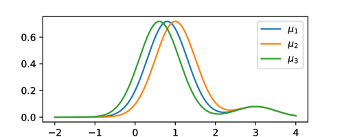
Figure 3: Reward distributions for arms in Settings 4 and 5.

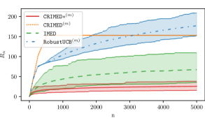
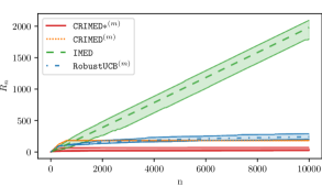
Figure 4: Cumulative regret for $100$ repetitions on Settings 4 (left) and 5 (right). Solid lines represent the means and shaded area are $90\%$ percentile intervals.

References

- Abbasi-Yadkori et al. (2018) Yasin Abbasi-Yadkori, Peter Bartlett, Victor Gabillon, Alan Malek, and Michal Valko. Best of both worlds: Stochastic & adversarial best-arm identification. In Conference on Learning Theory, pages 918–949. PMLR, 2018.
- Abernethy and Rakhlin (2009) Jacob Abernethy and Alexander Rakhlin. Beating the adaptive bandit with high probability. In 2009 Information Theory and Applications Workshop, pages 280–289. IEEE, 2009.
- Adams et al. (2019) John Adams, Darren Hayunga, Sattar Mansi, David Reeb, and Vincenzo Verardi. Identifying and treating outliers in finance. Financial Management, 48(2):345–384, 2019.
- Agrawal and Goyal (2012) Shipra Agrawal and Navin Goyal. Analysis of thompson sampling for the multi-armed bandit problem. In Conference on learning theory, pages 39–1. JMLR Workshop and Conference Proceedings, 2012.
- Agrawal and Goyal (2017) Shipra Agrawal and Navin Goyal. Near-optimal regret bounds for thompson sampling. Journal of the ACM (JACM), 64(5):1–24, 2017.
- Agrawal (2023) Shubhada Agrawal. Bandits with Heavy Tails: Algorithms Analysis and Optimality. PhD thesis, Tata Institute of Fundamental Research, 2023.
- Agrawal et al. (2020) Shubhada Agrawal, Sandeep Juneja, and Peter Glynn. Optimal -correct best-arm selection for heavy-tailed distributions. In Algorithmic Learning Theory, pages 61–110. PMLR, 2020.
- Agrawal et al. (2021) Shubhada Agrawal, Sandeep K Juneja, and Wouter M Koolen. Regret minimization in heavy-tailed bandits. In Conference on Learning Theory, pages 26–62. PMLR, 2021.
- Altschuler et al. (2019) Jason Altschuler, Victor-Emmanuel Brunel, and Alan Malek. Best arm identification for contaminated bandits. Journal of Machine Learning Research, 20(91):1–39, 2019.
- Audibert et al. (2009) Jean-Yves Audibert, Sébastien Bubeck, et al. Minimax policies for adversarial and stochastic bandits. In COLT, volume 7, pages 1–122, 2009.
- Auer et al. (1995) Peter Auer, Nicolo Cesa-Bianchi, Yoav Freund, and Robert E Schapire. Gambling in a rigged casino: The adversarial multi-armed bandit problem. In Proceedings of IEEE 36th annual foundations of computer science, pages 322–331. IEEE, 1995.
- Auer et al. (2002a) Peter Auer, Nicolo Cesa-Bianchi, and Paul Fischer. Finite-time analysis of the multiarmed bandit problem. Machine learning, 47(2-3):235–256, 2002a.
- Auer et al. (2002b) Peter Auer, Nicolo Cesa-Bianchi, Yoav Freund, and Robert E Schapire. The nonstochastic multiarmed bandit problem. SIAM journal on computing, 32(1):48–77, 2002b.
- Azize and Basu (2023) Achraf Azize and Debabrota Basu. Interactive and concentrated differential privacy for bandits. arXiv:2309.00557, 2023.
- Basu et al. (2022) Debabrota Basu, Odalric-Ambrym Maillard, and Timothée Mathieu. Bandits corrupted by nature: Lower bounds on regret and robust optimistic algorithm. arXiv:2203.03186, 2022.
- Bourel et al. (2020) Hippolyte Bourel, Odalric Maillard, and Mohammad Sadegh Talebi. Tightening exploration in upper confidence reinforcement learning. In International Conference on Machine Learning, pages 1056–1066. PMLR, 2020.
- Bubeck and Slivkins (2012) Sébastien Bubeck and Aleksandrs Slivkins. The best of both worlds: Stochastic and adversarial bandits. In Conference on Learning Theory, pages 42–1. JMLR Workshop and Conference Proceedings, 2012.
- Burnetas and Katehakis (1996) Apostolos N Burnetas and Michael N Katehakis. Optimal adaptive policies for sequential allocation problems. Advances in Applied Mathematics, 17(2):122–142, 1996.
- Cappé et al. (2013) Olivier Cappé, Aurélien Garivier, Odalric-Ambrym Maillard, Rémi Munos, and Gilles Stoltz. Kullback-leibler upper confidence bounds for optimal sequential allocation. The Annals of Statistics, pages 1516–1541, 2013.
- Catoni (2012) Olivier Catoni. Challenging the empirical mean and empirical variance: A deviation study. Ann. Inst. H. Poincaré Probab. Statist., 48(4):1148–1185, 11 2012.
- Charikar et al. (2017) Moses Charikar, Jacob Steinhardt, and Gregory Valiant. Learning from untrusted data. In Proceedings of the 49th Annual ACM SIGACT Symposium on Theory of Computing, pages 47–60, 2017.
- Chen et al. (2018) Mengjie Chen, Chao Gao, Zhao Ren, et al. Robust covariance and scatter matrix estimation under huber’s contamination model. The Annals of Statistics, 46(5):1932–1960, 2018.
- Devroye et al. (2016) Luc Devroye, Matthieu Lerasle, Gabor Lugosi, and Roberto I. Oliveira. Sub-gaussian mean estimators. The Annals of Statistics, 44(6):2695–2725, 2016. ISSN 0090-5364.
- Diakonikolas et al. (2018) Ilias Diakonikolas, Gautam Kamath, Daniel M Kane, Jerry Li, Ankur Moitra, and Alistair Stewart. Robustly learning a gaussian: Getting optimal error, efficiently. In Proceedings of the Twenty-Ninth Annual ACM-SIAM Symposium on Discrete Algorithms, pages 2683–2702. SIAM, 2018.
- Even-Dar et al. (2006) Eyal Even-Dar, Shie Mannor, Yishay Mansour, and Sridhar Mahadevan. Action elimination and stopping conditions for the multi-armed bandit and reinforcement learning problems. Journal of machine learning research, 7(6), 2006.
- Foster et al. (2020) Dylan J Foster, Claudio Gentile, Mehryar Mohri, and Julian Zimmert. Adapting to misspecification in contextual bandits. Advances in Neural Information Processing Systems, 33:11478–11489, 2020.
- Gajane et al. (2018) Pratik Gajane, Tanguy Urvoy, and Emilie Kaufmann. Corrupt bandits for preserving local privacy. In Algorithmic Learning Theory, pages 387–412. PMLR, 2018.
- Garivier et al. (2019) Aurélien Garivier, Pierre Ménard, and Gilles Stoltz. Explore first, exploit next: The true shape of regret in bandit problems. Mathematics of Operations Research, 44(2):377–399, 2019.
- Ghosh et al. (2017) Avishek Ghosh, Sayak Ray Chowdhury, and Aditya Gopalan. Misspecified linear bandits. In Proceedings of the AAAI Conference on Artificial Intelligence, volume 31, 2017.
- Golrezaei et al. (2021) Negin Golrezaei, Vahideh Manshadi, Jon Schneider, and Shreyas Sekar. Learning product rankings robust to fake users. In Proceedings of the 22nd ACM Conference on Economics and Computation, pages 560–561, 2021.
- Gupta et al. (2019) Anupam Gupta, Tomer Koren, and Kunal Talwar. Better algorithms for stochastic bandits with adversarial corruptions. In Conference on Learning Theory, pages 1562–1578. PMLR, 2019.
- Hampel et al. (1986) Frank R. Hampel, Elvezio M. Ronchetti, Peter J. Rousseeuw, and Werner A. Stahel. Robust Statistics: The Approach Based on Influence Functions. Wiley Series in Probability and Statistics. Wiley, 1st edition edition, January 1986. ISBN 0471829218. missing.
- Honda and Takemura (2009) Junya Honda and Akimichi Takemura. An asymptotically optimal policy for finite support models in the multiarmed bandit problem. arXiv:0905.2776, 2009.
- Honda and Takemura (2010) Junya Honda and Akimichi Takemura. An asymptotically optimal bandit algorithm for bounded support models. In COLT, pages 67–79. Citeseer, 2010.
- Honda and Takemura (2015) Junya Honda and Akimichi Takemura. Non-asymptotic analysis of a new bandit algorithm for semi-bounded rewards. Journal of Machine Learning Research, 16(113):3721–3756, 2015.
- Huber (1964) Peter J. Huber. Robust estimation of a location parameter. Ann. Math. Statist., 35(1):73–101, 03 1964. ISSN 0003-4851.
- Huber (1965) Peter J. Huber. A Robust Version of the Probability Ratio Test. The Annals of Mathematical Statistics, 36(6):1753 – 1758, 1965. URL https://doi.org/10.1214/aoms/1177699803.
- Huber and Ronchetti (2009) Peter J Huber and Elvezio M Ronchetti. Robust statistics; 2nd ed. Wiley Series in Probability and Statistics. Wiley, Hoboken, NJ, 2009. URL https://cds.cern.ch/record/1254106.
- Jun et al. (2018) Kwang-Sung Jun, Lihong Li, Yuzhe Ma, and Jerry Zhu. Adversarial attacks on stochastic bandits. Advances in Neural Information Processing Systems, 31, 2018.
- Kapoor et al. (2019) Sayash Kapoor, Kumar Kshitij Patel, and Purushottam Kar. Corruption-tolerant bandit learning. Machine Learning, 108(4):687–715, 2019.
- Kaufmann et al. (2012) Emilie Kaufmann, Nathaniel Korda, and Rémi Munos. Thompson sampling: An asymptotically optimal finite-time analysis. In Algorithmic Learning Theory: 23rd International Conference, ALT 2012, Lyon, France, October 29-31, 2012. Proceedings 23, pages 199–213. Springer, 2012.
- Kaufmann et al. (2016) Emilie Kaufmann, Olivier Cappé, and Aurélien Garivier. On the complexity of best-arm identification in multi-armed bandit models. The Journal of Machine Learning Research, 17(1):1–42, 2016.
- Lai and Robbins (1985) Tze Leung Lai and Herbert Robbins. Asymptotically efficient adaptive allocation rules. Advances in applied mathematics, 6(1):4–22, 1985.
- Lattimore and Szepesvári (2020) Tor Lattimore and Csaba Szepesvári. Bandit algorithms. Cambridge University Press, 2020.
- Liu and Shroff (2019) Fang Liu and Ness Shroff. Data poisoning attacks on stochastic bandits. In International Conference on Machine Learning, pages 4042–4050. PMLR, 2019.
- Lugosi and Mendelson (2019) Gábor Lugosi and Shahar Mendelson. Mean estimation and regression under heavy-tailed distributions: A survey. Foundations of Computational Mathematics, 19(5):1145–1190, 2019.
- Lykouris et al. (2018) Thodoris Lykouris, Vahab Mirrokni, and Renato Paes Leme. Stochastic bandits robust to adversarial corruptions. In Proceedings of the 50th Annual ACM SIGACT Symposium on Theory of Computing, pages 114–122, 2018.
- Mukherjee et al. (2021) Arpan Mukherjee, Ali Tajer, Pin-Yu Chen, and Payel Das. Mean-based best arm identification in stochastic bandits under reward contamination. Advances in Neural Information Processing Systems, 34:9651–9662, 2021.
- Neu (2015) Gergely Neu. Explore no more: Improved high-probability regret bounds for non-stochastic bandits. Advances in Neural Information Processing Systems, 28, 2015.
- Nikolakakis et al. (2021) Konstantinos E Nikolakakis, Dionysios S Kalogerias, Or Sheffet, and Anand D Sarwate. Quantile multi-armed bandits: Optimal best-arm identification and a differentially private scheme. IEEE Journal on Selected Areas in Information Theory, 2(2):534–548, 2021.
- Pogodin and Lattimore (2020) Roman Pogodin and Tor Lattimore. On first-order bounds, variance and gap-dependent bounds for adversarial bandits. In Uncertainty in Artificial Intelligence, pages 894–904. PMLR, 2020.
- Robbins (1952) Herbert Robbins. Some aspects of the sequential design of experiments. 1952.
- Seldin and Lugosi (2017) Yevgeny Seldin and Gábor Lugosi. An improved parametrization and analysis of the exp3++ algorithm for stochastic and adversarial bandits. In Conference on Learning Theory, pages 1743–1759. PMLR, 2017.
- Seldin and Slivkins (2014) Yevgeny Seldin and Aleksandrs Slivkins. One practical algorithm for both stochastic and adversarial bandits. In International Conference on Machine Learning, pages 1287–1295. PMLR, 2014.
- Thabane et al. (2013) Lehana Thabane, Lawrence Mbuagbaw, Shiyuan Zhang, Zainab Samaan, Maura Marcucci, Chenglin Ye, Marroon Thabane, Lora Giangregorio, Brittany Dennis, Daisy Kosa, et al. A tutorial on sensitivity analyses in clinical trials: the what, why, when and how. BMC medical research methodology, 13(1):1–12, 2013.
- Thompson (1933) William R Thompson. On the likelihood that one unknown probability exceeds another in view of the evidence of two samples. Biometrika, 25(3-4):285–294, 1933.
- Virtanen et al. (2020) Pauli Virtanen, Ralf Gommers, Travis E. Oliphant, Matt Haberland, Tyler Reddy, David Cournapeau, Evgeni Burovski, Pearu Peterson, Warren Weckesser, Jonathan Bright, Stéfan J. van der Walt, Matthew Brett, Joshua Wilson, K. Jarrod Millman, Nikolay Mayorov, Andrew R. J. Nelson, Eric Jones, Robert Kern, Eric Larson, C J Carey, İlhan Polat, Yu Feng, Eric W. Moore, Jake VanderPlas, Denis Laxalde, Josef Perktold, Robert Cimrman, Ian Henriksen, E. A. Quintero, Charles R. Harris, Anne M. Archibald, Antônio H. Ribeiro, Fabian Pedregosa, Paul van Mulbregt, and SciPy 1.0 Contributors. SciPy 1.0: Fundamental Algorithms for Scientific Computing in Python. Nature Methods, 17:261–272, 2020.
- Wang and Ramdas (2023) Hongjian Wang and Aaditya Ramdas. Huber-robust confidence sequences. arXiv:2301.09573, 2023.
- Xu et al. (2021) Yinglun Xu, Bhuvesh Kumar, and Jacob D Abernethy. Observation-free attacks on stochastic bandits. Advances in Neural Information Processing Systems, 34:22550–22561, 2021.
- Zimmert and Seldin (2019) Julian Zimmert and Yevgeny Seldin. An optimal algorithm for stochastic and adversarial bandits. In The 22nd International Conference on Artificial Intelligence and Statistics, pages 467–475. PMLR, 2019.