1-arcsecond imaging strategy for the LoTSS survey using the International LOFAR Telescope

We present the first wide area ($2.5\times 2.5$ $\mathrm{deg}^{2}$), deep (median noise of $\approx 80\mu\mathrm{Jy}{\mathrm{beam}}^{--1}$) LOFAR High Band Antenna image at a resolution of $1.2\arcsec\times 2\arcsec$. It was made from an 8-hour International LOFAR Telescope (ILT) observation of the ELAIS-N1 field at frequencies ranging from 120 to 168 MHz with the most up-to-date ILT imaging strategy. This intermediate resolution falls between the highest possible resolution (0.3″) achievable by using all International LOFAR Telescope (ILT) baselines and the standard 6-arcsecond resolution in the LoTSS (LOFAR Two-meter Sky Survey) image products utilising the LOFAR Dutch baselines only. This is the first demonstration of the feasibility of $\sim$1″imaging using the ILT, which provides unique information on source morphology at scales that fall below the surface brightness limits of higher resolutions. The total calibration and imaging time is approximately 52,000 core hours, nearly 5 times more than producing a 6″image. We also present a radio source catalogue containing 2263 sources detected over the $2.5\times 2.5$ $\mathrm{deg}^{2}$ image of the ELAIS-N1 field, with a peak intensity threshold of $5.5\sigma$. The catalogue has been cross-matched with the LoTSS deep ELAIS-N1 field radio catalogue, and its flux density and positional accuracy have been investigated and corrected accordingly. We find that $\sim$80% of sources which we expect to be detectable based on their peak brightness in the LoTSS 6″are detected in this image, which is approximately a factor of two higher than for 0.3″imaging in the Lockman Hole, implying there is a wealth of information on these intermediate scales.

1 Introduction

The LOw Frequency ARray (LOFAR; van Haarlem et al. (2013)) is a low-frequency radio interferometer operating below 250 MHz, with Low Band Antennas (LBAs) and High Band Antennas (HBAs) optimized for 10-80 MHz and 120-240 MHz respectively. Utilising the HBAs, the ongoing LOFAR Two-metre Sky Survey (LoTSS; Shimwell et al. (2017)) has published two data releases (Shimwell et al. 2019, 2022) with image products at a resolution of 6″. With long intra-continental baselines up to 2000 km, the International LOFAR Telescope (ILT) gives the potential to survey wide fields at an angular resolution of a few tenths of an arcsecond using the HBAs. This has been successfully demonstrated by Sweijen et al. (2022) with the development of ILT calibration strategies. A 7.4 $\mathrm{deg}^{2}$ image of the Lockman Hole at 144 MHz was produced, and its angular resolution is substantially increased from 6″ to 0.3″.

Currently, over 90% of the LoTSS has recorded the international baseline data. While processing individual sources in the field of view is computationally inexpensive (Morabito et al. 2022a), producing a multi-degree-scale field of view at sub-arcsecond resolution is estimated to take 250,000 core hours (Sweijen et al. 2022). While developments are being made to reduce this cost, it remains a significant challenge for the capacity of existing computing facilities, particularly when batch image processing is required for survey purposes. This challenge is amplified by the fact that LoTSS alone comprises 3168 pointings, and more pointings would be necessary for a $0.3\arcsec$ survey due to the decreased field of view. Making ILT images at an angular resolution around $\sim$1″, a resolution between 0.3″and 6″, balances amongst feasibility, scientific impact, affordable computing facilities and time. This was the first time that a well-calibrated $\sim$1″degree-scale field of view has been produced at low frequencies.

Imaging at this intermediate resolution would provide unique information on source morphology. As Sweijen et al. (2022) showed, only 40% of the compact sources detected at 6 arcsec resolution remain visible at 0.3 arcsec resolution. Therefore, a significant fraction of sources has extended emission on scales between 0.3″and 6″, indicating the need for intermediate-resolution imaging to study the nature of these objects. In other words, as the resolution decreases from $0.3\arcsec$ to $\sim$1″, the surface brightness sensitivity increases, allowing for the detection of extended emissions that would otherwise be too diffuse to be detected in the sub-arcsecond image. It will advance the detailed study of these sources, possibly dominated by star-forming galaxies whose emissions are on a scale of $\sim$1″, thereby enhancing our knowledge of research topics such as star formation and active galactic nuclei (AGN). In terms of the computational cost, the full process of calibrating and making a $1.2\arcsec\times 2\arcsec$ image from an 8-hour LoTSS observation takes approximately 52,000 core hours, which is nearly 5 times less compared to the sub-arcsecond imaging. On account of this, producing $\sim$1″images as the standard image products for LoTSS-like ILT surveys is feasible without a major computing infrastructure update and will help drive forward extragalactic science.

The ELAIS-N1 field is originally one of a few fields covered by the European Large Area Infrared Space Observatory Survey (ELAIS) (Oliver et al. 2000) in the infrared. Multi-wavelength observations have been conducted since, making ELAIS-N1 field one of the most observed extragalactic degree-scale fields. At radio wavelengths, the ELAIS-N1 field has been covered in multiple large-area radio surveys in a frequency range from 38 MHz to 4.85 GHz. Some of these surveys at lower frequencies include the Cambridge Survey of Radio Sources catalogue at 151 MHz (6C; Hales et al. 1990) and at 38 MHz (8C; Hales et al. 1995), the Very Large Array (VLA) Low-frequency Sky Survey (VLSS) at 74 MHz (Cohen et al. 2007), the all-sky TIFR GMRT Sky Survey (TGSS) by the Giant Metrewave Radio Telescope (GMRT) at 150 MHz (Intema et al. 2017) and the Westerbork Northern Sky Survey (WENSS) at 325 MHz (Rengelink et al. 1997). There have also been radio surveys specifically targeting the ELAIS-N1 field, a comparison among those in terms of the area covered, root mean square (RMS) noise and frequency are presented (see Sabater et al. 2021, Figure 1). For recent low-frequency observations that target the ELAIS-N1 field, the Giant Metrewave Radio Telescope (GMRT) has conducted at least four observations on the ELAIS-N1 field (Garn et al. 2008; Sirothia et al. 2009; Taylor & Jagannathan 2016; Ocran et al. 2020) at frequencies of 325 MHz and/or 610 MHz. However, none of these low-frequency observations achieved a resolution better than 5″. As one of the four LoTSS Deep Fields (Best et al. 2023), the ELAIS-N1 field was imaged at a resolution of 6″, covering $\sim$68 $\mathrm{deg}^{2}$ (Sabater et al. 2021). It achieves a root mean square noise level of $\sim$19$\,\mu\mathrm{Jy}\ {\mathrm{beam}}^{-1}$ in the central region at a central frequency of 144 MHz. This depth is accomplished by amalgamating observations over $\sim$200 hours instead of a standard 8-hour observation. A corresponding radio catalogue has also been presented. Kondapally et al. (2021) compiled a multi-wavelength catalogue where multi-wavelength counterparts of radio sources are identified. In this work, we make use of this existing optically cross-matched radio catalogue to cross-check the radio catalogue obtained from our 1.2″image.

In this paper, we have tested and further improved the ILT calibration and imaging strategy following the pilot ILT sub-arcsecond imaging case (Sweijen et al. 2022). We present a deep (median noise of $\approx$80 $\mu\mathrm{Jy}{\mathrm{beam}}^{-1}$), $2.5\times 2.5$ $\mathrm{deg}^{2}$ image of the ELAIS-N1 field at a resolution of $1.2\arcsec\times 2\arcsec$ , and provide its catalogue after careful cross-matching with existing catalogues at radio wavelengths. The most up-to-date workflow for making such intermediate-resolution images is outlined. This paper is organised as follows. Section 2 describes the 8-hour ILT observation of the ELAIS-N1 field used in this work. In Section 3, we present the data reduction procedures and the image produced, with a special focus on selecting suitable calibrators within the field to correct for the direction-dependent effects (DDEs). In Section 4, after the quality examination of the catalogue produced in terms of the flux density scale and positional offsets, the final image and catalogue are presented after correction. Section 5 presents a detailed discussion of its scientific impact and computational cost. Finally, Section 6 summarises and concludes the work.

2 Observations

On 26 November 2018, the ELAIS-N1 field was observed using LOFAR’s HBAs for a total of 8 hours at frequencies ranging from 120 to 168 MHz. 3C 295 was observed prior to the observation for 10 minutes as the primary calibrator. An overview of the observation parameters is given in Table 1. This observation used 51 stations including 24 Dutch core stations, 14 remote stations and 13 international stations, resulting in a maximum baseline of 1514 km. The observation was taken in HBA dual inner mode where only the inner 24 tiles of the 48 in the remote stations are used in order to mimic the core stations. However, the full 96 tiles in each ILT station are used. Figure 1 plots the $uv$-coverage of this observation, only one in ten $uv$ points in time and one in 40 $uv$ points in frequency are plotted. There are fewer baselines in the range between 80 to 180 km, due to a scarcity of stations between the Dutch and German HBA locations.

Table 1: International LOFAR telescope HBA observation parameters

Observation IDs	L686956 (3C295) L686962 (ELAIS-N1)
Pointing centres	$16^{h}11^{m}00^{s}$+$54^{d}57^{m}00^{s}$ (ELAIS-N1) $14^{h}11^{m}20.4^{s}+52^{d}12^{m}10.08^{s}$ (3C295)
Observation date	2018 Nov 26
Total on-source time	10 min (3C295) 8h (ELAIS-N1)
Correlations	XX, XY, YX, YY
Sampling mode	8 bit
Sampling clock frequency	200 MHz
Frequency range	120-187 MHz
Used frequency range	120-168 MHz
Used bandwidth	48 MHz (ELAIS-N1,3C295)
Bandwidth per SB	195.3125 kHz
Channels per SB	64
Stations	51 total 13 International 14 remote 24 core (48 split)

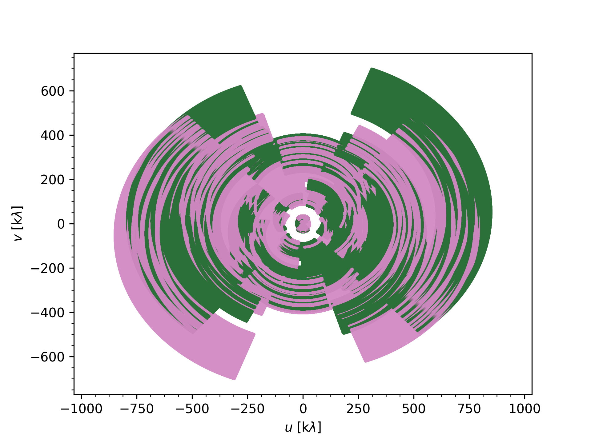
Figure 1: The $uv$-coverage for the ELAIS-N1 field observation at 120-168 MHz. The maximum baseline for this observation is 1514 km (or 853 $k\lambda$). To improve readability, only one in ten $uv$ points in time and one in 40 $uv$ points in frequency are plotted. The plot depicts symmetric $uv$ points due to conjugate visibilities, where the two colours represent these symmetric $uv$ points.

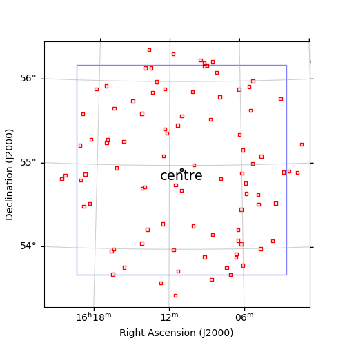
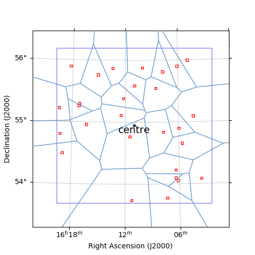
Figure 2: The boundary of the ELAIS-N1 field image made is defined by the outer blue square. The positions of direction-dependent calibrators are denoted by red small squares, while the pointing centre is marked by a blue solid dot. The left panel shows all self-calibration calibrator candidates, and the right panel displays the selected 28 calibrators. Each blue polygon in the right panel contains one calibrator, which is applied to correct the direction-dependent effects (DDEs) of the corresponding region.

3 Data Processing: calibration and imaging

The procedures for making the final calibrated and deconvolved $2.5\times 2.5$ $\mathrm{deg}^{2}$ image from our 8-hour ELAIS-N1 field observation can be divided into 4 major steps:

1. Calibration of all Dutch stations

2. Direction-independent calibration for international stations

3. Direction-dependent calibration for international stations

4. Making a $\sim$1″image from the calibrated data

The $2.1$ TB ILT data we began with has a time and frequency resolution of 2 seconds and $12.207\ \mathrm{kHz}$, respectively, referred to as the ’original data’ in this manuscript. However, it’s worth noting that the time resolution was initially averaged from 1 second to 2 seconds. For survey-related imaging reaching or exceeding the FWHM of the international station’s primary beam, we recommend using a 1-second time resolution to reduce the effects of time smearing.

3.1 Calibration of Dutch stations

We started the standard LOFAR HBA data reduction and calibration process using Prefactor (van Weeren et al. 2016; Williams et al. 2016; de Gasperin et al. 2019). This pipeline consists of two parts: a calibrator pipeline and a target pipeline. Target observations are bookended by short observations of a flux-density calibrator. The calibrator pipeline utilized these observations to rectify three significant systematic effects: the phase offsets between the X and Y polarisations, station bandpasses, and clock offsets between stations. These corrections were derived for all stations, including international ones. This was done using a $\sim$10$\mathrm{min}$ observation of 3C 295. Subsequently, the target pipeline applies these corrections, averages the data to an integration time of $8$ seconds and a frequency channel width of $48.828\ \mathrm{kHz}$, and removes the international stations. The Faraday rotation was then corrected first, using RMextract (Mevius 2018). Finally, a phase calibration was performed using the Tata Institute of Fundamental Research GMRT Sky Survey’s sky model (Intema et al. 2017). This gives a direction-independent bulk correction of the ionospheric corruptions for the Dutch stations.

Direction-dependent calibration to correct remaining DDEs across the field of view was subsequently performed with the ddf-pipeline (Shimwell et al. 2019; Tasse et al. 2021). This provided a high-quality 6″resolution model of the field that will be used for source subtraction in the next step.

3.2 Direction-independent Calibration of the international stations

The LOFAR-VLBI pipeline (Morabito et al. 2022a) was employed to conduct the direction-independent calibration of the international stations. This started with applying the solutions obtained by Prefactor to the original data. Next, bright and compact sources within the ELAIS-N1 field were selected, using the Long-Baseline Calibrator Survey (LBCS, Jackson et al. (2016, 2022), as candidate in-field calibrators for direction-independent calibration of the international stations. The in-field calibrator ILTJ160607.63+552135.5 was hand-picked from these LBCS candidates. The data was then phase-shifted to the in-field calibrator position, and all core station visibility data were phased up into a single superstation.

Self-calibration was used to calibrate the chosen in-field calibrator. As a starting model, a point-source model was used. After an initial round of phase-only calibration against the starting model, an updated model was created after each iteration. Three iterations of phase calibration were followed by 5 iterations of phase and amplitude calibration, for a total of eight iterations.

After that, the $6\arcsec$ model produced and described in 3.1 was subtracted outside of the international station’s central field of view ($2.5\times 2.5$ $\mathrm{deg}^{2}$). This was implemented to suppress interference from sources outside the target region during the imaging and calibration processes. This interference is intensified on Dutch stations due to their field of view being twice as large, leading to less primary beam suppression of distant sources compared to international stations.

As a final step, solutions derived from the self-calibration procedure described above on the in-field calibrator is applied to the data.

3.3 Direction-dependent calibration for international stations

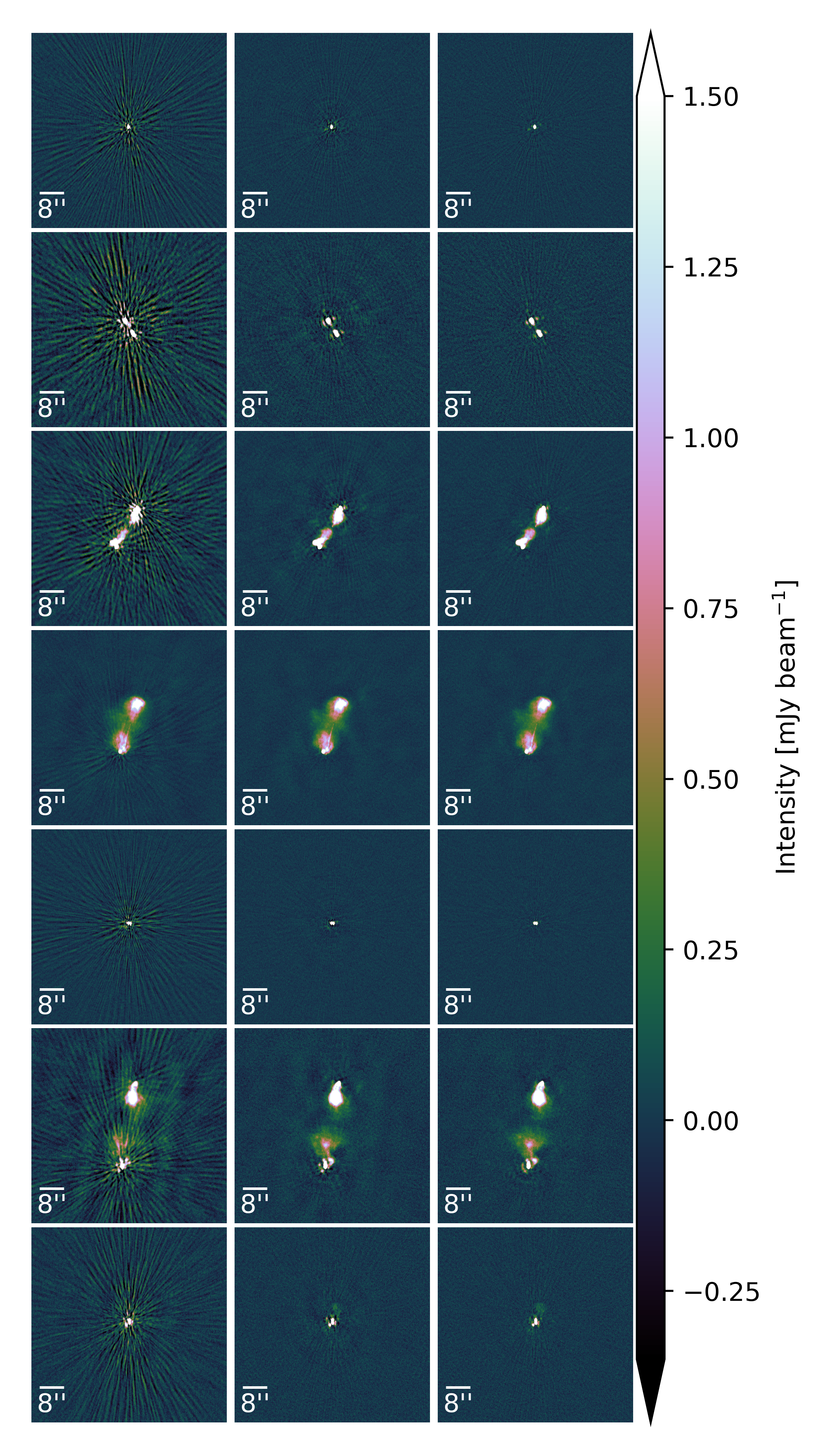
Figure 3: Each row of images showcases the iterative self-calibration process of one calibrator in correcting direction-dependent effects (DDEs). The three columns correspond to the calibrator’s images with 0, 2, and 4 iterations, representing no correction, dTEC-only correction, and dTEC and amplitude/phase correction, respectively. Each image has a size of $64\times 64$ arcsec and contains 1600 pixels by 1600 pixels.

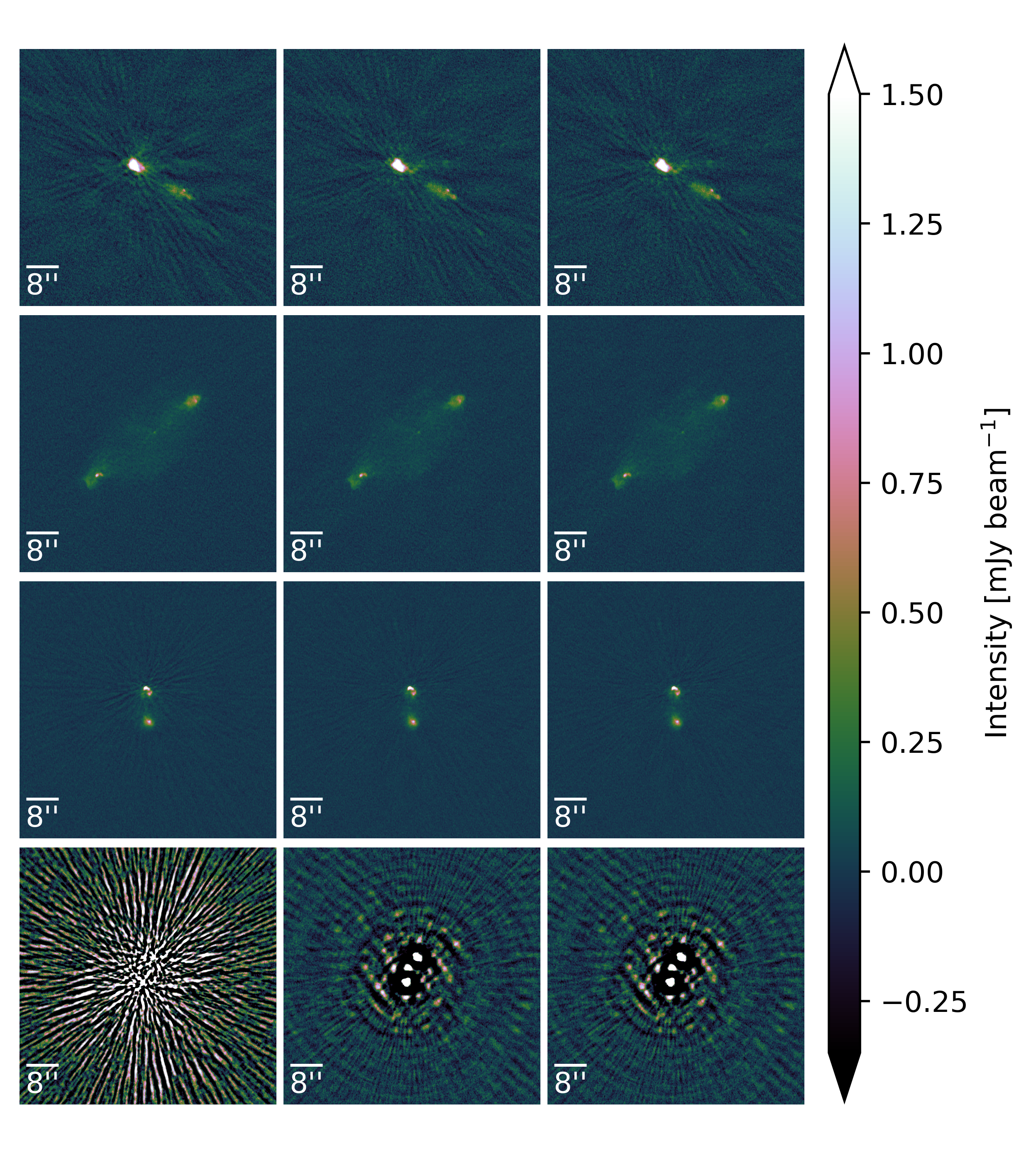
Figure 4: The self-calibration of the four calibrator candidates in which correcting direction-dependent effects (DDEs) was unsuccessful. The three columns show the four candidates’ images with 0, 4, and 8 iterations of self-calibration, representing no correction, dTEC-only correction, and dTEC and amplitude/phase correction, respectively. Each image has a size of $64\times 64$ arcsec and contains 1600 pixels by 1600 pixels.

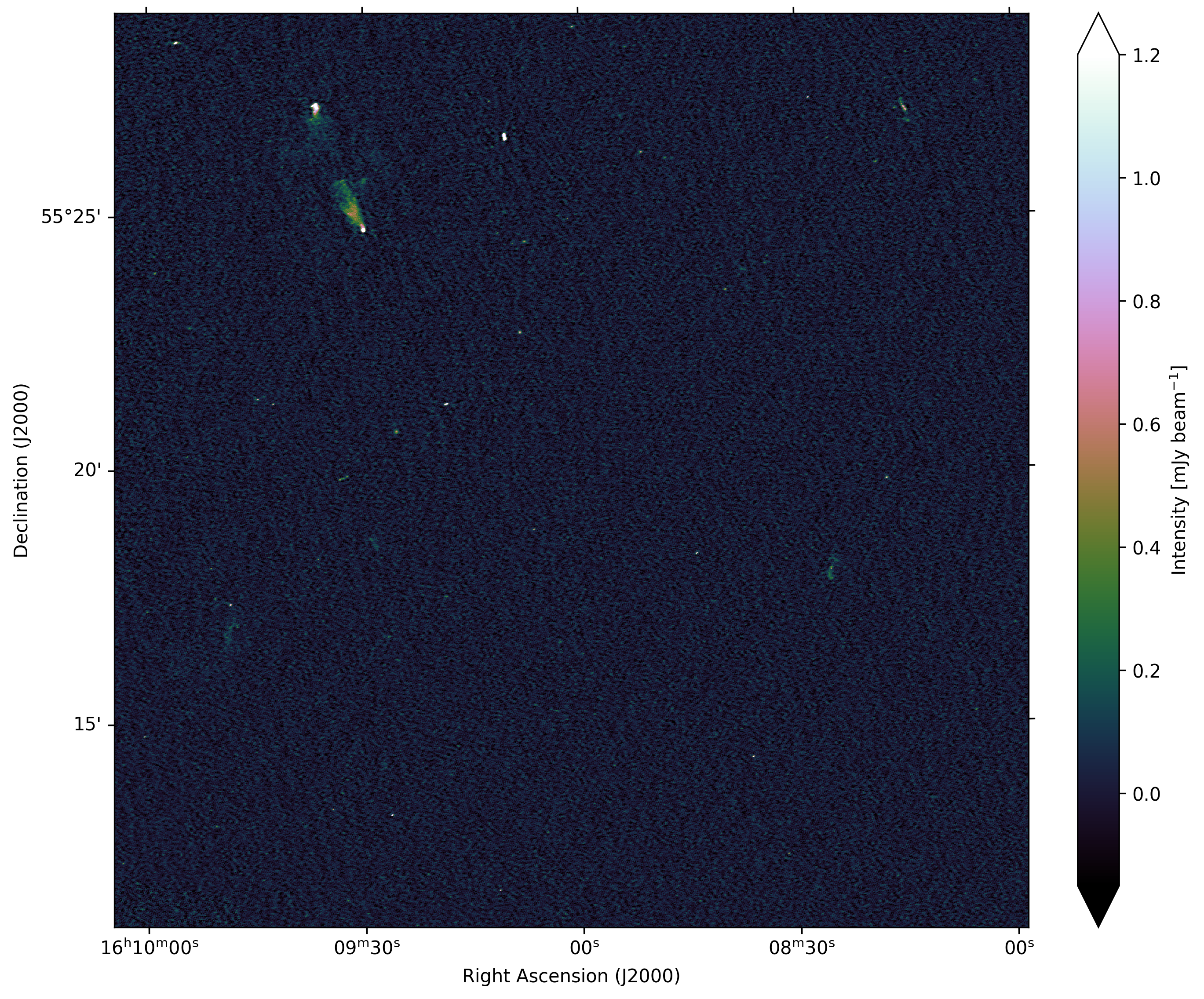
Figure 5: This zoom-in image depicts a central region in the ELAIS-N1 field, which was created using an 8-hour international LOFAR telescope observation at 120-168 MHz. This region is centred at ($16^{h}09^{m}01.36^{s}$, $55^{m}19^{m}56.7^{s}$) and is $0.3\mathrm{deg}\times 0.3\mathrm{deg}$ in size, with a resolution of $1.2\times 2$ ″. The colorbar represents the flux density from -$2\sigma$ to $20\sigma$, where $\sigma=0.122$ mJy beam^-1 is the approximate RMS noise in this region of the image.

In order to map the ELAIS-N1 field, it is imperative to mitigate the residual direction-dependent effects (DDEs), which are predominantly induced by the ionosphere. In accordance with the DDE calibration methodology outlined by Sweijen et al. (2022), we initially identified 93 potential DDE calibrators from the ELAIS-N1 LOFAR Deep field radio catalogue (Sabater et al. 2021). The selection criterion for these candidates was based on their peak intensities, which were required to be greater than $25$ mJy per beam. Subsequently, 93 distinct data sets were generated by phase-shifting and averaging, centred at each respective DDE calibrator. The left panel of Figure 2 illustrates the RA-DEC distribution of these DDE calibrator candidates.

For each of the 93 data sets, we undertook an iterative self-calibration procedure, as described by van Weeren et al. (2021) to correct for their total electron content (TEC) values of international stations. This was achieved through the facetselfcal.py Python script which employs the Default Preprocessing Pipeline (DPPP, van Diepen et al. (2018)) and WSCLEAN (Offringa et al. 2014; Offringa & Smirnov 2017). To be more specific, each self-calibration iteration generated a solution that was used to correct the differential TEC values of the dataset ($\sim$1 minutes), and optionally correct the phase and amplitude (i.e., complex gain) on longer timescales ($>20$ min) for candidates with a higher flux density to correct the inaccuracy in the LOFAR beam model. As a result of this procedure, we were able to identify and further select calibrators whose DDEs on the image plane could be effectively removed. We applied the solution obtained at each iteration to produce an image of size $64\times 64$ arcsec, with a pixel size of 0.04″. The images, centred on the respective calibrator candidates, were generated using WSCLEAN with a resolution of 0.3″, which is the full resolution for ILT. Figure 3 demonstrates the iterative DDE calibration process for seven calibrator candidates after completing the 0th, 2nd, and 4th iteration respectively, representing no correction, dTEC-only correction, and dTEC and amplitude/phase correction, respectively. The images in each column of the figure depict the gradual reduction of calibration artefacts resulting from DDEs after the completion of the 2nd and 4th self-calibration iterations.

For each of the 93 data sets, we selected a single solution from the multiple self-calibration solutions generated during iterative processes. This specific solution was chosen because it achieved the lowest noise level when applied to the phase-shifted visibility data centred at the position of this specific candidate, outperforming all other solutions. As an example, if the image produced with the 6th iterative solution demonstrated the lowest noise level among all available options, we would opt for it.

Not all self-calibration calibrator candidates yield self-calibration solutions that effectively correct for nearby DDEs. There are candidates that do not have enough flux density on the longer baselines to be successfully self-calibrated. Some candidates exhibit unaltered noise levels even after undergoing several iterations, while others have inadequate dynamic ranges (defined as the peak intensity divided by the RMS noise). Four examples are demonstrated in Figure 4, where the first, second, and fourth calibrator candidates result in a dynamic range of less than 20 after 8 rounds of calibration iterations, while the second candidate provided the lowest dynamic range of the three ($\sim$10). The third candidate illustrated in the figure achieved a good dynamic range of around 36 at Iteration 2; however, after that, the dynamic range dropped and converged at Iteration 4, with a noise level reduction of less than 8% compared to its 0th Iteration, when no calibration had been applied.

Given that it is not always possible to effectively remove the DDEs of every calibrator candidate, we developed specific selection criteria to identify calibrators that can effectively address DDEs, as follows:

1. During each iteration, the image of the selected calibrator must exhibit an increasing trend in the image dynamic range and a decreasing trend in noise level until convergence.

2. The minimum image dynamic range of the calibrator must exceed a threshold value. In our case, the threshold was set to $28$.

3. The application of self-calibration should result in a reduction percentage in noise level that exceeds a given threshold. In our study, the threshold was set to $8\%$ as compared to when no self-calibration was applied.

It is worth noting that the chosen threshold values of $28$ and $8\%$ were based on our experimental findings and may vary for different observations and calibrator sets. Further investigation is currently in progress to explore the potential variability of these thresholds. Furthermore, the minimum number of selected calibrators and their distribution requires further attention.

As a result, we selected 28 solutions from 28 calibrators. To further validate our selection, we visually inspected the images of each chosen calibrator to confirm that the DDE effects surrounding them had been effectively removed. In Figure 2, the right panel showcases the distribution of the selected DDE calibrators, marked by red boxes. The self-calibration solution chosen for each of these calibrators will be applied to their respective surrounding areas, marked by blue boundaries. No other self-calibration solutions were used during the final imaging process.

3.4 Imaging and results

We utilised the facet-imaging mode from WSCLEAN to generate a $2.5\times 2.5$ $\mathrm{deg}^{2}$ image of the ELAIS-N1 field, covering an area of 6.45 $\mathrm{deg}^{2}$ of field. To achieve this, we averaged the data to an integration time of 4 seconds and a frequency channel width of 48.828 kHz. We limited the $uv$ data to be larger than $80\lambda$. Our imaging process employed Briggs’ weighting (robust = $-1.5$), auto-masking, the multi-scale CLEAN deconvolution algorithm (Cornwell 2008; Offringa & Smirnov 2017), and WSCLEAN’s wide-field imaging module wgridder (Arras et al. 2021; Ye et al. 2022). The resulting image has a size of 22500 by 22500 pixels, with a pixel size of 0.4 arcsec and a taper size of 1.2 arcsec.

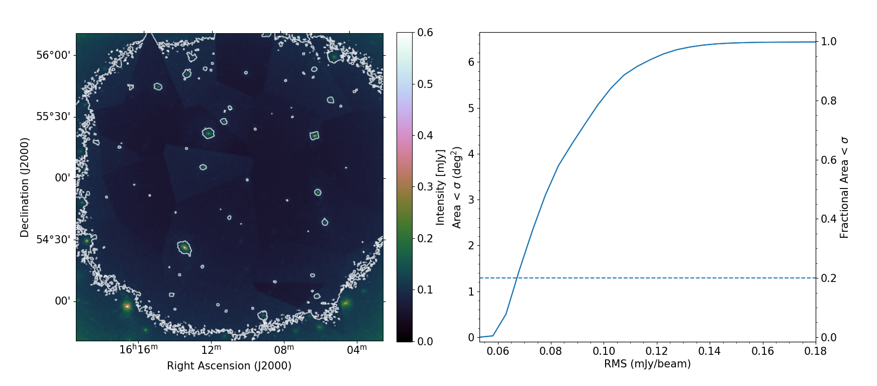
Figure 6: The left panel of this figure shows the contours of 0.1 mJy $\mathrm{beam}^{-1}$ overlaid on the RMS noise image of the ELAIS-N1 field, acquired at a resolution of 1.2 arcsec. The local RMS noise exhibits peaks at the positions of bright sources, indicating that their direction-dependent effects (DDEs) are not completely eliminated. The right panel depicts the cumulative ratio of pixels in the RMS image with intensity greater than the specified RMS noise value.

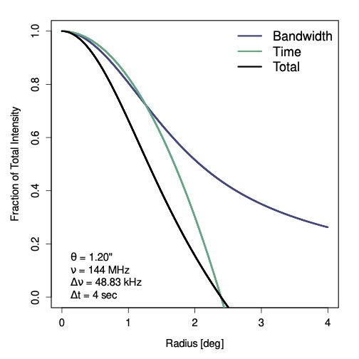
Figure 7: Effects of bandwidth and time smearing: changes in the fraction of initial total intensity for a point source as a function of its distance from the pointing centre. The calculation is based on Eqns. (18-43) and (18-24) of Bridle & Schwab (1999)

The final primary-beam-corrected image at $1.2\arcsec\times 2\arcsec$ resolution can be accessed online . Its positional offsets and flux scale have been corrected, and the procedures for these corrections will be discussed in Section 4. To illustrate the resolution, quality, and a range of sources in the field, Figure 5 displays a $0.3\times 0.3$ $\mathrm{deg}^{2}$ area of the final image, centred at ($16^{h}09^{m}01.36^{s}$, $55^{m}19^{m}56.7^{s}$), which is 28.5 arcminute from the image phase centre ($16^{h}11^{m}00^{s}$, $54^{m}57^{m}00^{s}$).

We also generated an RMS noise map from the flux- and astrometric-corrected image using the source finder package PyBDSF (Mohan & Rafferty 2015), with the parameters described in Section 4. The resulting RMS noise distribution is shown on the left side of Figure 6, with a contour plotted at 0.1 mJy ${\mathrm{beam}}^{--1}$. The contours surrounding some of the brightest sources suggest that their DDEs have not been completely removed. As seen in the right plot of Figure 6, the inner 20% of the image has a noise level below 0.068 mJy ${\mathrm{beam}}^{--1}$. In addition, some small facet-to-facet variations in the noise are visible to the varying quality of the DDE solutions.

Figure 7 provides information on the amount of bandwidth and time smearing when imaging at a resolution of 1.2 ″, with time and frequency resolution of 4 seconds and 48.83 kHz, respectively. We considered a compromise between the amount of smearing and imaging speed when selecting the averaging settings. For general reference, 20% losses occur at a radius of 0.74 degrees, while 50% losses occur at a radius of 1.30 degrees.

In Figure 8, we demonstrate three sources imaged at resolutions of 6″, 1.2″, and 0.3″respectively. These sources were selected from our catalog of 28 DDE calibrators. The 6″images were cutouts from the LOFAR ELAIS-N1 deep field image (Sabater et al. 2021), whereas the 0.3″images were obtained during the self-calibration procedure detailed in Section 3.3. Figure 8 reveals that these sources, which appeared compact in the 6″image, exhibit significant levels of resolved emission at higher resolutions. Consequently, the high-resolution images provide more intricate and informative details about the sources. We also selected 40 extended sources whose peak flux is larger than 20 mJy beam^-1 to display in the Appendix A.

›

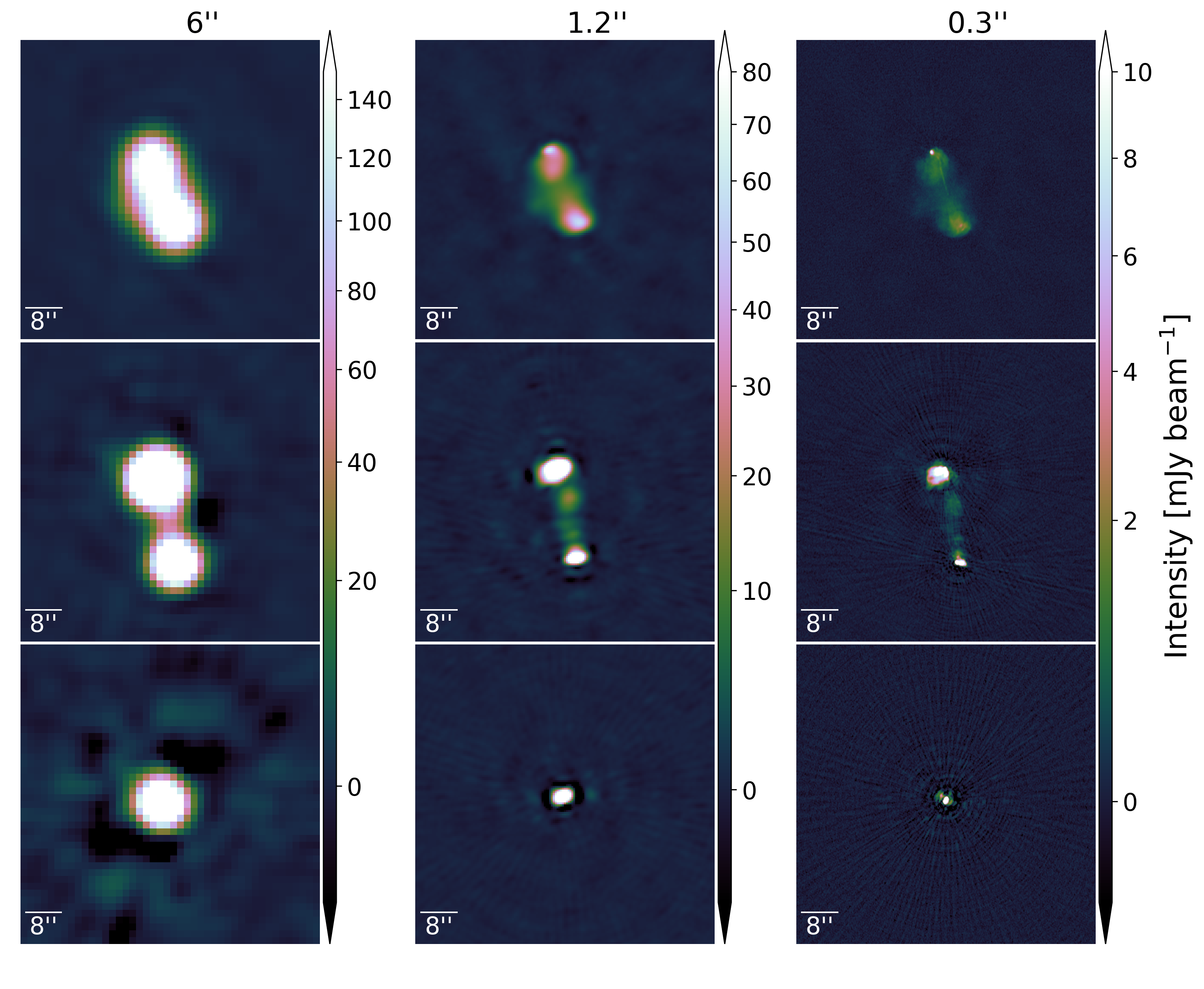
Figure 8: Three sources imaged at three different resolutions, namely 6″, 1.2″, and 0.3″. Left: cutouts extracted from the 6″LOFAR deep field image; centre: cutouts from our 1.2″image, which is presented in this paper; right: cutouts obtained from the 0.3″image created from our 8-hour ILT observation.

3.5 Computational Cost

It took $\sim$52,000 core hours to generate this $1.2\arcsec\times 2\arcsec$ image from the 8-hour LOFAR LoTSS observation data for the ELAIS-N1 field, which is nearly five times quicker than sub-arcsecond imaging (requiring $\sim$250,000 core hours (Sweijen et al. 2022)).

The approximate core hour distribution for this process includes $\sim$2,000 for calibrating all Dutch stations using Prefactor, $\sim$10,000 for direction-dependent calibration for Dutch stations with the ddf-pipeline, $\sim$7,000 performing direction-independent calibration for international stations, $\sim$10,000 for subtracting the 6″model, and another $\sim$10,000 for completing direction-dependent calibration for international stations.

Subsequent to these calibrations, the imaging step consumes $\sim$13,000 core hours of computational resources, and it is also one of the most memory-intensive steps. It takes around 6 days to produce the final 1.2″image from this fully-calibrated 8-hour LOFAR observation, which can run on a single compute node. The node used for imaging consisted of 512 GB RAM and dual 24-core Dual Intel Xeon Gold 5220R with hyper-threading. Hence, producing images with $\sim$1″resolution as a standard product for LoTSS-like ILT surveys can be accomplished without substantial upgrades to the current computing infrastructure.

4 Radio source catalogue

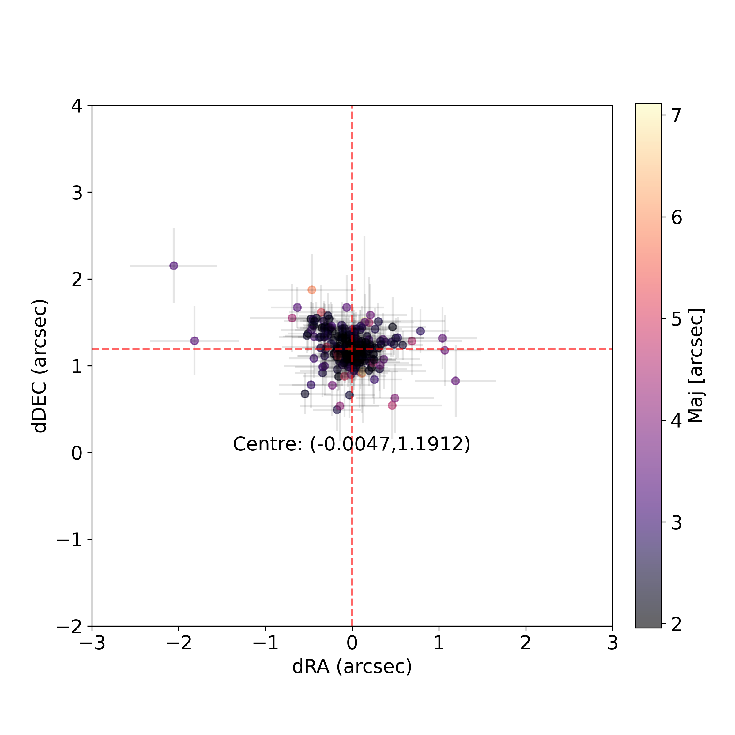
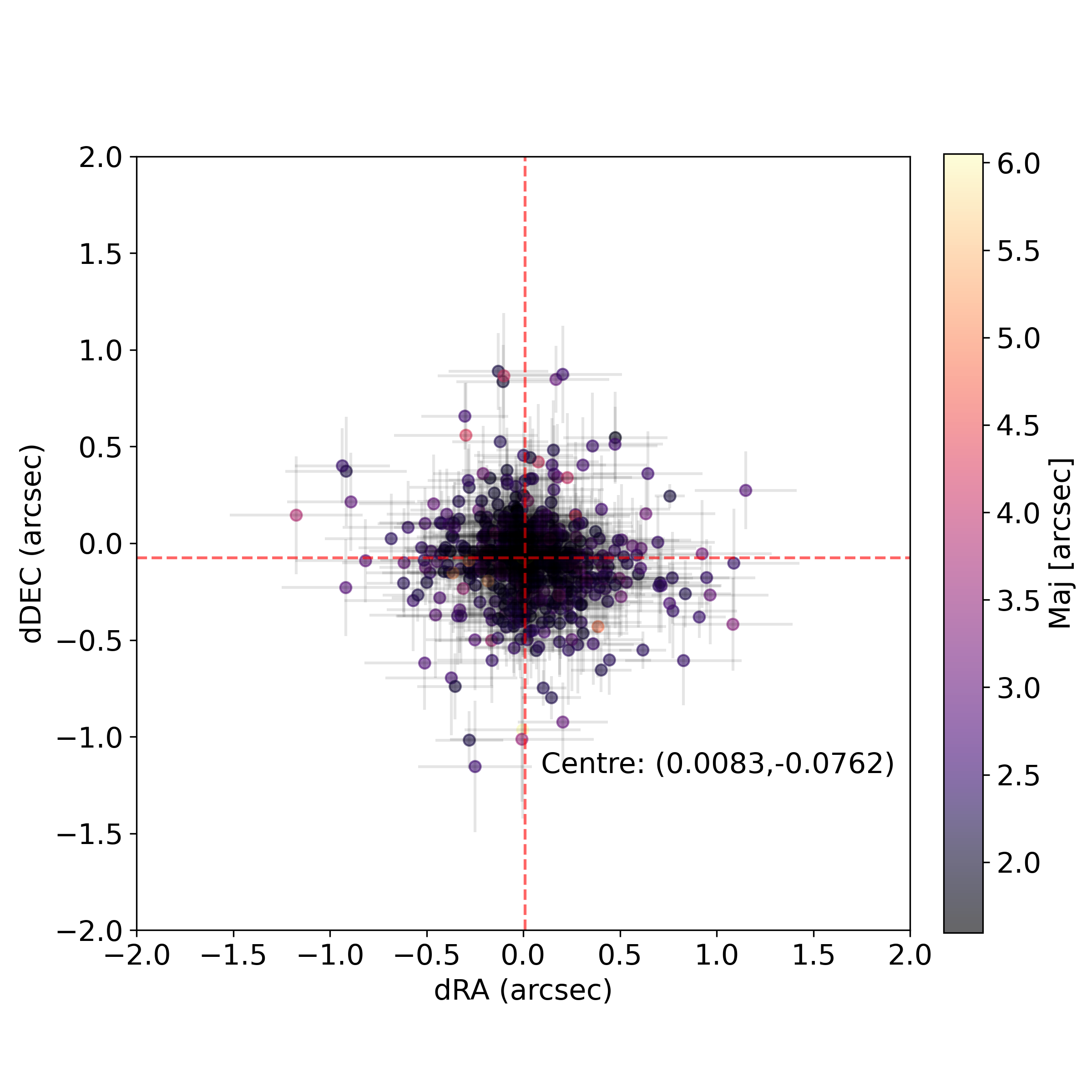
Figure 9: Left: Positional offsets of selected cross-matched sources between two catalogues, one is extracted from the 6″LOFAR deep image of the ELAIS-N1 field, and the other one is obtained from our current 1.2″image. The median values of the offset are $\mathrm{dRA}=-0.0047$″($\sigma=0.0939\arcsec$) and $\mathrm{dDEC}=1.1912\arcsec$ ($\sigma=0.0419$ ″). Right: Positional offsets of selected cross-matched sources from two catalogues, one is the optical catalogue of the ELAIS-N1 field, and the other one is our corrected radio catalogue. The median values of the offset are $\mathrm{dRA}$ = 0.0083″($\sigma$ = 0.0817″) and $\mathrm{dDEC}=-0.0762$ ($\sigma$ = 0.0605″). The near-to-zero median values validate the position offset correction. The error bar of each source is taken from the source extraction output of package PyBDSF.

To generate a preliminary radio source catalogue from our ELAIS-N1 image, we employed the source extraction package PyBDSF. The parameters used in PyBDSF were taken from the HBA deep fields settings (see Appendix C of Sabater et al. (2021)). In addition to generating the radio source catalogue, PyBDSF also generated an RMS noise map as displayed in the left panel of Figure 6, as well as fitted Gaussian and residual maps. The RMS noise map indicates a noticeable increase in noise level from the image’s centre to its edge due to the primary beam correction.

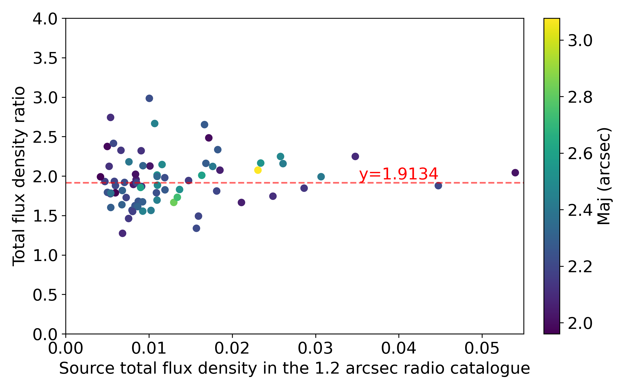
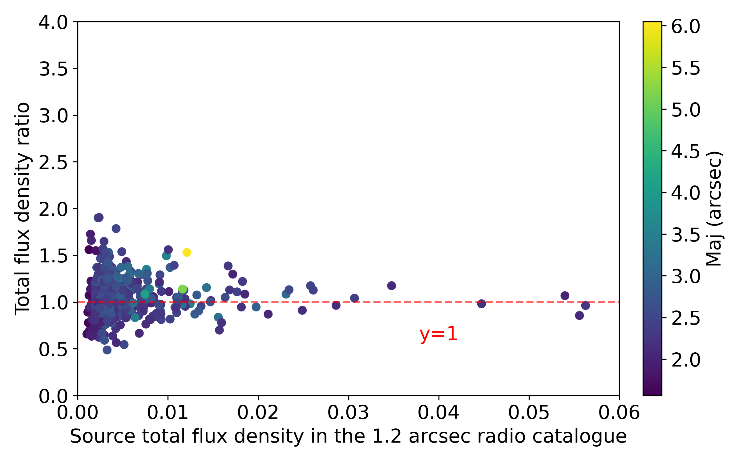
Figure 10: Left: The flux density ratio of 73 compact sources between our 1.2″catalogue and the 6″deep field catalogue is presented. The median value of 1.9134 is used as the flux scaling factor. Right: The flux scaling factor is applied to correct the flux densities of 503 compact sources in our 1.2 arcsec catalogue. As a result, the flux density ratios between the corrected flux densities and their corresponding values in the 6″deep field catalogue are observed to be scattered around 1.

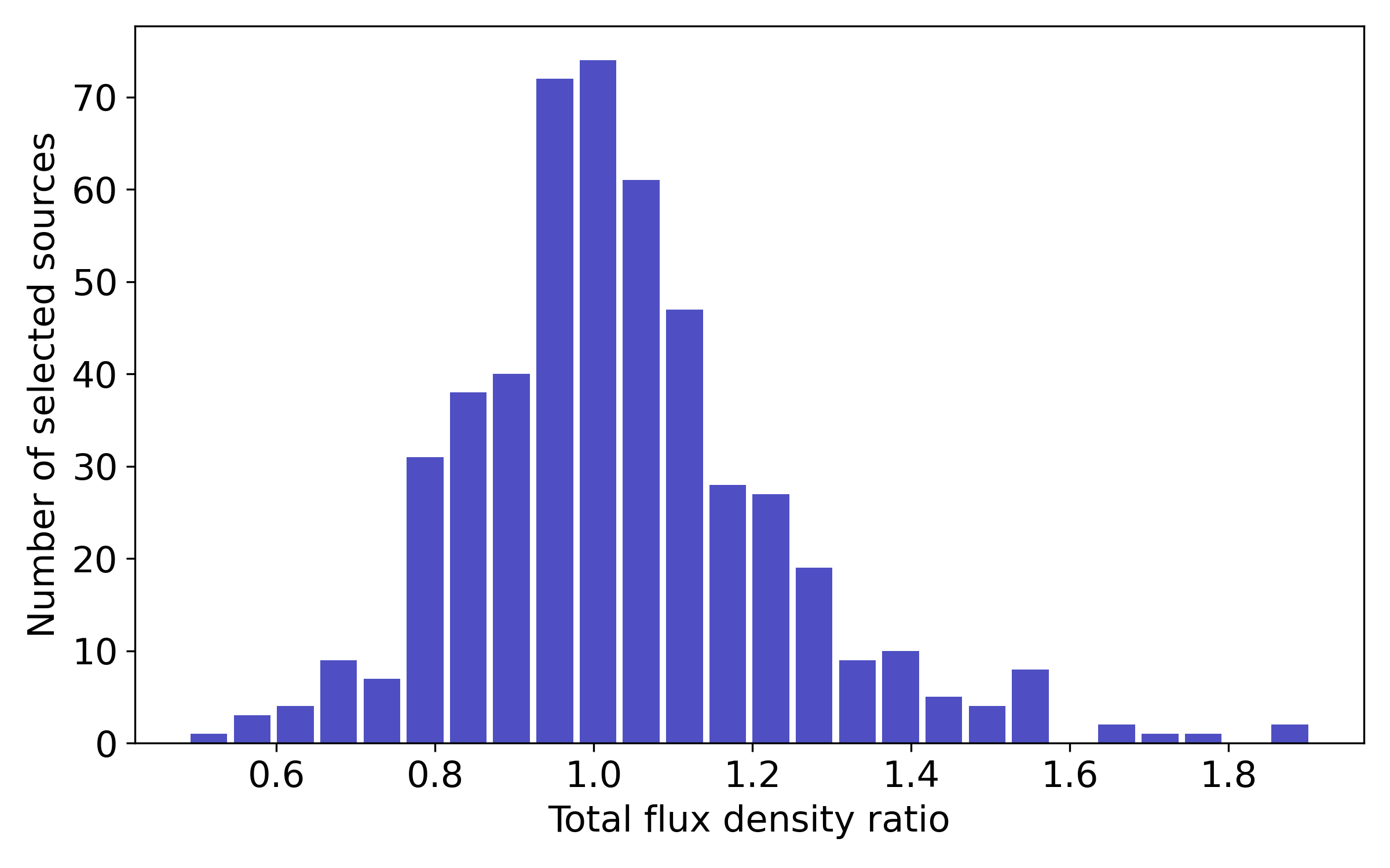
Figure 11: The histogram presents the flux density ratios of 503 selected compact sources, with the distribution observed to be centred around 1. This confirms the validity of the obtained scaling factor.

4.1 Astrometric precision

As the positions of our sources were extracted from our 1.2″ELAIS-N1 image, any phase calibration errors in making this image could result in source position offset. To address this issue, we cross-matched our 1.2″radio catalogue with the LOFAR 6″ELAIS-N1 deep field radio catalogue (Sabater et al. 2021) using TOPCAT (Taylor 2005), allowing for a maximum positional error of 6″. The 6″radio catalogue was extracted from the LOFAR 6 arcsec-resolution deep HBA image of the ELAIS-N1 field (Sabater et al. 2021), which has undergone examination through multi-wavelength source associations and cross-identifications with multiple optical observations (Kondapally et al. 2021), so it serves as a high-quality benchmark for our catalogue. As a result, 2 990 sources were cross-matched with the 6″ELAIS-N1 deep field radio catalogue.

Compact and bright sources tend to have more accurate positions because it is easier for the source extraction package to measure their positions with lower uncertainties, as opposed to extended or less bright sources. Subsequently, we selected 255 compact and bright sources to assess the astrometric accuracy of our image. In Figure 9, we illustrate the positional offsets in both right ascension (RA) and declination (DEC) for these 255 selected sources, which meet the criteria of having a flux density larger than 2 mJy and only one Gaussian component with an FWHM of the major axis smaller than 7.2 arcseconds (1.2 times the resolution of the 6″Deep image).

The right ascension offset, denoted as dRA on the $x$-axis, is defined as $\mathrm{dRA}=\mathrm{RA}_{\mathrm{6\arcsec}}-\mathrm{RA}_{\mathrm{1.2\arcsec}}$, while the declination offset, denoted as dDEC on the $y$-axis, is defined as $\mathrm{dDEC}=\mathrm{DEC}_{\mathrm{6\arcsec}}-\mathrm{DEC}_{\mathrm{1.2\arcsec}}$. The notations $\mathrm{RA}_{\mathrm{6\arcsec}}$ and $\mathrm{RA}_{\mathrm{1.2\arcsec}}$ refer to the right ascension values of a cross-matched source in the 6″deep field image and our 1.2″image, respectively. Similarly, $\mathrm{DEC}_{\mathrm{6\arcsec}}$ and $\mathrm{DEC}_{\mathrm{1.2\arcsec}}$ denote the declination values of the same source in the 6″deep field image and our 1.2″image, respectively.

The median of the position offset is $\mathrm{dRA}=-0.0047\arcsec$ ($\sigma=0.0939\arcsec$ ) and $\mathrm{dDEC}=1.1912\arcsec$ ($\sigma=0.0419\arcsec$ ). The right ascension offset is approximately zero, while the declination offset is more substantial. This pronounced declination offset is largely attributed to the delay calibration procedure, where the delay calibrator is selected from the WENSS survey, which has a resolution of $54\arcsec\times 54\arcsec$ and positional accuracy of 1.5″for strong sources (Rengelink et al. 1997). Consequently, an astrometric correction is necessary for our 1.2″image.

Additionally, the colorbar of the scattering points in Figure 9 represents the FWHM of the major axis of each source, demonstrating that larger sources tend to have a larger positional offset.

To verify the accuracy of the position offset correction, we performed an additional round of cross-matching. We first applied the median values of the positional offset to both RA and DEC axes of our 1.2″image to correct its astrometric precision and used PyBDSF to extract sources from the updated 1.2″image. Secondly, we cross-matched the resulting catalogue with the optical source catalogue published by Kondapally et al. (2021). After that, we applied identical selection criteria as before to this subset of sources, ensuring that only sources with a flux density greater than 2 mJy and a single Gaussian component having a major axis FWHM smaller than 7.2″were included, resulting in a final selection of 560 sources. The median values of the positional offset for these selected sources were $\mathrm{dRA}=0.0083\arcsec(\sigma=0.0817\arcsec)$ and $\mathrm{dDEC}=-0.0762$ $(\sigma=0.0605\arcsec)$. Since the median values were close to zero, and both the median and variance were of the same order, this validates that the position offset has been accurately corrected.

4.2 Flux density scale

To ensure the accurate flux densities of our catalogued sources, we started with the flux density of our infield calibrator, ILTJ160607.63+552135.5. This calibrator has a flux density of 0.2352 Jy in the 6-arcsecond LOFAR deep field radio catalogue. However, in our extracted radio catalogue, its flux density was found to be 0.4115 Jy. This discrepancy indicates the necessity for a flux scaling correction, with the flux density scaling factor estimated to be around 2. Since the unaveraged visibility data was phase-shifted to the position of this calibrator before the infield calibration, the smearing effects at the infield calibrator have been minimised to a negligible level.

Table 2: The catalogue’s example entries

Source	RA	$\sigma_{\mathrm{RA}}$	DEC	$\sigma_{\mathrm{DEC}}$	$S_{i}$	$S_{p}$	a	b	$\phi$
Name	(deg)	(arcsec)	(deg)	(arcsec)	(mJy)	(mJy/bm)	(arcsec)	(arcsec)	(deg)
(1)	(2)	(3)	(4)	(5)	(6)	(7)	(8)	(9)	(10)
ILTJ161212.32+552303.7	243.05132	0.03	55.38437	0.01	$2572.2\pm 4.57$	$489.2\pm 0.33$	$19.4\pm 0.06$	$3.4\pm 0.01$	$12.4\pm 0.23$
ILTJ161900.64+542937.1	244.75265	0.07	54.49364	0.02	$1786.5\pm 8.11$	$114.0\pm 0.36$	$23.2\pm 0.16$	$5.0\pm 0.03$	$9.6\pm 0.56$
ILTJ160538.36+543922.7	241.40982	0.01	54.6563	0.01	$1291.6\pm 2.32$	$197.9\pm 0.18$	$13.6\pm 0.04$	$3.0\pm 0.01$	$32.0\pm 0.19$
ILTJ160600.00+545405.7	241.5	0.04	54.90157	0.02	$1171.2\pm 6.15$	$52.7\pm 0.29$	$14.4\pm 0.1$	$5.4\pm 0.04$	$20.6\pm 0.63$
ILTJ161640.39+535812.9	244.16831	0.18	53.97025	0.08	$966.2\pm 13.64$	$119.6\pm 0.89$	$16.5\pm 0.45$	$5.1\pm 0.13$	$21.3\pm 2.29$
ILTJ160454.75+555949.7	241.22812	0.01	55.99715	0.0	$883.9\pm 1.9$	$312.2\pm 0.29$	$6.3\pm 0.02$	$1.9\pm 0.0$	$146.0\pm 0.17$
ILTJ161507.57+554540.6	243.78155	0.0	55.76128	0.0	$718.5\pm 0.93$	$469.4\pm 0.25$	$2.2\pm 0.0$	$1.6\pm 0.0$	$110.8\pm 0.08$
ILTJ161331.29+542718.1	243.38038	0.02	54.45503	0.03	$400.7\pm 3.59$	$96.0\pm 0.58$	$5.0\pm 0.07$	$2.4\pm 0.03$	$62.8\pm 1.12$
ILTJ160435.47+535936.8	241.14778	0.01	53.99355	0.01	$326.4\pm 4.0$	$81.8\pm 0.41$	$4.5\pm 0.03$	$2.4\pm 0.01$	$102.8\pm 0.52$
ILTJ161002.79+555242.7	242.51163	0.0	55.87853	0.0	$305.6\pm 0.85$	$238.1\pm 0.23$	$2.1\pm 0.0$	$1.4\pm 0.0$	$114.5\pm 0.13$
.
.
.
ILTJ160940.75+544733.4	242.41977	0.1	54.79262	0.12	$0.5\pm 0.12$	$0.4\pm 0.07$	$1.9\pm 0.33$	$1.4\pm 0.17$	$141.9\pm 20.95$
ILTJ160922.94+551101.3	242.34558	0.16	55.1837	0.09	$0.5\pm 0.12$	$0.4\pm 0.06$	$2.1\pm 0.4$	$1.4\pm 0.17$	$106.2\pm 17.27$
ILTJ160734.92+550224.0	241.89551	0.11	55.04	0.1	$0.5\pm 0.12$	$0.4\pm 0.06$	$1.8\pm 0.3$	$1.4\pm 0.18$	$124.7\pm 24.83$
ILTJ160855.59+551408.8	242.23163	0.14	55.23577	0.11	$0.5\pm 0.13$	$0.4\pm 0.06$	$1.9\pm 0.34$	$1.6\pm 0.24$	$101.6\pm 41.12$
ILTJ161504.20+545155.7	243.76751	0.13	54.86546	0.07	$0.5\pm 0.11$	$0.5\pm 0.06$	$1.9\pm 0.31$	$1.3\pm 0.14$	$109.6\pm 16.52$
ILTJ161537.90+550150.4	243.90793	0.11	55.03066	0.14	$0.5\pm 0.13$	$0.4\pm 0.06$	$1.8\pm 0.32$	$1.6\pm 0.27$	$180.0\pm 73.24$
ILTJ161449.99+552339.8	243.7083	0.11	55.39438	0.11	$0.5\pm 0.12$	$0.4\pm 0.06$	$1.8\pm 0.29$	$1.5\pm 0.23$	$129.5\pm 50.48$
ILTJ160806.66+550507.2	242.02776	0.17	55.08533	0.06	$0.5\pm 0.11$	$0.4\pm 0.06$	$2.2\pm 0.4$	$1.2\pm 0.13$	$101.6\pm 11.53$
ILTJ160929.93+550601.7	242.37473	0.18	55.10047	0.13	$0.5\pm 0.13$	$0.3\pm 0.06$	$2.1\pm 0.43$	$1.6\pm 0.28$	$106.3\pm 37.45$
ILTJ160832.28+550450.2	242.1345	0.1	55.08061	0.06	$0.5\pm 0.09$	$0.5\pm 0.05$	$1.8\pm 0.26$	$1.2\pm 0.11$	$111.9\pm 11.74$

Notes:
(1) Source name
(2,3) Position right ascension, RA, and uncertainty
(4, 5) Position declination, Dec, and uncertainty
(6) integrated source flux density and uncertainty
(7) peak intensity and uncertainty
(8-10) fitted shape parameters and their corresponding uncertainties: deconvolved major- and minor-axes, and position angle, for extended sources, as determined by PyBDSF.

To obtain the exact flux density scaling factor, we selected 73 compact and bright sources from the cross-matched catalogue between our 1.2″position-corrected radio catalogue and the 6″LOFAR deep field radio catalogue. These sources have fewer uncertainties in their flux density measurements than extended or less bright sources. We, therefore, required that each of the selected sources only had one Gaussian component and had a signal-to-noise ratio (SNR) of at least 30. We calculated SNR using the ’Isl_rms’ column of the catalogue generated by PyBDSF, which provides the average background RMS value of the island that fits a single Gaussian component to a selected source.

In the left scatter plot of Figure 10, we display the total flux density ratio of the chosen compact sources. This ratio is defined as the result of dividing the total flux density of the same source in our 1.2 ″catalogue by its counterpart in the 6″deep catalogue. Unlike peak intensities, the total intensities are not affected by bandwidth and time smearing. The $x-$axis shows the flux density of each source in our preliminary 1.2 ″radio catalogue, while the $y-$axis displays their flux density ratios. From these ratios, we calculated a median value of 1.9134, which we subsequently adopted as the flux density scaling factor. This factor aligns coherently with the initial scaling factor estimation we projected during the investigation of the infield calibrator. However, this scaling factor is larger than the ones (ranges from 0.713 to 1.268) derived by Sabater et al. (2021) for the LOFAR deep field of ELAIS-N1. Like the astrometry correction, this discrepancy is attributed to the delay calibration procedure.

To validate the obtained scaling factor, we selected a larger group of sources with less restrictive criteria. The group consists of 503 sources, each with only one Gaussian component and a signal-to-noise ratio (SNR) greater than 10 instead of 30. This group of sources accounts for approximately $17\%$ of all cross-matched sources. We applied the scaling factor by dividing the flux density of each source in the 1.2 ″catalogue by 1.9134 and recreated the flux density ratio plot with these 503 sources. The resulting plot is displayed in the right plot of Figure 10. Combined with the histogram (Figure 11), we observed that the flux density ratio of these sources is centred at 1, validating the obtained scaling factor. As no systematic facet-dependent effect was found, we applied this flux density scaling factor to our astrometry-corrected 1.2″image through a division.

4.3 Final radio source catalogue

After correcting for position offset and total flux densities, we obtained a final 1.2″ELAIS-N1 image with precise astrometry and flux measurements. The resulting image is $\sim$1.9 GB in size. We used the same parameters as before to run PyBDSF on the updated image and detected a total of 3 921 sources.

To ensure the reliability of the detections, we applied three criteria to the detected sources:

1. No part of the source should be located outside the image boundaries.

2. The flux intensity should be above a minimum threshold of $7.5\sigma$, and the peak intensity should exceed $5.5\sigma$, where $\sigma$ is taken from this source’s ’Isl_rms’ column of the catalogue generated by PyBDSF.

3. The sources should have counterparts in the deeper 6″LOFAR image to avoid false detections resulting from statistical fluctuations. This means that we are not considering the possibility of any transient source.

As a result, our final catalogue comprises 2 263 sources. A sample of this final catalogue generated from our 1.2″LOFAR HBA image of the ELAIS-N1 field ($2.5\times 2.5$ $\mathrm{deg}^{2}$), showing the brightest and faintest entries, is given in Table 2. It should be noted that peak intensities are affected by both bandwidth and time smearing, while the total fluxes remain unaffected.

5 Discussions

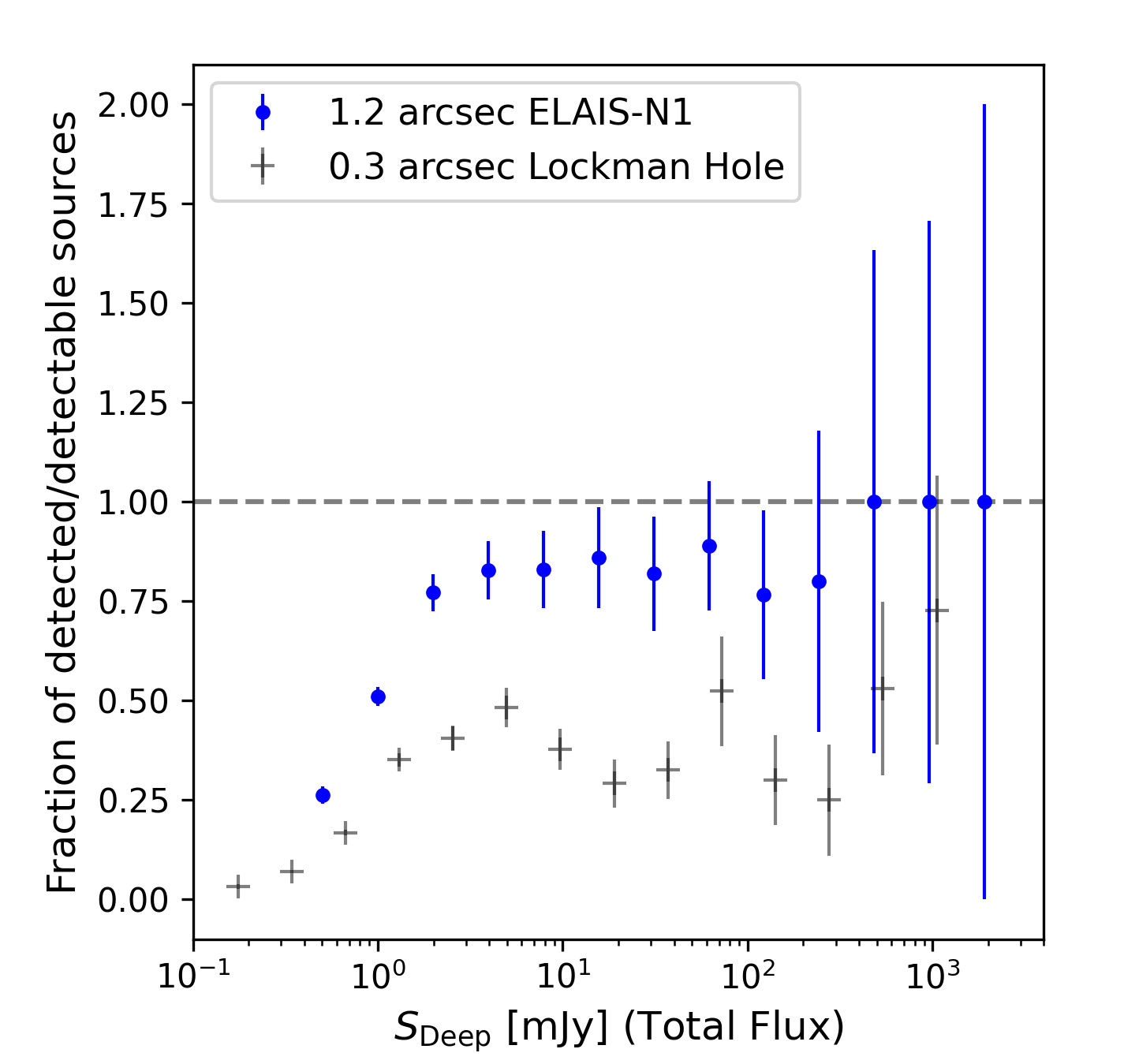
Figure 12: This plot shows the ratio of detected to detectable sources in the 1.2″image, as a function of flux density (from the 6″LoTSS Deep Field catalogue). Sources from the 6″LOFAR deep field ELAIS-N1 catalogue are considered detectable if their peak intensity exceeds 5.5 times the RMS at the same coordinates in our 1.2″ELAIS-N1 image. The blue dots demonstrate this ratio. Uncertainties are estimated using the $\sqrt{N}$ method and propagated accordingly.

We investigated the likelihood that a source in the 6″LOFAR deep field will be detected at higher resolution. This will depend on the amount of flux density which is in compact components and will change as a function of integrated flux density as the population shifts from star-forming galaxies and radio-quiet AGN to radio-loud AGN.

In Figure 12, the blue solid circles depict the ratios of sources detected in the 1.2″image to those that should be detectable based on their peak intensity in the 6″LOFAR deep field ELAIS-N1 radio catalogue. A source is considered detectable if its peak intensity is greater than 5.5 times the RMS at the same coordinates in our 1.2″ELAIS-N1 image. To analyze the results further, sources are separated into different flux bins based on their total flux density. For each bin, the percentage of detected sources is then calculated. The uncertainties on the plot are estimated using the $\sqrt{N}$ method, which considers the number of sources in each bin, and propagates accordingly. It is expected that bright and compact sources are more easily detectable than dim and extended sources.

In contrast, the black crosses represent the same ratio of detected to detectable sources, but this data corresponds to the 0.3″wide-field image of the Lockman Hole, which can be referred to Fig. 8 of the study by Morabito et al. (2022b). Although these are different fields, we can make a general comparison of detection rates at 0.3″and 1.2″; we note that the fields had the same observational setup and data processing strategy up to the point of imaging.

It is immediately obvious that more sources are detected in the 1.2″image at all total flux densities, by a factor of $\sim$2, except for the very highest flux bin ($\sim$1 Jy). The larger quantities of sources detected in the 1.2″image underscores its significance for population studies. We do not see significant evidence for the dip around 5 mJy as seen from the 0.3″Lockman Hole. This is likely due to the increased sensitivity to low-surface brightness radio emission. For the faint population, the 1.2″image detects more radio emission than the 0.3″image, which is likely due to increased sensitivity to low-surface brightness emission on galactic scales. The 0.3″image is sensitive to more compact emission. For the bright population, the increased sensitivity to low-surface brightness radio emission is likely picking up diffuse emission from low excitation radio galaxies (LERGs), which are the dominant population at intermediate to high flux densities (Best et al. 2023; Morabito et al. 2022b). Together these factors can conspire to erase the dip at 5 mJy as shown in Figure 12 in gray. Future comparison of the 1.2″catalogue with galaxy identifications can help shed light on this.

When considered from the viewpoint of computational cost for the imaging step only, it takes around 6 days to produce a final direction-dependently calibrated 1.2″image from an 8-hour fully-calibrated ILT observation, which can run on a single compute node with a 512 GB RAM and dual 24-core Dual Intel Xeon Gold 5220R with hyper-threading. This is at least one order of magnitude cheaper in terms of core hours compared to making a sub-arcsecond resolution image (Sweijen et al. 2022), and also faster in terms of wall time by a factor of a few. Consequently, even a modestly-sized computing infrastructure could handle large-scale imaging at a manageable cost and within a reasonable time frame. If we include all the calibration steps, it took approximately 52,000 core hours to produce this $1.2\arcsec\times 2\arcsec$ image, which is nearly five times faster than sub-arcsecond imaging which would require $\sim$250,000 core hours.

However, there are three more factors to consider when estimating the total computational cost of a 1.2 arcsecond LoTSS-like survey. First, each pointing in the LoTSS survey is separated by $2.6\times 2.6$ $\mathrm{deg}^{2}$, while our current image size is $2.5\times 2.5$ $\mathrm{deg}^{2}$. This means that the computational cost for each pointing would be slightly higher than our current estimates. Second, the smearing effect could be larger unless we reduce the amount of time and frequency averaging, which would further increase the computational cost. Additionally, we may need to use more pointings to achieve a uniform noise level and seamless imaging, as the small field of view of the international stations would result in a non-uniform noise level across each pointing area. Therefore, additional research is in progress to validate the computational feasibility of making a 1.2″survey using LOFAR.

6 Summary and Conclusions

In this paper, we introduced the first wide ($6.45$ $\mathrm{deg}^{2}$) and deep (median noise of $\sim 80\mu\mathrm{Jy}$ ${\mathrm{beam}}^{--1}$) image at a resolution of $1.2\arcsec\times 2\arcsec$ using the International LOFAR High Band Antennas. This image was produced based on an 8-hour observation at frequencies ranging from 120-168 MHz. We outlined our data reduction process, highlighting the most up-to-date ILT imaging strategy used to produce the direction-dependent calibrated image. This results in the production of a radio source catalogue containing 2 263 sources detected over the ELAIS-N1 field, using a peak intensity threshold of $5.5\sigma$. We have performed a cross-matching of our radio source catalogue with the LoTSS deep ELAIS-N1 field radio catalogue, resulting in the correction of flux density and positional inaccuracies.

A comparison of the detected to detectable sources shows that $\sim$80% of the sources in the ELAIS-N1 Deep Fields catalogue are detected at 1.2″above $\sim$2 mJy, which is a factor of 2 larger than the number of sources detected at 0.3″in the Lockman Hole. This implies there is a wealth of information on 1.2″angular scales, and this catalogue represents a valuable resource for future studies of the ELAIS-N1 field.

From a computational perspective, the production of one $\sim$1″resolution image from an 8-hour ILT observation takes approximately 52,000 core hours, including multiple calibration and imaging steps. Notably, this represents only a fraction of the core hours required for sub-arcsecond imaging. This study thus illustrates the promise of conducting a 1″survey using LOFAR HBA. However, further studies are in progress to validate the computational feasibility of making a 1.2″survey using LOFAR.

Appendix A Images of selected extended sources

Figure 13: Selected extended sources from the 1.2″radio catalogue.

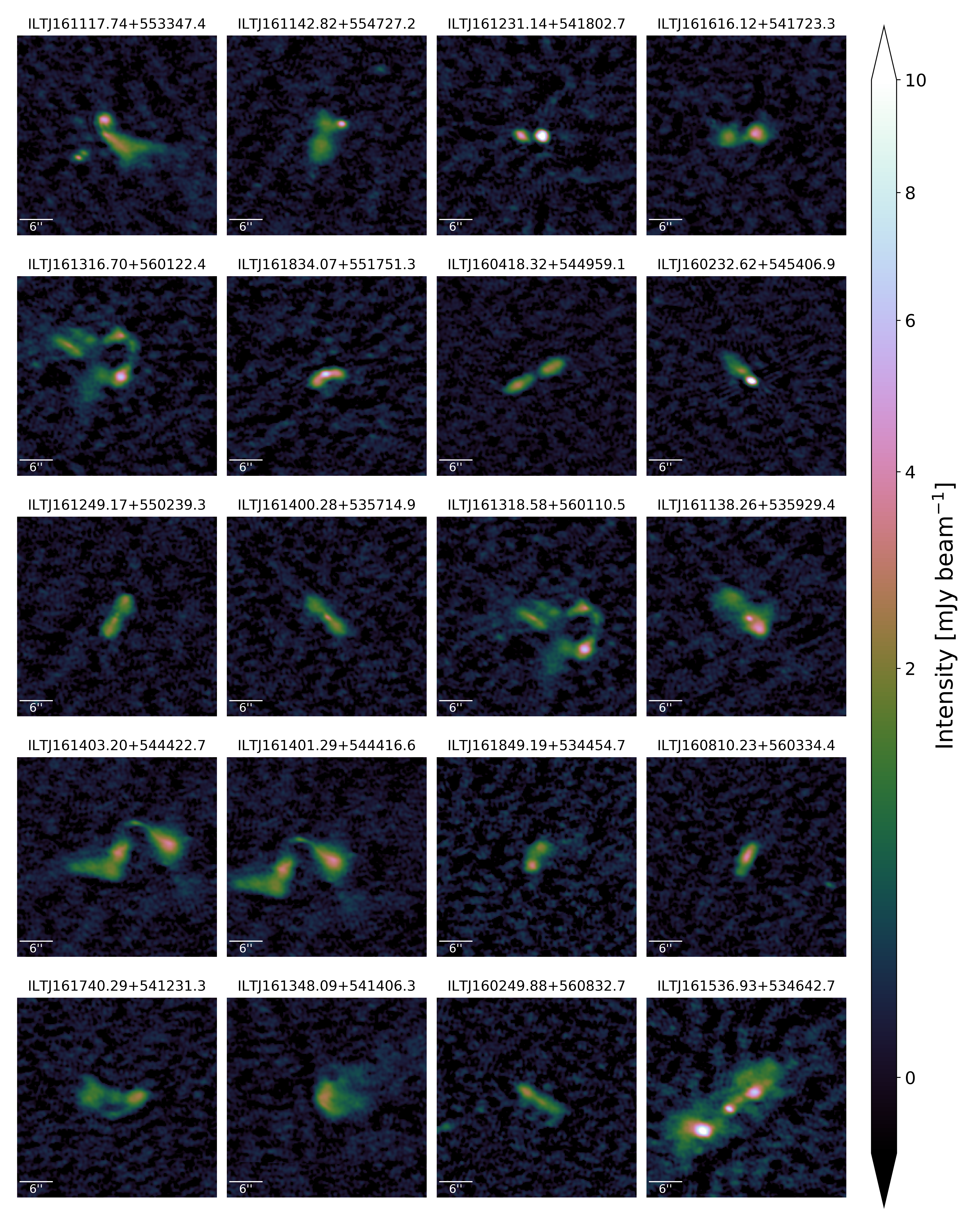
Figure 14: figure

Selected extended sources from the 1.2″radio catalogue.