1 Introduction and main result

Approximation with regular objects is a fundamental tool in many problems in functional analysis and in the Calculus of Variations. For instance, De Giorgi’s theory of sets of finite perimeter depends crucially on the approximability with piecewise smooth sets, a key step in the theory of Sobolev spaces is approximation by smooth functions (for example, the proof of the chain rule depends on it), and similarly for functions of Bounded Variation. Indeed, in these cases a possible definition of the relevant function space is via relaxation of a functional defined on smooth maps, and the difficult part is proving that this is equivalent to the intrinsic definition on measurable sets or functions.

More specifically, approximation and density play an important role in relaxation, $\Gamma$-convergence, integral representation, semicontinuity and many other aspects of the Calculus of Variations in which the topology of the function space is complemented by a variational functional to be minimized. In these applications it is important to approximate in the relevant topology and in energy. In this respect, the literature contains many approximation results for free discontinuity problems, mainly focused on either linear growth or discontinuity sets with finite measure, as appropriate for example for models of concentration of plastic slip or for the Griffith model of brittle fracture. Our main aim here is approximation in energy without the assumption that the jump set has finite measure. One natural application of our result is the study of superlinear models of cohesive fracture.

The functional framework to settle this kind of problems is provided by (a suitable subspace of) the space of Special functions of Bounded Variation, introduced by De Giorgi and Ambrosio in [DGA88] to model a large class of problems which are described by a volume energy and a surface energy (e.g., mixtures of liquids, liquid crystals, image segmentation, fracture mechanics, …). Indeed, $SBV(\mathbb{R}^{n};\mathbb{R}^{m})$ is the set of functions $u\in BV(\mathbb{R}^{n};\mathbb{R}^{m})$ whose distributional derivative has no Cantor part:

$$Du=\nabla u\mathcal{L}^{n}+[u]\otimes\nu_{u}\mathcal{H}^{n-1}\mathop{\hbox{\vrule height=7.0pt,width=0.5pt,depth=0.0pt\vrule height=0.5pt,width=6.0pt,depth=0.0pt}}\nolimits J_{u},$$

where $\nabla u$ is the approximate gradient and $J_{u},\nu_{u},[u]=u^{+}-u^{-}$ are respectively the jump set, its normal, and the amplitude of the jump, see [AFP00] for the definitions.

In these problems, the general form of the energy is

$$F[u,A]:=\int_{A}\Psi(x,\nabla u)dx+\int_{J_{u}\cap A}g(x,u^{+},u^{-},{\nu_{u}})d\mathcal{H}^{n-1},$$ (1.1)

for $A\subset\mathbb{R}^{n}$ open and bounded, $\Psi$ and $g$ satisfying suitable growth and regularity properties, $u\in SBV(A;\mathbb{R}^{m})$. If one is interested in the (possibly constrained) global minimization of $F$, lower semicontinuity and coercivity are further required in order to apply the direct method of the Calculus of Variations and to establish the existence of a solution.

For many applications it is of crucial importance to be able to approximate $u\in SBV(A;\mathbb{R}^{m})$ in $L^{1}(A;\mathbb{R}^{m})$ and in the sense of the energy by a sequence $u_{j}$ of more regular functions (for example piecewise regular), i.e., in a way that $F[u_{j},A]\to F[u,A]$ as $j\to\infty$. This was the aim of several works appeared in the recent years. Braides and Chiadò-Piat in [BCP96, Sect. 5] focus on functions $u\in SBV^{p}\subset SBV$, $p>1$, i.e. such that $\nabla u\in L^{p}$ and $\mathcal{H}^{n-1}(J_{u})<\infty$. For functions $u\in SBV^{p}\cap L^{\infty}$ they provide an approximation $u_{j}\in SBV^{p}$, regular out of a closed rectifiable set, satisfying

$$u_{j}\to u\text{ {strongly} in }BV,\quad\nabla u_{j}\to\nabla u\text{ in }L^{p},\quad\mathcal{H}^{n-1}(J_{u_{j}}\triangle J_{u})\to 0.$$ (1.2)

Cortesani in [Cor97] and Cortesani and Toader in [CT99], on the positive side, improve this result, by constructing for $u\in SBV^{p}{\cap L^{\infty}}$, $p>1$, a sequence $u_{j}$ whose jump set is in addition piecewise regular, and precisely polyhedral. Moreover they get

$$\nabla u_{j}\to\nabla u\text{ in }L^{p},$$

$$\displaystyle\limsup_{j\to\infty}\int_{J_{u_{j}}\cap{\overline{A}}}g(x,u^{+}_{j},u^{-}_{j},\nu_{u_{j}})d\mathcal{H}^{n-1}\leq\int_{J_{u}\cap{\overline{A}}}g(x,u^{+},u^{-},\nu_{u})d\mathcal{H}^{n-1},$$

on $A\subset\subset\Omega$. On the negative side, they do not obtain strong convergence in $SBV$.

The strong convergence in $SBV$ holds for the result by De Philippis, Fusco and Pratelli in [DPFP17, Theorem C], in which, for $u\in SBV^{p}$, $p>1$, the authors construct $u_{j}$ regular out of the closure of its jump set, which is actually essentially closed being contained in a compact $C^{1}$ manifold with $C^{1}$ boundary, and differs from it only by an $\mathcal{H}^{n-1}$-negligible set.

The previous four results have been crucial for many applications involving a penalization on the measure of the jump set. The case in which the jump set of $u$ is allowed to have infinite measure is quite different and few approximations are available in the literature. An extension of the result by Cortesani and Toader to $BV$ was obtained in [ADC05] in the setting of $BV$ strict convergence. In [KR16], the approximation of any $BV$ function is obtained in the area-strict sense through countably piecewise affine functions with the same trace as $u$ at the boundary. A different approximation is provided in $SBV$ in [DPFP17, Theorem B]. Precisely, the authors prove that if $u\in SBV$ with $\nabla u\in L^{p}$, $p>1$, then it is possible to construct $u_{j}$ regular out of the closure of its jump set, which is actually essentially closed being (up to $\mathcal{H}^{n-1}$-null sets) a compact $C^{1}$ manifold with $C^{1}$ boundary, and satisfying

$$u_{j}\to u\text{ {strongly} in }BV,\quad\nabla u_{j}\to\nabla u\text{ in }L^{p}\,.$$

In particular, the convergence $\mathcal{H}^{n-1}(J_{u_{j}}\setminus J_{u})\to 0$ is not ensured. Moreover, in case $p=1$, the jump of $u_{j}$ can be additionally taken contained in the intersection of a compact $C^{1}$ manifold with $C^{1}$ boundary and of the jump set of the function to be approximated (see [DPFP17, Theorem A]). Related density results, with different functional settings such as $(G)SBD$ or $BH$, have been obtained in the last years (see for example [Cha04, Iur14, CFI17, Fri18, FS18, CFI19, Cri19, CC19] and [AABU22, ABC23], respectively).

Although all the quoted results are important advances, they are in general not enough for many applications, not providing any information on the convergence of the surface term or of the total energy $F$ in case that the measure of the jump set is not finite. An easy example is that of an energy $F$ where $\Psi=\Psi(\nabla u)$ is superlinear for large gradients and $g=g([u],\nu_{u})$ is superlinear for small amplitudes, the natural domain of finiteness being (a subset of) $SBV$. In this case, the only result available in the literature is [BCG14, Sect. 4], which however applies only to $u\in GSBV$ with $\nabla u=0$ $\mathcal{L}^{n}$-a.e. on $\Omega$. The approximants satisfy $\nabla u_{j}=0$ $\mathcal{L}^{n}$-a.e. on $\Omega$ and have jump sets of finite measure. The convergence is that of $L^{1}$ together with the convergence of the energies.

In this paper, we develop an original multiscale technique to approximate functions $u\in SBV$ with jump set of possibly infinite measure and $\nabla u\in L^{p}$, with $p\geq 1$. We stress that it encompasses at the same time both superlinear, cohesive-type and Griffith, brittle-type surface energies as shown in Section 2.

Theorem 1.1.

Let $\Omega\subseteq\mathbb{R}^{n}$ be an open bounded Lipschitz set, $u\in SBV(\Omega;\mathbb{R}^{m})$ such that $\nabla u\in L^{p}(\Omega;\mathbb{R}^{m\times n})$ for some $p\in[1,\infty)$, and $g_{0}(|[u]|)\in L^{1}(\Omega;\mathcal{H}^{n-1}\mathop{\hbox{\vrule height=7.0pt,width=0.5pt,depth=0.0pt\vrule height=0.5pt,width=6.0pt,depth=0.0pt}}\nolimits J_{u})$, with $g_{0}:[0,\infty)\to[0,\infty)$ continuous, nondecreasing, subadditive, and $g_{0}^{-1}(0)=\{0\}$.

Then there are sequences $u_{j}\in SBV\cap L^{\infty}(\Omega;\mathbb{R}^{m})$ and $\Phi_{j}\in\mathrm{Lip\,}(\mathbb{R}^{n};\mathbb{R}^{n})$ such that

1. for each $j$ there is a locally finite decomposition of $\mathbb{R}^{n}$ in simplexes such that $u_{j}$ is affine in the interior of each of them;

2. $u_{j}\to u$ in $L^{1}(\Omega;\mathbb{R}^{m})$;

3. $\nabla u_{j}\to\nabla u$ in $L^{p}(\Omega;\mathbb{R}^{m\times n})$;

4. $\Phi_{j}$ is bilipschitz, with $\Phi_{j}(x){-x}\to 0$ in $L^{\infty}(\mathbb{R}^{n};\mathbb{R}^{n})$, ${D}\Phi_{j}\to\mathrm{Id}$ in $L^{\infty}(\mathbb{R}^{n};\mathbb{R}^{n\times n})$, and $\Phi_{j}(x)=x$ for $x\in\mathbb{R}^{n}\setminus\Omega$;

5. one can choose the orientation of the normal $\nu_{j}$ to $J_{u_{j}}$ so that

   $$\lim_{j}\int_{J_{u}\cup\Phi_{j}^{-1}(J_{u_{j}})}g_{0}(|[u]-[u_{j}]\circ\Phi_{j}|)\,d\mathcal{H}^{n-1}=0$$ (1.3)

   (with $[u]=0$ outside $J_{u}$, and similarly for $u_{j}$), and

   $$\lim_{j}\int_{J_{u}\cup\Phi_{j}^{-1}(J_{u_{j}})}g_{0}(|[u]|+|[u_{j}]\circ\Phi_{j}|)\bigl{|}\nu_{u}-\nu_{j}\circ\Phi_{j}\bigr{|}\,d\mathcal{H}^{n-1}=0;$$ (1.4)

6. if $\mathcal{H}^{n-1}(J_{u})<\infty$, then also $\mathcal{H}^{n-1}({J_{u}{\triangle}\Phi_{j}^{-1}(J_{u_{j}})})\to 0$;

7. if $\nabla u=0$ $\mathcal{L}^{n}$-almost everywhere on $\Omega$, then $\nabla u_{j}=0$ $\mathcal{L}^{n}$-almost everywhere on $\Omega$ for all $j$. If instead $u\in W^{1,p}(\Omega;\mathbb{R}^{m})$ then $u_{j}\in W^{1,p}(\Omega;\mathbb{R}^{m})$ for all $j$.

Few remarks are in order. First, since $\Phi_{j}(\Omega)=\Omega$, the integrals in (1.3) and (1.4) are over subsets of $\Omega$. Then, thanks to the subadditivity of $g_{0}$ from items (iv) and (v) it follows that

$$\lim_{j}\int_{J_{u_{j}}}g_{0}(|[u_{j}]|)\,d\mathcal{H}^{n-1}=\int_{J_{u}}g_{0}(|[u]|)\,d\mathcal{H}^{n-1}$$

(see the proof of Corollary 2.1 below). Moreover, under suitable assumptions discussed in details in Section 2, we can deduce the convergence of surface energies with density $g:\mathbb{R}^{m}\times S^{n-1}\to[0,\infty)$ depending suitably on the full jump and the normal. Finally, if $\Psi\in C^{0}(\mathbb{R}^{m\times n})$ has $p$-growth (cf. again Section 2) then (iii) implies

$$\lim_{j}\int_{\Omega}\Psi(\nabla u_{j})\,dx=\int_{\Omega}\Psi(\nabla u)\,dx\,.$$

In addition, the sequence $(u_{j})_{j\in\mathbb{N}}$ can be chosen such that the convergence to $u$ is stronger, namely strict in $BV$ and in area, see Corollary 2.3 below.

We stress that energies with bulk density $\Psi$ and surface density $g$ as above are in general not $L^{1}$ or weakly^∗-$BV$ lower semicontinuous. Hence, our approximations can be used to prove relaxation formulas in the spirit of [Amb89, BC94, BBB95]. This will be the object of future work in [CFI23].

The proof of Theorem 1.1 is obtained through an explicit construction in several steps. First, $u$ can be extended to a function defined on a slightly larger set at a small energy cost. This is not achieved by local reflections at the boundary and a partition of unity process as usually done, which would require $u\in L^{p}$. It is rather pursued through a regularization of the normal vector at the boundary and the definition of a bilipschitz map which swaps an inner neighborhood of the boundary with an outer one. Further details can be found in Section 3.1.

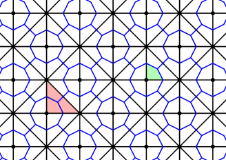
Figure 2: Sketch of the construction for Proposition 4.3. The dots mark the points on which $\Pi_{\varepsilon,\zeta}{f}$ coincides with ${f}$, the black triangles (one of them is colored red) are the elements of $\mathcal{T}_{\varepsilon,\zeta}$, on which Proposition 4.1 is applied. The blue segments are the (eventual) discontinuities introduced by the construction of Proposition 4.1 and delimit the polygons which compose $\mathcal{T}^{*}_{\varepsilon,\zeta}$. The function $\Pi_{\varepsilon,\zeta}u$ is affine on the smaller polyhedra (one of them is colored green).

We employ next a multiscale approach. More precisely, we find a suitable scale $\delta>0$, such that $\nabla u$ is close to a constant and $J_{u}$ is close to a $C^{1}$ manifold in each cube of side $\delta$ of a partition of $\mathbb{R}^{n}$. This is the object of Proposition 3.6. At this point, we introduce a second scale $\varepsilon\ll\delta$. In each cube of side $\delta$ we consider a finer triangulation with simplexes of diameter less than $c\varepsilon$ and volume larger than $c\varepsilon^{n}$. The heart of the paper is Proposition 4.1, which, given the values of $u$ on the vertices of a single simplex, and two vectors for each edge, representing the cumulated jump and the average gradient of $u$ on the edge, provides a piecewise affine interpolation, whose gradient and jump can be estimated respectively only through the given gradient vector or the given jump vector (see Figure 1). Proposition 4.1 is then employed in Proposition 4.3 (see Figure 2) to define a global projection, with good energy estimates, of any $SBV$ function on the space of piecewise affine functions.

The proof of Theorem 1.1 contains a few additional steps, since the direct application of Proposition 4.3 to the given $u$ would provide a piecewise affine approximation with surface energy controlled only up to a multiplicative factor by the surface energy of $u$. To avoid this problem, we first consider the extensions $U^{\pm}$ of $u$ with respect to the $C^{1}$ manifold approximating $J_{u}$ in each cube of side $\delta$. We then apply the previous projection to $U^{\pm}$. We finally introduce a piecewise affine interpolation of the $C^{1}$ manifold and define the approximation of $u$ as the projections of $U^{\pm}$ on the two sides of it. This is performed in the proof of Theorem 1.1 in Section 4.3, see also Figure 3.

The structure of the paper is the following. In Section 2 we provide several consequences of Theorem 1.1, in particular we show that the approximating sequence can be constructed such that it converges also $BV$-strictly, area-strictly and $BV$-strongly after composition with a bilipschitz map. Section 3 addresses two key technical issues: the extension tool in Section 3.1 and the regularization at scale $\delta$ in Section 3.2. Section 4 is devoted to the proof of Theorem 1.1. Precisely, Section 4.1 contains the construction of a relevant piecewise affine interpolation on a single simplex. Section 4.2 applies such construction to produce a piecewise affine approximation of a given $SBV$ function. Finally, Section 4.3 provides the full proof of Theorem 1.1 by applying the projection of Section 4.2 to the extensions of $u$ on the two sides of the regularized jump set and by defining the approximation of $u$ as such projections on the two sides of a suitable perturbation of a piecewise interpolation of the regularized jump set.

2 Consequences of the approximation theorem

We discuss here some consequences of Theorem 1.1. To this aim we fix $p\in[1,\infty)$ and consider $\Psi\in C^{0}(\mathbb{R}^{m\times n})$ obeying for some ${C}>0$,

$${|\Psi(\xi)|\leq{C}(|\xi|^{p}+1).}$$ (2.1)

Throughout the paper $C$ will denote a constant, possibly depending on the dimension (if not otherwise specified) and changing from line to line. Next we select a function $g_{0}:[0,\infty)\to[0,\infty)$ which represents a modulus of continuity of the surface energy $g$ introduced below (see in particular (2.4)) satisfying:

• $g_{0}$ is continuous, nondecreasing, and $g_{0}^{-1}(0)=\{0\}$,

• $g_{0}$ is subadditive, namely for every $(t,t^{\prime})\in[0,\infty)\times[0,\infty)$

  $$g_{0}(t+t^{\prime})\leq g_{0}(t)+g_{0}(t^{\prime})\,.$$

For example either $g_{0}(t)=1\wedge t^{q}$ or $g_{0}(t)=t^{q}$, for $q\in(0,1]$, will do. Note that by subadditivity and continuity of $g_{0}$ in zero, for every $\lambda>0$ there is $C_{\lambda}>0$ such that for all $t\in[0,\infty)$

$$g_{0}(t)\leq\lambda+C_{\lambda}{t}.$$ (2.2)

Then we consider any function $g\in C^{0}(\mathbb{R}^{m}\times S^{n-1};[0,\infty))$, such that

• $g(-s,-\nu)=g(s,\nu)$ for all $(s,\nu)\in\mathbb{R}^{m}\times S^{n-1}$;

• for all $(s,s^{\prime},\nu)\in\mathbb{R}^{m}\times\mathbb{R}^{m}\times S^{n-1}$

  $$g(s+s^{\prime},\nu)\leq g(s,\nu)+{C}\,g_{0}(|s^{\prime}|);$$ (2.3)

and either

• $g(0,\nu)=0$ for all $\nu\in S^{n-1}$

or

• there is $\alpha>0$ such that $g(0,\nu)\geq\alpha$ for all $\nu\in S^{n-1}$.

Thanks to assumption (H${}^{g}_{1}$)​, the surface energy with density $g$ is well defined as it does not depend on the chosen orientation of the normal to the jump set. Assumption (H${}^{g}_{3}$)​ is useful to model cohesive-type energies, such as for example the one of the Barenblatt model. Assumption (H${}^{g}_{3^{\prime}}$)​ is instead useful for surface energies typical of brittle fracture, such as the one of the Griffith model (or, in the scalar case, of the Mumford-Shah model) for which $g$ is constant.

Exchanging the roles of $s$ and $s+s^{\prime}$ in (2.3) yields that

$$|g(s+s^{\prime},\nu)-g(s,\nu)|\leq{C}\,g_{0}(|s^{\prime}|).$$ (2.4)

Moreover, if (H${}^{g}_{3}$)​ holds, the latter estimate with $s^{\prime}=-s$ implies that for all $(s,\nu)\in\mathbb{R}^{m}\times S^{n-1}$

$$g(s,\nu)\leq{C}\,g_{0}(|s|)\,.$$ (2.5)

If instead (H${}^{g}_{3^{\prime}}$)​ holds, then by continuity there is also $\beta>0$ such that $g(0,\nu)\leq\beta$ for all $\nu$, and in particular for all $(s,\nu)\in\mathbb{R}^{m}\times S^{n-1}$

$$g(s,\nu)\leq\beta+{C}\,g_{0}(|s|).$$ (2.6)

For $u\in SBV(\Omega;\mathbb{R}^{m})$ and for a Borel set $A\subseteq\Omega$, we define the energy

$$E_{\Psi,g}[u,A]:=\int_{A}\Psi(\nabla u)dx+\int_{J_{u}\cap A}g([u],{\nu_{u}})d\mathcal{H}^{n-1}\,,$$

where for any $u\in SBV(\Omega;\mathbb{R}^{m})$ we denote by $[u]$ the function which is the usual jump of $u$ on $J_{u}$ and 0 on $\Omega\setminus J_{u}$.

Corollary 2.1.

Under the assumptions of Theorem 1.1, the sequence $(u_{j})_{j\in\mathbb{N}}$ introduced there satisfies

$$\lim_{j}\int_{\Omega}\Psi(\nabla u_{j})dx=\int_{\Omega}\Psi(\nabla u)dx\,,$$ (2.7)

$$\lim_{j}\int_{J_{u_{j}}}g([u_{j}],\nu_{u_{j}})d\mathcal{H}^{n-1}=\int_{J_{u}}g([u],\nu_{u})d\mathcal{H}^{n-1}$$ (2.8)

for all functions $\Psi\in C^{0}(\mathbb{R}^{m\times n})$ satisfying (2.1), and all $g\in C^{0}(\mathbb{R}^{m}\times S^{n-1};[0,\infty))$ satisfying (H${}^{g}_{1}$)​, (H${}^{g}_{2}$)​, and (H${}^{g}_{3}$)​. In particular,

$$\lim_{j}E_{\Psi,g}[u_{j},\Omega]=E_{\Psi,g}[u,\Omega]\,.$$

We stress that the assumptions of Theorem 1.1 include in particular integrability of $g_{0}(|[u]|)$ and ensure via (2.1) and (2.5) that $E_{\Psi,g}[u,\Omega]$ is finite.

Proof.

Standing the $L^{p}$ convergence of $(\nabla u_{j})_{j\in\mathbb{N}}$ to $\nabla u$, we may consider a subsequence, which we do not relabel, such that

$$\limsup_{j}\left|\int_{\Omega}(\Psi(\nabla u_{j})-\Psi(\nabla u))dx\right|$$

is actually a limit, and $(\nabla u_{j})_{j\in\mathbb{N}}$ converges to $\nabla u$ $\mathcal{L}^{n}$-almost everywhere on $\Omega$. Thanks to Egorov’s theorem, for every $\varepsilon>0$ there is $E$ with $|\Omega\setminus E|\leq\varepsilon$ such that $\nabla u\in L^{\infty}(E;\mathbb{R}^{m\times n})$ and $(\nabla u_{j})_{j\in\mathbb{N}}$ converges to $\nabla u$ uniformly on $E$. Therefore, we may use (2.1) and item (iii) in Theorem 1.1 to get

$$\limsup_{j} \left|\int_{\Omega}(\Psi(\nabla u_{j})-\Psi(\nabla u))dx\right|=\limsup_{j}\left|\int_{\Omega\setminus E}(\Psi(\nabla u_{j})-\Psi(\nabla u))dx\right|$$

$$\leq C\Big{(}\int_{\Omega\setminus E}|\nabla u|^{p}dx+|\Omega\setminus E|\Big{)}\,.$$

The conclusion then follows as $\varepsilon\downarrow 0$ by absolute continuity. As the limit is unique, convergence holds for the entire sequence.

We next deal with (2.8). To this aim we first use the Area formula (cf. [AFP00, Theorem 2.91], with $f=\Phi_{j}$ and $E=\Phi_{j}^{-1}(J_{u_{j}})$) which reads

$$\int_{J_{u_{j}}}g([u_{j}],\nu_{u_{j}})d\mathcal{H}^{n-1}=\int_{\Phi_{j}^{-1}(J_{u_{j}})}g([u_{j}]\circ\Phi_{j},\nu_{u_{j}}\circ\Phi_{j}){{\bf J}_{n-1}d^{\Phi_{j}^{-1}(J_{u_{j}})}\Phi_{j}}d\mathcal{H}^{n-1}.$$ (2.9)

We write ${{\bf J}_{n-1}d^{\Phi_{j}^{-1}(J_{u_{j}})}\Phi_{j}}$ for the tangential Jacobian and remark that if $\Phi_{j}$ is differentiable then ${\bf J}_{n-1}d^{\Phi_{j}^{-1}(J_{u_{j}})}\Phi_{j}=|\mathrm{cof}({D}\Phi_{j})(\nu_{u_{j}}\circ\Phi_{j})|$. For $\mathcal{H}^{n-1}$-almost every $x\in\Phi_{j}^{-1}(J_{u_{j}})$, the map $\Phi_{j}$ is differentiable in $x$ in the directions of the tangent space. The same holds for $y\mapsto\Phi_{j}(y)-y$, which is Lipschitz with Lipschitz constant bounded by $\|{D}\Phi_{j}-\mathrm{Id}\|_{L^{\infty}(\mathbb{R}^{n})}$. Therefore for $\mathcal{H}^{n-1}$-almost every $x\in\Phi_{j}^{-1}(J_{u_{j}})$ we have $|{\bf J}_{n-1}d^{\Phi_{j}^{-1}(J_{u_{j}})}\Phi_{j}-1|(x)\leq C\|{D}\Phi_{j}-\mathrm{Id}\|_{L^{\infty}(\mathbb{R}^{n})}$. By (iv), the last expression converges to 0.

We observe that by subadditivity of $g_{0}$

$$\begin{split}&\int_{\Phi_{j}^{-1}(J_{u_{j}})}g_{0}(|[u_{j}]\circ\Phi_{j}|)d\mathcal{H}^{n-1}\\ &\leq\int_{J_{u}\cup\Phi_{j}^{-1}(J_{u_{j}})}g_{0}(|[u]-[u_{j}]\circ\Phi_{j}|)\,d\mathcal{H}^{n-1}+\int_{J_{u}}g_{0}(|[u]|)\,d\mathcal{H}^{n-1}.\end{split}$$

Using (1.3) and the assumption that $g_{0}(|[u]|)\in L^{1}(\Omega,\mathcal{H}^{n-1}\mathop{\hbox{\vrule height=7.0pt,width=0.5pt,depth=0.0pt\vrule height=0.5pt,width=6.0pt,depth=0.0pt}}\nolimits J_{u})$ we obtain that

$$\int_{\Phi_{j}^{-1}(J_{u_{j}})}g_{0}(|[u_{j}]\circ\Phi_{j}|)d\mathcal{H}^{n-1}\leq C<\infty$$ (2.10)

for all $j$. By (2.9), the growth condition in (2.5), and the last step (2.10), we obtain

$$\left|\int_{J_{u_{j}}}g([u_{j}],\nu_{u_{j}})d\mathcal{H}^{n-1}-\int_{\Phi_{j}^{-1}(J_{u_{j}})}g([u_{j}]\circ\Phi_{j},\nu_{u_{j}}\circ\Phi_{j})d\mathcal{H}^{n-1}\right|$$

$$\leq{\|1-{{\bf J}_{n-1}d^{\Phi_{j}^{-1}(J_{u_{j}})}\Phi_{j}}\|_{L^{\infty}(\Phi_{j}^{-1}(J_{u_{j}});\mathcal{H}^{n-1})}}\int_{\Phi_{j}^{-1}(J_{u_{j}})}g([u_{j}]\circ\Phi_{j},\nu_{u_{j}}\circ\Phi_{j})d\mathcal{H}^{n-1}$$

$$\leq o(1)\int_{\Phi_{j}^{-1}(J_{u_{j}})}g_{0}(|[u_{j}]\circ\Phi_{j}|)d\mathcal{H}^{n-1}=o(1)\,.$$ (2.11)

Using (1.3) and (1.4) in Theorem 1.1 and the fact that $g_{0}$ is nondecreasing with $g_{0}^{-1}(0)=\{0\}$ we deduce $\chi_{\Phi_{j}^{-1}(J_{u_{j}})}\to 1$ and $\nu_{u_{j}}\circ\Phi_{j}\to\nu_{u}$, $\mathcal{H}^{n-1}$-almost everywhere on $J_{u}$. Thus, $\chi_{\Phi_{j}^{-1}(J_{u_{j}})}\nu_{u_{j}}\circ\Phi_{j}\to\nu_{u}$, $\mathcal{H}^{n-1}$-almost everywhere on $J_{u}$. Dominated convergence, which we can use by (2.5) and integrability of $g_{0}(|[u]|)$, then yields

$$\limsup_{j}\int_{J_{u}{\cap\Phi_{j}^{-1}(J_{u_{j}})}}\left|g([u],\nu_{u_{j}}\circ\Phi_{j})-g([u],\nu_{u})\right|d\mathcal{H}^{n-1}=0.$$ (2.12)

Moreover, (1.3) in Theorem 1.1(v) yields (with (2.5)) that

$$\limsup_{j}\left(\int_{J_{u}\setminus\Phi_{j}^{-1}(J_{u_{j}})}g([u],\nu_{u})d\mathcal{H}^{n-1}+\int_{\Phi_{j}^{-1}(J_{u_{j}})\setminus J_{u}}g([u_{j}]\circ\Phi_{j},\nu_{u_{j}}\circ\Phi_{j})d\mathcal{H}^{n-1}\right)=0.$$ (2.13)

Therefore, we conclude that

$$\limsup_{j}\left|\int_{J_{u_{j}}}g([u_{j}],\nu_{u_{j}})d\mathcal{H}^{n-1}-\int_{J_{u}}g([u],\nu_{u})d\mathcal{H}^{n-1}\right|$$

$$\leq\limsup_{j}\left|\int_{\Phi_{j}^{-1}(J_{u_{j}})}g([u_{j}]\circ\Phi_{j},\nu_{u_{j}}\circ\Phi_{j})d\mathcal{H}^{n-1}-\int_{J_{u}}g([u],\nu_{u})d\mathcal{H}^{n-1}\right|$$

$$\leq\limsup_{j}\int_{\Phi_{j}^{-1}(J_{u_{j}})\cap J_{u}}\big{|}g([u_{j}]\circ\Phi_{j},{\nu_{u_{j}}\circ\Phi_{j}})-g([u],\nu_{u})\big{|}d\mathcal{H}^{n-1}$$

$${\leq\limsup_{j}\int_{\Phi_{j}^{-1}(J_{u_{j}})\cap J_{u}}\big{|}g([u_{j}]\circ\Phi_{j},{\nu_{u_{j}}\circ\Phi_{j}})-g([u],{\nu_{u_{j}}\circ\Phi_{j}})\big{|}d\mathcal{H}^{n-1}}$$

$$\leq{C}\limsup_{j}\int_{\Phi_{j}^{-1}(J_{u_{j}})\cap J_{u}}\,g_{0}(|[u]-[u_{j}]\circ\Phi_{j}|)\,d\mathcal{H}^{n-1}=0\,,$$

where we have used (2) in the first inequality, (2.13) in the second one, (2.12) in the third one, (2.4) in the fourth one, and (1.3) in Theorem 1.1(v) in the last equality. ∎

We next show how to treat the case that $g$ is bounded from below, in which (H${}^{g}_{3^{\prime}}$)​ holds. We stress that the case of the Mumford-Shah energy functional corresponds to the choices $\Psi=|\cdot|^{2}$ and $g\equiv 1$ as ${|[u]|}>0$ on $J_{u}$ for $u\in SBV$.

Corollary 2.2.

Under the assumptions of Theorem 1.1, if $\mathcal{H}^{n-1}(J_{u})<\infty$ the sequence $(u_{j})_{j\in\mathbb{N}}$ introduced there satisfies

$$\lim_{j}\int_{\Omega}\Psi(\nabla u_{j})dx=\int_{\Omega}\Psi(\nabla u)dx\,,$$ (2.14)

$$\lim_{j}\int_{J_{u_{j}}}g([u_{j}],\nu_{u_{j}})d\mathcal{H}^{n-1}=\int_{J_{u}}g([u],\nu_{u})d\mathcal{H}^{n-1}$$ (2.15)

for all functions $\Psi\in C^{0}(\mathbb{R}^{m\times n})$ satisfying (2.1), and $g\in C^{0}(\mathbb{R}^{m}\times S^{n-1};[0,\infty))$ satisfying (H${}^{g}_{1}$)​, (H${}^{g}_{2}$)​, and (H${}^{g}_{3^{\prime}}$)​. In particular,

$$\lim_{j}E_{\Psi,g}[u_{j},\Omega]=E_{\Psi,g}[u,\Omega]\,.$$

Proof.

The proof is very similar to the one of Corollary 2.1. The first part, until (2.10), is identical. Using (2.6), $\mathcal{H}^{n-1}(J_{u})<\infty$, (vi) in Theorem 1.1, and (2.10) we have

$$\begin{split}&\int_{\Phi_{j}^{-1}(J_{u_{j}})}g([u_{j}]\circ\Phi_{j},\nu_{u_{j}}\circ\Phi_{j})d\mathcal{H}^{n-1}\\ &\leq\beta(\mathcal{H}^{n-1}(J_{u})+\mathcal{H}^{n-1}(\Phi_{j}^{-1}(J_{u_{j}})\setminus J_{u}))+{C}\int_{\Phi_{j}^{-1}(J_{u_{j}})}g_{0}(|[u_{j}]\circ\Phi_{j}|)d\mathcal{H}^{n-1}\\ &\leq C<\infty\end{split}$$ (2.16)

for all $j$. We use the latter and (2.9) to conclude that

$$\left|\int_{J_{u_{j}}}g([u_{j}],\nu_{u_{j}})d\mathcal{H}^{n-1}-\int_{\Phi_{j}^{-1}(J_{u_{j}})}g([u_{j}]\circ\Phi_{j},\nu_{u_{j}}\circ\Phi_{j})d\mathcal{H}^{n-1}\right|$$

$$\leq{\|1-{{\bf J}_{n-1}d^{\Phi_{j}^{-1}(J_{u_{j}})}\Phi_{j}}\|_{L^{\infty}(\Phi_{j}^{-1}(J_{u_{j}});\mathcal{H}^{n-1})}}\int_{\Phi_{j}^{-1}(J_{u_{j}})}g([u_{j}]\circ\Phi_{j},\nu_{u_{j}}\circ\Phi_{j})d\mathcal{H}^{n-1}$$

$$=o(1)$$ (2.17)

which replaces (2). Using (vi) in Theorem 1.1, $\chi_{\Phi_{j}^{-1}(J_{u_{j}})}\to 1$ pointwise $\mathcal{H}^{n-1}$-almost everywhere on $J_{u}$. As above, $\chi_{\Phi_{j}^{-1}(J_{u_{j}})}\nu_{u_{j}}\circ\Phi_{j}\to\nu_{u}$ $\mathcal{H}^{n-1}$-almost everywhere on $J_{u}$. From $\mathcal{H}^{n-1}(J_{u})<\infty$ and integrability of $g_{0}(|[u]|)$ we obtain that $\beta+g_{0}(|[u]|)\in L^{1}(\Omega;\mathcal{H}^{n-1}\mathop{\hbox{\vrule height=7.0pt,width=0.5pt,depth=0.0pt\vrule height=0.5pt,width=6.0pt,depth=0.0pt}}\nolimits J_{u})$. Dominated convergence, which we can use by (2.6), then yields

$$\limsup_{j}\int_{J_{u}{\cap\Phi_{j}^{-1}(J_{u_{j}})}}\left|g([u],\nu_{u_{j}}\circ\Phi_{j})-g([u],\nu_{u})\right|d\mathcal{H}^{n-1}=0.$$ (2.18)

Moreover, items (v) and (vi) in Theorem 1.1 and (2.6), yield that

$$\limsup_{j}\left(\int_{J_{u}\setminus\Phi_{j}^{-1}(J_{u_{j}})}g([u],\nu_{u})d\mathcal{H}^{n-1}+\int_{\Phi_{j}^{-1}(J_{u_{j}})\setminus J_{u}}g([u_{j}]\circ\Phi_{j},\nu_{u_{j}}\circ\Phi_{j})d\mathcal{H}^{n-1}\right)=0.$$ (2.19)

The rest of the proof is unchanged. ∎

We can actually strengthen the conclusions of Corollary 2.1 and Corollary 2.2 by constructing an approximating sequence converging in a stronger sense.

Corollary 2.3.

In Corollary 2.1 and Corollary 2.2 the sequence $(u_{j})_{j\in\mathbb{N}}$ can be chosen to additionally satisfy

$${\lim_{j}|(\Phi_{j})_{\#}Du_{j}-Du|(\Omega)=0}$$ (2.20)

and

$$\lim_{j}\|u_{j}\circ\Phi_{j}-u\|_{BV(\Omega)}=0\,.$$ (2.21)

In particular,

$$\lim_{j}\int_{\Omega}|\nabla u_{j}|dx=\int_{\Omega}|\nabla u|dx\,,$$ (2.22)

$$\lim_{j}\int_{\Omega}\sqrt{1+|\nabla u_{j}|^{2}}dx=\int_{\Omega}\sqrt{1+|\nabla u|^{2}}dx\,,$$ (2.23)

$$\lim_{j}\int_{J_{u_{j}}}|[u_{j}]|d\mathcal{H}^{n-1}=\int_{J_{u}}|[u]|d\mathcal{H}^{n-1}\,,$$ (2.24)

so that $(u_{j})_{j\in\mathbb{N}}$ converges to $u$ strictly in $BV(\Omega;\mathbb{R}^{m})$ and in area.

Proof.

The proof is based on the fact that the construction of the sequence in Theorem 1.1 does not depend on the details of the energy considered. We define the auxiliary functions $\widetilde{g}_{0}:{[0,\infty)}\to[0,\infty)$, $\widetilde{g}:\mathbb{R}^{m}\to[0,\infty)$, by

$$\widetilde{g}_{0}(t):=g_{0}(t)+t\,,\hskip 14.22636pt{t\in[0,\infty)\,,}$$

and

$$\widetilde{g}(s):=|s|\,,\hskip 14.22636pt{s\in\mathbb{R}^{m}\,.}$$

It is easy to check that $\widetilde{g}_{0}$ satisfies (H${}^{g_{0}}_{1}$​)-(H${}^{g_{0}}_{2}$​), and moreover that both $g$ and $\widetilde{g}$ satisfy (H${}^{g}_{1}$)​-(H${}^{g}_{2}$)​ with respect to $\widetilde{g}_{0}$. Further, $\widetilde{g}$ satisfies (H${}^{g}_{3}$)​. In addition, if $u\in SBV(\Omega;\mathbb{R}^{m})$, having assumed that $g_{0}(|[u]|)\in L^{1}(\Omega;\mathcal{H}^{n-1}\mathop{\hbox{\vrule height=7.0pt,width=0.5pt,depth=0.0pt\vrule height=0.5pt,width=6.0pt,depth=0.0pt}}\nolimits J_{u})$, we infer that $\widetilde{g}_{0}(|[u]|)\in L^{1}(\Omega;\mathcal{H}^{n-1}\mathop{\hbox{\vrule height=7.0pt,width=0.5pt,depth=0.0pt\vrule height=0.5pt,width=6.0pt,depth=0.0pt}}\nolimits J_{u})$. Therefore, we may consider the sequence $(u_{j})_{j\in\mathbb{N}}$ provided by Theorem 1.1 with surface density $\widetilde{g}_{0}$. Thus, to get (2.22)–(2.24) it is sufficient to apply Corollary 2.1 with $\Psi_{1}(\xi):=|\xi|$ and $\widetilde{g}$, and then $\Psi_{2}(\xi):=\sqrt{1+|\xi|^{2}}$ and $\widetilde{g}$. One applies either Corollary 2.1 or Corollary 2.2 with densities $\Psi$ and $g$ to obtain convergence of the energy. From Theorem 1.1(v) for $\tilde{g}_{0}$ we obtain

$${\lim_{j}\int_{J_{u}\cup\Phi_{j}^{-1}(J_{u_{j}})}|[u_{j}]\circ\Phi_{j}-[u]|d\mathcal{H}^{n-1}=0\,,}$$

and with (iii) and (iv) we conclude $|(\Phi_{j})_{\#}Du_{j}-Du|(\Omega)\to 0$. It remains to prove (2.21). Recalling Theorem 1.1 (ii) and (iv) and (2.20), it is enough to check that

$$\lim_{j}\int_{\Omega}|\nabla(u_{j}\circ\Phi_{j})-\nabla u|dx=0.$$

Let ${\mathcal{S}_{j}}$ be the decomposition of Theorem 1.1 (i), then $u_{j}$ is affine in $T$, for all $T\in{\mathcal{S}_{j}}$, and the chain rule gives

$$\displaystyle\int_{\Omega}|\nabla(u_{j}\circ\Phi_{j})-\nabla u|dx=\sum_{T\in{\mathcal{S}_{j}}}\int_{\Omega\cap\Phi_{j}^{-1}(T)}|\nabla(u_{j}\circ\Phi_{j})-\nabla u|dx$$

$$=\displaystyle\sum_{T\in{\mathcal{S}_{j}}}\int_{\Omega\cap\Phi_{j}^{-1}(T)}|(\nabla u_{j}\circ\Phi_{j}){D}\Phi_{j}-\nabla u|dx.$$

The triangular inequality yields

$$\int_{\Omega\cap\Phi_{j}^{-1}(T)}|(\nabla u_{j}\circ\Phi_{j}){D}\Phi_{j}-\nabla u|dx\leq\int_{\Omega\cap\Phi_{j}^{-1}(T)}|\nabla u_{j}\circ\Phi_{j}||{D}\Phi_{j}-\mathrm{Id}|dx\\ +\int_{\Omega\cap\Phi_{j}^{-1}(T)}|(\nabla u_{j}-\nabla u)\circ\Phi_{j}|dx+\int_{\Omega\cap\Phi_{j}^{-1}(T)}|\nabla u\circ\Phi_{j}-\nabla u|dx$$

and all terms tend to zero by Theorem 1.1 (iv) and (2.20). This gives the conclusion. ∎

Finally, we extend the above approximation results to functions belonging to $(GSBV(\Omega))^{m}$ with energy $E_{|\cdot|^{p},g_{0}}$ finite (we refer to [AFP00, Section 4.5] for the basic notation and theory).

Corollary 2.4.

Let $\Omega\subseteq\mathbb{R}^{n}$ be an open bounded Lipschitz set, $u\in L^{1}(\Omega;\mathbb{R}^{m})\cap(GSBV(\Omega))^{m}$ be such that $\nabla u\in L^{p}(\Omega;\mathbb{R}^{m\times n})$ for some $p\in[1,\infty)$, and $g_{0}(|[u]|)\in L^{1}(\Omega;\mathcal{H}^{n-1}\mathop{\hbox{\vrule height=7.0pt,width=0.5pt,depth=0.0pt\vrule height=0.5pt,width=6.0pt,depth=0.0pt}}\nolimits J_{u})$, with $g_{0}:[0,\infty)\to[0,\infty)$ continuous, nondecreasing, subadditive, and $g_{0}^{-1}(0)=\{0\}$.

Then, there exists a sequence $(u_{j})_{j\in\mathbb{N}}\subseteq SBV\cap L^{\infty}(\Omega;\mathbb{R}^{m})$ such that all the conclusions in Theorem 1.1 hold, and in addition

$$\lim_{j}\int_{\Omega}\Psi(\nabla u_{j})dx=\int_{\Omega}\Psi(\nabla u)dx\,,$$ (2.25)

$$\lim_{j}\int_{J_{u_{j}}}g([u_{j}],\nu_{u_{j}})d\mathcal{H}^{n-1}=\int_{J_{u}}g([u],\nu_{u})d\mathcal{H}^{n-1}$$ (2.26)

for all functions $\Psi\in C^{0}(\mathbb{R}^{m\times n})$ satisfying (2.1), and all $g\in C^{0}(\mathbb{R}^{m}\times S^{n-1};[0,\infty))$ satisfying (H${}^{g}_{1}$)​, (H${}^{g}_{2}$)​, and (H${}^{g}_{3}$)​. In addition, if $\mathcal{H}^{n-1}(J_{u})<\infty$, (2.26) holds for all $g\in C^{0}(\mathbb{R}^{m}\times S^{n-1};[0,\infty))$ satisfying (H${}^{g}_{1}$)​, (H${}^{g}_{2}$)​, and (H${}^{g}_{3^{\prime}}$)​.

Moreover, the sequence $(u_{j})_{j\in\mathbb{N}}$ can be chosen such that (2.22) and (2.23) hold.

Proof.

We argue by density by constructing a sequence $(\tilde{u}_{k})_{k\in\mathbb{N}}\subset SBV\cap L^{\infty}(\Omega;\mathbb{R}^{m})$ converging in $L^{1}(\Omega;\mathbb{R}^{m})$ and in energy to $u$. This is well-known nowadays, in any case for the readers’ convenience we recall the definition. To this aim we fix a sequence $(a_{k})_{k\in\mathbb{N}}\subset(0,\infty)$ such that $a_{k}<a_{k+1}$, $a_{k}\uparrow\infty$, and such that there are functions $\mathcal{T}_{k}\in{C^{1}_{c}}(\mathbb{R}^{n};\mathbb{R}^{m})$ satisfying $\mathcal{T}_{k}(z){=z}$ if $|z|\leq a_{k}$, $\mathcal{T}_{k}(z)=0$ if $|z|\geq a_{k+1}$, and $\|{D}\mathcal{T}_{k}\|_{L^{\infty}(\mathbb{R}^{n};\mathbb{R}^{m})}\leq 1$. Then, the sequence $\tilde{u}_{k}:=\mathcal{T}_{k}(u){\in SBV(\Omega;\mathbb{R}^{m})}$ converges to $u$ in $L^{1}(\Omega;\mathbb{R}^{m})$, $\nabla\tilde{u}_{k}=\nabla u$ $\mathcal{L}^{n}$-almost everywhere on $\Omega_{k}:=\{x\in\Omega:\,|u(x)|\leq a_{k}\}$, $J_{\tilde{u}_{k}}\subseteq J_{u}$, $\nu_{\tilde{u}_{k}}=\nu_{u}$ $\mathcal{H}^{n-1}$-almost everywhere on $J_{\tilde{u}_{k}}$. Moreover, as

$$\mathcal{H}^{n-1}(\{x\in J_{u}:\,|u^{\pm}(x)|=\infty\})=0$$

(see [AF02, Proposition 2.12, Remark 2.13]) we infer that $\chi_{J_{\tilde{u}_{k}}}\to\chi_{J_{u}}$, $\tilde{u}^{\pm}_{k}(x)=u^{\pm}(x)$ $\mathcal{H}^{n-1}$-almost everywhere on $J_{\tilde{u}_{k}}\cap\Omega_{k}$, $|[\tilde{u}_{k}]|\leq|[u]|$ and $\tilde{u}_{k}^{\pm}\to u^{\pm}$ $\mathcal{H}^{n-1}$-almost everywhere on $J_{u}$. Therefore, we get

$$\lim_{k}\int_{\Omega}|\nabla\tilde{u}_{k}|^{p}dx=\int_{\Omega}|\nabla u|^{p}dx\,,$$

and thanks to the subadditivity and monotonicity properties of $g_{0}$ also that

$$\lim_{k}\int_{J_{u}}g_{0}(|[u]-[\tilde{u}_{k}]|)d\mathcal{H}^{n-1}=0$$

(for detailed proofs of similar properties see, for instance, [AF02, Lemma 6.1] and [CFI22, Proposition 4.8]).

Next, for every $k\in\mathbb{N}$ we apply Theorem 1.1 in order to get a sequence $(\tilde{u}_{k,j})_{j\in\mathbb{N}}$ approximating $\tilde{u}_{k}$ and satisfying all the conditions in that statement. Eventually, we conclude thanks to a diagonalization argument in view of the properties of $g_{0}$, $\Psi$ and $g$ and the arguments in Corollaries 2.1 or 2.2, and in Corollary 2.3. ∎

3 Technical results

In this section we collect the key technical tools we use to prove Theorem 1.1. For $SBV$ functions having finite energy according to Theorem 1.1, we establish first an extension result, and then some measure theoretic properties crucial for our constructions.

3.1 Extension

In this section we prove an extension result for $SBV$ functions. A standard local reflection argument would work for $SBV\cap L^{p}$ functions. However, in the present setting it is not clear that having finite energy implies finiteness of the $L^{p}$ norm. In particular, to the aim of applications, both for approximation via $\Gamma$-convergence and for the determination of relaxation of variational integrals, it is not natural to assume additionally $u\in L^{p}$ (see for example the forthcoming paper [CFI23]), therefore we avoid the extra $L^{p}$ integrability condition. To this aim, we introduce a global reflection argument based on a bilipschitz map reflecting a neighborhood of $\partial\Omega$ in $\Omega$, outside of $\Omega$ itself.

The general strategy is standard, but to the best of our knowledge the details are new. For example, a similar result was obtained in [CS11, Th. 3.1] with a more complex construction using the solution of an ODE (see [CS11, Eq. (3.5)] instead of the specific formula (3.21) below for the construction of the reflection.

Theorem 3.1.

Let $\Omega\subseteq\mathbb{R}^{n}$ be a bounded Lipschitz set. Then there are an open set $\omega\subseteq\mathbb{R}^{n}$ with $\partial\Omega\subset\omega$ and a bilipschitz map $\Phi:\omega\to\omega$ such that $\Phi(x)=x$ for $x\in\partial\Omega$ and $\Phi(\omega\cap\Omega)=\omega\setminus\overline{\Omega}$.

We recall that a map $f:E\to f(E)\subseteq\mathbb{R}^{n}$, for $E\subseteq\mathbb{R}^{n}$, is bilipschitz if there is $L>0$ such that

$$\frac{1}{L}|x-y|\leq|f(x)-f(y)|\leq L|x-y|$$ (3.1)

for all $x,y\in E$. This is the same as saying that $f$ is injective, Lipschitz, with a Lipschitz inverse $f^{-1}:f(E)\to E$.

Moreover, a set $\Omega$ is Lipschitz if for every $x\in\partial\Omega$ there are $\varepsilon_{x}>0$, ${G}_{x}\in\mathrm{Lip\,}(\mathbb{R}^{n-1})$ and an isometry $A_{x}:\mathbb{R}^{n}\to\mathbb{R}^{n}$ such that $A_{x}0=x$ and

$$B_{{\varepsilon_{x}}}(x)\cap\Omega=B_{{\varepsilon_{x}}}(x)\cap A_{x}\{(y^{\prime},y_{n})\in\mathbb{R}^{n-1}\times\mathbb{R}:y_{n}<{G}_{x}(y^{\prime})\}.$$ (3.2)

Obviously ${G}_{x}(0)=0$; if $|y^{\prime}|<\varepsilon_{x}/(\mathrm{Lip\,}({G}_{x})+1)$ then ${A_{x}}(y^{\prime},{{G}_{x}}(y^{\prime}))\in B_{\varepsilon_{x}}{(x)}\cap\partial\Omega$. If $\Omega$ is bounded, there are $\varepsilon_{0}$ and $L_{0}$ such that one can choose $\varepsilon_{x}\geq\varepsilon_{0}$ and $\mathrm{Lip\,}({G}_{x})\leq L_{0}$ for all $x\in\partial\Omega$.

We start with defining a smooth vector field playing the role of the normal field to $\partial\Omega$, which under our hypotheses is only a function in $L^{\infty}(\partial\Omega;S^{n-1})$.

Lemma 3.2.

Let $\Omega\subseteq\mathbb{R}^{n}$ be a bounded Lipschitz set. Then there are $\gamma>0$ and a map $\psi\in C^{\infty}_{c}(\mathbb{R}^{n};\mathbb{R}^{n})$ such that $\psi(x)\cdot\nu(x)\geq\gamma$ for $\mathcal{H}^{n-1}$-almost every $x\in\partial\Omega$ and $|\psi|=1$ on $\partial\Omega$.

This is well-known (see, for example, [CM08, Lemma 4.1]), for completeness we include the short proof.

Proof.

The compact set $\partial\Omega$ can be covered by a finite family of balls $B_{i}:=B_{r_{i}}({z_{i}})$, such that in each of the larger balls $B_{i}^{*}:=B_{2r_{i}}({z_{i}})$ (3.2) reads

$$B_{i}^{*}\cap\Omega=B_{i}^{*}\cap{A_{i}}\{(x^{\prime},x_{n}):x_{n}<{G}_{i}(x^{\prime})\}$$ (3.3)

for some ${G}_{i}\in\mathrm{Lip\,}(\mathbb{R}^{n-1})$ and isometry $A_{i}$. If $x^{\prime}$ is such that $y:={A_{i}}(x^{\prime},{G}_{i}(x^{\prime}))\in\partial\Omega\cap B_{i}^{*}$ and ${G}_{i}$ is differentiable at $x^{\prime}$, then the outer normal obeys $\nu(y)=R_{i}(-D{G}_{i}(x^{\prime}),1)/\sqrt{1+|D{G}_{i}|^{2}(x^{\prime})}$, where $R_{i}:={D}A_{i}\in\mathrm{O}(n)$, so that

$$\nu\cdot R_{i}e_{n}\geq\gamma^{*}:=\frac{1}{\sqrt{1+\max_{i}(\mathrm{Lip\,}({G}_{i}))^{2}}}>0$$ (3.4)

$\mathcal{H}^{n-1}$-almost everywhere on $B_{i}^{*}\cap\partial\Omega$. We fix cutoff functions $\theta_{i}\in C^{\infty}_{c}(B^{*}_{i};[0,1])$ with $\theta_{i}=1$ on $B_{i}$, and set $\psi^{*}(x):=\sum_{i}\theta_{i}(x)R_{i}e_{n}$. Then for $\mathcal{H}^{n-1}$-almost every point $x\in\partial\Omega$ we have

$$\psi^{*}(x)\cdot\nu(x)=\sum_{i:x\in B^{*}_{i}}\theta_{i}(x)(R_{i}e_{n})\cdot\nu(x)\geq\sum_{i:x\in B^{*}_{i}}\theta_{i}(x)\gamma^{*}\geq\gamma^{*},$$ (3.5)

since at least one of the $\theta_{i}(x)$ equals 1.

It only remains to normalize. Condition (3.5) implies $|\psi^{*}|\geq\gamma^{*}$ on $\partial\Omega$, and therefore $|\psi^{*}|>\gamma^{*}/2$ in a neighborhood of $\partial\Omega$. We select $\varphi\in C^{\infty}(\mathbb{R}^{n};[0,1])$ such that $\varphi=0$ on $\partial\Omega$, and $\varphi>0$ on the set $|{\psi^{*}}|\leq\gamma^{*}/2$. Then $\psi:=\psi^{*}/\sqrt{|\psi^{*}|^{2}+\varphi}$ has the desired properties with $\gamma:=\gamma^{*}/\max|\psi^{*}|(\partial\Omega)$. ∎

Lemma 3.3.

Let $\Omega\subseteq\mathbb{R}^{n}$ be a bounded Lipschitz set, $\psi$ as in Lemma 3.2. There are $\rho>0$ and $c>0$ such that for any $x,y\in\partial\Omega$ with $|x-y|<\rho$ one has

$$|x-y|\leq c|(\mathrm{Id}-\psi(y)\otimes\psi(y))(x-y)|.$$ (3.6)

Proof.

We can assume $x\neq y$. After a change of coordinates, and choosing $\rho$ sufficiently small, we can assume that $y=0$, and that

$$\partial\Omega\cap B_{(1+L)\rho}(0)=B_{(1+L)\rho}(0)\cap\{(z^{\prime},{G}(z^{\prime})):z^{\prime}\in\mathbb{R}^{n-1}\}$$ (3.7)

for some $L$-Lipschitz function ${G}:\mathbb{R}^{n-1}\to\mathbb{R}$. The values of $\rho$ and $L$ have bounds that depend only on $\Omega$. Let $m:=\psi(0)$, so that $P:=\mathrm{Id}-m\otimes m$ is the projection onto the space orthogonal to $m$. Condition (3.6) then translates into

$$|x|\leq c|Px|$$ (3.8)

for any $x\in\partial\Omega\cap{B_{\rho}(0)}$. As both sides of (3.8) are continuous, it suffices to prove it for $\mathcal{H}^{n-1}$-almost every $x$. By (3.7), we have $x=(x^{\prime},{G}(x^{\prime}))$ for some $x^{\prime}\in\mathbb{R}^{n-1}\setminus\{0\}$. Define $\hat{x}:={(\hat{x}^{\prime},0):=(\frac{x^{\prime}}{|x^{\prime}|},0)}\in S^{n-2}{\times\{0\}}\subset\mathbb{R}^{n-1}{\times\{0\}}$. Let $\Pi:=\mathrm{span}\{\hat{x},e_{n}\}$, we remark that $\hat{x}\cdot e_{n}=0$ and that $x\in\Pi$. Let $m_{\Pi}$ be the orthogonal projection of $m$ on $\Pi$, namely

$$m_{\Pi}:=(\hat{x}\otimes\hat{x}+e_{n}\otimes e_{n})m=(\hat{x}\cdot m)\hat{x}+(e_{n}\cdot m)e_{n}\in\Pi,$$ (3.9)

and $m_{\perp}:=m-m_{\Pi}$, so that $m=m_{\Pi}+m_{\perp}$. Then, as $x\in\Pi$ and $m_{\perp}\in\Pi^{\perp}$ we have

$$|Px|^{2}=|(\mathrm{Id}-(m_{\Pi}+m_{\perp})\otimes(m_{\Pi}+m_{\perp}))x|^{2}=|x-(m_{\Pi}\cdot x)m_{\Pi}|^{2}+|m_{\perp}|^{2}|m_{\Pi}\cdot x|^{2}.$$ (3.10)

We distinguish two cases. If $|m_{\perp}|\geq\frac{1}{2}\gamma$, with $\gamma$ the constant from Lemma 3.2, the first term leads to

$$|Px|\geq|x-(m_{\Pi}\cdot x)m_{\Pi}|\geq|x|-|m_{\Pi}|^{2}|x|=|m_{\perp}|^{2}|x|\geq\frac{\gamma^{2}}{4}|x|$$ (3.11)

which concludes the proof of (3.8) in this case.

Assume now that $|m_{\perp}|\leq\frac{1}{2}\gamma$. For any $z^{\prime}\in\mathbb{R}^{n-1}$ with $|z^{\prime}|<\rho$ we have $z:=(z^{\prime},{G}(z^{\prime}))\in\partial\Omega\cap B_{\rho(1+L)}(0)$, and if ${G}$ is differentiable in $z^{\prime}$ the outer normal is

$$\nu({z})=\frac{1}{\sqrt{1+|D{G}|^{2}(z^{\prime})}}\begin{pmatrix}-D{G}(z^{\prime})\\ 1\end{pmatrix}.$$ (3.12)

Recalling $\psi(z)\cdot\nu(z)\geq\gamma$,

$$\begin{split}m\cdot\nu{(z)}{=\psi(z)\cdot\nu{(z)}+(\psi(0)-\psi(z))\cdot\nu(z)\geq\gamma-\|\psi\|_{C^{1}}\,|z|}\end{split}$$ (3.13)

so that, if $\rho<\gamma/(4\|\psi\|_{C^{1}}(1+L))$, the condition $|m_{\perp}|\leq\frac{1}{2}\gamma$ implies

$$\begin{split}m_{\Pi}\cdot\nu{(z)}=m\cdot\nu{(z)}-m_{\perp}\cdot\nu{(z)}\geq\gamma-{\frac{1}{4}\gamma}-|m_{\perp}|\geq\frac{1}{4}\gamma.\end{split}$$ (3.14)

By (3.12) and (3.9),

$$m_{\Pi}\cdot\nu(z)=\frac{1}{\sqrt{1+|D{G}|^{2}(z^{\prime})}}\left[(e_{n}\cdot m)-(\hat{x}\cdot m){\hat{x}^{\prime}}\cdot D{G}(z^{\prime})\right].$$ (3.15)

With a slight abuse of notation we have used the dot to denote the inner product both in $\mathbb{R}^{n-1}$ and $\mathbb{R}^{n}$.

Let $\zeta(t):=(t{\hat{x}^{\prime}},{G}(t{\hat{x}^{\prime}}))$, for $t\in[0,|x^{\prime}|]$. For $\mathcal{H}^{n-1}$-almost every choice of $x^{\prime}\in B^{\prime}_{\rho}$ we have that for $\mathcal{H}^{1}$-almost every $t$ the function ${G}$ is differentiable in $t\hat{x}^{\prime}$. Clearly $\zeta(0)=0$, $\zeta(|x^{\prime}|)=x$, and $\zeta$ is Lipschitz with

$$D\zeta(t)=\hat{x}+({\hat{x}^{\prime}\cdot}D{G}(t{\hat{x}^{\prime}}))e_{n}.$$ (3.16)

We define

$$m_{\Pi}^{\perp}:=(e_{n}\otimes\hat{x}-\hat{x}\otimes e_{n})m=(\hat{x}\cdot m)e_{n}-(e_{n}\cdot m)\hat{x}\in\Pi\,,$$ (3.17)

and compute

$$\begin{split}m_{\Pi}^{\perp}\cdot x&=\int_{0}^{|x^{\prime}|}m_{\Pi}^{\perp}\cdot{D\zeta}(t)dt=\int_{0}^{|x^{\prime}|}\left[(\hat{x}\cdot m){(\hat{x}^{\prime}\cdot D{G}(t{\hat{x}^{\prime}}))}-(e_{n}\cdot m)\right]dt.\end{split}$$ (3.18)

Using first (3.15) and then (3.14),

$$\begin{split}m_{\Pi}^{\perp}\cdot x&=-\int_{0}^{|x^{\prime}|}m_{\Pi}\cdot\nu(\zeta(t))\sqrt{1+|D{G}|^{2}({t\hat{x}^{\prime}})}dt\leq-|x^{\prime}|\frac{\gamma}{4}.\end{split}$$ (3.19)

With $|m_{\Pi}^{\perp}|{\leq}1$ and $m_{\Pi}^{\perp}\cdot m=0$ (note that $m_{\Pi}^{\perp}\in\Pi$ and $m_{\Pi}^{\perp}\cdot m_{\Pi}=0$) we obtain

$$|Px|\geq{\left|x\cdot\frac{m_{\Pi}^{\perp}}{|m_{\Pi}^{\perp}|}\right|{\geq}|x\cdot m_{\Pi}^{\perp}|}\geq\frac{\gamma}{4}|x^{\prime}|\,.$$ (3.20)

Recalling that $|x|\leq|x^{\prime}|+|{G}(x^{\prime})|\leq(1+L)|x^{\prime}|$, this concludes the proof of (3.8), and therefore of (3.6) (with $c=4(1+L)/\gamma^{2}$). ∎

We are now ready to prove Theorem 3.1. Before starting, we recall that by Brower’s invariance of domain theorem any injective continuous map $f:E\subseteq\mathbb{R}^{n}\to\mathbb{R}^{n}$ is open, in the sense that if $E$ is open then $f(E)$ is open.

Proof of Theorem 3.1..

Step 1. Let $\psi$ be as in Lemma 3.2, $\rho$ as in Lemma 3.3, and define $f:\partial\Omega\times\mathbb{R}\to\mathbb{R}^{n}$ by

$$f(x,t):=x+t\psi(x).$$ (3.21)

We claim that there are $\varepsilon>0$ and $C>0$, depending only on $\Omega$, such that for all $x,y\in\partial\Omega$, all $t,s\in(-\varepsilon,\varepsilon)$,

$$|x-y|+|t-s|\leq C|f(x,t)-f(y,s)|.$$ (3.22)

In order to prove (3.22) we write

$$f(x,t)-f(y,s)=x-y+t\psi(x)-s\psi(y).$$ (3.23)

We shall choose $\varepsilon\leq\rho$. If $|x-y|\leq\rho$ we can use Lemma 3.3. Let $P_{y}$ be the projection onto $\psi(y)^{\perp}$. Then

$$P_{y}(f(x,t)-f(y,s))=P_{y}(x-y)+tP_{y}(\psi(x)-\psi(y)).$$ (3.24)

For the second term we use $|\psi(x)-\psi(y)|\leq\|\psi\|_{C^{1}}|x-y|$. For the first term, we use (3.6). We then obtain

$$|f(x,t)-f(y,s)| \geq|P_{y}(x-y)|-|t|\,|\psi(x)-\psi(y)|$$

$$\geq\frac{1}{c}|x-y|-\varepsilon\|\psi\|_{C^{1}}|x-y|\geq\frac{1}{2c}|x-y|$$ (3.25)

provided that $\varepsilon\leq 1/(2c\|\psi\|_{C^{1}})$. To estimate $t-s$ we write (3.23) as

$$f(x,t)-f(y,s)=(t-s)\psi(x)+x-y+s(\psi(x)-\psi(y))$$ (3.26)

so that

$$|t-s|\leq|f(x,t)-f(y,s)|+|x-y|+|s|\,\|\psi\|_{C^{1}}\,|x-y|$$ (3.27)

which, recalling that $|s|\|\psi\|_{C^{1}}\leq 1/(2c)$, together with (3.1) concludes the proof of (3.22) in this case.

Assume now that $|x-y|>\rho$, still with $|t|,|s|<\varepsilon$. Then (3.23) gives

$$|f(x,t)-f(y,s)|\geq|x-y|-|t|-|s|\geq\frac{1}{2}|x-y|+\frac{1}{2}\rho-2\varepsilon.$$ (3.28)

Choosing $\varepsilon\leq\rho/4$ and recalling (3.27), this concludes the proof of (3.22).

Step 2. We define $\omega:=f(\partial\Omega\times(-\varepsilon,\varepsilon))$ and check that $f|_{\partial\Omega\times(-\varepsilon,\varepsilon)}$ is bilipschitz. Let $y,y^{\prime}\in\omega$. Then there are $x,x^{\prime}\in\partial\Omega$, $t,t^{\prime}\in(-\varepsilon,\varepsilon)$, such that

$$y=f(x,t),\hskip 14.22636pty^{\prime}=f(x^{\prime},t^{\prime}),$$ (3.29)

which by (3.22) and (3.26) in Step 1 implies

$$\frac{1}{C}(|x-x^{\prime}|+|t-t^{\prime}|)\leq|y-y^{\prime}|\leq C(|x-x^{\prime}|+|t-t^{\prime}|).$$ (3.30)

Hence $f|_{\partial\Omega\times(-\varepsilon,\varepsilon)}$ is bilipschitz. Let now $\Phi:\omega\to\omega$ be

$$\Phi(y):=f(f_{x}^{-1}(y),-f_{t}^{-1}(y))$$ (3.31)

where $f^{-1}_{x}$ and $f^{-1}_{t}$ denote the components of $f^{-1}$. Obviously $\Phi(y)=y$ if $y\in\partial\Omega\subseteq\omega$. We check that $\Phi$ is bilipschitz. Indeed, arguing as above, setting

$$Y:=f(x,-t)=\Phi(y),\hskip 14.22636ptY^{\prime}:=f(x^{\prime},-t^{\prime})=\Phi(y^{\prime}),$$ (3.32)

we get

$$\frac{1}{C}(|x-x^{\prime}|+|t-t^{\prime}|)\leq|Y-Y^{\prime}|\leq C(|x-x^{\prime}|+|t-t^{\prime}|),$$ (3.33)

therefore $\Phi$ is bilipschitz.

It remains to show that $\omega$ is open if $\varepsilon$ is sufficiently small. Assume $\varepsilon\leq\varepsilon_{0}/{(1+L_{0})}$, with $\varepsilon_{0}$, $L_{0}$ the quantities introduced right after (3.2). Select $y\in\omega$, and let $x\in\partial\Omega$, $s\in(-\varepsilon,\varepsilon)$ be such that $y=f(x,s)$. Choose $A_{x}$, $G_{x}$ as in (3.2) and let $h:B^{\prime}_{\varepsilon_{0}/{(1+L_{0})}}\times(-\varepsilon,\varepsilon)\to{\omega}$ be defined by

$$h(z^{\prime},t):=f(A_{x}(z^{\prime},{{G}_{x}}(z^{\prime})),t).$$ (3.34)

The map $h$ is injective and Lipschitz, and therefore open. Therefore $\omega$ contains an open neighborhood of $y=f(x,s)$. ∎

Remark 3.4.

If $\psi$ were only $L^{\infty}$, the map $f(x,t)$ may not be invertible in $\partial\Omega\times(-\varepsilon,\varepsilon)$, for all choices of $\varepsilon>0$. This happens for example if $\partial\Omega$ is (locally) the graph of the function $\chi_{(0,1)}{(x)|x|}^{1+\alpha}$ for $x\in(-1,1)$, where $0<\alpha<1$ (see (3.1)).

Theorem 3.5.

Let $\Omega\subseteq\mathbb{R}^{n}$ be a bounded open Lipschitz set, $\theta>0$, and $u\in SBV(\Omega;\mathbb{R}^{m})$ such that $E_{|\cdot|^{p},g_{0}}[u,\Omega]<\infty$, for some $p\geq 1$ and $g_{0}$ satisfying (H${}^{g_{0}}_{1}$​)-(H${}^{g_{0}}_{2}$​). Then there are an open set $\Omega^{\prime}$ with $\overline{\Omega}\subset\Omega^{\prime}$ and $|\Omega^{\prime}|\leq|\Omega|+\theta$, and a function $U\in SBV(\mathbb{R}^{n};\mathbb{R}^{m})$ such that $U=u$ on $\Omega$, $|DU|(\partial\Omega)=0$,

$$\int_{\Omega^{\prime}}|\nabla U|^{p}\,dx\leq\int_{\Omega}|\nabla u|^{p}\,dx+\theta\,,$$ (3.35)

and

$$\int_{\Omega^{\prime}\cap J_{U}}g_{0}(|[U]|)d\mathcal{H}^{n-1}\leq\int_{J_{u}}g_{0}(|[u]|)d\mathcal{H}^{n-1}+\theta\,.$$ (3.36)

In particular,

$$E_{|\cdot|^{p},g_{0}}[U,\Omega^{\prime}]\leq E_{|\cdot|^{p},g_{0}}[u,\Omega]+2\theta.$$ (3.37)

If $\mathcal{H}^{n-1}(J_{u})<\infty$, then additionally $\mathcal{H}^{n-1}(J_{U})<\infty$ and $\mathcal{H}^{n-1}(J_{U}\cap\Omega^{\prime}\setminus\Omega)<\theta$; if $\nabla u=0$ $\mathcal{L}^{n}$-almost everywhere on $\Omega$ then also $\nabla U=0$ $\mathcal{L}^{n}$-almost everywhere on $\Omega^{\prime}$. If $u\in W^{1,p}(\Omega;\mathbb{R}^{m})$ then $U\in W^{1,p}(\Omega^{\prime};\mathbb{R}^{m})$.

Proof.

We consider the open set $\omega$ and the bilipschitz map $\Phi$ provided by Theorem 3.1. Thus, [AFP00, Theorem 3.16] yields that $u\circ\Phi^{-1}\in SBV(\omega\setminus\overline{\Omega};\mathbb{R}^{m})$, with

$$|\operatorname{Lip}(\Phi)|^{1-n}\Phi_{\#}|D(u|_{\Omega\cap\omega})|\leq|D(u\circ\Phi^{-1})|\leq|\operatorname{Lip}(\Phi^{-1})|^{n-1}\Phi_{\#}|D(u|_{\Omega\cap\omega})|\,,$$

where $\Phi_{\#}$ denotes the push forward of measures. In particular, by the Coarea formula (cf. [AFP00, Theorem 2.93]) we conclude that

$$\int_{\omega\setminus\overline{\Omega}}|\nabla(u\circ\Phi^{-1})|^{p}\,dx\leq C\int_{\Omega\cap\omega}|\nabla u|^{p}\,dx\,,$$ (3.38)

and by the Coarea formula between rectifiable sets (cf. [Fed69, Theorem 3.2.22])

$$\int_{J_{u\circ\Phi^{-1}}}g_{0}(|[u\circ\Phi^{-1}]|)d\mathcal{H}^{n-1}\leq C\int_{J_{u}\cap(\Omega\cap\omega)}g_{0}(|[u]|)d\mathcal{H}^{n-1}\,,$$ (3.39)

for a constant $C$ depending only on $n$ and $\operatorname{Lip}(\Phi^{-1})$.

Having fixed $\theta>0$, up to restricting $\omega$, we may assume that both right-hand sides of (3.38) and (3.39) are actually less than or equal to $\theta$, and in addition that $\omega$ is Lipschitz with $|\omega\setminus\overline{\Omega}|\leq\theta$.

Then, to conclude, set $\Omega^{\prime}:=\Omega\cup\omega$ and

$$U(x):=\begin{cases}u(x)&x\in\Omega,\cr u(\Phi^{-1}(x))&x\in\omega\setminus\overline{\Omega},\cr 0&x\in\mathbb{R}^{n}\setminus\overline{\Omega^{\prime}}\,.\end{cases}$$ (3.40)

By construction $U=u$ on $\Omega$. Moreover, recalling that $\Phi|_{\partial\Omega}$ is the identity and that $\omega$ is Lipschitz, [AFP00, Corollary 3.89] implies that $U\in SBV(\mathbb{R}^{n};\mathbb{R}^{m})$, $|DU|(\partial\Omega)=0$, and moreover that $DU\mathop{\hbox{\vrule height=7.0pt,width=0.5pt,depth=0.0pt\vrule height=0.5pt,width=6.0pt,depth=0.0pt}}\nolimits\Omega^{\prime}=Du\mathop{\hbox{\vrule height=7.0pt,width=0.5pt,depth=0.0pt\vrule height=0.5pt,width=6.0pt,depth=0.0pt}}\nolimits\Omega+D(u\circ\Phi^{-1})\mathop{\hbox{\vrule height=7.0pt,width=0.5pt,depth=0.0pt\vrule height=0.5pt,width=6.0pt,depth=0.0pt}}\nolimits(\omega\setminus\overline{\Omega})$. Finally, estimates (3.35) and (3.36) readily follows from (3.38) and (3.39).

In the case $\mathcal{H}^{n-1}(J_{u})<\infty$ the additional estimate follows from the same proof, using $1+g_{0}$ in place of $g_{0}$ in (3.39). Similarly, if either $\nabla u=0$ or $J_{u}=\emptyset$, the same property is immediately inherited by $U$ on $\Omega\cup\omega$. ∎

3.2 Approximate regularity on an intermediate scale

Given a $SBV$ function satisfying the hypotheses of Theorem 1.1, we show that at an intermediate scale, denoted by $\delta$, the regular part of the gradient is uniformly approximately continuous, and the jump is approximately given by a fixed jump concentrated on a $C^{1}$ manifold. Having fixed $g_{0}$ satisfying (H${}^{g_{0}}_{1}$​)-(H${}^{g_{0}}_{2}$​), for every $u\in SBV(\Omega;\mathbb{R}^{m})$, we introduce the notation

$$\mu_{u}:=g_{0}(|[u]|)\mathcal{H}^{n-1}\mathop{\hbox{\vrule height=7.0pt,width=0.5pt,depth=0.0pt\vrule height=0.5pt,width=6.0pt,depth=0.0pt}}\nolimits J_{u}\,.$$ (3.41)

We remark that $\mu_{u}$ is a finite measure on $\Omega$ concentrated on a $\sigma$-finite set with respect to $\mathcal{H}^{n-1}\mathop{\hbox{\vrule height=7.0pt,width=0.5pt,depth=0.0pt\vrule height=0.5pt,width=6.0pt,depth=0.0pt}}\nolimits J_{u}$. The main result is the following.

Proposition 3.6.

Let $\Omega\subseteq\mathbb{R}^{n}$ be open and bounded, $p\in[1,\infty)$, and $g_{0}$ be satisfying (H${}^{g_{0}}_{1}$​)-(H${}^{g_{0}}_{2}$​). There is a constant $C$ depending on $p$, $n$ and $m$, such that for every $u\in SBV(\Omega;\mathbb{R}^{m})$ with $\mu_{u}(\Omega)<\infty$ and $\nabla u\in L^{p}(\Omega;\mathbb{R}^{m\times n})$, and for every $\theta>0$, after fixing an orientation of $J_{u}$ there is $\delta\in(0,\theta]$ such that, setting $A_{\delta}:=\{z\in\Omega\cap\delta\mathbb{Z}^{n}:\mathrm{dist}(z,\partial\Omega{)}>{\delta\sqrt{n}}\}$ and ${Q^{*}_{z}}:=z+(-\delta,\delta)^{n}$, the following holds: there are $R:{A_{\delta}}\to\mathrm{SO}(n)$, $s:{A_{\delta}}\to\mathbb{R}^{m}$, $\eta:{A_{\delta}}\to\mathbb{R}^{m\times n}$, $\varphi:{A_{\delta}}\to{C^{1}_{c}}(\mathbb{R}^{n-1})$, and $x:{A_{\delta}}\to\mathbb{R}^{n}$ such that, setting

$$L_{z}:=x_{z}+R_{z}\{(y^{\prime},\varphi_{z}(y^{\prime})):y^{\prime}\in\mathbb{R}^{n-1}\},$$ (3.42)

one has $\|D\varphi_{z}\|_{L^{\infty}}\leq\theta$ and

$$\begin{split}\sum_{z\in{A_{\delta}}}&\int_{{Q^{*}_{z}}}|\nabla u-\eta_{z}|^{p}dx+\sum_{z\in{A_{\delta}}}\int_{{Q^{*}_{z}}\cap J_{u}\setminus L_{z}}g_{0}(|[u]|)d\mathcal{H}^{n-1}\\ &{+\sum_{z\in{A_{\delta}}}\int_{{Q^{*}_{z}}\cap L_{z}}g_{0}(|[u]|)|\nu_{u}-R_{z}e_{n}|d\mathcal{H}^{n-1}}\\ &+\sum_{z\in{A_{\delta}}}\int_{{Q^{*}_{z}}\cap L_{z}}g_{0}(|[u]-s_{z}|)d\mathcal{H}^{n-1}\leq C\theta{(1+\mu_{u}(\Omega)+|\Omega|)}\,.\end{split}$$ (3.43)

If $\mathcal{H}^{n-1}(J_{u})<\infty$ then additionally

$$\sum_{z\in{A_{\delta}}}\mathcal{H}^{n-1}({Q^{*}_{z}}\cap(J_{u}{\triangle}L_{z}))\leq C\theta.$$ (3.44)

Before proving it we introduce a preliminary pointwise result for the jump part of the energy.

Lemma 3.7.

Let $\Omega\subseteq\mathbb{R}^{n}$ be open, and $g_{0}$ be satisfying (H${}^{g_{0}}_{1}$​)-(H${}^{g_{0}}_{2}$​). Let $u\in SBV(\Omega;\mathbb{R}^{m})$ with $\mu_{u}(\Omega)<\infty$. Then, for $\mathcal{H}^{n-1}$-almost every $x\in J_{u}$ there are $R_{x}\in\mathrm{SO}(n)$, $s_{x}\in\mathbb{R}^{m}\setminus\{0\}$, $\varphi_{x}\in C^{1}(\mathbb{R}^{n-1})$ such that $\varphi_{x}(0)=0$, $D\varphi_{x}(0)=0$, and, letting $L_{x}:=x+R_{x}\{(y^{\prime},\varphi_{x}(y^{\prime})):y^{\prime}\in\mathbb{R}^{n-1}\}$,

$$\begin{split}\lim_{r\to 0}\frac{1}{\mu_{u}(B_{r}{(x)})}&\left[\int_{B_{r}(x)\cap J_{u}\setminus L_{x}}{g_{0}(|[u]|)}d\mathcal{H}^{n-1}\right.\\ &\left.+\int_{B_{r}(x)\cap L_{x}}\big{(}g_{0}(|[u]-s_{x}|)+{g_{0}(|[u]|)|\nu_{u}-R_{x}e_{n}|}\big{)}\,d\mathcal{H}^{n-1}\right]=0.\end{split}$$ (3.45)

If $\mathcal{H}^{n-1}(J_{u})<\infty$, then additionally

$$\lim_{r\to 0}\frac{\mathcal{H}^{n-1}(B_{r}(x)\cap(J_{u}\triangle L_{x}))}{\mu_{u}(B_{r}{(x)})}=0.$$ (3.46)

Proof.

We first observe that for $\mathcal{H}^{n-1}$-almost every $x\in J_{u}$ by [AFP00, Th. 2.83(i)] we have

$$\lim_{r\to 0}\frac{\mu_{u}(B_{r}{(x)})}{\omega_{n-1}r^{n-1}}={g_{0}(|[u](x)|)}\neq 0,$$ (3.47)

therefore to prove (3.45) it suffices to show that for $\mathcal{H}^{n-1}$-almost every $x\in J_{u}$ there is $L_{x}$ as stated such that, setting $s_{x}:=[u](x)$, one has

$$\lim_{r\to 0}\frac{1}{r^{{n-1}}}\int_{B_{r}(x)\cap L_{x}}{g_{0}(|[u]-s_{x}|)}d\mathcal{H}^{n-1}=0,$$ (3.48)

$$\lim_{r\to 0}\frac{1}{r^{n-1}}\int_{B_{r}(x)\cap J_{u}\setminus L_{x}}{g_{0}(|[u]|)}d\mathcal{H}^{n-1}=0,$$ (3.49)

and

$$\lim_{r\to 0}\frac{1}{r^{{n-1}}}\int_{B_{r}(x)\cap L_{x}\cap J_{u}}|\nu_{u}-R_{x}e_{n}|d\mathcal{H}^{n-1}=0.$$ (3.50)

We first observe that (3.48) implies (3.49). Indeed, subadditivity and monotonicity of $g_{0}$ imply $g_{0}(|s_{x}|)\leq g_{0}(|[u]|)+g_{0}(|[u]-s_{x}|)$ and therefore

$$\begin{split}&\mu_{u}(B_{r}(x)\setminus L_{x})=\mu_{u}(B_{r}(x))-\mu_{u}(B_{r}(x)\cap L_{x})\\ \leq&\mu_{u}(B_{r}(x))-g_{0}(|s_{x}|)\mathcal{H}^{n-1}(B_{r}(x)\cap L_{x})+\int_{B_{r}(x)\cap L_{x}}{g_{0}(|[u]-s_{x}|)}d\mathcal{H}^{n-1}.\end{split}$$ (3.51)

We divide by $\omega_{n-1}r^{n-1}$ and take the $\limsup$ as $r\to 0$ to obtain, with

$$\lim_{r\to 0}\frac{\mathcal{H}^{n-1}(B_{r}(x)\cap L_{x})}{\omega_{n}r^{n-1}}=1,$$ (3.52)

(3.47) and (3.48),

$$\limsup_{r\to 0}\frac{1}{\omega_{n-1}r^{n-1}}\mu_{u}(B_{r}(x)\setminus L_{x})=0,$$ (3.53)

which is (3.49). Therefore it remains to prove (3.48).

For any $j>0$ let $A_{j}:=\{x\in J_{u}:\,|[u](x)|\geq 2^{-j}\}$. As $u\in SBV(\Omega;\mathbb{R}^{m})$, we have $\mathcal{H}^{n-1}(A_{j})<\infty$, and $A_{j}$ is countably $(n-1)$-rectifiable. Therefore for $\mathcal{H}^{n-1}$-almost every $x\in A_{j}$ there are $R_{x}^{j}$, $\varphi_{x}^{j}$ as in the statement such that the corresponding set $L_{x}^{j}$ obeys

$$\lim_{r\to 0}\frac{\mathcal{H}^{n-1}(B_{r}(x)\cap(A_{j}{\triangle}{L_{x}^{j}}))}{r^{n-1}}=0$$ (3.54)

and $\nu_{u}(x)=R_{x}^{j}e_{n}$. As $|[u]|\in L^{1}(\Omega;\mathcal{H}^{n-1}\mathop{\hbox{\vrule height=7.0pt,width=0.5pt,depth=0.0pt\vrule height=0.5pt,width=6.0pt,depth=0.0pt}}\nolimits J_{u})$, and $\mathcal{H}^{n-1}(A_{j})$ is finite, for $\mathcal{H}^{n-1}$-almost every $x\in A_{j}$

$$\lim_{r\to 0}\frac{1}{r^{n-1}}\int_{A_{j}\cap B_{r}(x)}|[u]-s_{x}|d\mathcal{H}^{n-1}=0$$ (3.55)

and similarly

$$\lim_{r\to 0}\frac{1}{r^{n-1}}\int_{A_{j}\cap B_{r}(x)}|\nu_{u}-\nu_{u}(x)|d\mathcal{H}^{n-1}=0.$$ (3.56)

We recall that for $x\in J_{u}$ we defined $s_{x}=[u](x)\neq 0$. We first show that (3.54) and (3.55) imply

$$\lim_{r\to 0}\frac{1}{r^{n-1}}\int_{{L_{x}^{j}}\cap B_{r}(x)}|[u]-s_{x}|d\mathcal{H}^{n-1}=0$$ (3.57)

for $\mathcal{H}^{n-1}$-almost every $x\in A_{j}$. Indeed, we have

$$\int_{{L_{x}^{j}}\cap B_{r}(x)}|[u]-s_{x}|d\mathcal{H}^{n-1} \leq\int_{A_{j}\cap B_{r}(x)}|[u]-s_{x}|d\mathcal{H}^{n-1}$$

$$+(|s_{x}|{+2^{-j})}\mathcal{H}^{n-1}(({L_{x}^{j}}\setminus A_{j})\cap B_{r}(x))$$

and the conclusion then follows from (3.54) and (3.55).

We next show that (3.57) implies that for $\mathcal{H}^{n-1}$-almost every $x\in A_{j}$

$$\lim_{r\to 0}\frac{1}{r^{{n-1}}}\int_{{L_{x}^{j}}\cap B_{r}(x)}{g_{0}(|[u]-s_{x}|)}d\mathcal{H}^{n-1}=0.$$ (3.58)

Indeed, using (2.2), namely that for every $\lambda>0$ there is $C_{\lambda}>0$ such that ${g_{0}}(t)\leq\lambda+C_{\lambda}t$ for all $t\in[0,\infty)$, with (3.57) we obtain

$${\limsup_{r\to 0}}\frac{1}{r^{n-1}}\int_{B_{r}(x)\cap{L_{x}^{j}}}{g_{0}(|[u]-s_{x}|)}d\mathcal{H}^{n-1}\leq\lambda\lim_{r\to 0}\frac{\mathcal{H}^{n-1}(B_{r}(x)\cap{L_{x}^{j}})}{r^{n-1}}=\lambda\omega_{n-1}.$$ (3.59)

Since $\lambda$ was arbitrary this concludes the proof of (3.58).

Let $N\subseteq J_{u}$ be an $\mathcal{H}^{n-1}$-null set such that (3.58) holds for all $x\in J_{u}\setminus N$ and all $j$ such that $x\in A_{j}$. For any $x\in J_{u}\setminus N$ we define $L_{x}$ as $L_{x}^{j}$ for the smallest $j\in N$ such that $x\in A_{j}$. This proves (3.48). Condition (3.50) follows similarly from (3.56) using $A_{j}\subseteq J_{u}$ and (3.54).

Assume now that $\mathcal{H}^{n-1}(J_{u})<\infty$. Then we can replace (3.54) by

$$\lim_{r\to 0}\frac{\mathcal{H}^{n-1}(B_{r}(x)\cap(J_{u}{\triangle}L_{x}))}{r^{n-1}}=\lim_{r\to 0}\frac{\mathcal{H}^{n-1}(B_{r}(x)\cap(A_{j}{\triangle}L_{x}))}{r^{n-1}}=0.$$ (3.60)

The second equality leads as above to (3.45); from the first one, one immediately obtains (3.46) (using again (3.47)). ∎

Proof of Proposition 3.6.

As $\nabla u\in L^{p}(\Omega;\mathbb{R}^{m\times n})$, there is $f\in C^{0}(\overline{\Omega};\mathbb{R}^{m\times n})$ such that $\|\nabla u-f\|_{L^{p}(\Omega)}^{p}\leq\theta$. Let ${\delta}>0$ be such that $|f(x)-f(y)|^{p}\leq\theta$ for all $x,y\in\overline{\Omega}$ with $|x-y|\leq{\delta\sqrt{n}}$. For any $z\in{A_{\delta}}$ we set $\eta_{z}:=f(z)$ and obtain

$$\sum_{z\in{A_{\delta}}}\int_{{Q^{*}_{z}}}|\nabla u-\eta_{z}|^{p}dx\leq{2^{p-1}}\sum_{z\in{A_{\delta}}}\int_{{Q^{*}_{z}}}(|\nabla u-f|^{p}+|f-\eta_{z}|^{p})dx\leq{2^{p+n}}(1+|\Omega|)\theta$$ (3.61)

as any point $x\in\mathbb{R}^{n}$ belongs to at most $2^{n}$ of the cubes ${Q^{*}_{z}}$, $z\in{A_{\delta}}$. This treats the first term.

The jump terms are treated using Lemma 3.7. For $\mu_{u}$-almost every $x\in\Omega$ there are $\hat{R}_{x}\in\mathrm{SO}(n)$, $\hat{s}_{x}\in\mathbb{R}^{m}\setminus\{0\}$, and $\hat{\varphi}_{x}\in C^{1}(\mathbb{R}^{n-1})$ as stated, we define $\hat{R}_{x}:=\mathrm{Id}$, $\hat{s}_{x}:=0$, and $\hat{\varphi}_{x}:=0$ on the others. We recall that $\hat{L}_{x}=x+\hat{R}_{x}\{(y^{\prime},\hat{\varphi}_{x}(y^{\prime})):y^{\prime}\in\mathbb{R}^{n-1}\}$, and define, for any $x\in\Omega$, the measure

$$\begin{split}\hat{m}_{x}:=&g_{0}(|[u]|)\mathcal{H}^{n-1}\mathop{\hbox{\vrule height=7.0pt,width=0.5pt,depth=0.0pt\vrule height=0.5pt,width=6.0pt,depth=0.0pt}}\nolimits(J_{u}\setminus\hat{L}_{x})+g_{0}(|[u]-{\hat{s}_{x}}|)\mathcal{H}^{n-1}\mathop{\hbox{\vrule height=7.0pt,width=0.5pt,depth=0.0pt\vrule height=0.5pt,width=6.0pt,depth=0.0pt}}\nolimits\hat{L}_{x}\\ &{+g_{0}(|[u]|)\,|\nu_{u}-\hat{R}_{x}e_{n}|\,\mathcal{H}^{n-1}\mathop{\hbox{\vrule height=7.0pt,width=0.5pt,depth=0.0pt\vrule height=0.5pt,width=6.0pt,depth=0.0pt}}\nolimits\hat{L}_{x}}\,.\end{split}$$ (3.62)

By Lemma 3.7, for $\mu_{u}$-almost every $x\in\Omega$

$$\lim_{r\to 0}\frac{{\hat{m}_{x}}(B_{r}(x))}{\mu_{u}(B_{r}(x))}=0\text{ and }\lim_{r\to 0}\|{D}\hat{\varphi}_{x}\|_{L^{\infty}(B^{\prime}_{{3r}})}=0$$ (3.63)

(we write $B^{\prime}$ for balls in $\mathbb{R}^{n-1}$). We define, for $k\in\mathbb{N}_{>0}$,

$$\begin{split}E^{k,\theta}:=&\{x\in\Omega:\|D\hat{\varphi}_{x}\|_{L^{\infty}(B^{\prime}_{{\frac{3}{k}}})}>{\frac{1}{3}\theta}\}\\ &\cup\{x\in\Omega:\exists r\in(0,\frac{1}{k}]\text{ with }\hat{m}_{x}({B_{r}(x)\cap\Omega})\geq\theta\mu_{u}({B_{r}(x)\cap\Omega})\}.\end{split}$$ (3.64)

Obviously $E^{k^{\prime},\theta}\subseteq E^{k,\theta}$ if $k<k^{\prime}$. By (3.63), for $\mu_{u}$-almost every $x\in{\Omega}$ there is $k$ such that $x\not\in E^{k,\theta}$. Therefore

$$\mu_{u}(\bigcap_{k\in\mathbb{N}}E^{k,\theta})=0.$$ (3.65)

We select $k_{\theta}{>2/\theta}$ such that $\mu_{u}(E^{{k_{\theta}},\theta})\leq\theta$, and assume that $\delta$ is such that $2\delta\sqrt{n}\leq 1/{k_{\theta}}$.

For some $(s,{x,}R,\varphi):{A_{\delta}}\to\mathbb{R}^{m}\times{\Omega\times}\mathrm{SO}(n)\times{C^{1}_{c}}(\mathbb{R}^{n-1})$ (still to be defined) and any $z\in{A_{\delta}}$ we intend to estimate an error measure defined in analogy to (3.62) by $S_{z}:={x_{z}+}R_{z}\{(y^{\prime},\varphi_{z}(y^{\prime})):y^{\prime}\in\mathbb{R}^{n-1}\}$ and

$$m_{z}:=g_{0}(|[u]|)\mathcal{H}^{n-1}\mathop{\hbox{\vrule height=7.0pt,width=0.5pt,depth=0.0pt\vrule height=0.5pt,width=6.0pt,depth=0.0pt}}\nolimits(J_{u}\setminus S_{z})+\big{[}g_{0}(|[u]-s_{z}|){+g_{0}(|[u]|)|\nu_{u}-R_{z}e_{n}|\big{]}}\mathcal{H}^{n-1}\mathop{\hbox{\vrule height=7.0pt,width=0.5pt,depth=0.0pt\vrule height=0.5pt,width=6.0pt,depth=0.0pt}}\nolimits S_{z},$$ (3.66)

namely to prove

$$\sum_{z\in{A_{\delta}}}m_{z}({Q^{*}_{z}})\leq C\theta{(1+\mu_{u}(\Omega))}\,,$$

with a constant $C>0$ depending on $n$, $p$.

Let $F:=\{z\in{A_{\delta}}:{Q^{*}_{z}}\subseteq E^{k_{\theta},\theta}\}$. If $z\in F$, we set $s_{z}:=0$, $x_{z}:=z+2\delta e_{n}$, $R_{z}{:=}\mathrm{Id}$, $\varphi_{z}:=0$, so that $S_{z}\cap{Q^{*}_{z}}=\emptyset$ and $m_{z}\mathop{\hbox{\vrule height=7.0pt,width=0.5pt,depth=0.0pt\vrule height=0.5pt,width=6.0pt,depth=0.0pt}}\nolimits{Q^{*}_{z}}=\mu_{u}\mathop{\hbox{\vrule height=7.0pt,width=0.5pt,depth=0.0pt\vrule height=0.5pt,width=6.0pt,depth=0.0pt}}\nolimits{Q^{*}_{z}}$. Therefore

$$\sum_{z\in F}m_{z}({Q^{*}_{z}})=\sum_{z\in F}\mu_{u}({Q^{*}_{z}}){\leq 2^{n}}\mu_{u}(\bigcup_{z\in F}{Q^{*}_{z}})\leq{2^{n}}\mu_{u}(E^{k_{\theta},\theta})\leq{2^{n}}\theta.$$ (3.67)

Consider now $z\in{A_{\delta}}\setminus F$, and select $x_{z}\in{Q^{*}_{z}}\setminus E^{{k_{\theta}},\theta}$. We set $s_{z}:=\hat{s}_{x_{z}}$, $R_{z}:=\hat{R}_{x_{z}}$, and

$$S_{z}{:=\hat{L}_{x_{z}}}=x_{z}+R_{z}\{(y^{\prime},\hat{\varphi}_{x_{z}}(y^{\prime})):y^{\prime}\in\mathbb{R}^{n-1}\}\,.$$ (3.68)

Note that with this choice $m_{z}=\hat{m}_{x_{z}}$. Moreover, as $x_{z}\in{Q^{*}_{z}}$ we have ${Q^{*}_{z}}\subset B_{2\sqrt{n}\delta}(x_{z})\cap\Omega$. As $2\delta\sqrt{n}\leq 1/{k_{\theta}}$, $x_{z}\not\in E^{k_{\theta},\theta}$ implies $\hat{m}_{{x_{z}}}({B_{2\delta\sqrt{n}}(x_{z})\cap\Omega})<\theta\mu_{u}({B_{2\delta\sqrt{n}}(x_{z})\cap\Omega})$, so that

$$\sum_{z\in{A_{\delta}}\setminus F}m_{z}({Q^{*}_{z}})\leq\sum_{z\in{A_{\delta}}\setminus F}\theta\mu_{u}({B_{2\delta\sqrt{n}}(x_{z})\cap\Omega}).$$ (3.69)

Each ball $B_{2\sqrt{n}\delta}(x_{z})$ overlaps with a finite number $C(n)$ of cubes with center in $\delta\mathbb{Z}^{n}$ and side of length $\delta$, which implies that they have finite overlap. Therefore

$$\sum_{z\in{A_{\delta}}\setminus F}m_{z}({Q^{*}_{z}})\leq{C}\theta\mu_{u}(\Omega)\,.$$ (3.70)

Recall that $\hat{\varphi}_{x_{z}}$ satisfies $\|D\hat{\varphi}_{x_{z}}\|_{L^{\infty}(B^{\prime}_{3/k_{\theta}})}\leq{\frac{1}{3}}\theta$ and $\hat{\varphi}_{x_{z}}(0)=0$. We fix $\alpha_{z}\in C^{1}_{c}(B^{\prime}_{3/k_{\theta}};[0,1])$ such that $\alpha_{z}=1$ on $B^{\prime}_{1/k_{\theta}}$ and $\|D\alpha_{z}\|_{L^{\infty}}\leq\frac{2}{3}k_{\theta}$, and set $\varphi_{z}:=\alpha_{z}\hat{\varphi}_{x_{z}}$. Then $\varphi_{z}\in C^{1}_{c}(\mathbb{R}^{n-1})$ with $\|D\varphi_{z}\|_{L^{\infty}(\mathbb{R}^{n-1})}\leq\|D\hat{\varphi}_{x_{z}}\|_{L^{\infty}(B^{\prime}_{3/k_{\theta}})}(\|\alpha_{z}\|_{L^{\infty}}+\frac{3}{k_{\theta}}\|D\alpha_{z}\|_{L^{\infty}})\leq\theta$, and $\varphi_{z}=\hat{\varphi}_{x_{z}}$ on $B^{\prime}_{1/k_{\theta}}(x_{z})$.

Combining this remark with the results in (3.61), (3.67), (3.70) gives the first assertion.

Assume now that additionally $\mathcal{H}^{n-1}(J_{u})<\infty$. We proceed in the same way, replacing the measure $\hat{m}_{x}$ defined in (3.62) by $\hat{M}_{x}:=\hat{m}_{x}+\mathcal{H}^{n-1}\mathop{\hbox{\vrule height=7.0pt,width=0.5pt,depth=0.0pt\vrule height=0.5pt,width=6.0pt,depth=0.0pt}}\nolimits(J_{u}{\triangle}\hat{L}_{x})$ and $\mu_{u}$ by $\hat{\mu}_{u}:=(g_{0}(|[u]|)+1)\mathcal{H}^{n-1}\mathop{\hbox{\vrule height=7.0pt,width=0.5pt,depth=0.0pt\vrule height=0.5pt,width=6.0pt,depth=0.0pt}}\nolimits J_{u}$. By (3.46) in Lemma 3.7 we obtain that (3.63) holds with $\hat{M}_{x}$ in place of $\hat{m}_{x}$, so that we can define $E^{k,\theta}$ with $\hat{M}_{x}$ and $\hat{\mu}_{u}$. Similarly, we consider in place of $m_{z}$ defined in (3.66) the measure $M_{z}:=m_{z}+\mathcal{H}^{n-1}\mathop{\hbox{\vrule height=7.0pt,width=0.5pt,depth=0.0pt\vrule height=0.5pt,width=6.0pt,depth=0.0pt}}\nolimits(J_{u}{\triangle}S_{z})$. The rest of the proof is unchanged, replacing $m_{z}$ by $M_{z}$ and $\mu_{u}$ by $\hat{\mu}_{u}$. ∎

4 Proof of the approximation theorem

4.1 Explicit construction on a single simplex

We show how to construct the piecewise affine approximation in a single simplex, assuming that the values at the vertices and the jumps on the sides are given. On each edge we shall use a function of the form illustrated on the right-hand side of Figure 1. For simplicity we deal here only with scalar functions, the construction will then be applied componentwise.

We consider points $A_{1},\dots,A_{n+1}\in\mathbb{R}^{n}$ such that their convex envelope, the simplex $T:=\mathrm{conv}(\{A_{1},\dots,A_{n+1}\})$, has positive measure. The basic construction is outlined in general for values $u_{1},\dots,u_{n+1}{\in\mathbb{R}}$ of the function on the vertices, and jumps $s_{ij}{\in\mathbb{R}}$ on the (oriented) edges, with $s_{ij}=-s_{ji}$ (which obviously implies $s_{ii}=0$). We then define the average gradients on the edges $\xi_{ij}:=u_{j}-u_{i}-s_{ij}$. The definition of $\xi$ implies that whenever $\{i,j,k\}\subseteq\{1,\dots,{n}\}$ then

$$\xi_{ij}+\xi_{jk}+\xi_{ki}+s_{ij}+s_{jk}+s_{ki}=0.$$ (4.1)

The compatibility conditions arising from longer paths are not independent, as each path can be written as a concatenation of triangles. On the edge joining $A_{i}$ with $A_{j}$, we require our target function to take the form (see Figure 1)

$$\begin{split}v(A_{i}+t(A_{j}-A_{i}))=&u_{i}+t\xi_{ij}+s_{ij}\chi_{t>1/2}\\ =&u_{i}+t(u_{j}-u_{i})+s_{ij}(\chi_{t>1/2}-t).\end{split}$$ (4.2)

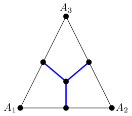
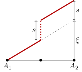
Figure 1: Sketch of the construction in Proposition 4.1 in the $2$d case. Left: decomposition of the triangle. The blue lines represent the jump set of $v$. Right: profile along a single edge. The parameter $s$ denotes the jump in the middle, the parameter $\xi$ the rest of the height change, which corresponds to the uniform slope in the rest.

Proposition 4.1.

Let $A_{1},\dots,A_{n+1}\in\mathbb{R}^{n}$ be such that $T:=\mathrm{conv}(\{A_{1},\dots,A_{n+1}\})$ has positive measure. There is a decomposition of $T$ into $n+1$ closed polyhedra $T_{1},\dots,T_{n+1}$ with disjoint interior such that the following holds. Let $u_{1},\dots,u_{n+1}\in\mathbb{R}$, fix $s\in\mathbb{R}_{*}:=\mathbb{R}^{(n+1)^{2}}_{\mathrm{skw}}$, and define $\xi\in\mathbb{R}_{*}$ by $\xi_{ij}+s_{ij}=u_{j}-u_{i}$. Then there is $v:T\to\mathbb{R}$ affine in each $T_{j}\setminus\bigcup_{i\neq j}\partial T_{i}$ and such that

$$|\nabla v|\leq{C\frac{\mathrm{diam}(T)^{n-1}}{|T|}}|\xi|\,,\hskip 28.45274pt|[v]|\leq{3}|s|,$$ (4.3)

$$\mathcal{H}^{n-1}(J_{v}\cap T)\leq\mathcal{H}^{n-1}(\partial T),$$ (4.4)

and with

$$v(A_{i}+t(A_{j}-A_{i}))=u_{i}+t\xi_{ij}+s_{ij}\chi_{t>1/2}$$ (4.5)

for all ${i<j}\in\{1,\dots,n+1\}$, $t\in[0,1]$. The constant $C$ depends only on $n$. The function $v$ depends linearly on $\{u_{i}\}\cup\{s_{ij}\}$.

The function $v$ on a face of $T$ does not depend on the opposing vertex. Precisely, for any $k$, if $x\in\mathrm{conv}(\{A_{1},\dots,A_{n+1}\}\setminus\{A_{k}\})$ then $v(x)$ depends only on $A_{i}$, $u_{i}$ for $i\neq k$ and on $s_{ij}$ for $i,j\neq k$.

Proof.

We first observe that each point $x\in T$ can be uniquely represented as $x=\sum_{i=1}^{n+1}\lambda_{i}A_{i}$ for some $\lambda\in\Lambda:=\{\lambda\in[0,1]^{n+1}:\sum_{i=1}^{n+1}\lambda_{i}=1\}$. We define the polyhedra $T_{j}$ by

$$T_{j}:=\{\sum_{i}\lambda_{i}A_{i}:{\lambda\in\Lambda},\lambda_{j}\geq\lambda_{i}\text{ for }i\neq j\},$$ (4.6)

see Figure 1(left) (in the case that $T$ is regular, this amounts to the Voronoi decomposition of $T$). We remark that the condition $\lambda_{i}\leq\lambda_{j}=1-\sum_{k\neq j}\lambda_{k}$ for all $i\neq j$ is equivalent to

$$2\lambda_{i}\leq 1-\sum_{k\neq i,j}\lambda_{k}\quad\mbox{ for all }i\neq j\,,$$ (4.7)

so that

$$x\in T_{j}\Longleftrightarrow x=A_{j}+\sum_{i\neq j}\lambda_{i}(A_{i}-A_{j})\quad\lambda\in\Lambda\mbox{ as in \eqref{e:lambdai}}\,.$$

We define $v_{j}:T_{j}\to\mathbb{R}$ by

$$v_{j}(x):=\hat{v}_{j}(\mathbb{A}_{j}^{-1}{(x-A_{j})})\,,$$

where $\mathbb{A}_{j}$ is the matrix with columns given by $A_{i}-A_{j}$ for $i\neq j$, and $\hat{v}_{j}:\mathbb{R}^{n}\to\mathbb{R}$ is defined by

$$\hat{v}_{j}(\lambda_{1},\ldots,\lambda_{j-1},\lambda_{j+1},\ldots,\lambda_{n+1}):=u_{j}+\sum_{i\neq j}\lambda_{i}\xi_{ji}$$ (4.8)

so that $v_{j}(\sum_{i}\lambda_{i}A_{i})=u_{j}+\sum_{i\neq j}\lambda_{i}\xi_{ji}$. We define $v$ by setting

$$v:=v_{j}\text{ in }T_{j}{\setminus\bigcup_{i<j}T_{i}.}$$ (4.9)

Obviously $A_{j}\in T_{j}$ and $v(A_{j})=u_{j}$. Further, for any $j$ the function $v$ is affine in $T_{j}\setminus\bigcup_{i<j}\partial T_{i}$, with

$$\nabla v(x)=(\mathbb{A}_{j}^{-1})^{T}\nabla\hat{v}_{j}(\mathbb{A}_{j}^{-1}{(x-A_{j})})=(\mathbb{A}_{j}^{-1})^{T}(\xi_{ji})_{i\neq j}$$

for all $x$ inside $T_{j}$, and therefore

$$|\nabla v|\leq\|\mathbb{A}_{j}^{-1}\|_{op}{|(\xi_{ji})_{i\neq j}|}\quad\mbox{ on }T_{j}$$

from which we infer that

$$|\det\mathbb{A}_{j}||\nabla v|\leq\|{\mathrm{cof\,}}\mathbb{A}_{j}\|_{op}{|\xi|}\quad\mbox{ on }T_{j}\,.$$

By definition of $\mathbb{A}_{j}$, it holds $|\det\mathbb{A}_{j}|=n!|T|$. As a cofactor is a homogeneous polynomial of degree $n-1$, one obtains $\|{\mathrm{cof\,}}\mathbb{A}_{j}\|_{op}\leq C\mathrm{diam}(T)^{n-1}$, for some dimensional constant $C<\infty$. This proves the first bound in (4.3).

To conclude that $v\in SBV(T)$, with the claimed estimates, we note that since by construction $v$ is affine on each $T_{j}$, it jumps only on the points $x=\sum_{i}\lambda_{i}A_{i}\in\partial T_{j}\cap\partial T_{k}$ for some $j\neq k$. Necessarily $\lambda_{j}=\lambda_{k}$, and the conditions $\xi_{ij}+s_{ij}=u_{j}-u_{i}$, $\sum_{i}\lambda_{i}=1$ with $\lambda_{i}\in[0,1]$, the antisymmetry of $\xi$, and the compatibility condition in (4.1) imply that

$$\begin{split}(v_{j}-v_{k})(\sum_{i}\lambda_{i}A_{i})&=u_{j}-u_{k}+\lambda_{k}\xi_{jk}-\lambda_{j}\xi_{kj}+\sum_{i\not\in\{j,k\}}\lambda_{i}(\xi_{ji}-\xi_{ki})\\ &=\xi_{kj}+s_{kj}-(\lambda_{k}+\lambda_{j})\xi_{kj}+\sum_{i\not\in\{j,k\}}\lambda_{i}(\xi_{ji}+\xi_{ik})\\ &=s_{kj}+\sum_{i\not\in\{j,k\}}\lambda_{i}(\xi_{kj}+\xi_{ji}+\xi_{ik})\\ &=s_{kj}-\sum_{i\not\in\{j,k\}}\lambda_{i}(s_{kj}+s_{ji}+s_{ik})\\ &{=(\lambda_{j}+\lambda_{k})s_{kj}-\sum_{i\not\in\{j,k\}}\lambda_{i}(s_{ji}+s_{ik}).}\end{split}$$ (4.10)

Therefore $v\in SBV(T)$ with $|[{v}]|\leq{3}|s|$ and

$$\mathcal{H}^{n-1}(J_{v})\leq\sum_{i\neq j}\mathcal{H}^{n-1}(\partial T_{i}\cap\partial T_{j})\leq\mathcal{H}^{n-1}(\partial T)\,.$$ (4.11)

The last inequality is proven in (4.19) below. This concludes the proof of (4.3) and (4.4). Condition (4.5) follows directly from the definition above.

By construction, it is clear that $v$ does not depend on the vertex $A_{k}$ on the opposing face $F_{k}$, since on $F_{k}$ we have $\lambda_{k}=0$ and $F_{k}\cap T_{k}=\emptyset$.

It remains to prove the geometric inequality that was used in the last step of (4.11). By Fubini’s theorem one easily checks the following: Consider a set $\alpha$ of $k+1$ points in $\mathbb{R}^{n}$, $0\leq k<n$. Then for any $x\in\mathbb{R}^{n}$ one has

$$\mathcal{H}^{k+1}(\mathrm{conv}(\alpha\cup\{x\}))=\frac{1}{k+1}\mathcal{H}^{k}(\mathrm{conv}(\alpha))\cdot\mathrm{dist}(x,\mathrm{\text{aff-span}}(\alpha)),$$ (4.12)

where $\mathrm{\text{aff-span}}(\alpha)$ is the smallest affine space that contains $\alpha$ (if $k=0$ then $\mathrm{conv}(\alpha)=\mathrm{\text{aff-span}}(\alpha)=\alpha$ and $\mathcal{H}^{0}(\mathrm{conv}(\alpha))=1$).

Fix now $i\neq j\in\{1,\dots,n+1\}$, and consider $\partial T_{i}\cap\partial T_{j}$. Then

$$\begin{split}\partial T_{i}\cap\partial T_{j}=&\{\sum_{p=1}^{n+1}\lambda_{p}A_{p}:\lambda\in\Lambda,\lambda_{i}=\lambda_{j}=\max_{p}\lambda_{p}\}\\ =&\{2\lambda_{i}\frac{A_{i}+A_{j}}{2}+\sum_{p\neq\{i,j\}}\lambda_{p}A_{p}:\lambda\in\Lambda,\lambda_{i}=\lambda_{j}=\max_{p}\lambda_{p}\}\\ \subseteq&\{\sum_{p=1}^{n}\lambda^{*}_{p}A_{p}^{*}:\lambda^{*}\in\Lambda^{*},\lambda^{*}_{1}=\max_{p}\lambda^{*}_{p}\},\end{split}$$ (4.13)

where $\Lambda^{*}:=\{\lambda^{*}\in[0,1]^{n}:\sum_{p=1}^{n}\lambda^{*}_{p}=1\}$, $A_{1}^{*}:=\frac{A_{i}+A_{j}}{2}$ and $\{A_{p}^{*}\}_{p=2,\dots,n}$ is any relabeling of the $n-1$ points in $\alpha_{ij}:=\{A_{1},\dots,A_{n+1}\}\setminus\{A_{i},A_{j}\}$ (the inclusion in the last step follows from the fact that $\lambda_{1}^{*}=2\lambda_{i}\geq{2}\lambda_{p}^{*}$ for all $p>1$). By symmetry, all $n$ sets $\{\lambda^{*}\in\Lambda^{*}:\lambda^{*}_{i}=\max_{p}\lambda^{*}_{p}\}$ have the same area, and as they are disjoint up to $\mathcal{H}^{n-1}$-dimensional null sets we obtain

$$\mathcal{H}^{n-1}(\partial T_{i}\cap\partial T_{j})\leq\frac{1}{n}\mathcal{H}^{n-1}\big{(}\mathrm{conv}\{A_{p}^{*}\}\big{)}=\frac{1}{n}\mathcal{H}^{n-1}\Big{(}\mathrm{conv}\big{(}\alpha_{ij}\cup\{\frac{A_{i}+A_{j}}{2}\}\big{)}\Big{)}$$ (4.14)

so that (4.12) gives

$$\mathcal{H}^{n-1}(\partial T_{i}\cap\partial T_{j})\leq\frac{1}{n(n-1)}\mathcal{H}^{n-2}(\mathrm{conv}(\alpha_{ij}))\cdot\mathrm{dist}\Big{(}\frac{A_{i}+A_{j}}{2},\mathrm{\text{aff-span}}(\alpha_{ij})\Big{)}.$$ (4.15)

By convexity

$$\mathrm{dist}\Big{(}\frac{A_{i}+A_{j}}{2},\mathrm{\text{aff-span}}(\alpha_{ij})\Big{)}\leq\frac{1}{2}\mathrm{dist}(A_{i},\mathrm{\text{aff-span}}(\alpha_{ij}))+\frac{1}{2}\mathrm{dist}(A_{j},\mathrm{\text{aff-span}}(\alpha_{ij}))\,.$$ (4.16)

Let $F_{i}:=\mathrm{conv}(\{A_{1},\dots,A_{n+1}\}\setminus\{A_{i}\})=\mathrm{conv}(\alpha_{ij}\cup\{A_{j}\})$ be the face opposite to the vertex $A_{i}$. By (4.12),

$$\mathcal{H}^{n-1}(F_{i})=\frac{1}{n-1}\mathcal{H}^{n-2}(\mathrm{conv}(\alpha_{ij}))\cdot\mathrm{dist}(A_{j},\mathrm{\text{aff-span}}(\alpha_{ij})).$$ (4.17)

Combining (4.15), (4.16) and (4.17) gives

$$\mathcal{H}^{n-1}(\partial T_{i}\cap\partial T_{j})\leq\frac{1}{2n}\mathcal{H}^{n-1}(F_{i})+\frac{1}{2n}\mathcal{H}^{n-1}(F_{j}).$$ (4.18)

We sum over all pairs $(i,j)$ with $i\neq j$ and obtain

$$\sum_{{i\neq j}}\mathcal{H}^{n-1}(\partial T_{i}\cap\partial T_{j})\leq\sum_{i=1}^{n+1}\sum_{j\neq i}\frac{1}{n}\mathcal{H}^{n-1}(F_{i})=\sum_{i=1}^{n+1}\mathcal{H}^{n-1}(F_{i})=\mathcal{H}^{n-1}(\partial T)$$ (4.19)

which concludes the proof. ∎

4.2 Projection on piecewise affine functions

In this section, we use Proposition 4.1 to construct a good piecewise affine interpolation of any vectorial function $u\in SBV_{\mathrm{loc}}(\mathbb{R}^{n};\mathbb{R}^{m})$ over a suitable partition of $\mathbb{R}^{n}$ in simplexes. First, Lemma 4.2 states the general properties of the chosen partition. Proposition 4.1 then can be applied componentwise in each simplex of a suitable shift of the partition. The resulting interpolation can be interpreted as a projection of $u$ over piecewise affine functions and enjoys good energy estimates, see Proposition 4.3.

Lemma 4.2.

For any $n\geq 1$ there is a countable set of simplexes $\mathcal{T}_{0}\subseteq\mathcal{P}(\mathbb{R}^{n})$ such that, denoting by $\mathrm{Vert}(\tau_{0})$ the set of vertices of $\tau_{0}\in\mathcal{T}_{0}$, one has:

1. $\#\mathrm{Vert}(\tau_{0})=n+1$; $|\tau_{0}|>0$ for all $\tau_{0}\in\mathcal{T}_{0}$;

2. $\tau_{0}\cap\tau^{\prime}_{0}=\mathrm{conv}(\mathrm{Vert}(\tau_{0})\cap\mathrm{Vert}(\tau_{0}^{\prime}))$, in particular $|\tau_{0}\cap\tau^{\prime}_{0}|=0$ if $\tau_{0}\neq\tau^{\prime}_{0}$;

3. $\bigcup_{\tau_{0}\in\mathcal{T}_{0}}\tau_{0}=\mathbb{R}^{n}$;

4. For any $\tau_{0}\in\mathcal{T}_{0}$ there is $z\in\mathbb{Z}^{n}$ such that $\mathrm{Vert}(\tau_{0})\subseteq\{z+\sum_{i}\lambda_{i}e_{i}:\,\lambda_{i}\in\{0,1\},\,i\in\{1,\ldots,n\}\}$, with the $e_{i}$’s the canonical basis vectors;

5. If $\tau_{0}\in\mathcal{T}_{0}$, then $\tau_{0}+2e_{i}\in\mathcal{T}_{0}$, with $e_{i}$ any of the canonical basis vectors.

We recall that $\mathrm{conv}(\emptyset)=\emptyset$. Condition (i) and condition (ii) with $\tau_{0}=\tau^{\prime}_{0}$ imply that $\tau_{0}$ is a closed simplex. Condition (iv) implies that for all $\varepsilon>0$, the rescaled simplex $\varepsilon{\tau_{0}}$ has diameter at most $\varepsilon\sqrt{n}$, and together with condition (i) that its volume is at least $\varepsilon^{n}/n!$ (indeed, it is $1/n!$ times the determinant of a matrix with entries in $\{-\varepsilon,0,\varepsilon\}$). The last two imply that this is a refinement of the natural subdivision of $\mathbb{R}^{n}$ into unitary cubes, with period $[0,2]^{n}$.

Proof.

This can be obtained taking any partition, as for example the Freudenthal partition, of $[0,1]^{n}$, reflecting this along the coordinate axes to obtain a partition of $[-1,1]^{n}$, and then extending periodically. ∎

In the rest of this section we define for any $\varepsilon>0$ and $\zeta\in B_{\varepsilon}$ a projection $\Pi_{\varepsilon,\zeta}$ on the space of functions that are affine on each polyhedron in a refinement of $\zeta+\varepsilon\mathcal{T}_{0}$. The projection will be used on functions $u\in SBV(\mathbb{R}^{n};\mathbb{R}^{m})$. As it depends on point values, we shall only obtain a well-defined result for values of the translation $\zeta$ outside a null set. The null set, however, depends on $u$. To avoid this, the precise definition is given not on equivalence classes but on functions from $\mathbb{R}^{n}$ to $\mathbb{R}^{m}$. In order to understand the key properties, it is useful to consider first the action of $\Pi_{\varepsilon,\zeta}$ on elements of $SBV(\mathbb{R}^{n};\mathbb{R}^{m})$ (or, equivalently, $SBV_{\mathrm{loc}}(\mathbb{R}^{n};\mathbb{R}^{m})$, since $\Pi_{\varepsilon,\zeta}$ is local).

Let $u\in SBV(\mathbb{R}^{n};\mathbb{R}^{m})$. For any couple of vertices $a\neq b\in\mathrm{Vert}(\tau)$ of a simplex $\tau\in\zeta+\varepsilon\mathcal{T}_{0}$, we consider the slice $u_{a}^{b-a}(t):=u(a+t(b-a))$. For $\mathcal{L}^{2n}$-almost every pair $(a,b)$ we have $u_{a}^{b-a}\in SBV({\mathbb{R}};\mathbb{R}^{m})$ with

$$u(b)-u(a)=\int_{0}^{1}(u_{a}^{b-a})^{\prime}(t)dt+\sum_{t\in(0,1)\cap J_{u_{a}^{b-a}}}[u_{a}^{b-a}](t)$$ (4.20)

with

$$(u_{a}^{b-a})^{\prime}(t)=\nabla u(a+t(b-a))(b-a)$$

and

$$[u_{a}^{b-a}](t)=[u](a+t(b-a))\mathrm{sgn}(\nu_{a+t(b-a)}\cdot(b-a))$$

(see [AFP00, Sect. 3.11] or [Bra98, Th. 4.1(a)]). The parameters $s$ and $\xi$ entering the piecewise affine construction in Proposition 4.1 are then defined from the two components of (4.20). Precisely, we define the jump over an edge $[a,b]$ by

$$s_{[a,b]}:=\sum_{t\in(0,1){\cap J_{u_{a}^{b-a}}}}[u](a+t(b-a)){\mathrm{sgn}(\nu_{a+t(b-a)}\cdot(b-a))}$$ (4.21)

(setting it to zero if the sum does not converge or is not defined) and correspondingly the integral of the absolutely continuous part of the gradient by

$$\xi_{[a,b]}:=u(b)-u(a)-s_{[a,b]}.$$ (4.22)

For $\mathcal{L}^{2n}$-almost all pairs $(a,b)$

$$\xi_{[a,b]}=\int_{0}^{1}\nabla u(a+t(b-a))(b-a)dt.$$ (4.23)

By monotonicity and subadditivity of $g_{0}$,

$$g_{0}({|s_{[a,b]}|})\leq\sum_{t\in(0,1){\cap J_{u_{a}^{b-a}}}}{g_{0}(|[u](a+t(b-a))|)}\,.$$ (4.24)

Similarly, for $\mathcal{L}^{2n}$-almost all pairs $(a,b)$, using (4.23) and Jensen’s inequality,

$${\left|\frac{\xi_{[a,b]}}{|b-a|}\right|^{p}\leq\int_{0}^{1}|\nabla u(a+t(b-a))|^{p}dt.}$$ (4.25)

In Proposition 4.3 we will turn both estimates (4.24) and (4.25) into estimates relating the energy over shifts of the segment, averaged over all possible shifts of size less than $\varepsilon$, and integrals over $J_{u}$ and $\Omega$, respectively.

Proposition 4.3.

There is a locally finite subdivision of $\mathbb{R}^{n}$ into countably many essentially disjoint polyhedra, $\mathcal{T}^{*}_{0}$, finer than $\mathcal{T}_{0}$ and with the same periodicity, and $C>0$ such that, for any $\varepsilon>0$ and $\zeta\in B_{\varepsilon}$, to any function $f:\mathbb{R}^{n}\to\mathbb{R}^{m}$ one can associate a function $\Pi_{\varepsilon,\zeta}f:\mathbb{R}^{n}\to\mathbb{R}^{m}$, affine in the interior of each element of $\mathcal{T}_{\varepsilon,\zeta}^{*}:=\zeta+\varepsilon\mathcal{T}_{0}^{*}$, so that the following holds:

1. If either ${\tau_{0}}\in\mathcal{T}_{0}$ or ${\tau_{0}}\in\mathcal{T}^{*}_{0}$ then $\mathrm{diam}({\tau_{0}})\leq\sqrt{n}$ and $|{\tau_{0}}|\geq 1/C$;

2. $\Pi_{\varepsilon,\zeta}$ is a projection, in the sense that $\Pi_{\varepsilon,\zeta}\Pi_{\varepsilon,\zeta}f=\Pi_{\varepsilon,\zeta}f$ for all $f$, and it commutes with translations, in the sense that $\Pi_{\varepsilon,\zeta}[f(\cdot-\zeta)]=[\Pi_{\varepsilon,0}f](\cdot-\zeta)$;

3. One has $\Pi_{\varepsilon,\zeta}{f}\in SBV_{\mathrm{loc}}(\mathbb{R}^{n};\mathbb{R}^{m})$ and, with $\mathcal{T}_{\varepsilon,\zeta}:=\zeta+\varepsilon\mathcal{T}_{0}$,

   $$|D\Pi_{\varepsilon,\zeta}{f}|(\bigcup_{\tau\in\mathcal{T}_{\varepsilon,\zeta}}\partial\tau)=0.$$ (4.26)

   If $u\in SBV_{\mathrm{loc}}(\mathbb{R}^{n};\mathbb{R}^{m})$, then for $\mathcal{L}^{n}$-almost every $\zeta\in B_{\varepsilon}$ one has

   $$\mathcal{H}^{n-1}(J_{u}\cap\bigcup_{\tau\in\mathcal{T}_{\varepsilon,\zeta}}\partial\tau)=0.$$

4. The function $\Pi_{\varepsilon,\zeta}{f}$ on a set $\omega$ depends only on the value of ${f}$ on the set $(\omega)_{\varepsilon\sqrt{n}}$.

5. If ${A}:\mathbb{R}^{n}\to\mathbb{R}^{m}$ is affine and $\lambda\in\mathbb{R}$, then for any function ${f}$ one has $\Pi_{\varepsilon,\zeta}(\lambda{f}+{A})=\lambda(\Pi_{\varepsilon,\zeta}{f})+{A}$; if $u,v\in SBV_{\mathrm{loc}}(\mathbb{R}^{n};\mathbb{R}^{m})$ then for almost every $\zeta\in B_{\varepsilon}$ one has $\Pi_{\varepsilon,\zeta}(u+v)=\Pi_{\varepsilon,\zeta}u+\Pi_{\varepsilon,\zeta}v$;

6. For any $\eta\in\mathbb{R}^{m\times n}$ and $\tau_{0}\in\mathcal{T}_{0}$, one has for any $u\in SBV_{\mathrm{loc}}(\mathbb{R}^{n};\mathbb{R}^{m})$ that

   $$\fint_{B_{\varepsilon}}\Big{(}\int_{\zeta+\varepsilon{\tau_{0}}}|\nabla\Pi_{\varepsilon,\zeta}u-\eta|^{p}dx\Big{)}d\zeta\leq C\int_{{{(\varepsilon\tau_{0})_{{c_{*}}\varepsilon}}}}|\nabla u-\eta|^{p}dx,$$ (4.27)

   $$\fint_{B_{\varepsilon}}{\Big{(}}\int_{J_{\Pi_{\varepsilon,\zeta}u}\cap(\zeta+\varepsilon\tau_{0})}g_{0}(|[\Pi_{\varepsilon,\zeta}u]|)d\mathcal{H}^{n-1}{\Big{)}}d\zeta\leq C\int_{J_{u}\cap{(\varepsilon\tau_{0})_{{c_{*}}\varepsilon}}}g_{0}(|[u]|)d\mathcal{H}^{n-1},$$ (4.28)

   $$\fint_{B_{\varepsilon}}\mathcal{H}^{n-1}(J_{\Pi_{\varepsilon,\zeta}u}\cap(\zeta+\varepsilon\tau_{0}))d\zeta\leq C\mathcal{H}^{n-1}(J_{u}\cap{(\varepsilon\tau_{0})_{{c_{*}}\varepsilon}}),$$ (4.29)

   $$\fint_{B_{\varepsilon}} \Big{(}\int_{\zeta+\varepsilon\tau_{0}}|\Pi_{\varepsilon,\zeta}u-u|dx\Big{)}d\zeta\leq C\varepsilon|Du|({(\varepsilon\tau_{0})_{{c_{*}}\varepsilon}}),$$ (4.30)

   and, for every $n-1$-rectifiable set $\Sigma$,

   $$\fint_{B_{\varepsilon}}{\Big{(}}\int_{\Sigma}|\Pi_{\varepsilon,\zeta}u|d\mathcal{H}^{n-1}{\Big{)}}d\zeta\leq\frac{Ck_{\Sigma}}{\varepsilon}\|u\|_{L^{1}((\Sigma)_{{c_{*}}\varepsilon})}+{Ck_{\Sigma}}|Du|((\Sigma)_{2{c_{*}}\varepsilon}),$$ (4.31)

   where

   $$k_{\Sigma}:=\sup_{r>0,x\in\mathbb{R}^{n}}\frac{\mathcal{H}^{n-1}(\Sigma\cap B_{r}(x))}{r^{n-1}}.$$ (4.32)

   Here ${c_{*}}\in[1+\sqrt{n},\infty)$ is a constant that depends only on $n$; $C$ may depend on $n$, $m$, $p$.

7. If $u\in SBV_{\mathrm{loc}}(\mathbb{R}^{n};\mathbb{R}^{m})$ and $\nabla u=0$ $\mathcal{L}^{n}$-almost everywhere then for almost every $\zeta\in B_{\varepsilon}$ one has $\nabla\Pi_{\varepsilon,\zeta}u=0$ $\mathcal{L}^{n}$-almost everywhere. In particular, if $u=\chi_{E}$ for some set $E$ then there is a countable union of polygons $F_{\varepsilon,\zeta}$ such that $\Pi_{\varepsilon,\zeta}u=\chi_{F_{\varepsilon,\zeta}}$. If $\mathcal{H}^{n-1}(J_{u})=0$ then for almost every $\zeta\in B_{\varepsilon}$ one has $\mathcal{H}^{n-1}(J_{\Pi_{\varepsilon,\zeta}u})=0$.

Condition (4.27) easily implies that for any Borel set $\omega\subset\mathbb{R}^{n}$ and any $\eta$

$$\fint_{B_{\varepsilon}}\Big{(}\int_{\omega}|\nabla\Pi_{\varepsilon,\zeta}u-\eta|^{p}dx\Big{)}d\zeta\leq C\int_{{{(\omega)_{2{c_{*}}\varepsilon}}}}|\nabla u-\eta|^{p}dx.$$ (4.33)

Indeed, it suffices to sum (4.27) over all $\tau_{0}\in\mathcal{T}_{0}$ such that there is $\zeta\in B_{\varepsilon}$ with $(\zeta+\varepsilon\tau_{0})\cap\omega\neq\emptyset$, which implies $\varepsilon\tau_{0}\subseteq(\omega)_{(1+\sqrt{n})\varepsilon}$. Analogous observations hold for (4.28), (4.29) and (4.30).

We remark that (4.31) fails if we remove the derivative term in the right-hand side. Consider for example the sequence $u_{j}(x):=\frac{1}{j}\langle jx_{1}\rangle$, where $\langle x\rangle:=x-\lfloor x\rfloor$ denotes the fractional part of $x\in\mathbb{R}$, which converges uniformly to $0$ as $j\to\infty$. As $\nabla u_{j}e_{1}=1$ almost everywhere, for any $\varepsilon$ and $\zeta$ we have $\partial_{1}\Pi_{\varepsilon,\zeta}u_{j}=1$ almost everywhere, and since $\Pi_{\varepsilon,\zeta}u_{j}$ is piecewise affine on a scale $\varepsilon$ we obtain $\|\Pi_{\varepsilon,\zeta}u_{j}\|_{L^{\infty}}\geq\frac{1}{2}\varepsilon$, which does not depend on $j$. Similarly, one cannot estimate $\Pi_{\varepsilon,\zeta}u$ in $L^{1}$ only in terms of the $L^{1}$ norm of $u$.

Proof.

The grid $\mathcal{T}_{0}^{*}$ is defined decomposing each simplex $\tau_{0}\in\mathcal{T}_{0}$ as in Proposition 4.1. The projection $\Pi_{\varepsilon,\zeta}{f}$ is defined by application of the construction in Proposition 4.1 componentwise in each simplex $\tau\in\mathcal{T}_{\varepsilon,\zeta}=\zeta+\varepsilon\mathcal{T}_{0}$.

Precisely, let $\tau=\zeta+\varepsilon\tau_{0}$, for some $\tau_{0}\in\mathcal{T}_{0}$, and let $\{w_{1},\dots,w_{n+1}\}:=\mathrm{Vert}(\tau)$ be its vertices. In order to define the cumulated jump over the edge $[w_{i},w_{j}]$ we consider the slice $v^{{f}}_{ij}(t):={f}(w_{i}+t(w_{j}-w_{i}))$, for $t\in[0,1]$. If $v^{{f}}_{ij}\in SBV((0,1);\mathbb{R}^{m})$ then we set

$${s_{ij}^{{f}}}:=\sum_{t\in(0,1)\cap J_{v^{{f}}_{ij}}}[v^{{f}}_{ij}](t),$$ (4.34)

otherwise we set ${s_{ij}^{{f}}}:=0$. The function $\Pi_{\varepsilon,\zeta}{{f}}$ is then defined in $\tau$ using Proposition 4.1 componentwise. As discussed above, if ${f}=u\in SBV_{\mathrm{loc}}(\mathbb{R}^{n};\mathbb{R}^{m})$ then for almost every choice of $\zeta$ one has that ${v_{ij}^{u}}\in SBV((0,1);\mathbb{R}^{m})$ for all choices of $\tau_{0}$ and of $i,j$.

(i): The upper bound on the diameter follows from Lemma 4.2 and the fact that $\mathcal{T}_{0}^{*}$ is a refinement of $\mathcal{T}_{0}$. The lower bound on the volume follows from the fact that both grids are locally finite and periodic.

(ii): Assume for simplicity that $f$ is scalar. For any $\tau$ and $w_{1},\dots,w_{n+1}$ as above, one easily obtains that $(\Pi_{\varepsilon,\zeta}f)(w_{i})=f(w_{i})$. Let $s_{ij}^{f}$ be defined as in (4.34). By (4.5) the function $v_{ij}^{\Pi_{\varepsilon,\zeta}f}$ has a unique jump point in $(0,1)$, which is located at $1/2$, and the amplitude of the jump is exactly $s_{ij}^{f}$. Therefore $s_{ij}^{\Pi_{\varepsilon,\zeta}f}=s_{ij}^{f}$ and $\Pi_{\varepsilon,\zeta}$ is a projection. The relation to translations follows observing that for any $\tau_{0}\in\mathcal{T}_{0}$ the vertices of ${\zeta+\varepsilon\tau_{0}}$ are translated with respect to the vertices of ${\varepsilon\tau_{0}}$ by $\zeta$.

(iii): Let $\tau\neq\tau^{\prime}\in\mathcal{T}_{\varepsilon,\zeta}$ be such that ${\mathcal{H}^{n-1}(\partial\tau\cap\partial\tau^{\prime})>0}$, so that by Lemma 4.2(ii) $\partial\tau\cap\partial\tau^{\prime}=\mathrm{conv}(\mathrm{Vert}(\tau)\cap\mathrm{Vert}(\tau^{\prime}))$. Proposition 4.1 implies that $\Pi_{\varepsilon,\zeta}{f}|_{\partial\tau\cap\partial\tau^{\prime}}$ only depends on the in-plane vertices $\mathrm{Vert}(\tau)\cap\mathrm{Vert}(\tau^{\prime})$, on the values of ${f}$ on such vertices, and on the jumps $s_{\sigma}$ on the in-plane edges $\sigma\subset\partial\tau\cap\partial\tau^{\prime}$. Hence $|D\Pi_{\varepsilon,\zeta}{f}|(\bigcup_{\tau\in\mathcal{T}_{\varepsilon,\zeta}}\partial\tau)=0$. The second condition follows from the fact that $\mathcal{H}^{n-1}\mathop{\hbox{\vrule height=7.0pt,width=0.5pt,depth=0.0pt\vrule height=0.5pt,width=6.0pt,depth=0.0pt}}\nolimits{J_{u}}$ is $\sigma$-finite.

(iv): Given a set $\omega\subset\mathbb{R}^{n}$, the function $\Pi_{\varepsilon,\zeta}{f}|_{\omega}$ only depends on the values of ${f}$ on the vertices of the simplexes intersecting $\omega$. Since their diameter is by construction not greater than $\varepsilon\sqrt{n}$, $\Pi_{\varepsilon,\zeta}{f}|_{\omega}$ only depends on the value of ${f}$ on the neighborhood $(\omega)_{\varepsilon\sqrt{n}}$.

(v): It follows from the fact that the function constructed in Proposition 4.1 depends linearly on the prescribed values on the vertices $u_{i}$ and jumps $s_{ij}$.

(vi): By (v), it suffices to prove the first bound in the case $\eta=0$. Let ${\tau_{0}}\in\mathcal{T}_{0}$, and $\{w_{1},\dots,w_{n+1}\}=\mathrm{Vert}(\varepsilon\tau_{0})$. For any $\zeta\in B_{\varepsilon}$, by the uniform estimate in (4.3) we have

$${\int_{\zeta+\varepsilon{\tau_{0}}}{|\nabla\Pi_{\varepsilon,\zeta}u|^{p}}dx\leq C\varepsilon^{n}\sum_{i,j}\Big{|}\frac{\xi_{\zeta+[w_{i},w_{j}]}}{|w_{i}-w_{j}|}\Big{|}^{p}.}$$ (4.35)

Next, we claim that for all $i,j$

$$\int_{B_{\varepsilon}}\left|\frac{\xi_{\zeta+[w_{i},w_{j}]}}{{|w_{i}-w_{j}|}}\right|^{p}d\zeta\leq\int_{{B_{(1+{\sqrt{n}})\varepsilon}(w_{i})}}|\nabla u|^{p}dx.$$ (4.36)

Indeed, starting from (4.25) and integrating over all translations $\zeta\in B_{\varepsilon}$ we get, setting $\ell:=w_{j}-w_{i}$,

$$\begin{split}{\int_{B_{\varepsilon}}\left|\frac{\xi_{\zeta+[w_{i},w_{j}]}}{{|\ell|}}\right|^{p}}d\zeta\leq&\int_{B_{\varepsilon}}\int_{0}^{1}|\nabla u(\zeta+{w_{i}+t\ell})|^{p}dtd\zeta\\ =&\int_{0}^{1}\int_{B_{\varepsilon}({w_{i}}+t\ell)}|\nabla u(x)|^{p}dxdt\leq\int_{B_{{(1+\sqrt{n})}\varepsilon}({w_{i}})}|\nabla u|^{p}dx\end{split}$$

since $|\ell|=|w_{i}-w_{j}|\leq\varepsilon\sqrt{n}$. Therefore, from (4.35) and (4.36) we conclude

$$\fint_{B_{\varepsilon}} \Big{(}\int_{\zeta+\varepsilon\tau_{0}}{|\nabla\Pi_{\varepsilon,\zeta}u|^{p}}dx\Big{)}d\zeta$$

$$\leq C\sum_{i}\int_{B_{{({1+\sqrt{n}})}\varepsilon}({w_{i}})}|\nabla u|^{p}dx\leq C\int_{{(\varepsilon\tau_{0})_{(1+\sqrt{n})\varepsilon}}}|\nabla u|^{p}dx,$$

which concludes the proof of (4.27).

Analogously, using (iii), (4.3), and (4.4), we get

$$\int_{J_{\Pi_{\varepsilon,\zeta}u}\cap(\zeta+\varepsilon{\tau_{0}})}g_{0}({|[\Pi_{\varepsilon,\zeta}u]|})d\mathcal{H}^{n-1}\leq C\varepsilon^{n-1}\sum_{i,j}g_{0}({|s_{\zeta+{[w_{i},w_{j}]}}|}),$$ (4.37)

by monotonicity and subadditivity of $g_{0}$, where as before the $w_{i}$ are the vertices of ${\varepsilon\tau_{0}}$. We claim that

$$\int_{B_{\varepsilon}}{g_{0}({|s_{\zeta+{[w_{i},w_{j}]}}|})}d\zeta\leq C\varepsilon\int_{B_{{(2+{\sqrt{n}})}\varepsilon}({w_{i}})\cap J_{u}}{g_{0}(|[u]|)}d\mathcal{H}^{{n-1}}\,.$$ (4.38)

Indeed, we start from (4.24), integrate over translations, and separate the component $\zeta_{\ell}$ along $\ell$ from the orthogonal ones, which we denote by $\zeta^{\prime}$, so that $\zeta=\zeta^{\prime}+{\zeta_{\ell}}\ell/|\ell|$. Using the Coarea formula we estimate as follows

$$\begin{split}{\int_{B_{\varepsilon}}g_{0}({|s_{\zeta+{[w_{i},w_{j}]}}|})d\zeta}&\leq\int_{B_{\varepsilon}}\sum_{t\in(0,1)}{g_{0}(|[u](\zeta+{w_{i}}+t\ell)|)}d\zeta\\ &\leq\int_{-\varepsilon}^{\varepsilon}\int_{B^{\prime}_{\varepsilon}}\sum_{t\in(0,1)}{g_{0}(|[u]({\zeta^{\prime}}+{w_{i}}+t\ell+\zeta_{\ell}\frac{\ell}{|\ell|})|)}d\zeta^{\prime}d{\zeta_{\ell}}\\ &\leq 2\varepsilon\int_{B^{\prime}_{\varepsilon}}\sum_{t\in(-\varepsilon,\varepsilon(1+{\sqrt{n}}))}{g_{0}(|[u](\zeta^{\prime}+{w_{i}}+t\frac{\ell}{|\ell|})|)}d\zeta^{\prime}\\ &\leq 2\varepsilon\int_{J_{u}\cap B_{{{(2+\sqrt{n}})}\varepsilon}({w_{i}})}{g_{0}(|[u]|)}\,\Big{|}{\nu_{u}}\cdot\frac{\ell}{|\ell|}\Big{|}d\mathcal{H}^{n-1}{.}\end{split}$$ (4.39)

Clearly, (4.38) easily follows from (4.39).

Hence, by (4.37) and (4.38)

$$\fint_{B_{\varepsilon}}\int_{J_{\Pi_{\varepsilon,\zeta}u}\cap(\zeta+\varepsilon{\tau_{0}})}{g_{0}(|[\Pi_{\varepsilon,\zeta}u]|)}d\mathcal{H}^{n-1}d\zeta\leq C\int_{J_{u}\cap{(\varepsilon\tau_{0})_{{(2+\sqrt{n})}\varepsilon}}}g_{0}(|[u]|)d\mathcal{H}^{n-1}$$ (4.40)

which concludes the proof of (4.28).

The proof of (4.29) is similar. Let $g_{1}:[0,\infty)\to[0,\infty)$ be defined by $g_{1}(0)=0$, $g_{1}(s)=1$ for $s\neq 0$. The derivation of (4.37) above uses only (iii), (4.3), (4.4), and the fact that $g_{0}$ is nondecreasing and subadditive, and $g_{1}$ has the same properties. By (4.34), $s_{ij}^{u}=0$ if $v^{u}_{ij}$ does not jump on $[0,1]$, thus we obtain instead of (4.37) the estimate

$$\int_{J_{\Pi_{\varepsilon,\zeta}u}\cap(\zeta+\varepsilon{\tau_{0}})}g_{1}({|[\Pi_{\varepsilon,\zeta}u]|})d\mathcal{H}^{n-1}\leq C\varepsilon^{n-1}\sum_{i,j}g_{1}({|s_{\zeta+{[w_{i},w_{j}]}}|}).$$ (4.41)

The rest of the computation leading to (4.40) is unchanged. This proves (4.29).

Next, we estimate the $L^{1}$ distance of $u$ from $\Pi_{\varepsilon,\zeta}u$. By (4.3) for ${\tau_{0}}\in\mathcal{T}_{0}$ one has the pointwise estimate

$$\fint_{B_{\varepsilon}} \int_{\zeta+\varepsilon{\tau_{0}}}|\Pi_{\varepsilon,\zeta}u-u|dx\,d\zeta$$

$$\leq\fint_{B_{\varepsilon}}\int_{\zeta+\varepsilon{\tau_{0}}}\sum_{i}|u(\zeta+{w_{i}})-u(x)|dx\,d\zeta+C\varepsilon^{n}\fint_{B_{\varepsilon}}\sum_{i,j}|\xi_{\zeta+{[w_{i},w_{j}]}}|d\zeta.$$

We observe that for all choices of $i$, $\zeta$ and $x$ we have $x\in\zeta+\varepsilon\tau_{0}\subseteq{(\varepsilon\tau_{0})_{\varepsilon}}$ and $\zeta+w_{i}\in\zeta+\varepsilon\tau_{0}\subseteq{(\varepsilon\tau_{0})_{\varepsilon}}$. Therefore, each addend in the first term can be estimated using Poincaré’s inequality for $BV$ functions by

$$\fint_{B_{\varepsilon}}\int_{\zeta+\varepsilon{\tau_{0}}} |u(\zeta+{w_{i}})-u(x)|dx\,d\zeta\leq\frac{1}{|B_{\varepsilon}|}\int_{(\varepsilon\tau_{0})_{\varepsilon}}\int_{(\varepsilon\tau_{0})_{\varepsilon}}|u(y)-u(y^{\prime})|dydy^{\prime}$$

$$\leq {2}\frac{|{(\varepsilon\tau_{0})_{\varepsilon}}|}{|B_{\varepsilon}|}\int_{(\varepsilon\tau_{0})_{\varepsilon}}|u(y)-\bar{u}|dy\leq C\varepsilon|Du|{((\varepsilon\tau_{0})_{\varepsilon})},$$

where $\bar{u}$ denotes the average of $u$ in $(\varepsilon\tau_{0})_{\varepsilon}$. For the second one, we write using (4.36) with $p=1$

$$\varepsilon^{n}\fint_{B_{\varepsilon}}\sum_{i,j}|\xi_{\zeta+{[w_{i},w_{j}]}}|d\zeta\leq C\varepsilon\int_{(\varepsilon\tau_{0})_{C\varepsilon}}|\nabla u|dx.$$

Combining the two gives (4.30).

Finally, we prove (4.31): for any $\tau_{0}\in\mathcal{T}_{0}$ and $\zeta\in B_{\varepsilon}$, we have $\mathcal{H}^{n-1}(\Sigma\cap(\zeta+\varepsilon\tau_{0}))\leq Ck_{\Sigma}\varepsilon^{n-1}$. As the map $\Pi_{\varepsilon,\zeta}u$ is affine on each element of $\zeta+\varepsilon\mathcal{T}_{0}^{*}$, we have

$$\|\Pi_{\varepsilon,\zeta}u\|_{L^{\infty}(\zeta+\varepsilon\tau_{0})}\leq\frac{C}{\varepsilon^{n}}\|\Pi_{\varepsilon,\zeta}u\|_{L^{1}(\zeta+\varepsilon\tau_{0})}.$$ (4.42)

We sum over all $\tau_{0}$ such that $\zeta+\varepsilon\tau_{0}$ intersects $\Sigma$ and obtain

$$\int_{\Sigma}|\Pi_{\varepsilon,\zeta}u|d\mathcal{H}^{n-1}\leq\frac{Ck_{\Sigma}}{\varepsilon}\|\Pi_{\varepsilon,\zeta}u\|_{L^{1}((\Sigma)_{\sqrt{n}\varepsilon})}$$ (4.43)

for a.e. $\zeta\in B_{\varepsilon}$. Then we use (4.30) and a triangular inequality to conclude.

(vii): If $\nabla u=0$ $\mathcal{L}^{n}$-almost everywhere, then (4.27) with $\eta=0$ implies $\nabla\Pi_{\varepsilon,\zeta}u=0$ $\mathcal{L}^{n}$-almost everywhere for $\mathcal{L}^{n}$-almost every $\zeta$. If $u$ takes values in $\{0,1\}$, then for each application of Proposition 4.1 we have that $\xi_{ij}=0$, therefore the constructed function is piecewise constant and takes values in the set $\{u_{1},\dots,u_{n+1}\}\subseteq\{0,1\}$.

Finally, if $\mathcal{H}^{n-1}(J_{u})=0$ then necessarily $u\in{W^{1,1}_{\mathrm{loc}}}(\mathbb{R}^{n};\mathbb{R}^{m})$. In turn, the slices of $u$ are Sobolev functions for $\mathcal{L}^{n}$-almost every $\zeta\in B_{\varepsilon}$, so that $J_{\Pi_{\varepsilon,\zeta}u}=\emptyset$, in turn implying that $\Pi_{\varepsilon,\zeta}u$ is actually continuous and in ${W^{1,1}_{\mathrm{loc}}}(\mathbb{R}^{n};\mathbb{R}^{m})$ (alternatively, this follows also from (4.29)). ∎

4.3 Global construction

We are now ready to establish Theorem 1.1. The proof contains two different scales, denoted by $\delta$ and $\varepsilon$ in the following. The scale $\delta$ is the one at which the function $u$ has approximately regular jump and gradient, and is identified in Proposition 3.6. The second scale $\varepsilon\ll\delta$, used for the construction in Proposition 4.3, is the one on which we construct a piecewise affine approximation of $u$. This is achieved in each cube at scale $\delta$ by applying Proposition 4.3 to the extensions, obtained via Theorem 3.5, of $u$ itself restricted to domains separated by the regular part of its jump set. In turn, the regularization $L_{z}$ of the jump set $J_{u}$ will be separately approximated using piecewise affine elements in $\mathbb{R}^{n-1}$ using again the scale $\varepsilon$. Figure 3 shows a sketch of the construction, the different parts will become clear during the proof.

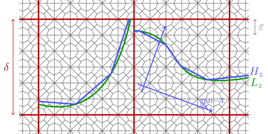
Figure 3: Sketch of the grids used in the proof of Theorem 1.1. The grid $(\mathcal{T}^{\prime},V^{\prime})$ is taken in $\mathbb{R}^{n-1}$, it is then rotated. Similarly, $H_{z}$ and $L_{z}$ are graphs (of $\psi_{z}$ and $\varphi_{z}$, respectively) in these rotated coordinates.

Proof of Theorem 1.1.

Let $u\in SBV(\Omega;\mathbb{R}^{m})$ and $\theta\in{(0,\frac{1}{2}]}$. To simplify the notation we work at fixed $\theta$, and in the end choose a sequence $\theta_{j}\to 0$. It is not restrictive to assume additionally that

$${t\leq g_{0}(t)\text{ for all }t\in[0,\infty)};$$ (4.44)

indeed, this follows by proving first the theorem with $g_{0}(t)+t$ in place of $g_{0}$ and then deducing the statement for $g_{0}$ as a by-product. By (2.2), for any $\lambda>0$ (fixed below, it will depend on $\theta$ and $\delta$ but not on $\varepsilon$ and $\delta^{\prime}$; $\lambda=\theta\delta$ will do) there is $C_{\lambda}\geq 1$ such that

$$g_{0}({t})\leq\lambda+C_{\lambda}{t}\text{ for all }{t\in[0,\infty)}.$$ (4.45)

This will be used to estimate terms of the form $g_{0}({|}[w]{|})$ on sets of finite $n-1$-dimensional measure in terms of the jump.

• Choice of the scale $\delta$ on which $u$ is regular and of the sets $A_{\delta}$, $A_{\delta}^{*}$.

  By Theorem 3.5 we can assume that $u\in SBV(\mathbb{R}^{n};\mathbb{R}^{m})$ with $|Du|(J_{u}\cap\partial\Omega)=0$,

  $$\int_{\Omega^{\prime}}|\nabla u|^{p}\,dx\leq\int_{\Omega}|\nabla u|^{p}\,dx+\theta\,,$$ (4.46)

  and

  $$\int_{\Omega^{\prime}\cap J_{u}}g_{0}(|[u]|)d\mathcal{H}^{n-1}\leq\int_{\Omega\cap J_{u}}g_{0}(|[u]|)d\mathcal{H}^{n-1}+\theta\,,$$ (4.47)

  for some bounded open set $\Omega^{\prime}$ with $\overline{\Omega}\subset\Omega^{\prime}$ and $|\Omega^{\prime}|\leq 2|\Omega|$. We choose $\delta_{0}\in(0,\theta]$ such that $3\delta_{0}\sqrt{n}\leq\mathrm{dist}(\Omega,\partial\Omega^{\prime})$ and

  $$\int_{(\partial\Omega)_{3\delta_{0}\sqrt{n}}}|\nabla u|^{p}dx+\mu_{u}((\partial\Omega)_{3\sqrt{n}\delta_{0}})\leq\theta,$$ (4.48)

  where $\mu_{u}:=g_{0}(|[u]|)\mathcal{H}^{n-1}\mathop{\hbox{\vrule height=7.0pt,width=0.5pt,depth=0.0pt\vrule height=0.5pt,width=6.0pt,depth=0.0pt}}\nolimits J_{u}$ as in (3.41). If $\mathcal{H}^{n-1}(J_{u}{\cap\Omega})<\infty$, then Theorem 3.5 gives $\mathcal{H}^{n-1}(J_{u})<\infty$ and we may also require

  $$\mathcal{H}^{n-1}(J_{u}\cap(\partial\Omega)_{3\sqrt{n}\delta_{0}})\leq\theta.$$ (4.49)

  By Proposition 3.6, used with $\delta_{0}$ in place of $\theta$, there is $\delta\in(0,{\delta_{0}}]\subseteq(0,\theta]$ such that, with ${A_{\delta}}:=\{z\in(\delta\mathbb{Z}^{n})\cap\Omega:\mathrm{dist}(z,{\partial\Omega}){>}{\delta\sqrt{n}}\}$, there are $R:{A_{\delta}}\to\mathrm{SO}(n)$, $s:{A_{\delta}}\to\mathbb{R}^{m}$, $\eta:{A_{\delta}}\to\mathbb{R}^{m\times n}$, $\varphi:A_{\delta}\to{C^{1}_{c}}(\mathbb{R}^{n-1})$, $x:A_{\delta}\to\mathbb{R}^{n}$ which, setting

  $$L_{z}:=x_{z}+R_{z}\{(y^{\prime},\varphi_{z}(y^{\prime})):y^{\prime}\in\mathbb{R}^{n-1}\}$$ (4.50)

  and ${Q^{*}_{z}}:=z+(-\delta,\delta)^{n}$, satisfy $\|D\varphi_{z}\|_{L^{\infty}}\leq\theta$ and

  $$\begin{split}\sum_{z\in{A_{\delta}}}&\int_{{Q^{*}_{z}}}|\nabla u-\eta_{z}|^{p}dx+\sum_{z\in{A_{\delta}}}\int_{{Q^{*}_{z}}\cap J_{u}\setminus L_{z}}g_{0}(|[u]|)d\mathcal{H}^{n-1}\\ +&\sum_{z\in{A_{\delta}}}\int_{{Q^{*}_{z}}\cap L_{z}}[g_{0}(|[u]-s_{z}|){+g_{0}(|[u]|)|\nu_{u}-R_{z}e_{n}|]}d\mathcal{H}^{n-1}\leq C\theta\,.\end{split}$$ (4.51)

  Here and in what follows we do not explicitly indicate the dependence of $C$ on $\mu_{u}(\Omega)$ and $|\Omega|$. If $\mathcal{H}^{n-1}(J_{u})<\infty$ we have in addition

  $$\sum_{z\in{A_{\delta}}}\mathcal{H}^{n-1}({Q^{*}_{z}}\cap(J_{u}{\triangle}L_{z}))\leq C\theta.$$ (4.52)

  We further define $A_{\delta}^{*}:=\{z\in(\delta\mathbb{Z})^{n}:\mathrm{dist}(z,\partial\Omega)\leq{\delta\sqrt{n}}\}$. We observe that ${Q^{*}_{z}}\subseteq B_{\delta\sqrt{n}}(z)$, so that by (4.48)

  $$\begin{split}\sum_{z\in{A_{\delta}^{*}}}\int_{{Q^{*}_{z}}}|\nabla u|^{p}dx&+\sum_{z\in{A_{\delta}^{*}}}\int_{{Q^{*}_{z}}\cap J_{u}}g_{0}(|[u]|)d\mathcal{H}^{n-1}\\ &\leq C(\int_{(\partial\Omega)_{2\delta\sqrt{n}}}|\nabla u|^{p}dx+\mu_{u}((\partial\Omega)_{2\delta\sqrt{n}}))\leq C\theta\,.\end{split}$$ (4.53)

  For $\gamma\in B_{\nicefrac{{\delta}}{{4}}}$ and $z\in A_{\delta}{\cup A_{\delta}^{*}}$ we define $Q_{z}^{\gamma}:=\gamma+z+(-\delta/2,\delta/2)^{n}\subseteq{Q^{*}_{z}}$, and observe that since $2\delta\sqrt{n}\leq{2\delta_{0}}\sqrt{n}\leq\mathrm{dist}(\Omega,\partial\Omega^{\prime})$ we have $\Omega\subset\bigcup_{z\in A_{\delta}{\cup A_{\delta}^{*}}}\overline{Q_{z}^{\gamma}}{\subset\Omega^{\prime}}$. Further, for $\mathcal{L}^{n}$-almost every choice of $\gamma\in B_{\nicefrac{{\delta}}{{4}}}$ we have

  $$\mathcal{H}^{n-1}\left(J_{u}\cap\bigcup_{z\in A_{\delta}\cup A_{\delta}^{*}}\partial Q^{\gamma}_{z}\right)=0\quad\text{and}\quad\mathcal{H}^{n-1}\left(\bigcup_{z\in{A_{\delta}}}(L_{z}\cap\partial Q_{z}^{\gamma})\right)=0.$$ (4.54)

  This follows from the fact that $\mathcal{H}^{n-1}\mathop{\hbox{\vrule height=7.0pt,width=0.5pt,depth=0.0pt\vrule height=0.5pt,width=6.0pt,depth=0.0pt}}\nolimits{J_{u}}$ and $\mathcal{H}^{n-1}\mathop{\hbox{\vrule height=7.0pt,width=0.5pt,depth=0.0pt\vrule height=0.5pt,width=6.0pt,depth=0.0pt}}\nolimits\bigcup_{z\in A_{\delta}}L_{z}$ are $\sigma$-finite. In the rest of the proof $\gamma$ is a fixed value with property (4.54) and we write $Q_{z}$ in place of $Q_{z}^{\gamma}$.

• Approximation of the interface.

  Let $\varepsilon\in(0,\frac{\delta}{2})$. For every $z\in A_{\delta}$, we let

  $$L_{z}^{+}:={x_{z}+}R_{z}\{(y^{\prime},y_{n}):y^{\prime}\in\mathbb{R}^{n-1},\ y_{n}>\varphi_{z}(y^{\prime})\},$$ (4.55)

  so that $L_{z}=\partial L_{z}^{+}$, and then let $L_{z}^{-}:=\mathbb{R}^{n}\setminus L_{z}\setminus L_{z}^{+}$. Fix a triangulation $(\mathcal{T}^{\prime},V^{\prime})$ of $\mathbb{R}^{n-1}$, with $V^{\prime}=\varepsilon\mathbb{Z}^{n-1}$, as in Lemma 4.2. We define $\psi_{z}:\mathbb{R}^{n-1}\to\mathbb{R}$ setting $\psi_{z}=\varphi_{z}$ on $V^{\prime}$, and $\psi_{z}$ affine in each element of $\mathcal{T}^{\prime}$.

  We stress that the triangulation $(\mathcal{T}^{\prime},V^{\prime})$ used above to approximate $L_{z}$ is not related to the triangulation $(\mathcal{T}_{\varepsilon,\zeta},V_{\varepsilon,\zeta})$ used in Proposition 4.3 for the definition of $\Pi_{\varepsilon,\zeta}$. The usage of the same scale $\varepsilon$ for both triangulations is only to avoid having one more small parameter. In any case, it would be crucial for both scales to be much smaller than $\delta$.

  We claim that there is a modulus of continuity $\omega_{\varepsilon}$, infinitesimal as $\varepsilon\downarrow 0$, such that for all $z\in A_{\delta}$ we have

  $$\|\varphi_{z}-\psi_{z}\|_{L^{\infty}(\mathbb{R}^{n-1})}\leq{\varepsilon\omega_{\varepsilon}}\mbox{ and }\|D\varphi_{z}-D\psi_{z}\|_{L^{\infty}(\mathbb{R}^{n-1})}\leq{\omega_{\varepsilon}}.$$ (4.56)

  In the following we shall assume that $\varepsilon$ is sufficiently small to ensure $\omega_{\varepsilon}\leq\theta$. To prove (4.56), we observe that since $\varphi_{z}\in{C^{1}_{c}(\mathbb{R}^{n-1})}$ there is a modulus of continuity $\hat{\omega}_{\varepsilon}$ such that $|D\varphi_{z}(y)-D\varphi_{z}({\tilde{y}})|\leq\hat{\omega}_{\varepsilon}$ whenever $|y-{\tilde{y}}|\leq\varepsilon\sqrt{n}$. As there are finitely many choices of $z$, we can assume that $\hat{\omega}_{\varepsilon}$ does not depend on $z$. Consider now an element $\tau^{\prime}\in\mathcal{T}^{\prime}$. For every edge $(a,b)$ of $\tau^{\prime}$ we have $D\psi_{z}|_{\tau^{\prime}}(b-a)=\varphi_{z}(b)-\varphi_{z}(a)$, so that

  $$\left|(D\psi_{z}|_{\tau^{\prime}}-D\varphi_{z}(b))(b-a)\right|\leq\hat{\omega}_{\varepsilon}|b-a|$$

  for all edges $(a,b)$ of $\tau^{\prime}$. As the simplexes $\tau^{\prime}$ are uniformly nondegenerate this implies $|D\psi_{z}-D\varphi_{z}|\leq C\hat{\omega}_{\varepsilon}$, for some constant $C$ depending only on $n$. This proves (4.56).

  Using this interpolation and a shift $\beta\in(-\varepsilon,\varepsilon)$ we define the set

  $$H_{z}^{+}:={x_{z}+}R_{z}\{(y^{\prime},y_{n}):y^{\prime}\in\mathbb{R}^{n-1},\ y_{n}>\psi_{z}(y^{\prime}){+\beta}\},$$ (4.57)

  which is a polyhedral approximation of $L_{z}^{+}$, and $H_{z}:=\partial H_{z}^{+}$, $H_{z}^{-}:=\mathbb{R}^{n}\setminus H_{z}\setminus H_{z}^{+}$ (see Figure 3). We choose $\beta$ such that

  $$\mathcal{H}^{n-1}\left(\bigcup_{z\in{A_{\delta}}}(H_{z}\cap\partial Q_{z})\right)=0.$$ (4.58)

  Condition (4.58), which holds for almost all $\beta$, will be needed to estimate the (unilateral) $\mathcal{H}^{n-1}$-difference between the jump of the approximation and $J_{u}$, see text after (4.76) and the proof of (4.128).

  

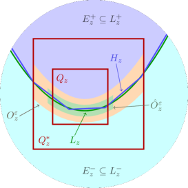
  Figure 4: Sketch of geometry in the construction of $U_{z}^{+}$ and $U_{z}^{-}$ in Step 3 in the proof of Theorem 1.1, assuming $n=2$, $R_{z}=\mathrm{Id}$, and that $L_{z}$ is the graph of a parabola. The set $E_{z}^{+}$ is the area above $L_{z}$ (inside the ball $B_{z}$), $O_{z}^{\varepsilon}$ is a neighborhood of $L_{z}$ intersected with the larger cube $Q_{z}^{*}$, and $\hat{O}_{z}^{\varepsilon}$ is a smaller neighborhood of $L_{z}$ intersected with a neighborhood of $Q_{z}$. The set $H_{z}$ is an approximation of $L_{z}$ with the graph of a piecewise affine function, and the part inside $Q_{z}$ belongs to $\hat{O}_{z}^{\varepsilon}$. Figure 3 shows how this construction interacts with the rest.

• Construction of $w_{z,\zeta}$ and $w_{\zeta}$. In this step we define an approximation ${w_{z,\zeta}}$ on each cube $Q_{z}$, for $z\in A_{\delta}$ and $\zeta\in B_{\varepsilon}$. This requires two different extensions of $u$ on different sets, a sketch is given in Figure 4.

  If $L_{z}\cap Q_{z}^{*}=\emptyset$ we set $w_{z,\zeta}=\Pi_{\varepsilon,\zeta}u$. The other case is more complex. We pick $y_{z}\in L_{z}\cap{Q_{z}^{*}}$, let $B_{z}:=B_{3\sqrt{n}\delta}(y_{z})$, so that $Q_{z}^{*}\subset\subset B_{z}\subset\Omega^{\prime}$, and consider the sets $E_{z}^{\pm}:=B_{z}\cap L_{z}^{\pm}$. One checks that, since $\varphi_{z}$ is $\theta$-Lipschitz with $\theta\leq\frac{1}{2}$, the sets $E_{z}^{\pm}$ are Lipschitz with a constant $C$. For this it is convenient to use that a bounded open set $A$ is Lipschitz if and only if there are a nontrivial open one-sided cone ${E}$ and $r>0$ such that $B_{r}(x)\cap(x+{E})\subset{A}$ and $B_{r}(x)\cap(x-{E})\cap{A}=\emptyset$ for all $x\in\partial{A}$, see [AFP00, Remark after Def. 2.60].

  Let $M>0$ be fixed, it will be chosen below depending only on the dimension $n$. By Theorem 3.5 there are $U^{\pm}_{z}\in SBV(\mathbb{R}^{n};\mathbb{R}^{m})$ which extend the restriction of $u$ to $E_{z}^{\pm}$, respectively. In particular, we have $U^{\pm}_{z}=u$ on $E_{z}^{\pm}$, and $|{DU^{+}_{z}}|(\partial E_{z}^{+})=|{DU^{-}_{z}}|(\partial E_{z}^{-})=0$. For $\varepsilon$ sufficiently small, letting ${O_{z}^{\varepsilon}:=(L_{z})_{2M\varepsilon}\cap Q_{z}^{*}}$, from $\bigcap_{\varepsilon>0}O_{z}^{\varepsilon}=L_{z}\cap Q_{z}^{*}\subset\partial E_{z}^{+}$ we obtain

  $$E_{|\cdot|^{p},g_{0}}[U^{+}_{z},{{O_{z}^{\varepsilon}}}]+|DU^{+}_{z}|({{O_{z}^{\varepsilon}}}){+\|\nabla u\|_{L^{p}(O_{z}^{\varepsilon})}^{p}+|Du|(O_{z}^{\varepsilon}\setminus L_{z})}\leq\frac{\delta^{n}\theta}{C_{\lambda}}$$ (4.59)

  for all $z$, and the same for $U^{-}_{z}$. If $\mathcal{H}^{n-1}(J_{u})<\infty$, then we also have for $\varepsilon>0$ small enough

  $${\sum_{z\in A_{\delta}}}\mathcal{H}^{n-1}(J_{U^{+}_{z}}\cap{O_{z}^{\varepsilon}})+\mathcal{H}^{n-1}(J_{U^{-}_{z}}\cap O_{z}^{\varepsilon})\leq{C\theta.}$$ (4.60)

  The function $w_{z,\zeta}$ will be defined as a discretization of $U_{z}^{+}$ on $H_{z}^{+}\cap Q_{z}$, and similarly with the other sign. By Proposition 4.3(iv) it depends on $U_{z}^{\pm}$ on a small neighborhood of the sets $H_{z}^{\pm}\cap Q_{z}$, and by Proposition 4.3(vi) the relevant properties of $w_{z,\zeta}$ can be estimated by corresponding properties of $U_{z}^{\pm}$ on $2{c_{*}}\varepsilon$-neighborhoods of $H_{z}^{\pm}\cap Q_{z}$ (see also (4.33)). Therefore we need to estimate $U^{\pm}_{z}$ on these sets.

  Let $\hat{O}_{z}^{\varepsilon}:=(L_{z})_{M\varepsilon}\cap(Q_{z})_{M\varepsilon}$. From (4.55), (4.56) and (4.57) we obtain $H_{z}\subseteq(L_{z})_{2\varepsilon}$ and $(H_{z}^{+})_{2{c_{*}}\varepsilon}\subseteq L_{z}^{+}\cup(L_{z})_{(2+2{c_{*}})\varepsilon}$, which imply

  $$(H_{z}^{+}\cap Q_{z})_{2{c_{*}}\varepsilon}\subseteq(L_{z}^{+}\cap Q_{z}^{*})\cup\hat{O}_{z}^{\varepsilon}$$ (4.61)

  and the same for the other sign, provided that $M\geq 2+2{c_{*}}$ and $\varepsilon$ is sufficiently small. Recalling (4.51), (4.59) in particular implies

  $$\begin{split}&\sum_{z\in A_{\delta}}\int_{J_{U_{z}^{+}}\cap{(H_{z}^{+}\cap Q_{z})_{2{c_{*}}\varepsilon}}}g_{0}(|[U_{z}^{+}]|)d\mathcal{H}^{n-1}\\ &+\sum_{z\in A_{\delta}}\int_{J_{U_{z}^{-}}\cap{(H_{z}^{-}\cap Q_{z})_{2{c_{*}}\varepsilon}}}g_{0}(|[U_{z}^{-}]|)d\mathcal{H}^{n-1}\leq C\theta\end{split}$$ (4.62)

  and

  $$\sum_{z\in A_{\delta}}\int_{{(H_{z}^{+}\cap Q_{z})_{2{c_{*}}\varepsilon}}}|\nabla U_{z}^{+}-\eta_{z}|^{p}dx+\int_{{(H_{z}^{-}\cap Q_{z})_{2{c_{*}}\varepsilon}}}|\nabla U_{z}^{-}-\eta_{z}|^{p}dx\leq C\theta.$$ (4.63)

  We next estimate the difference between $u$, $U^{+}_{z}$ and $U^{-}_{z}$ around $H_{z}$, this will be important after (4.104) (cf. (4.108)-(4.109)). We pick $x_{1},\dots,x_{K}\in L_{z}$ such that

  $$L_{z}\cap Q_{z}\subseteq\bigcup_{i}B_{i},\hskip 28.45274ptB_{i}:=B_{M\varepsilon}(x_{i}),$$ (4.64)

  and

  $$\hat{O}_{z}^{\varepsilon}\subseteq\bigcup_{i}B_{i}^{*},\hskip 28.45274ptB_{i}^{*}:=B_{2M\varepsilon}(x_{i}).$$ (4.65)

  This implies in particular $K\leq\frac{{C}{\delta^{n-1}}}{\varepsilon^{n-1}},$ for a constant ${C}$. We can pick the points so that the larger balls $B_{i}^{*}$ have finite overlap uniformly in $\varepsilon$, namely $\sum_{i=1}^{K}\chi_{B_{i}^{*}}\leq{C}$, and that they are all contained in $(Q_{z})_{3M\varepsilon}$. For $\varepsilon$ sufficiently small, $B_{i}^{*}\subseteq O_{z}^{\varepsilon}$. As $\varphi_{z}$ is ${\frac{1}{2}}$-Lipschitz, the sets $B_{i}^{*}\cap L_{z}^{+}$ and $B_{i}^{*}\cap L_{z}^{-}$ are uniformly Lipschitz, therefore there is a constant $C$ such that for any $i$ there are $h^{+}_{i}$, $h^{-}_{i}\in\mathbb{R}^{m}$ with

  $$\frac{1}{\varepsilon}\|u-h^{+}_{i}\|_{L^{1}(B_{i}^{*}\cap L_{z}^{+})}+\|Tu-h^{+}_{i}\|_{L^{1}(B_{i}^{*}\cap L_{z};\mathcal{H}^{n-1})}\leq C|Du|(B_{i}^{*}\cap L_{z}^{+}).$$ (4.66)

  In (4.66) we write $Tu$ for the inner trace on the boundary of $B_{i}^{*}\cap L_{z}^{+}$, which on $B_{i}^{*}\cap L_{z}$ coincides with $u^{+}$. The corresponding estimate holds with the other sign (then with $Tu=u^{-}$). This in particular implies

  $$\int_{B_{i}^{*}\cap L_{z}}|[u]-(h_{i}^{+}-h_{i}^{-})|d\mathcal{H}^{n-1}\leq C|Du|(B_{i}^{*}\setminus L_{z}).$$ (4.67)

  We observe that $\mathrm{Lip\,}(\varphi_{z})\leq{\frac{1}{2}}$ also implies for some constant $C$

  $$\frac{\varepsilon^{n}}{{C}}\leq|B_{i}^{*}\cap L_{z}^{+}|,\hskip 14.22636pt\frac{\varepsilon^{n}}{{C}}\leq|B_{i}^{*}\cap L_{z}^{-}|,$$ (4.68)

  as well as

  $$\frac{\varepsilon^{n-1}}{{C}}\leq\mathcal{H}^{n-1}(B_{i}\cap L_{z})\leq{C}\varepsilon^{n-1},\hskip 8.53581pt\frac{\varepsilon^{n-1}}{{C}}\leq\mathcal{H}^{n-1}(B_{i}\cap H_{z})\leq{C}\varepsilon^{n-1}.$$ (4.69)

  By Poincaré’s inequality applied to $U_{z}^{+}$ on $B_{i}^{*}$, using $u=U^{+}_{z}$ on $B_{i}^{*}\cap L_{z}^{+}$, (4.66) and (4.68),

  $$\|U^{{+}}_{z}-h_{i}^{{+}}\|_{L^{1}(B_{i}^{*})}\leq C\varepsilon|DU^{{+}}_{z}|(B_{i}^{*})$$ (4.70)

  and analogously for $U_{z}^{-}$ and $h_{i}^{-}$, so that

  $$\int_{B_{i}^{*}}|U_{z}^{+}-U_{z}^{-}-h_{i}^{+}+h_{i}^{-}|dx\leq C\varepsilon(|DU^{+}_{z}|+|DU^{-}_{z}|)(B_{i}^{*}).$$ (4.71)

  Finally, a direct application of Poincaré’s inequality to $U^{+}_{z}-u$ on $B_{i}^{*}$, using $u=U^{+}_{z}$ on $B_{i}^{*}\cap L_{z}^{+}$ and (4.68), leads to

  $$\int_{B_{i}^{*}}|U_{z}^{+}-u|dx\leq C\varepsilon(|DU^{+}_{z}|+|Du|)(B_{i}^{*}),$$ (4.72)

  obviously the same holds for $U^{-}_{z}$. Summing (4.72) over all balls shows that

  $$\|U_{z}^{+}-u\|_{L^{1}({\hat{O}_{z}^{\varepsilon}})}\leq C\varepsilon(|DU^{+}_{z}|+|Du|)(O_{z}^{\varepsilon})$$ (4.73)

  and the same for $U_{z}^{-}$. Summing instead (4.72) only over the balls with centers contained in ${(\partial Q_{z})_{3M\varepsilon}\cap L_{z}}$ gives

  $$\|U_{z}^{+}-u\|_{L^{1}((\partial Q_{z})_{M\varepsilon}\cap(L_{z})_{M\varepsilon})}\leq C\varepsilon{\left(|DU_{z}^{+}|+|Du|\right)((\partial Q_{z})_{5M\varepsilon}\cap O_{z}^{\varepsilon})},$$ (4.74)

  and the same bound for $U_{z}^{-}$.

  For $z\in A_{\delta}$ with $L_{z}\cap{Q_{z}^{*}}\neq\emptyset$ we define $w_{z,\zeta}:{\mathbb{R}^{n}}\to\mathbb{R}^{m}$ by

  $$w_{z,\zeta}:=\begin{cases}\Pi_{\varepsilon,\zeta}U^{+}_{z}&\text{ in }{H_{z}^{+}},\\ \Pi_{\varepsilon,\zeta}U^{-}_{z}&\text{ in }{H_{z}^{-},}\end{cases}$$ (4.75)

  we recall that if instead $L_{z}\cap{Q_{z}^{*}}=\emptyset$ we had set $w_{z,\zeta}=\Pi_{\varepsilon,\zeta}u$. In both cases, the function $w_{z,\zeta}$ is piecewise affine. For almost all $\zeta\in B_{\varepsilon}$ we have

  $${\mathcal{H}^{n-1}(J_{\Pi_{\varepsilon,\zeta}f}\cap H_{z})=\mathcal{H}^{n-1}(J_{\Pi_{\varepsilon,\zeta}f}\cap\partial Q_{z})=0}$$ (4.76)

  for any function $f$, and in particular for $U^{+}_{z}$ and $U^{-}_{z}$. With this choice, and recalling (4.58), $J_{w_{z,\zeta}}\cap\overline{Q}_{z}$ splits (up to $\mathcal{H}^{n-1}$-null sets) into the disjoint union of $J_{\Pi_{\varepsilon,\zeta}U^{+}_{z}}\cap H_{z}^{+}\cap Q_{z}$, $J_{\Pi_{\varepsilon,\zeta}U^{-}_{z}}\cap H_{z}^{-}\cap Q_{z}$, and a subset of $H_{z}\cap Q_{z}$, with

  $$[w_{z,\zeta}]=\Pi_{\varepsilon,\zeta}U^{+}_{z}-\Pi_{\varepsilon,\zeta}U^{-}_{z},\hskip 11.38109pt\text{$\mathcal{H}^{n-1}$-a.e. on $H_{z}\cap Q_{z}$.}$$ (4.77)

  By (4.56) and the fact that $\varphi_{z}$ is $\theta$-Lipschitz we also obtain

  $$|\nu_{w_{z,\zeta}}-R_{z}e_{n}|\leq C\theta\hskip 14.22636pt\text{$\mathcal{H}^{n-1}$-a.e. on }Q^{*}_{z}\cap H_{z}\cap J_{w_{z,\zeta}}.$$ (4.78)

  If $\mathcal{H}^{n-1}(J_{u})<\infty$ then using (4.29) separately on $U^{+}_{z}$ and $U^{-}_{z}$ (cf. the discussion to get (4.33)), then (4.61), $U^{+}=u$ on $L_{z}^{+}\cap Q_{z}$, and finally (4.52) and (4.60) we obtain

  $$\begin{split}&\fint_{B_{\varepsilon}}\sum_{z\in A_{\delta}}\mathcal{H}^{n-1}(\overline{Q}_{z}\cap H^{+}_{z}\cap J_{\Pi_{\varepsilon,\zeta}U^{+}_{z}})+\mathcal{H}^{n-1}(\overline{Q}_{z}\cap H^{-}_{z}\cap J_{\Pi_{\varepsilon,\zeta}U^{-}_{z}})d\zeta\\ &\leq C\sum_{z\in A_{\delta}}\mathcal{H}^{n-1}(Q_{z}^{*}\cap J_{u}\setminus L_{z})+\mathcal{H}^{n-1}(O_{z}^{\varepsilon}\cap J_{U^{+}_{z}})+\mathcal{H}^{n-1}(O_{z}^{\varepsilon}\cap J_{U^{-}_{z}})\leq C\theta.\end{split}$$ (4.79)

  We define $w^{0}_{\zeta}:=\Pi_{\varepsilon,\zeta}u$ and then $w_{\zeta}\in SBV(\bigcup_{z\in{A_{\delta}\cup A_{\delta}^{*}}}Q_{z};\mathbb{R}^{m})$ by setting $w_{\zeta}:={w_{z,\zeta}}$ on $Q_{z}$ if $z\in A_{\delta}$, and $w_{\zeta}:=w^{0}_{\zeta}$ if $z\in A_{\delta}^{*}$. For any $\zeta\in B_{\varepsilon}$, the function $w_{\zeta}$ is piecewise affine and obeys property (i). This concludes the construction of $w_{\zeta}$.

• Estimates on $w_{\zeta}$ and $\nabla w_{\zeta}$.

  We first check that we have not added too much jump on the boundary between adjacent cubes by replacing $w^{0}_{\zeta}$ by $w_{z,\zeta}$ and compute with (4.58) and (4.76)

  $$\begin{split}\int_{\partial Q_{z}}|w^{0}_{\zeta}-w_{z,\zeta}|d\mathcal{H}^{n-1}=&{\int_{\partial Q_{z}\cap H_{z}^{+}}|\Pi_{\varepsilon,\zeta}u-\Pi_{\varepsilon,\zeta}U^{+}_{z}|d\mathcal{H}^{n-1}}\\ &+{\int_{\partial Q_{z}\cap H_{z}^{-}}|\Pi_{\varepsilon,\zeta}u-\Pi_{\varepsilon,\zeta}U^{-}_{z}|d\mathcal{H}^{n-1}}\end{split}$$ (4.80)

  for $z\in A_{\delta}$. By estimate (4.31) with $\Sigma=\partial Q_{z}\cap H_{z}^{+}$,

  $$\begin{split}\fint_{B_{\varepsilon}}\int_{\partial Q_{z}\cap H_{z}^{+}}|w^{0}_{\zeta}-w_{z,\zeta}|d\mathcal{H}^{n-1}d\zeta\leq&\frac{C}{\varepsilon}\|u-U^{+}_{z}\|_{L^{1}((\partial Q_{z}\cap H_{z}^{+})_{{c_{*}}\varepsilon})}\\ &+C|D(u-U^{+}_{z})|((\partial Q_{z}\cap H_{z}^{+})_{2{c_{*}}\varepsilon}).\end{split}$$ (4.81)

  Recalling that $U_{z}^{+}=u$ on $E_{z}^{+}$ and (4.61), both domains can be restricted to $(\partial Q_{z})_{M\varepsilon}\cap(L_{z})_{M\varepsilon}$. The first term is estimated by (4.74), and we conclude

  $$\fint_{B_{\varepsilon}}\int_{\partial Q_{z}}|w^{0}_{\zeta}-w_{z,\zeta}|d\mathcal{H}^{n-1}d\zeta\leq C(|Du|+|DU^{+}_{z}|+|DU^{-}_{z}|)((\partial Q_{z})_{5M\varepsilon}\cap O_{z}^{\varepsilon})$$ (4.82)

  so that, using (4.54),

  $$\limsup_{\varepsilon\to 0}\sum_{z\in A_{\delta}}\fint_{B_{\varepsilon}}\int_{\partial Q_{z}}|w^{0}_{\zeta}-w_{z,\zeta}|d\mathcal{H}^{n-1}d\zeta{=0}.$$ (4.83)

  We next address the $L^{1}$ convergence. For any $z\in A_{\delta}$ for which $L_{z}\cap{Q_{z}^{*}}\neq\emptyset$, by the definition of $w_{\zeta}$ and Proposition 4.3(v), we have for $\mathcal{L}^{n}$-almost every $\zeta{\in B_{\varepsilon}}$

  $$\begin{split}\int_{Q_{z}}|w_{\zeta}-u|dx=&\int_{Q_{z}\cap H_{z}^{+}}|\Pi_{\varepsilon,\zeta}U_{z}^{+}-u|dx+\int_{Q_{z}\cap H_{z}^{-}}|\Pi_{\varepsilon,\zeta}U_{z}^{-}-u|dx\\ \leq&{\int_{Q_{z}\cap H_{z}^{+}}\left(|\Pi_{\varepsilon,\zeta}U_{z}^{+}-U_{z}^{+}|+|U_{z}^{+}-u|\right)}dx\\ &+{\int_{Q_{z}\cap H_{z}^{-}}\left(|\Pi_{\varepsilon,\zeta}U_{z}^{-}-U_{z}^{-}|+|U_{z}^{-}-u|\right)dx.}\end{split}$$ (4.84)

  We recall that $U^{+}_{z}=u$ on $Q_{z}\cap H_{z}^{+}\setminus\hat{O}_{z}^{\varepsilon}\subseteq E_{z}^{+}$ and (4.73) to obtain

  $$\begin{split}\int_{Q_{z}\cap H_{z}^{+}}|U_{z}^{+}-u|dx\leq&\|U_{z}^{+}-u\|_{L^{1}(\hat{O}_{z}^{\varepsilon})}\\ \leq&C\varepsilon(|DU^{+}_{z}|+|DU^{-}_{z}|+|Du|)(O_{z}^{\varepsilon}).\end{split}$$ (4.85)

  With (4.30) in Proposition 4.3,

  $${\begin{split}\fint_{B_{\varepsilon}}\int_{Q_{z}\cap H_{z}^{+}}|\Pi_{\varepsilon,\zeta}U_{z}^{+}-U_{z}^{+}|dx\,d\zeta&\leq C\varepsilon|DU_{z}^{+}|((Q_{z}\cap H_{z}^{+})_{2{c_{*}}\varepsilon})\\ &\leq C\varepsilon(|Du|(Q_{z}^{*})+|DU_{z}^{+}|(O_{z}^{\varepsilon}))\end{split}}$$ (4.86)

  and an analogous estimate holds for the term with the other sign. Recalling (4.59) we obtain

  $${\sum_{z\in A_{\delta}:\,L_{z}\cap Q_{z}\neq\emptyset}}\fint_{B_{\varepsilon}}\int_{{Q_{z}}}|w_{\zeta}-u|dx\,d\zeta\leq C\theta$$ (4.87)

  for $\varepsilon$ sufficiently small. If $L_{z}\cap Q_{z}^{*}=\emptyset$ or $z\in A_{\delta}^{*}$ the computation is simpler as $w_{\zeta}=w_{\zeta}^{0}=\Pi_{\varepsilon,\zeta}u$, and only (4.86) with $u$ in place of $U^{+}_{z}$ appears. From this we conclude that

  $$\fint_{B_{\varepsilon}}\int_{\Omega}|w_{\zeta}-u|dx\,d\zeta\leq C\theta.$$ (4.88)

  Moreover, from $w_{\zeta}=w_{\zeta}^{0}$ on $Q_{z}\setminus\hat{O}_{z}^{\varepsilon}$, from (4.59) and estimate (4.27) in Proposition 4.3(vi) we deduce

  $$\fint_{B_{\varepsilon}}\int_{\Omega}|\nabla w_{\zeta}-\nabla u|^{p}dx\,d\zeta$$

  $$\leq{C}\fint_{B_{\varepsilon}}\sum_{z\in A_{\delta}{\cup A_{\delta}^{*}}}{\Big{(}}\int_{Q_{z}}|{\nabla w_{\zeta}^{0}}-\nabla u|^{p}dx{+\int_{{\hat{O}_{z}^{\varepsilon}}}(|\nabla w_{\zeta}|^{p}+|\nabla u|^{p})dx\Big{)}}d\zeta$$

  $$\leq C\sum_{z\in A_{\delta}{\cup A_{\delta}^{*}}}\int_{(Q_{z})_{2{c_{*}}\varepsilon}}|\nabla u-\eta_{z}|^{p}dx{+C\theta}\leq C\theta,$$ (4.89)

  where the last estimate follows from (4.51), and the constant $C>0$ depends on $u$, on the dimension $n$, on $p$ and on $\Omega$.

• Definition of the deformation $\Phi$.

  We select $\delta^{\prime}\in(0,\delta)$ and define $\Phi:\mathbb{R}^{n}\to\mathbb{R}^{n}$ by

  $$\Phi(x):=x+\sum_{z\in A_{\delta}:{L_{z}\cap Q_{z}^{*}\neq\emptyset}}\alpha_{z}(x)R_{z}\left(\psi_{z}({(R_{z}^{T}{(x-x_{z})})^{\prime}})+{\beta}-\varphi_{z}({(R_{z}^{T}{(x-x_{z})})^{\prime}})\right)e_{n},$$ (4.90)

  where $(R_{z}^{T}x)^{\prime}$ denotes the first $n-1$ components of the vector $R_{z}^{T}x$ and we fixed a function $\alpha_{z}\in C^{\infty}_{c}(Q_{z};[0,1])$ with $\alpha_{z}=1$ on $Q_{z}^{\prime\prime}:=z+\gamma+(-\frac{\delta+\delta^{\prime}}{4},\frac{\delta+\delta^{\prime}}{4})^{n}$, $|{D}\alpha_{z}|\leq 6/(\delta-\delta^{\prime})$. The map $\Phi$ is Lipschitz since $\alpha_{z}$, $\psi_{z}$, $\varphi_{z}$ are, by definition $\Phi(x)=x$ for $x\not\in\Omega$, by (4.56) $|\Phi(x)-x|\leq{2\varepsilon}$ for all $x$, we can assume ${2\varepsilon}\leq(\delta-\delta^{\prime})/4$. For $\varepsilon$ sufficiently small, $\Phi(Q_{z})=Q_{z}$ for all $z\in\delta\mathbb{Z}^{n}$ by construction, and if we define $Q_{z}^{\prime}:=z+\gamma+(-\frac{\delta^{\prime}}{2},\frac{\delta^{\prime}}{2})^{n}\subset\subset Q_{z}^{\prime\prime}\subset\subset Q_{z}$, from (4.50), (4.56) and (4.57) we obtain

  $$H_{z}{\cap Q_{z}^{\prime}}=\Phi(L_{z}){\cap Q_{z}^{\prime}},{\text{ and }}{\Phi^{-1}(H_{z}){\cap Q_{z}^{\prime}}=L_{z}{\cap Q_{z}^{\prime}}.}$$ (4.91)

  In order to show that $\Phi$ is invertible with Lipschitz inverse it suffices to prove that ${D}\Phi$ is uniformly close to the identity. Indeed, using (4.56) we obtain

  $$\|{D}\Phi-\mathrm{Id}\|_{\infty}\leq \max_{z\in A_{\delta}}\|{D}\psi_{z}-{D}\varphi_{z}\|_{\infty}+\max_{z\in A_{\delta}}\|{D}\alpha_{z}\|_{\infty}(\|\psi_{z}-\varphi_{z}\|_{\infty}{+{|\beta|}})$$

  $$\leq \omega_{\varepsilon}+{\frac{{12\varepsilon}}{\delta-\delta^{\prime}}}\,.$$ (4.92)

  In particular, if $\varepsilon$ is sufficiently small on a scale depending on $\delta$ and $\delta^{\prime}$, we can ensure

  $$\|{D}\Phi-\mathrm{Id}\|_{\infty}\leq{\frac{1}{2}}\theta.$$ (4.93)

  Therefore,

  $$(1-{\frac{1}{2}}\theta)|x-y|\leq|\Phi(x)-\Phi(y)|\leq(1+\theta)|x-y|,$$

  which implies that $\Phi$ is globally bilipschitz. Property (iii) follows.

• Estimate of the jump energy.

  We are now able to estimate the energy of the jump contribution. We start to decompose it as

  $$\fint_{B_{\varepsilon}} \int_{\Omega\cap(J_{u}\cup\Phi^{-1}(J_{w_{\zeta}}))}g_{0}(|[u]-[w_{\zeta}]\circ\Phi|)\,d\mathcal{H}^{n-1}d\zeta$$

  $$\leq \fint_{B_{\varepsilon}}\sum_{z\in A_{\delta}\cup A_{\delta}^{*}}\int_{(J_{u}\cup\Phi^{-1}(J_{w_{\zeta}}))\cap Q_{z}}g_{0}(|[u]-{[w_{\zeta}]}\circ\Phi|)\,d\mathcal{H}^{n-1}d\zeta$$

  $$+\fint_{B_{\varepsilon}}\sum_{z\in A_{\delta}}\int_{\partial Q_{z}}g_{0}(|w_{z,\zeta}-w^{0}_{\zeta}|)d\mathcal{H}^{n-1}d\zeta$$ (4.94)

  where we separated the boundary contributions from the ones in the interior, then used $\Phi(x)=x$ on $\partial Q_{z}$, (4.54) to infer that $[u]=0$ almost everywhere on $\partial Q_{z}$, (4.76) to infer $[w_{z,\zeta}]=[w_{z}^{0}]=0$ almost everywhere on $\partial Q_{z}$, and finally used $|[w_{\zeta}]|\leq|w_{z,\zeta}-w_{\zeta}^{0}|+|w_{z^{\prime},\zeta}-w_{\zeta}^{0}|$ and subadditivity of $g_{0}$ on $\partial Q_{z}\cap\partial Q_{z^{\prime}}$ for $z,z^{\prime}\in A_{\delta}$, $|[w_{\zeta}]|=|w_{z,\zeta}-w_{\zeta}^{0}|$ on $\partial Q_{z}\cap\partial Q_{z^{\prime}}$ for $z\in A_{\delta}$, $z^{\prime}\in A_{\delta}^{*}$, and $|[w_{\zeta}]|=0$ on $\partial Q_{z}\cap\partial Q_{z^{\prime}}$ for $z,z^{\prime}\in A_{\delta}^{*}$.

  We start from the boundary term. From (4.45) we get

  $$\fint_{B_{\varepsilon}}\sum_{z\in A_{\delta}}\int_{\partial Q_{z}}g_{0}(|w_{z,\zeta}-w^{0}_{\zeta}|)d\mathcal{H}^{n-1}d\zeta\\ \leq\#A_{\delta}\mathcal{H}^{n-1}(\partial Q_{z})\lambda+C_{\lambda}{\fint_{B_{\varepsilon}}}\sum_{z\in A_{\delta}}\int_{\partial Q_{z}}|w_{z,\zeta}-w_{\zeta}^{0}|d\mathcal{H}^{n-1}{d\zeta}\leq{C\frac{\lambda}{\delta}}+{C}\theta,$$ (4.95)

  by (4.83) and choosing $\varepsilon$ sufficiently small. For $\lambda\leq\delta\theta$ the entire term is bounded by $C\theta$.

  We now turn to the first term of (6). We start from $z\in A_{\delta}$. Splitting

  $$J_{u}\cup\Phi^{-1}(J_{w_{\zeta}})= (J_{u}\cup\Phi^{-1}(J_{w_{\zeta}}))\cap(L_{z}\cup\Phi^{-1}(H_{z}))$$

  $$\cup(J_{u}\cup\Phi^{-1}(J_{w_{\zeta}}))\setminus(L_{z}\cup\Phi^{-1}(H_{z}))$$

  and using the subadditivity of $g_{0}$ to estimate the integral on the second set, we get

  $$\fint_{B_{\varepsilon}}\int_{(J_{u}\cup\Phi^{-1}(J_{w_{\zeta}}))\cap Q_{z}}g_{0}(|[u]-{[w_{\zeta}]}\circ\Phi|)\,d\mathcal{H}^{n-1}\,d\zeta\leq\mathrm{I}_{z}+\mathrm{II}_{z}+\mathrm{III}_{z}$$ (4.96)

  with

  $$\begin{split}\mathrm{I}_{z}:=&\fint_{B_{\varepsilon}}\int_{(L_{z}\cup\Phi^{-1}(H_{z}))\cap Q_{z}}g_{0}(|[u]-[w_{\zeta}]\circ\Phi|)\,d\mathcal{H}^{n-1}d\zeta,\\ \mathrm{II}_{z}:=&\int_{J_{u}\cap Q_{z}\setminus L_{z}}g_{0}(|[u]|)\,d\mathcal{H}^{n-1},\\ \mathrm{III}_{z}:=&\fint_{B_{\varepsilon}}\int_{\Phi^{-1}(J_{w_{\zeta}}\setminus H_{z})\cap Q_{z}}g_{0}(|[w_{\zeta}]\circ\Phi|)\,d\mathcal{H}^{n-1}\,d\zeta.\end{split}$$ (4.97)

  We start from $\mathrm{I}_{z}$. We add and subtract $s_{z}$, write

  $$\begin{split}\mathrm{I}_{z}\leq&\fint_{B_{\varepsilon}}\int_{(L_{z}\cup\Phi^{-1}(H_{z}))\cap Q_{z}}g_{0}(|[u]-s_{z}{|})+g_{0}(|[w_{\zeta}]\circ\Phi-s_{z}|)\,d\mathcal{H}^{n-1}d\zeta\end{split}$$ (4.98)

  and observe that

  $$g_{0}(|[u]-s_{z}|)\chi_{(\Phi^{-1}(H_{z})\setminus L_{z})\cap Q_{z}}\leq g_{0}(|[u]|)\chi_{(J_{u}\setminus L_{z})\cap Q_{z}}+g_{0}(|s_{z}|)\chi_{(\Phi^{-1}(H_{z})\setminus L_{z})\cap Q_{z}},$$

  and similarly for the other term. Therefore

  $$\begin{split}\mathrm{I}_{z}\leq&\mathrm{I}_{z}^{1}+\mathrm{I}_{z}^{2}+\mathrm{I}_{z}^{3}{+\mathrm{II}_{z}+\mathrm{III}_{z}},\end{split}$$ (4.99)

  where

  $$\mathrm{I}_{z}^{1}:=\int_{L_{z}\cap Q_{z}^{*}}g_{0}(|[u]-s_{z}|)\,d\mathcal{H}^{n-1},$$ (4.100)

  $$\mathrm{I}_{z}^{2}:=\fint_{B_{\varepsilon}}\int_{\Phi^{-1}(H_{z})\cap Q_{z}}g_{0}(|[w_{\zeta}]\circ\Phi-s_{z}|)\,d\mathcal{H}^{n-1}d\zeta,$$ (4.101)

  and

  $$\mathrm{I}_{z}^{3}:=g_{0}(|s_{z}|)\mathcal{H}^{n-1}((L_{z}\triangle\Phi^{-1}(H_{z}))\cap Q_{z}).$$ (4.102)

  First note that

  $$\sum_{z\in A_{\delta}}(\mathrm{I}^{1}_{z}+\mathrm{II}_{z})\leq C\theta$$ (4.103)

  thanks to (4.51). For $\mathrm{I}^{2}_{z}$ we use first the Coarea formula, (4.92) and (4.77) to obtain

  $$\begin{split}\mathrm{I}_{z}^{2}\leq&2\fint_{B_{\varepsilon}}\int_{H_{z}\cap Q_{z}}g_{0}(|\Pi_{\varepsilon,\zeta}(U_{z}^{+}-U_{z}^{-})-s_{z}|)\,d\mathcal{H}^{n-1}d\zeta.\end{split}$$ (4.104)

  We cover $H_{z}\cap Q_{z}$ with the balls $B_{i}$ introduced in (4.64), and start from estimating the term

  $$\mathrm{I}_{z}^{2}(B_{i}):=\fint_{B_{\varepsilon}}\int_{H_{z}\cap B_{i}}g_{0}(|\Pi_{\varepsilon,\zeta}(U_{z}^{+}-U_{z}^{-})-s_{z}|)\,d\mathcal{H}^{n-1}d\zeta.$$ (4.105)

  By subadditivity,

  $$g_{0}(|\Pi_{\varepsilon,\zeta}(U_{z}^{+}-U_{z}^{-})-s_{z}|)\leq g_{0}(|h_{i}^{+}-h_{i}^{-}-s_{z}|)+g_{0}(|\Pi_{\varepsilon,\zeta}(U_{z}^{+}-U_{z}^{-})-h_{i}^{+}+h_{i}^{-}|).$$ (4.106)

  The first term, using (4.69) twice and subadditivity, leads to

  $$\begin{split}&\int_{H_{z}\cap B_{i}}g_{0}(|h_{i}^{+}-h_{i}^{-}-s_{z}|)d\mathcal{H}^{n-1}\leq{C}\varepsilon^{n-1}g_{0}(|h_{i}^{+}-h_{i}^{-}-s_{z}|)\\ &\leq{C}\int_{L_{z}\cap B_{i}}[g_{0}(|[u]-s_{z}|)+g_{0}(|h_{i}^{+}-h_{i}^{-}-[u]|)]d\mathcal{H}^{n-1},\end{split}$$ (4.107)

  where the first integral is controlled by $\mathrm{I}_{z}^{1}$. Using (4.45) in the second term of (4.106) and the second term of (4.107), for any $\lambda>0$ we have

  $$\begin{split}\mathrm{I}_{z}^{2}(B_{i})\leq&{C}\int_{L_{z}\cap B_{i}}g_{0}(|[u]-s_{z}|)d\mathcal{H}^{n-1}+{C}\lambda\varepsilon^{n-1}\\ &+C_{\lambda}\int_{L_{z}\cap B_{i}}|h_{i}^{+}-h_{i}^{-}-[u]|\,d\mathcal{H}^{n-1}\\ &+C_{\lambda}\fint_{B_{\varepsilon}}\int_{H_{z}\cap B_{i}}|\Pi_{\varepsilon,\zeta}(U_{z}^{+}-U_{z}^{-}-h_{i}^{+}+h_{i}^{-})|\,d\mathcal{H}^{n-1}\,d\zeta.\end{split}$$ (4.108)

  The term in the second line can be estimated with (4.67). For the last line we use first (4.31) and then (4.71), and obtain

  $$\begin{split}&\fint_{B_{\varepsilon}}\int_{H_{z}\cap B_{i}}|\Pi_{\varepsilon,\zeta}(U_{z}^{+}-U_{z}^{-}-h_{i}^{+}+h_{i}^{-})|d\mathcal{H}^{n-1}\,d\zeta\\ &\leq\frac{C}{\varepsilon}\int_{B_{i}^{*}}|U_{z}^{+}-U_{z}^{-}-h_{i}^{+}+h_{i}^{-}|dx+C(|DU_{z}^{+}|+|DU_{z}^{-}|)(B_{i}^{*})\\ &\leq C(|DU_{z}^{+}|+|DU_{z}^{-}|)(B_{i}^{*}).\end{split}$$ (4.109)

  Using that $\mathrm{Lip\,}(\varphi_{z})\leq{\frac{1}{2}}$, (4.69) and $\sum_{i=1}^{K}\chi_{B_{i}^{*}}\leq{C}$, summing over $i$ yields

  $$\begin{split}\mathrm{I}_{z}^{2}\leq&{C}\mathrm{I}^{1}_{z}+C\lambda\delta^{n-1}+{C_{\lambda}}|Du|(O_{z}^{\varepsilon}\setminus L_{z})+{C_{\lambda}}(|DU_{z}^{+}|+|DU_{z}^{-}|)(O_{z}^{\varepsilon}),\end{split}$$ (4.110)

  so that by (4.59) summing on $z\in A_{\delta}$ we find for $\lambda\leq\delta\theta$ and $\varepsilon$ sufficiently small

  $$\sum_{z\in A_{\delta}}I_{z}^{2}\leq C\theta\,.$$

  We next turn to $\mathrm{I}_{z}^{3}$, and observe that by (4.91) and (4.92)

  $$\begin{split}\mathcal{H}^{n-1}((L_{z}\triangle\Phi^{-1}(H_{z}))\cap Q_{z})\leq&\mathcal{H}^{n-1}(L_{z}\cap Q_{z}\setminus Q_{z}^{\prime})+\mathcal{H}^{n-1}(\Phi^{-1}(H_{z})\cap Q_{z}\setminus Q_{z}^{\prime})\\ \leq&\mathcal{H}^{n-1}(L_{z}\cap Q_{z}\setminus Q_{z}^{\prime})+2\mathcal{H}^{n-1}(H_{z}\cap Q_{z}\setminus Q_{z}^{\prime}).\end{split}$$ (4.111)

  Therefore

  $$\mathrm{I}_{z}^{3}\leq{4}\max_{z\in A_{\delta}}g_{0}(|s_{z}|)\mathcal{H}^{n-1}\left((H_{z}\cup L_{z})\cap(Q_{z}\setminus Q_{z}^{\prime})\right).$$

  As $\mathcal{H}^{n-1}(\bigcup_{z\in A_{\delta}}(H_{z}\cup L_{z}){\cap Q_{z}})<\infty$ and $\bigcup_{\delta^{\prime}<\delta}Q_{z}^{\prime}=Q_{z}$, choosing $\delta^{\prime}$ sufficiently close to $\delta$ we have

  $${\sum_{z\in A_{\delta}}\mathcal{H}^{n-1}\left((H_{z}\cup L_{z})\cap(Q_{z}\setminus Q_{z}^{\prime})\right)\leq\theta\text{ and }}\sum_{z\in A_{\delta}}\mathrm{I}_{z}^{3}\leq\theta.$$ (4.112)

  Similarly, if $\mathcal{H}^{n-1}(J_{u})<\infty$, for $\delta^{\prime}$ sufficiently close to $\delta$ we have

  $$\mathcal{H}^{n-1}(J_{u}\cap\bigcup_{z\in A_{\delta}}(Q_{z}\setminus{Q_{z}^{\prime}}))\leq\theta.$$ (4.113)

  For $\mathrm{III}_{z}$ we use the Coarea formula and (4.92). We obtain

  $$\mathrm{III}_{z}\leq 2\fint_{B_{\varepsilon}}\int_{J_{w_{{z,\zeta}}}\cap Q_{z}{\setminus H_{z}}}g_{0}(|[w_{z,\zeta}]|)\,d\mathcal{H}^{n-1}\,d\zeta.$$ (4.114)

  Therefore $\mathrm{III}_{z}\leq 2\mathrm{III}_{z}^{+}+2\mathrm{III}_{z}^{-}$, with

  $$\mathrm{III}_{z}^{+}:=\fint_{B_{\varepsilon}}\int_{J_{\Pi_{\varepsilon,\zeta}U_{z}^{+}}\cap Q_{z}\cap H_{z}^{+}}{g_{0}(|[\Pi_{\varepsilon,\zeta}U_{z}^{+}]|)}\,d\mathcal{H}^{n-1}\,d\zeta,$$ (4.115)

  and similarly for $\mathrm{III}_{z}^{-}$. We use inequalities (4.28) to infer

  $$\sum_{z\in A_{\delta}}\mathrm{III}_{z}^{+}\leq C\sum_{z\in A_{\delta}}\int_{J_{U_{z}^{+}}\cap(H_{z}^{{+}}\cap Q_{z})_{2{c_{*}}\varepsilon}}g_{0}(|[U_{z}^{+}]|)\,d\mathcal{H}^{n-1},$$ (4.116)

  and the same for $\mathrm{III}_{z}^{-}$. Both can be estimated via (4.62), we conclude that

  $$\sum_{z\in A_{\delta}}\mathrm{III}_{z}\leq C\theta.$$ (4.117)

  We next treat the bulk term in (6) in the case $z\in A_{\delta}^{*}$. Since $\Phi(x)=x$ and ${w_{\zeta}}={w_{\zeta}^{0}}$ on $Q_{z}$, recalling Proposition 4.3 (iii),

  $$\fint_{B_{\varepsilon}}\int_{(J_{u}\cup J_{w_{\zeta}^{0}})\cap Q_{z}}g_{0}(|[u]-{[w_{\zeta}^{0}]}{|})\,d\mathcal{H}^{n-1}\,d\zeta\leq\mathrm{IV}_{z}+\mathrm{V}_{z},$$ (4.118)

  where

  $$\begin{split}\mathrm{IV}_{z}:=&\int_{J_{u}\cap Q_{z}}g_{0}(|[u]|)\,d\mathcal{H}^{n-1},\\ \mathrm{V}_{z}:=&\fint_{B_{\varepsilon}}\int_{J_{w_{\zeta}^{0}}\cap Q_{z}}g_{0}(|[w_{\zeta}^{0}]|)\,d\mathcal{H}^{n-1}\,d\zeta.\end{split}$$ (4.119)

  As for $\mathrm{III}_{z}^{{+}}$, we use inequality (4.28) in Proposition 4.3 and obtain

  $$\mathrm{V}_{z}\leq C\int_{J_{u}\cap(Q_{z})_{2{c_{*}}\varepsilon}}g_{0}(|[u]|)\,d\mathcal{H}^{n-1}$$ (4.120)

  so that

  $$\sum_{z\in A_{\delta}^{*}}(\mathrm{IV}_{z}+\mathrm{V}_{z})\leq C\mu_{u}(\bigcup_{z\in A_{\delta}^{*}}(Q_{z})_{2{c_{*}}\varepsilon})\leq C\mu_{u}((\partial\Omega)_{3\sqrt{n}\delta})\leq C\theta,$$ (4.121)

  for $\varepsilon$ sufficiently small, where in the last step we used (4.48). Combining the previous estimates, (6) yields

  $$\fint_{B_{\varepsilon}}\int_{{\Omega\cap}(J_{u}\cup\Phi^{-1}(J_{w_{\zeta}}))}g_{0}(|[u]-[w_{\zeta}]\circ\Phi|)\,d\mathcal{H}^{n-1}d\zeta\leq C\theta\,.$$ (4.122)

  We claim next that for $\varepsilon$ sufficiently small

  $$\fint_{B_{\varepsilon}}\int_{\Omega\cap(J_{u}\cup\Phi^{-1}(J_{w_{\zeta}}))}g_{0}(|[u]|+|[w_{\zeta}]\circ\Phi|)\,\bigl{|}\nu_{u}-\nu_{w_{\zeta}}\circ\Phi\bigr{|}\,d\mathcal{H}^{n-1}d\zeta\leq C\theta\,.$$ (4.123)

  Thanks to subadditivity and monotonicity of $g_{0}$, (4.122) implies that it suffices to prove

  $$\fint_{B_{\varepsilon}}\int_{\Omega\cap(J_{u}\cap\Phi^{-1}(J_{w_{\zeta}}))}g_{0}(|[u]|)\,\bigl{|}\nu_{u}-\nu_{w_{\zeta}}\circ\Phi\bigr{|}\,d\mathcal{H}^{n-1}d\zeta\leq C\theta\,.$$ (4.124)

  Similarly, by (4.103), (4.112) and (4.121) it suffices prove

  $$\sum_{z\in A_{\delta}}\fint_{B_{\varepsilon}}\int_{Q_{z}\cap L_{z}\cap\Phi^{-1}(H_{z})}g_{0}(|[u]|)|\nu_{u}-\nu_{w_{\zeta}}\circ\Phi|d\mathcal{H}^{n-1}\,d\zeta\leq C\theta\,.$$ (4.125)

  From (4.78) we obtain that $|\nu_{w_{\zeta}}\circ\Phi-R_{z}e_{n}|\leq\theta$ almost everywhere on $Q_{z}\cap\Phi^{-1}(H_{z})$. The claim follows then from (4.51) and integrability of $g_{0}(|[u]|)$.

• Choice of $\zeta$, conclusion of the proof.

  From (4.88), (4) , (4.122) and (4.123), it is easy to check that there is a subset $\tilde{B}\subset B_{\varepsilon}$, with $|\tilde{B}|/|B_{\varepsilon}|>1/2$, such that for all $\zeta\in\tilde{B}$ (4.76) holds and we have

  $$\int_{\Omega}|w_{\zeta}-u|dx\leq C\theta,$$

  $$\int_{\Omega}|\nabla w_{\zeta}-\nabla u|^{p}dx\leq C\theta,$$

  $$\int_{{\Omega\cap}(J_{u}\cup\Phi^{-1}(J_{w_{\zeta}}))}g_{0}(|[u]-[w_{\zeta}]\circ\Phi|)\,d\mathcal{H}^{n-1}\leq C\theta,$$

  $$\int_{{\Omega\cap}(J_{u}\cup\Phi^{-1}(J_{w_{\zeta}}))}g_{0}(|[u]|+|[w_{\zeta}]\circ\Phi|)\,|\nu_{u}-\nu_{w_{\zeta}}\circ\Phi|\,d\mathcal{H}^{n-1}\leq C\theta.$$

  If $\mathcal{H}^{n-1}(J_{u})<\infty$ then, using (4.79), we can choose $\tilde{B}$ so that additionally

  $$\sum_{z\in A_{\delta}}\mathcal{H}^{n-1}(\overline{Q}_{z}\cap J_{w_{\zeta}}\setminus H_{z})\leq C\theta,$$

  which by the Coarea formula as usual implies

  $$\sum_{z\in A_{\delta}}\mathcal{H}^{n-1}(\overline{Q}_{z}\cap\Phi^{-1}(J_{w_{\zeta}}\setminus H_{z}))\leq C\theta.$$ (4.126)

  Properties (ii), (iii) and (v) follow; (i) and (iv) had already been proven. Property (vii) is immediate.

  It remains to prove (vi). We assume that $\mathcal{H}^{n-1}(J_{u})<\infty$ and start from a bound on $\Phi^{-1}(J_{w_{\zeta}})\setminus J_{u}$. We split the jump set of $w_{\zeta}$ into the contribution inside each cube $Q_{z}$, for $z\in A_{\delta}^{*}\cup A_{\delta}$, and then for each $z\in A_{\delta}$, we split the jump set $J_{w_{\zeta}}$ into the part in $H_{z}$ and the rest. We obtain

  $$\begin{split}&\mathcal{H}^{n-1}(\Omega\cap\Phi^{-1}(J_{w_{\zeta}})\setminus J_{u})\leq\sum_{z\in A^{*}_{\delta}}\mathcal{H}^{n-1}(\overline{Q}_{z}\cap\Phi^{-1}(J_{w_{\zeta}}))\\ &\hskip 5.69054pt+\sum_{z\in A_{\delta}}\Big{(}\mathcal{H}^{n-1}(\overline{Q}_{z}\cap\Phi^{-1}(H_{z})\setminus J_{u})+\mathcal{H}^{n-1}(\overline{Q}_{z}\cap\Phi^{-1}(J_{w_{\zeta}}\setminus H_{z}))\Big{)}.\end{split}$$ (4.127)

  In the first term in the second line, we use (4.58) to drop the part on $\partial{Q_{z}}$ and then separate the contributions inside and outside $L_{z}$. Equation (4.91) ensures that $Q_{z}^{\prime}\cap\Phi^{-1}(H_{z})\setminus L_{z}=\emptyset$. We obtain

  $$\begin{split}&\sum_{z\in A_{\delta}}\mathcal{H}^{n-1}(\overline{Q}_{z}\cap\Phi^{-1}(H_{z})\setminus J_{u})\\ &\leq\sum_{z\in A_{\delta}}\Big{(}\mathcal{H}^{n-1}(Q_{z}\cap L_{z}\setminus J_{u})+\mathcal{H}^{n-1}(Q_{z}\cap\Phi^{-1}(H_{z})\setminus Q_{z}^{\prime})\Big{)}\leq C\theta,\end{split}$$ (4.128)

  where the last inequality follows from (4.52), (4.112) and the Coarea formula. The other two terms in (LABEL:Jw-Ju1) can be bounded by (4.126) and (4.49), and we conclude

  $$\mathcal{H}^{n-1}(\Omega\cap\Phi^{-1}(J_{w_{\zeta}})\setminus J_{u})\leq C\theta.$$ (4.129)

  The converse inequality is proven by a different argument based on lower semicontinuity. As discussed in the first lines of the proof, taking a sequence $\theta_{j}\to 0$ we obtain a sequence $w_{j}$ which has all stated properties, except that (vi) is replaced by the weaker assertion

  $$\limsup_{j}\mathcal{H}^{n-1}(\Omega\cap\Phi_{j}^{-1}(J_{w_{j}})\setminus J_{u})=0.$$ (4.130)

  In particular $w_{j}$ converges to $u$ in $L^{1}(\Omega;\mathbb{R}^{m})$, and since $\nabla w_{j}$ converges to $\nabla u$ strongly in $L^{p}(\Omega;\mathbb{R}^{m\times n})$, with $p\in[1,\infty)$ given, there is a function $f:\mathbb{R}^{m\times n}\to[0,\infty)$ with superlinear growth at infinity such that

  $$\limsup_{j}\int_{\Omega}f(\nabla w_{j})dx+\mathcal{H}^{n-1}(\Omega\cap J_{w_{j}})<\infty$$ (4.131)

  (if $p>1$, then $f(\xi):=|\xi|^{p}$ itself will do; if $p=1$, de la Vallée-Poussin Theorem gives the conclusion). By the $SBV$ closure and lower semicontinuity theorem [AFP00, Theorem 4.7], we deduce

  $$\mathcal{H}^{n-1}(\Omega\cap J_{u})\leq\liminf_{j}\mathcal{H}^{n-1}(\Omega\cap J_{w_{j}})=\liminf_{j}\mathcal{H}^{n-1}(\Omega\cap\Phi_{j}^{-1}(J_{w_{j}})),$$ (4.132)

  where the last equality can be obtained from the area formula and (iv). By additivity of $\mathcal{H}^{n-1}$,

  $$\begin{split}\mathcal{H}^{n-1}(\Omega\cap J_{u}\setminus\Phi_{j}^{-1}(J_{w_{j}}))=&\mathcal{H}^{n-1}(\Omega\cap J_{u})-\mathcal{H}^{n-1}(\Omega\cap\Phi_{j}^{-1}(J_{w_{j}}))\\ &+\mathcal{H}^{n-1}(\Omega\cap\Phi_{j}^{-1}(J_{w_{j}})\setminus J_{u}).\end{split}$$ (4.133)

  Using first (4.132) and then (4.130),

  $$\limsup_{j}\mathcal{H}^{n-1}(\Omega\cap J_{u}\setminus\Phi_{j}^{-1}(J_{w_{j}}))\leq\limsup_{j}\mathcal{H}^{n-1}(\Omega\cap\Phi_{j}^{-1}(J_{w_{j}})\setminus J_{u})=0,$$ (4.134)

  which concludes the proof.

∎

References

- [AABU22] L. Ambrosio, S. Aziznejad, C. Brena, and M. Unser. Linear inverse problems with Hessian-Schatten total variation. Preprint arXiv:2210.04077, 2022.
- [ABC23] L. Ambrosio, C. Brena, and S. Conti. Functions with bounded Hessian-Schatten variation: density, variational and extremality properties. Preprint arXiv:2302.12554, 2023.
- [ADC05] M. Amar and V. De Cicco. A new approximation result for BV-functions. Comptes Rendus Mathematique, 340:735–738, 2005.
- [AF02] R. Alicandro and M. Focardi. Variational approximation of free-discontinuity energies with linear growth. Commun. Contemp. Math., 4:685–723, 2002.
- [AFP00] L. Ambrosio, N. Fusco, and D. Pallara. Functions of bounded variation and free discontinuity problems. Oxford Mathematical Monographs. The Clarendon Press, Oxford University Press, New York, 2000.
- [Amb89] L. Ambrosio. A compactness theorem for a new class of functions of bounded variation. Boll. Un. Mat. Ital. B (7), 3:857–881, 1989.
- [BBB95] G. Bouchitté, A. Braides, and G. Buttazzo. Relaxation results for some free discontinuity problems. J. Reine Angew. Math., 458:1–18, 1995.
- [BC94] A. Braides and A. Coscia. The interaction between bulk energy and surface energy in multiple integrals. Proc. Roy. Soc. Edinburgh Sect. A, 124:737–756, 1994.
- [BCG14] G. Bellettini, A. Chambolle, and M. Goldman. The -limit for singularly perturbed functionals of Perona-Malik type in arbitrary dimension. Math. Models Methods Appl. Sci., 24:1091–1113, 2014.
- [BCP96] A. Braides and V. Chiadò Piat. Integral representation results for functionals defined on . J. Math. Pures Appl. (9), 75:595–626, 1996.
- [Bra98] A. Braides. Approximation of free-discontinuity problems, volume 1694 of Lecture Notes in Mathematics. Springer-Verlag, Berlin, 1998.
- [CC19] A. Chambolle and V. Crismale. A density result in with applications to the approximation of brittle fracture energies. Archive for Rational Mechanics and Analysis, 232:1329–1378, 2019.
- [CFI17] S. Conti, M. Focardi, and F. Iurlano. Integral representation for functionals defined on in dimension two. Arch. Ration. Mech. Anal., 223:1337–1374, 2017. Preprint arXiv:1510.00145.
- [CFI19] S. Conti, M. Focardi, and F. Iurlano. Approximation of fracture energies with -growth via piecewise affine finite elements. ESAIM: COCV, 25:34, 2019.
- [CFI22] S. Conti, M. Focardi, and F. Iurlano. Phase-field approximation of a vectorial, geometrically nonlinear cohesive fracture energy. Preprint arXiv:2205.06541, 2022.
- [CFI23] S. Conti, M. Focardi, and F. Iurlano. Superlinear cohesive fracture models as limits of phase field functionals. In preparation, 2023.
- [Cha04] A. Chambolle. An approximation result for special functions with bounded deformation. J. Math. Pures Appl. (9), 83:929–954, 2004.
- [CM08] S. Conti and F. Maggi. Confining thin elastic sheets and folding paper. Arch. Rat. Mech. Anal., 187:1–48, 2008.
- [Cor97] G. Cortesani. Strong approximation of functions by piecewise smooth functions. Annali dell’Università di Ferrara, 43:27–49, 1997.
- [Cri19] V. Crismale. On the approximation of SBD functions and some applications. SIAM Journal on Mathematical Analysis, 51:5011–5048, 2019.
- [CS11] F. Cagnetti and L. Scardia. An extension theorem in SBV and an application to the homogenization of the Mumford–Shah functional in perforated domains. Journal de mathématiques pures et appliquées, 95:349–381, 2011.
- [CT99] G. Cortesani and R. Toader. A density result in SBV with respect to non-isotropic energies. Nonlinear Anal., 38:585–604, 1999.
- [DGA88] E. De Giorgi and L. Ambrosio. New functionals in the calculus of variations. Atti Accad. Naz. Lincei Rend. Cl. Sci. Fis. Mat. Nat. (8), 82:199–210 (1989), 1988.
- [DPFP17] G. De Philippis, N. Fusco, and A. Pratelli. On the approximation of SBV functions. Atti Accad. Naz. Lincei Rend. Lincei Mat. Appl., 28:369–413, 2017.
- [Fed69] H. Federer. Geometric measure theory. Die Grundlehren der mathematischen Wissenschaften, Band 153. Springer-Verlag New York, Inc., New York, 1969.
- [Fri18] M. Friedrich. A piecewise Korn inequality in SBD and applications to embedding and density results. SIAM Journal on Mathematical Analysis, 50:3842–3918, 2018.
- [FS18] M. Friedrich and F. Solombrino. Quasistatic crack growth in 2d-linearized elasticity. Annales de l’Institut Henri Poincaré C, Analyse non linéaire, 35:27–64, 2018.
- [Iur14] F. Iurlano. A density result for GSBD and its application to the approximation of brittle fracture energies. Calc. Var. Partial Differential Equations, 51:315–342, 2014.
- [KR16] J. Kristensen and F. Rindler. Piecewise affine approximations for functions of bounded variation. Numer. Math., 132:329–346, 2016.