From Complexity to Clarity: Analytical Expressions of Deep Neural Network Weights via Clifford’s Geometric Algebra and Convexity

Abstract

In this paper, we introduce a novel analysis of neural networks based on geometric (Clifford) algebra and convex optimization. We show that optimal weights of deep ReLU neural networks are given by the wedge product of training samples when trained with standard regularized loss. Furthermore, the training problem reduces to convex optimization over wedge product features, which encode the geometric structure of the training dataset. This structure is given in terms of signed volumes of triangles and parallelotopes generated by data vectors. The convex problem finds a small subset of samples via $\ell_{1}$ regularization to discover only relevant wedge product features. Our analysis provides a novel perspective on the inner workings of deep neural networks and sheds light on the role of the hidden layers.

1 Introduction

While there has been a lot of progress in developing deep neural networks (DNNs) to solve practical machine learning problems [1, 2, 3], the inner workings of neural networks is not well understood. A foundational theory for understanding how neural networks work is still lacking despite extensive research over several decades. In this paper, we provide a novel analysis of neural networks based on geometric algebra and convex optimization. We show that weights of deep ReLU neural networks learn the wedge product of a subset of training samples when trained by minimizing standard regularized loss functions. Furthermore, the training problem reduces to convex optimization over wedge product features, which encode the geometric structure of the training dataset. This structure is given in terms of signed volumes of triangles and parallelotopes generated by data vectors. Our analysis provides a novel perspective on the inner workings of deep neural networks and sheds light on the role of the hidden layers.

1.1 Prior work

The quest to understand the internal workings of neural networks (NNs) has led to numerous theoretical and empirical studies over the years. A striking discovery is the phenomenon of ”neural collapse,” observed when the representations of individual classes in the penultimate layer of a deep neural network tend to a point of near-indistinguishability [4]. Despite this insightful finding, the underlying mechanism that enables this collapse is yet to be fully understood. Linearizations and infinite-width approximations have been proposed to explain the inner workings of neural networks [5, 6, 7]. However, these approaches often simplify the rich non-linear interactions inherent in deep networks, potentially missing out on the full spectrum of dynamics and behaviors exhibited during training and inference.

The relationship between neural networks and geometric structures has been another area of research focus. Convex optimization and convex geometry viewpoint of neural networks has been extensively studied in recent work [8, 9, 10, 11, 12, 13, 14, 15, 16]. However, previous works have focused mostly on computational aspects of convex reformulations and left understanding the inner workings as an open problem.

1.2 Summary of results

The work in this paper diverges from other approaches by using Clifford’s geometric algebra and convex analysis to characterize the structure of optimal neural network weights. We show that the optimal weights for deep ReLU neural networks can be found via the closed-form formula, $x_{j_{1}}\wedge\ldots\wedge x_{j_{k}}$, known as a k-blade in geometric algebra, with $\wedge$ signifying the wedge product. For each individual neuron, this expression involves a special subset of training samples indexed by $(j_{1},\ldots,j_{k})$, which may vary across neurons. Surprisingly, the entire network training procedure can be reinterpreted as a purely discrete problem that identifies this unique subset for every neuron. Moreover, we show that this problem can be cast as a Lasso variable selection procedure over wedge product features, algebraically encoding the geometric structure of the training dataset. Contrary to the common belief that neurons maximize response by aligning with corresponding input samples, according to our theory, each neuron remains orthogonal to the data points within this special subset due to the properties of the wedge product.

Our results show that within a deep neural network, when an input sample $x$ is multiplied with a trained neuron, it yields the product $x^{T}\star(x_{j_{1}}\wedge\ldots\wedge x_{j_{k}})$. Leveraging geometric algebra, this product can be shown to be equal to the signed distance between $x$ and the linear span of the point set ${x_{j_{1}},\ldots,x_{j_{k}}}$, scaled by the length of the neuron. This allows the neurons to measure the oriented distance between the input sample and the affine hull of the special subset of samples. Rectified Linear Unit (ReLU) activations transform negative distances, representing inverse orientations, to zero. When this operation is extended across a collection of neurons within a layer, the layer’s output effectively translates the input sample into a coordinate system defined by the affine hulls of a special subset of training samples. Consequently, each layer is fundamentally tied solely to a specific subset of the training data. This subset can be identified by examining the weights of a trained network. Furthermore, with access to these training samples, the entirety of the network weights can be reconstructed using the wedge product formula. This geometric elucidation sheds fresh light on the mysterious roles played by the hidden layers in DNNs.

1.3 Notation

In our notation, lower-case letters are employed to represent vectors, while upper-case letters denote matrices. We use lower-case letters for vectors and upper-case letters for matrices. The notation $[n]$ represents integers from $1$ to $n$. We use a multi-index notation to simplify indexing matrices and tensors. Specifically, $j=(j_{1},...,j_{k})$ is a multi-index and $\sum_{j}$ denotes the summation operator over all indices included in the multi-index $j$, i.e., $\sum_{j_{1}}\cdots\sum_{j_{k}}$. Given a matrix $K\in\mathbb{R}^{n\times p}$, an ordinary index $i\in[n]$, and a multi-index $j=(j_{1},...,j_{k})$ where $j_{i}\in[d_{i}]~{}\forall i\in[k]$, the notation $K_{ij}$ denotes the $(i,v(j_{1},...,j_{k}))$-th entry of this matrix, where $v$ represents the function that maps indices $(j_{1},...,j_{k})$ to a one-dimensional index according to a column-major ordering. Formally, we can define $v(j_{1},...,f_{d}):=(j_{1}-1)+(j_{2}-1)d_{1}+(j_{3}-1)d_{1}d_{2}+...+(j_{n}-1)d_{1}d_{2}...d_{k-1}$. We allow the use of multi-index and ordinary indices together, e.g., $\sum_{j}a_{j}v_{j_{1}}\cdots v_{j_{d}}=\sum_{j_{1},\cdots j_{d}}a_{(j_{1},\cdots,j_{d})}v_{j_{1}}\cdots v_{j_{d}}$. The notation $K_{i\cdot}$ denotes the $i$-th row of $K$. The notation $K_{\cdot j}$ denotes the $j$-th column of $K$. The $p$-norm of a $d$-dimensional vector $w$ for some $p\in(0,\infty)$ is represented by $\|w\|_{p}$, and it is defined as $\|w\|_{p}\triangleq(\sum_{i=1}^{d}|w_{i}|^{p})^{1/p}$. In addition, we use the notation $\|w\|_{0}$ to denote the number of non-zero entries of $w$ and $\|w\|_{\infty}$ to denote the maximum absolute value of the entries of $w$. We use the notation $\mathcal{B}_{p}^{d}$ for the unit $p$-norm ball in $\mathbb{R}^{d}$ given by $\{w\in\mathbb{R}^{d}:\|w\|_{p}\leq 1\}$. The notation $\mathbf{dist}(\mathbf{x},\mathcal{Y})$ is used for the minimum Euclidean distance between a vector $\mathbf{x}\in\mathbb{R}^{d}$ and a subset $\mathcal{Y}\subseteq\mathbb{R}^{d}$. $\mathbf{Vol}(\mathcal{C})$ denotes $d$-volume of a subset $\mathcal{C}\subseteq\mathbb{R}^{d}$. The notation $(\cdot)_{+}$ is used the positive part of a real number. When applied to a scalar multiple of a pseudoscalar in a geometric algebra $\mathbb{G}^{d}$ such as $\alpha\mathbf{I}\in\mathbb{G}^{d}$, where $\mathbf{I}^{2}=\pm 1$, the notation $(\alpha\mathbf{I})_{+}=(\alpha)_{+}\in\mathbb{R}$ represents the positive part of the scalar component of $\mathbf{I}$. We use the notation $\mathbf{Vol}_{+}(\cdot)=(\mathbf{Vol}(\cdot))_{+}$ to denote the positive part of signed volumes. We extend this notation to other functions, e.g., ${\det}_{+}(\cdot)$ denotes the positive part of the determinant, and $\mathbf{dist}_{+}(\cdot,\cdot)$ denotes the positive part of the Euclidean distance. $\mathbf{diam}(S)$ denotes the Euclidean diameter of a subset $S\subseteq\mathbb{R}^{d}$. $\mathbf{Span}(S)$ and $\mathbf{Aff}(S)$ denote the linear span and affine hull of a set of vectors $S$ respectively.

2 Setting and Methodology

2.1 Preliminaries

Consider a deep neural network

$$f(x)=\sigma(W^{(L)}\cdots\sigma(W^{(1)}x+b_{1})\cdots+b^{(L)}),$$ (1)

where $\sigma:\mathbb{R}\to\mathbb{R}$ is a non-linear activation function, $W^{(1)},\ldots,W^{(L)}$ are trainable weight matrices, $b_{1},...,b_{L}$ are trainable bias vectors and $x\in\mathbb{R}^{d}$ is the input. The activation function $\sigma(\cdot)$ operates on each element individually.

Training two-layer ReLU networks

We will begin by examining the regularized training objective for a two-layer neural network with ReLU activation function and $m$ hidden neurons.

$$p^{*} \triangleq\min_{{W}^{(1)},\,{W}^{(2)},\,b}\ell\Big{(}\sum_{j=1}^{m}\sigma({X}{W}^{(1)}_{j}+{1}b_{j}){W}^{(2)}_{j},y\Big{)}+\lambda\sum_{j=1}^{m}\|{W}^{(1)}_{j}\|_{p}^{2}+\|{W}^{(2)}_{j}\|_{p}^{2},$$ (2)

where ${X}\in\mathbb{R}^{n\times d}$ is the training data matrix, ${W}^{(1)}\in\mathbb{R}^{d\times m}$ and ${W}^{(2)}\in\mathbb{R}^{m\times c}$ are trainable weights, $\ell(\cdot,y)$ is a convex loss function, $y\in\mathbb{R}^{n}$ is a vector containing the training labels, and $\lambda>0$ is the regularization parameter. Here we use the $p$-norm in the regularization of the weights. Initially, we will assume an output dimension of $c=1$, and we will extend this to arbitrary values of $c$. Typical loss functions used in practice include squared loss, logistic loss, cross-entropy loss and hinge loss, which are convex functions.

When $p=2$, the objective (2) reduces to the standard weight decay regularized NN problem

$$p^{*} =\min_{\theta,\,b}\ell\big{(}f_{\theta,b}(X),y\big{)}+\lambda\|\theta\|_{2}^{2}.$$ (3)

Here, $\theta$ is a vector containing the weights ${W}_{1}$ and $W_{2}$ in vectorized form and

$$f_{\theta,\,b}(X)\triangleq\sum_{j=1}^{m}\sigma({X}{W}^{(1)}_{j}+{1}b_{j}){W}^{(2)}_{j}.$$ (4)

When $b$ is set to zero, we refer to the neurons in the first layer as the bias-free neurons. When $b$ is not set to zero, we refer to the neurons in the first layer as the biased neurons. Note that the bias terms are excluded from the regularization.

Training deep ReLU neural networks

We will extend our analysis by also considering the objective in (3) using the deeper network model show in (1). It will be shown by a simple induction that the structural results for two-layer networks applies to blocks of layers in arbitrarily deep ReLU networks.

Augmented data matrix

For reasons that will become clear later, we augment the set of $n$ training data vectors of dimension $d$ by including $d$ additional vectors from the standard basis of $\mathbb{R}^{d}$ and let $\tilde{n}=n+d$. Specifically, we define the augmented data samples as $\{x_{i}\}_{i=1}^{n+d}=\{x_{i}\}_{i=1}^{n}\cup\{e_{i}\}_{i=1}^{d}$, where $x_{i}\in\mathbb{R}^{d}$ represents the original training data points for $1\leq i\leq n$ and $e_{i}$ is the $i$-th standard basis vector in $\mathbb{R}^{d}$ for $i\geq n$. We define $\tilde{X}=[x_{1},\cdots,x_{n+d}]^{T}$, as this notation simplifies subsequent expressions.

2.2 Geometric Algebra

Clifford’s Geometric Algebra (GA) is a mathematical framework that extends the classical vector and linear algebra and provides a unified language for expressing geometric constructions and ideas [17]. GA has found applications in classical and relativistic physics, quantum mechanics, computer graphics, robotics and numerous other fields [18, 19]. GA enables encoding geometric transformations in a form that is highly intuitive and convenient. More importantly, GA unifies several mathematical concepts, including complex numbers, quaternions, and tensors and provides a powerful toolset.

We consider GA over a $d$-dimensional Euclidean space, denoted as $\mathbb{G}^{d}$. The fundamental object in $\mathbb{G}^{d}$ is the multivector, $M=\langle M\rangle_{0}+\langle M\rangle_{1}+\ldots+\langle M\rangle_{d}$, which is a sum of vectors, bivectors, trivectors, and so forth. Here, $\langle M\rangle_{k}$ denotes the k-vector part of $M$. For instance, in the two-dimensional space $\mathbb{G}^{2}$, a multivector can be written as $M=a+{v}+B$, where $a$ is a scalar, ${v}$ is a vector, and $B$ is a bivector. In this case, the basis elements are not just the canonical vectors $e_{1},e_{2}$ but also the grade-2 element $e_{1}e_{2}$.

Figure 1: Wedge product of two-dimensional vectors.

A key operation in GA is the geometric product, denoted by juxtaposition of operands: $ab$. For vectors ${a}$ and ${b}$, the geometric product can be expressed as ${ab}={a}\cdot{b}+{a}\wedge{b}$, where $\cdot$ denotes the dot product and $\wedge$ denotes the wedge (or outer) product.

The dot product ${a}\cdot{b}$ is a scalar representing the projection of ${a}$ onto ${b}$. The wedge product ${a}\wedge{b}$ is a bivector representing the oriented area spanned by ${a}$ and ${b}$. In the geometric algebra $\mathbb{G}^{d}$, higher-grade entities (trivectors, 4-vectors, etc.) can be constructed by taking the wedge product of a vector with a bivector, a trivector, and so on. A $k$-blade is a $k$-vector that can be expressed as the wedge product of $k$ vectors. For example, the bivector $a\wedge b$ is a 2-blade.

Figure 1 shows two important properties of the wedge product in $\mathbb{R}^{2}$:

1. Wedge product of two vectors represents the signed area of the paralleogram spanned by the two vectors. In the left figure, ${a}\wedge{b}$ is represented by the blue parallelogram. When $a,b$ are two-dimensional vectors, the magnitude of $a\wedge b$ is equal to this area and is given by $\Big{|}\det\begin{bmatrix}a_{1}&b_{1}\\ a_{2}&b_{2}\end{bmatrix}\Big{|}=|a_{1}b_{2}-b_{1}a_{2}|$. The sign of the area is determined by the orientation of the vectors: the area is positive when $a$ can be rotated counter-clockwise to $b$ and negative otherwise.

2. The wedge product is anti-commutative: In the right figure, ${b}\wedge{a}$ is represented by the red parallelogram. It has the same area as ${a}\wedge{b}=-b\wedge a$, but an opposite orientation. As a result, we have ${a}\wedge{a}=-{a}\wedge{a}=0$.

By considering the half of the parallelogram, the area of the triangle in two-dimensions formed by $0$, $a$ and $b$ shown by the dashed line in Figure 1 is given by the magnitude of $\frac{1}{2}{a}\wedge{b}$. The signed area of a generic triangle in $\mathbb{R}^{2}$ formed by three arbitrary vectors ${a}$, ${b}$ and ${c}$ is given by

$$\frac{1}{2}({a}-{c})\wedge({b}-{c})=\frac{1}{2}\big{(}a\wedge b-a\wedge c-c\wedge b+c\wedge c\big{)}=\frac{1}{2}\big{(}a\wedge b+b\wedge c+c\wedge a\big{)}\,,$$

which is a consequence of the distributive property of the wedge product. Therefore, the signed area of the triangle is half the sum of the wedge products for each adjacent pair in the counter-clockwise sequence $a\rightarrow b\rightarrow c\rightarrow a$ encircling the triangle.

The metric signature in $\mathbb{G}^{d}$ over the Euclidean space is characterized by all positive signs, indicating that all unit basis vectors are mutually orthogonal and have unit Euclidean norm. Let us call the standard (Kronecker) basis in $d$-dimensional Euclidean space $e_{1},\ldots,e_{d}$, which satisfies $e_{i}^{2}=1\,\forall i$ and $e_{i}e_{j}=-e_{j}e_{i}\,\forall i\neq j$. The wedge product $\mathbf{I}\triangleq e_{1}\wedge\cdots\wedge e_{d}=e_{1}\ldots e_{d}$ represents the highest grade element and is defined to be the unit pseudoscalar. For instance, $\mathbf{I}^{2}=(e_{1}e_{2})^{2}=e_{1}e_{2}e_{1}e_{2}=-1$ in $\mathbb{G}^{2}$ behaves similar to the unit imaginary scalar in complex numbers, which is a subalgebra of $\mathbb{G}^{2}$.

The definition of inner and wedge products can be naturally extended to multivectors. In particular, the inner-product between two $k$-vectors $M=\alpha_{1}\wedge\cdots\wedge\alpha_{k}$ and $N=\beta_{1}\wedge\cdots\beta_{k}$ is defined by the Gram determinant $M\cdot N\triangleq\det(\langle\alpha_{i},\beta_{j}\rangle_{i,j=1}^{k})$.

Hodge dual

A $k$-blade can be viewed as a $k$-dimensional oriented parallelogram. For each such paralleogram, we may associate a $(d-k)$-dimensional orthogonal complement. This duality between $k$-vectors and $(d-k)$-vectors is established through the Hodge star operator $\star$. For every pair of $k$-vectors $M,N\in\mathbb{G}^{d}$, there exists a unique $(d-k)$-vector $\star M\in\mathbb{G}^{d}$ with the property that

$$\star M\wedge N=(M\cdot N)\,e_{1}\wedge\cdots\wedge e_{d}=(M\cdot N)\,\mathbf{I}.$$

This linear transformation from $d$-vectors to $d-k$ vectors defined by $M\rightarrow\star M$ is the Hodge star operator. An example in $\mathbb{G}^{3}$ is $\star e_{1}=e_{2}\wedge e_{3}$.

Generalized cross-product

The cross-product of two vectors is only defined in $\mathbb{R}^{3}$. However, the wedge product can be defined in any dimension. We now illustrate that a generalization of cross-product in $\mathbb{R}^{d}$ can be obtained as the dual of the wedge product. The generalized cross product in higher dimensions is an operation that takes in $d-1$ vectors in an $\mathbb{R}^{d}$ and outputs a vector that is orthogonal to all of these vectors. The generalized cross product of the vectors $v_{1},v_{2},\ldots,v_{n-1}$ can be defined via the Hodge dual of their wedge product as $\times(v_{1},v_{2},\ldots,v_{n-1})\triangleq\star(v_{1}\wedge v_{2}\wedge\ldots\wedge v_{n-1}).$. It holds that $\times(v_{1},v_{2},\ldots,v_{n-1})\cdot v_{i}=0$ for all $i=1,\ldots,n-1$. Distance of a vector $x$ to the linear span of a collection of vectors $x_{1},...,x_{d-1}$ can be expressed via the generalized cross product as

$$\mathbf{dist}(x,\mathbf{Span}(x_{1},\ldots,x_{d-1}))=\frac{\times(x_{1},\ldots,x_{d-1})^{T}x}{\|\times(x_{1},\ldots,x_{d-1})\|_{2}}.$$

We provide a subset of other important properties of the generalized cross product in Section 6.1.

2.3 Convex duality

Convexity and duality plays a key role in the analysis of optimization problems [20]. Here, we show how the convex dual of a non-convex neural network training problem can be used to analyze optimal weights.

Convex duals of neural network problems

The non-convex optimization problem (2) has a convex dual formulation derived in recent work [8, 9] given by

$$p^{*}\geq d^{*}\triangleq\max_{v\in\mathbb{R}^{n}}\,\,-\ell^{*}(v,y)\quad\mbox{s.t.}\quad|v^{T}\sigma({X}w)|\leq\lambda,\,\forall w\in\mathcal{B}_{p}^{d},$$ (5)

where we take the network to be bias-free (see Section 6.13.1 for biased neurons). Here, $\ell^{*}(\cdot,y)$ is the convex conjugate of the loss function $\ell(\cdot,y)$ defined as $\ell^{*}(v,y)\triangleq\sup_{w\in\mathbb{R}^{d}}v^{T}w-\ell(w,y)$ and $\mathcal{B}_{p}^{d}$ is the unit $p$-norm ball in $\mathbb{R}^{d}$. Moreover, it was shown in [8] that when $\sigma$ is the ReLU activation, strong duality holds, i.e., $p^{*}=d^{*}$, when the number of neurons $m$ exceeds a critical threshold. The value of this threshold can be determined from an optimal solution of the dual problem in (5). This result was extended to deeper ReLU networks in [12] and to deep threshold activation networks in [21].

Our main strategy to analyze the optimal weights is based on analyzing the extreme points of the dual constraint set in (5). In the following section, we present our main results.

Figure 2: An illustration of the neural network output $f(x)$ as a piecewise linear function with break points only at a subset of training data points.

3 Theoretical Results

3.1 One-dimensional data

We start with the simplest case where the training data is one-dimensional, i.e., $d=1$ and the number of training points, $n$ is arbitrary.

Theorem 1.

For all values of the regularization norm $p\in[1,\infty)$, the two-layer neural network problem in (2) is equivalent to the following $\ell_{1}$-regularized convex optimization problem

$$\min_{\vbox{\Let@\restore@math@cr\default@tag\halign{\hfil$\m@th\scriptstyle#$&$\m@th\scriptstyle{}#$\hfil\cr z&\in\mathbb{R}^{2n}\\ t&\in\mathbb{R}\crcr}}}\ell\big{(}Kz+{1}t,y\big{)}+\lambda\|z\|_{1}\,,$$ (8)

where the entries of the matrix $K$ are given by

$$K_{ij}\triangleq\begin{cases}(x_{i}-x_{j})_{+}&1\leq j\leq n\\ (x_{j-n}-x_{i})_{+}&n<j\leq 2n,\end{cases}$$ (9)

and the number of neurons obey $m\geq\|z^{*}\|_{0}$. An optimal network can be constructed as

$$f(x)=\sum_{j=1}^{n}z_{j}^{*}(x-x_{j})_{+}+\sum_{j=1}^{n}z_{j+n}^{*}(x_{j}-x)_{+}+t^{*}.$$ (10)

where $z^{*}$ and $t^{*}$ are optimizers of (8).

Remark.

We will reveal in the following sections that the term $(x_{i}-x_{j})_{+}$, as present in (9), stands for the positive part of the signed length of the interval $[x_{i},x_{j}]$. As we delve into higher dimensional NN problems, this expression will be substituted by the positive part of the signed volume of higher dimensional simplices such as triangles and parallelograms.

An important feature of the optimal network in (10) is that the break points are located only at the training data points. In other words, the prediction $f(x)$ is a piecewise linear function whose slope only may change at the training points with at most $2n$ pieces. However, since the optimal $z^{*}$ is sparse, the number of pieces is at most $\|z^{*}\|_{0}$, which can be much smaller than $2n$. An example is illustrated in Figure 2, where it can be seen that $x_{2}$ and $x_{7}$ are not break points.

We note that convex programs for deep networks trained for one-dimensional data were considered in [21, 22]. In [9], it was shown that the optimal solution to (3) may not be unique and may contain break points at locations other than the training data points. However, Theorem 1 reveals that at least one optimal solution is in the form of (10).

3.2 Two-dimensional data

We now consider the case where $d=2$ and use the two-dimensional geometric algebra $\mathbb{G}^{2}$. We will observe that the $\ell_{1}$ and $\ell_{2}$-regularized problems exhibit certain differences from one another. The next subsection delves into the $\ell_{1}$-regularized problem, while the $\ell_{2}$-regularized problem will be considered next.

3.2.1 $\ell_{1}$ regularization - neurons without biases

Theorem 2.

For $p=1$ and $d=2$, the two-layer neural network problem without biases is equivalent to the following convex $\ell_{1}$-regularized optimization problem

$$\min_{\vbox{\Let@\restore@math@cr\default@tag\halign{\hfil$\m@th\scriptstyle#$&$\m@th\scriptstyle{}#$\hfil\cr z&\in\mathbb{R}^{\tilde{n}}\crcr}}}\ell\big{(}Kz,y\big{)}+\lambda\|z\|_{1},$$ (12)

where the matrix $K\in\mathbb{R}^{\tilde{n}\times\tilde{n}}$ is defined as

$$K_{ij}:=\frac{(x_{i}\wedge x_{j}\big{)}_{+}}{\|x_{j}\|_{1}}=\frac{2\mathbf{Vol}_{+}(\triangle(0,x_{i},x_{j}))}{\|x_{j}\|_{1}}\,,$$ (13)

and the number of neurons obey $m\geq\|z^{*}\|_{0}$. Here, $\triangle(0,x_{i},x_{j})$ denotes the triangle formed by the origin and $x_{i},x_{j}$, and $\mathbf{Vol}_{+}(\cdot)$ denotes the positive part of the signed area of this triangle. An optimal neural network can be constructed as follows:

$$f(x)=\sum_{j=1}^{\tilde{n}}z_{j}^{*}\frac{(x\wedge x_{j})_{+}}{\|x_{j}\|_{1}}\,,$$ (14)

where $z^{*}$ is an optimal solution to (12). The optimal first layer neurons are given by scalar multiples of the Hodge duals of 1-blades formed by data points, $\star x_{j}=\times x_{j}$, corresponding to non-zero $z^{*}_{j}$ for $j\in[\tilde{n}]$.

Remark.

We note that the optimal hidden neurons (14) given by the cross-product in $\mathbb{R}^{2}$ denoted by $\times x_{j}$ are orthogonal to the training data points $x_{j}$ for $j=1,...,\tilde{n}$. Therefore, each ReLU neuron in the optimal network is activated only when the input $x$ is in the half-plane defined by the line passing through the origin and $x_{j}$.

We provide an illustration the matrix $K$ in the left panel of Figure 3. The signed area of the triangle formed by the origin and $x_{i},x_{j}$, denoted by the wedge product $\frac{1}{2}x_{i}\wedge x_{j}$ is positive when these points are ordered counterclockwise and negative when they are ordered clockwise. In this depiction, the positive part of this signed area given by $\mathbf{Vol}_{+}(\triangle(0,x_{i},x_{j}))=\frac{1}{2}(x_{i}\wedge x_{j}\big{)}_{+}$ is non-zero only when $x_{i}$ is to the right of the line passing through the origin and $x_{j}$.

Next, we consider the case where the neurons have biases.

Figure 3: Illustration of the matrix $K$ for neural networks without bias (left) and with bias (right) in $\mathbb{R}^{2}$.

3.2.2 $\ell_{1}$ regularization - neurons with biases

We now augment the dataset by adding ordinary basis vectors with training points. Let us define $x^{(j)}_{i}=x_{i}$ for $i\in[n]~{}\forall j$ and $x^{(j)}_{n+k}=x_{j}+e_{k}$ for $j\in[n]~{}\forall k\in[d]$ where $e_{1},...,e_{d}$ are the canonical basis vectors. We note that this augmentation is only needed in the case of $p=1$.

Theorem 3.

For $p=1$ and $d=2$, the two-layer neural network problem with biases equivalent to the following convex $\ell_{1}$-regularized optimization problem

$$\min_{\vbox{\Let@\restore@math@cr\default@tag\halign{\hfil$\m@th\scriptstyle#$&$\m@th\scriptstyle{}#$\hfil\cr z&\in\mathbb{R}^{{n\choose 2}+nd}\\ t&\in\mathbb{R}\crcr}}}\ell\big{(}Kz+{1}t,y\big{)}+\lambda\|z\|_{1},$$ (17)

when the number of neurons obey $m\geq\|z^{*}\|_{0}$. Here, the matrix $K\in\mathbb{R}^{n\times({n\choose 2}+d)}$ is defined as

$$K_{ij}:=\frac{2\mathbf{Vol}_{+}(\triangle(x_{i},x_{j_{1}},x^{(j_{1})}_{j_{2}}))}{\|x_{j_{1}}-x^{(j_{1})}_{j_{2}}\|_{1}}\,,$$ (18)

where $j=(j_{1},j_{2})$ is a multi-index, $\triangle(x_{i},x_{j_{1}},x^{(j_{1})}_{j_{2}})$ denotes the triangle formed by the points $x_{i},x_{j_{1}},x_{j_{2}}$, and

$$\mathbf{Vol}_{+}(\triangle(x_{i},x_{j_{1}},x^{(j_{1})}_{j_{2}})) =\frac{1}{2}\big{(}(x_{i}-x_{j_{1}})\wedge(x^{(j_{1})}_{j_{2}}-x_{j_{1}})\big{)}_{+}$$

$$=\frac{1}{2}\big{(}x_{i}\wedge x_{j_{1}}+x_{j_{1}}\wedge x^{(j_{1})}_{j_{2}}+x^{(j_{1})}_{j_{2}}\wedge x_{i}\big{)}_{+}\,,$$

denotes the positive part of the signed volume of this triangle. An optimal neural network can be constructed as follows:

$$f(x)=\sum_{j}z_{j}^{*}\big{(}(x-x_{j_{1}})\wedge(x^{(j_{1})}_{j_{2}}-x_{j_{1}})\big{)}_{+}\,,$$ (19)

where $z^{*}$ is an optimal solution to (17). The optimal hidden neurons are given by scalar multiples of the Hodge duals of 1-blades formed by differences of data points, $\star(x_{j_{1}}-x^{(j_{1})}_{j_{2}})=\times(x_{j_{1}}-x^{(j_{1})}_{j_{2}})$, corresponding to non-zero $z^{*}_{j}$ for $j=(j_{1},j_{2})$.

Remark.

We note that each ReLU neuron in the optimal network is activated only when the input $x$ is in the half-plane defined by the line passing through the points $x_{j_{1}}$ and $x_{j_{2}}$.

We provide an illustration the matrix $K$ in the right panel of Figure 3. The signed volume of the triangle formed by $x_{j_{1}},x_{i},x_{j_{2}}$, denoted by the wedge product $\frac{1}{2}(x_{i}-x_{j_{1}})\wedge(x_{j_{2}}-x_{j_{1}})$ is negative when these points are ordered counterclockwise and positive when they are ordered clockwise. Comparing with the left panel of 3 for the non-biased case, we observe that the triangles are centered at $x_{j_{1}}$, which ranges over training samples, instead of the origin.

Remark.

Note that the above problems correspond to the well-known Lasso model for variable selection. The most common form is with the squared loss, for which (17) reduces to

$$\min_{z,t}\frac{1}{2}\|Kz+{1}t-y\|_{2}+\lambda\|z\|_{1},$$ (20)

with a dictionary matrix $K$ that encodes the geometric structure of the data points. The model above selects only a few columns of $K$, which correspond to triangles formed by a subset of data points in order to fit the labels $y$.

3.2.3 $\ell_{2}$ regularization (weight decay) - neurons without biases

Now we show that similar results holds for the $\ell_{2}$ regularization case, i.e., weight decay when $p=2$ for a near-optimal solution. We first quantify near-optimality as follows:

Definition 1 (Near-optimal solutions).

We call a set of parameters that achieve the cost $\hat{p}$ in the two-layer NN objective (3) $\epsilon$-optimal if

$$p^{*}\leq\hat{p}\leq(1+\epsilon)p^{*}\,,$$ (21)

where $p^{*}$ is the global optimal value of (3) and $\epsilon>0$.

Definition 2 (Angular dispersion).

We call that a two-dimensional dataset is $\epsilon$-dispersed for some $\epsilon\in(0,\frac{1}{2}]$ if

$$|\theta_{i+1}-\theta_{i}|~{}(\mathrm{mod}~{}\pi)\leq\epsilon\pi\,\quad\forall i\in[n],$$ (22)

where $\theta_{i}$ are the angles of the vector $x_{i}$ with respect to the horizontal axis, i.e., $x_{i}=\|x_{i}\|_{2}\big{[}\cos(\theta_{i})~{}\sin(\theta_{i})\big{]}^{T}$ sorted in increasing order. We call the dataset locally $\epsilon$-dispersed if the above condition holds for the set of differences $\{x_{i}-x_{j}\}_{i=1}^{n}$ for all $j\in[n]$.

In the left panel of Figure 5, we illustrate the angular dispersion condition for a two-dimensional dataset, where the vectors $x_{i}$ and $x_{i+1}$ whose linear spans are angularly closest are shown.

Figure 4: Wedge product representation of optimal neural networks in $\mathbb{R}^{3}$.

Theorem 4.

Suppose that the training set $\{x_{1},...,x_{n}\}$ is $\epsilon$-dispersed. For $p=2$ and $d=2$, an $\epsilon$-optimal network can be found via the following convex optimization problem

$$\min_{\vbox{\Let@\restore@math@cr\default@tag\halign{\hfil$\m@th\scriptstyle#$&$\m@th\scriptstyle{}#$\hfil\cr z&\in\mathbb{R}^{n}\crcr}}}\ell\big{(}Kz,y\big{)}+\lambda\|z\|_{1},$$ (24)

where the matrix $K\in\mathbb{R}^{n\times n}$ is defined as

$$K_{ij}:=\frac{(x_{i}\wedge x_{j}\big{)}_{+}}{\|x_{j}\|_{2}}=\frac{2\mathbf{Vol}_{+}(\triangle(0,x_{i},x_{j}))}{\|x_{j}\|_{2}}=\mathbf{dist}_{+}(x_{i},\mathbf{Span}(x_{j}))\,,$$

and the number of neurons obey $m\geq\|z^{*}\|_{0}$. Here, $\mathbf{Span}(x_{j})$ denotes the linear span of the vector $x_{j}$. The $\epsilon$-optimal neural network can be constructed as follows:

$$f(x)=\sum_{j=1}^{\tilde{n}}z_{j}^{*}\mathbf{dist}_{+}(x,\mathbf{Span}(x_{j}))\,,$$ (25)

where $z^{*}$ is an optimal solution to (12). The optimal hidden neurons are given by scalar multiples of the Hodge duals of 1-blades formed by data points, $\star x_{j}=\times x_{j}$, corresponding to non-zero $z^{*}_{j}$.

3.2.4 $\ell_{2}$ regularization - neurons with biases

Theorem 5.

Suppose that the training set $\{x_{1},...,x_{n}\}$ is locally $\epsilon$-dispersed. For $p=2$ and $d=2$, an $\epsilon$-optimal network can be found via the following convex optimization problem

$$\min_{\vbox{\Let@\restore@math@cr\default@tag\halign{\hfil$\m@th\scriptstyle#$&$\m@th\scriptstyle{}#$\hfil\cr Z&\in\mathbb{R}^{\tilde{n}\times\tilde{n}}\\ t&\in\mathbb{R}\crcr}}}\ell\big{(}Kz+{1}t,y\big{)}+\lambda\|z\|_{1},$$ (28)

when the number of neurons obey $m\geq\|z^{*}\|_{0}$. Here, the matrix $K\in\mathbb{R}^{\tilde{n}\times{\tilde{n}\choose 2}}$ is defined as

$$K_{ij}:=\frac{\big{(}x_{i}\wedge x_{j_{1}}+x_{j_{1}}\wedge x_{j_{2}}+x_{j_{2}}\wedge x_{i}\big{)}_{+}}{\|x_{j_{1}}\wedge x_{j_{2}}\|_{2}} =\frac{2\mathbf{Vol}_{+}(\triangle(x_{i},x_{j_{1}},x_{j_{2}}))}{\|x_{j_{1}}-x_{j_{2}}\|_{2}}$$

$$=\mathbf{dist}_{+}(x_{i},\mathbf{Aff}(x_{j_{1}},x_{j_{2}}))\,,$$

for $j=(j_{1},j_{2})$. The $\epsilon$-optimal neural network can be constructed as follows:

$$f(x)=\sum_{j}z_{j}^{*}\mathbf{dist}_{+}(x,\mathbf{Aff}(x_{j_{1}},x_{j_{2}}))\,,$$ (29)

where $z^{*}$ is an optimal solution to (28). The optimal hidden neurons are given by scalar multiples of the Hodge duals of 2-blades formed by data points, $\star(x_{j_{1}}\wedge x_{j_{2}})$ for $j=(j_{1},j_{2})$, corresponding to non-zero $z^{*}_{j}$.

Figure 5: (left) An illustration of the angular dispersion condition. The angle between the span of two consecutive vectors $x_{i}$ and $x_{i+1}$ is bounded by $\epsilon\pi$. (right) The maximum chamber diameter of this line arrangement is the Euclidean distance between $A$ and $B$, i.e., $\mathscr{D}(X)=\|A-B\|$.

3.3 Arbitrary dimensions

Now we consider the generic case where $d$ and $n$ are arbitrary and we use the $d$-dimensional geometric algebra $\mathbb{G}^{d}$. Suppose that ${X}\in\mathbb{R}^{n\times d}$ is a training data matrix such that $\mathbf{rank}(X)=r$ for some $r\leq\min(d,n)$. We first note that it is possible to reduce the NN problem to an $r$-dimensional version using Singular Value Decomposition (see Lemma 18). Since many datasets encountered in machine learning problems are close to low rank, this method can be used to reduce the number of variables in the convex problems we will introduce in this section.

3.3.1 $\ell_{1}$ regularization - neurons without biases

Theorem 6.

The 2-layer neural network problem in (2) when $p=1$ and biases set to zero is equivalent to the following convex Lasso problem

$$\min_{z}\ell\big{(}Kz,y\big{)}+\lambda\|z\|_{1}.$$ (30)

The matrix $K$ is given by

$$K_{ij}:=\frac{\big{(}x_{i}\wedge x_{j_{1}}\wedge\,...\,\wedge x_{j_{r-1}}\big{)}_{+}}{\|x_{j_{1}}\wedge\,...\,\wedge x_{j_{r-1}}\|_{1}} =\frac{\mathbf{Vol}_{+}(\mathcal{P}(x_{i},\,x_{j_{1}},\,...,\,x_{j_{r-1}}))}{\|x_{j_{1}}\wedge\,...\,\wedge x_{j_{r-1}}\|_{1}}\,,$$ (31)

where the multi-index $j=(j_{1},...,j_{r-1})$ is over all combinations of $r-1$ rows $x_{j_{1}},\,...,\,x_{j_{r-1}}\in\mathbb{R}^{d}$ of $\tilde{X}\in\mathbb{R}^{\tilde{n}\times d}$ and $r=\mathrm{rank}(\tilde{X})$. An optimal neural network can be constructed as follows:

$$f(x)=\sum_{j}z^{*}_{j}\frac{(x\wedge x_{j_{1}}\wedge x_{j_{2}}\wedge\,...\,\wedge x_{j_{r-1}})_{+}}{\|x_{j_{1}}\wedge\,...\,\wedge x_{j_{r-1}}\|_{1}}\,,$$ (32)

where $z^{*}$ is an optimal solution to (30). The optimal hidden neurons are given by scalar multiples of the Hodge duals of $(r-1)$-blades formed by data points, $\star(x_{j_{1}}\wedge\cdots\wedge x_{j_{r-1}})=\times(x_{j_{1}},\cdots,x_{j_{r-1}})$, corresponding to non-zero $z^{*}_{j}$ for $j=(j_{1},\cdots,j_{r-1})$.

We recall that $\mathcal{P}(x_{i},\,x_{j_{1}},\,...,\,x_{j_{r-1}})$ denotes the parallelotope formed by the vectors $x_{i},\,x_{j_{1}},\,...,\,x_{j_{r-1}}$, and the positive part of the signed volume of this parallelotope is given by $\mathbf{Vol}_{+}(\mathcal{P}(x_{i},\,x_{j_{1}},\,...,\,x_{j_{r-1}}))$.

Remark.

The optimal hidden neurons are orthogonal to $r-1$ data points, i.e., $\times(x_{j_{1}},\cdots,x_{j_{r-1}})\cdot x_{i}=0$ for all $i\in\{j_{1},\cdots,j_{r-1}\}$. Therefore, the hidden ReLU neuron is activated on a halfspace defined by the hyperplane that passes through data points $x_{j_{1}},\cdots,x_{j_{r-1}}$.

The proof of this theorem can be found in Subsection 6.3 of the Appendix.

Remark.

We note that the combinations can be taken over $r-1$ linearly independent rows of ${X}$ since otherwise the volume is zero and corresponding weights can be set to zero. Moreover, the permutations of the indices $x_{j_{1}},\,...,\,x_{j_{r-1}}$ may only change the sign of the volume $\mathbf{Vol}(\mathcal{P}(x_{i},\,x_{j_{1}},\,...,\,x_{j_{r-1}}))$. Therefore, it is sufficient to consider each subset that contain $r-1$ linearly independent data points and compute $\mathbf{Vol}_{+}(\pm\mathcal{P}(x_{i},\,x_{j_{1}},\,...,\,x_{j_{r-1}}))$ for each subset.

Remark.

A similar result holds when unregularized bias terms are included (see Theorem 22). Alternatively, regularized biases can be handled by adding a column of ones to ${X}$ and applying Theorem 6.

3.3.2 $\ell_{2}$ regularization - neurons without biases

We begin by defining a parameter that sets an upper limit on the diameter of the chambers in the arrangement generated by the rows of the training data matrix ${X}$.

Definition 3.

We define the Maximum Chamber Diameter, denoted as $\mathscr{D}({X})$, using the following equation:

$$\mathscr{D}({X}):=\max_{\begin{subarray}{c}w,\,v\in\mathbb{R}^{d},~{}\|w\|_{2}=\|v\|_{2}=1\\ \mathrm{sign}({X}w)=\mathrm{sign}({X}v)\end{subarray}}\|w-v\|_{2}.$$ (33)

Here $w$ and $v$ are unit-norm vectors in $\mathbb{R}^{d}$, such that the sign of the inner-product with the data rows are the same.

Remark.

We will show in Section 3.5 that when the data is randomly generated, e.g., i.i.d. from a Gaussian distribution, the maximum chamber diameter $\mathscr{D}(X)$ is bounded by $(\frac{d}{n})^{1/4}$ with probability that approaches 1 exponentially fast.

Theorem 7.

Consider the following convex optimization problem

$$\hat{p}_{\lambda}:=\min_{z}\ell\big{(}Kz,y\big{)}+\lambda\|z\|_{1}\,.$$ (34)

The matrix $K$ is defined as

$$K_{ij} =\frac{\big{(}x_{i}\wedge x_{j_{1}}\wedge\cdots\wedge x_{j_{r-1}}\big{)}_{+}}{\|x_{j_{1}}\wedge\,...\,\wedge x_{j_{r-1}}\|_{2}}=\mathbf{dist}_{+}\big{(}x_{i},\,\mathbf{Span}(x_{j_{1}},\,...,\,x_{j_{r-1}})\big{)}\,,$$

where the multi-index $j=(j_{1},...,j_{r-1})$ is over all combinations of $d$ rows $x_{j_{1}},\,...,\,x_{j_{d}}\in\mathbb{R}^{d}$ of ${X}\in\mathbb{R}^{n\times d}$. When the maximum chamber diameter satisfies $\mathscr{D}({X})\leq\epsilon$ for some $\epsilon\in(0,1)$, we have the following approximation bounds

$$p^{*} \leq\hat{p}_{\lambda}\leq\frac{1}{1-\epsilon}p^{*},$$ (35)

$$\hat{p}_{(1-\epsilon)\lambda}\leq p^{*} \leq\hat{p}_{\lambda}\leq p^{*}+\frac{\epsilon}{1-\epsilon}\lambda R^{*},$$ (36)

Here, $p^{*}$ is the value of the optimal NN objective in (2) and $R^{*}$ is the corresponding weight decay regularization term of an optimal NN. A network that achieves the cost $\hat{p}_{\lambda}$ in (2) is given by

$$f(x)=\sum_{j}\mathbf{dist}_{+}\big{(}x,\mathbf{Span}(x_{j_{1}},\,...,\,x_{j_{r-1}})\big{)}z^{*}_{j}\,,$$

where $z^{*}$ is an optimal solution to (34).

Remark.

The above result shows that the convex optimization produces a near-optimal solution when the chamber diameter is small, which is expected when the number of data points is large. In particular, equation (36) shows that the optimality gap is at most $\epsilon/(1-\epsilon)$ times the regularization term $\lambda R^{*}$ of the optimal N.

We note that the linear span is replaced by the affine hull when neurons have bias terms (Section 6.13.1).

Corollary 8.

By taking the limit $\lambda\rightarrow 0$, we obtain the following interpolation variant of the convex NN problem (34)

$$\hat{p}_{0}:=\min_{z\,:~{}\ell(Kz,y)=0}\|z\|_{1}\,.$$ (37)

In this case, we have the following approximation bound

$$p^{*}_{0}\leq\hat{p}_{0}\leq\frac{1}{1-\epsilon}p_{0}^{*},$$ (38)

where $p_{0}^{*}\triangleq\min_{\theta~{}\ell(f_{\theta}(X),y)=0}~{}\|\theta\|_{2}^{2}$ and we require $\mathscr{D}(X)\leq\epsilon$.

3.4 Deep neural networks

Consider the deep neural network of $L$ layers composed of sequential two-layer blocks considered in Section (2) as follows

$$f_{\theta}(x)=W^{(L)}\sigma(W^{(L-1)}\cdots W^{(3)}\sigma(W^{(2)}\sigma(W^{(1)}x)\cdots)),\quad\theta\triangleq(W^{(1)},\cdots,W^{(L)})\,.$$

3.4.1 $\ell_{p}$ regularization

Suppose that the number of layers, $L$, is even and consider the non-convex training problem

$$p^{*}\triangleq~{}\min_{\theta}\ell(f_{\theta}(X),y)+\lambda\sum_{\ell=1}^{L/2}\sum_{j=1}^{m}\|{W}^{(2\ell-1)}_{j\cdot}\|_{p}^{2}+\|{W}^{(2\ell)}_{\cdot j}\|_{p}^{2}\,,$$ (39)

where $X\in\mathbb{R}^{n\times d}$ is the training data matrix, $y\in\mathbb{R}^{n}$ is a vector containing the training labels, and $\lambda>0$ is the regularization parameter. Here, $f(X)$ represents the output of the deep NN over the training data matrix $X$

$$f_{\theta}(X)=[f_{\theta}(x_{1})\cdots f_{\theta}(x_{n})]^{T}.$$ (40)

Note that the $\ell_{p}$ norms in the regularization terms are taken over the columns of odd layer weight matrices and rows of even weight matrices, which is consistent with the two-layer network objective in (2). When $p=2$, the regularization term is the squared Frobenius norm of the weight matrices which reduces to the standard weight decay regularization term.

Theorem 9 (Structure of the optimal weights for $\ell_{1}$ regularization).

The weights of an optimal solution of (42) for $p=1$ are given by

$$W^{(1)}_{j} =\alpha_{j}^{(1)}\star(x_{j_{1}^{(1)}}\wedge\cdots\wedge x_{j_{d-1}^{(1)}})\,,\quad\mbox{and}$$

$$W^{(\ell)}_{j} =\alpha_{j}^{(\ell)}\star(\tilde{x}_{j_{1}^{(\ell)}}^{(\ell)}\wedge\cdots\wedge\tilde{x}_{j_{d-1}^{(\ell)}}^{(\ell)})\,,\quad\mbox{for $\ell=3,5,...,L-1$\,,}$$ (41)

where $\alpha_{j}^{(\ell)}$ are scalar weights and $\tilde{x}_{i}^{(\ell)}\triangleq\sigma(W^{(\ell-1)}\cdots\sigma(W^{(1)}x_{i})\cdots)\,\forall i$. Here, $W^{(\ell)}$ are optimal weights of the $\ell$-th layer for the problem (39), and $j^{(\ell)}_{k}\in[n]$ are certain indices.

3.4.2 $\ell_{2}$ regularization

Consider the training problem (39) with $p=2$, which simplifies to

$$p^{*}\triangleq\min_{\theta}~{}\ell(f_{\theta}(X),y)+\lambda\sum_{\ell=1}^{L}\|{W}^{(\ell)}\|_{F}^{2}\,.$$ (42)

Theorem 10 (Structure of the optimal weights for $\ell_{2}$ regularization).

Consider an approximation of the optimal solution of (42) given by

$$W^{(1)}_{j} =\alpha_{j}^{(1)}\star(x_{j_{1}^{(1)}}\wedge\cdots\wedge x_{j_{d-1}^{(1)}})\,,\quad\mbox{and}$$

$$W^{(\ell)}_{j} =\alpha_{j}^{(\ell)}\star(\tilde{x}_{j_{1}^{(\ell)}}^{(\ell)}\wedge\cdots\wedge\tilde{x}_{j_{d-1}^{(\ell)}}^{(\ell)})\,,\quad\mbox{for $\ell=2,3,...,L$\,,}$$ (43)

where $\alpha_{j}^{(\ell)}$ are scalar weights, $\tilde{x}_{i}^{(\ell)}\triangleq\sigma(W^{(\ell-1)}\cdots\sigma(W^{(1)}x_{i})\cdots)$ and $j^{(\ell)}_{k}\in[n]$ are certain indices. The above weights provide the same loss as the optimal solution of (42). Moreover, the regularization term is only a factor $2/(1-\epsilon)$ larger than the optimal regularization term, where $\epsilon$ is an uppper-bound on the chamber diameters $\mathscr{D}(X^{\ell})$ for $\ell=0,...,L-2$. Here, $X^{\ell}=\sigma(\cdots\sigma(XW^{(1)})\cdots W^{(\ell-1)})$ are the $\ell$-th layer activations of the network given by the weights (43).

3.4.3 Interpretation of the optimal weights

A fully transparent interpretation of how deep networks build representations can be given using our results. We have shown that each optimal neuron followed by a ReLU activation measures the positive distance of an input sample to the linear span (or affine hull, in the presence of bias terms) generated by a unique subset of training points using the formula

$$(x^{T}\star(x_{j_{1}}\wedge\ldots\wedge x_{j_{k}}))_{+}=\mathbf{dist}_{+}\big{(}x,\mathbf{Span}(x_{j_{1}},\,...,\,x_{j_{r-1}})\big{)}.$$

The ReLU activation serves as a crucial orientation determinant in this context. By nullifying negative signed distances, it effectively establishes a directionality in the space. Geometrically speaking, it delineates the specific side of the affine hull relevant for a particular input sample. In intermediate layers, the formula is applied to the activations of the previous layer, which are themselves signed distances to affine hulls of subsets of training data.

Since each layer of the network consists of a number of neurons, the activations of the network transforms the input data into a series of distances to these unique affine hulls as

$$\big{[}\mathbf{dist}_{+}\big{(}x,\mathbf{Span}(x_{j_{1}^{(1)}},\,...,\,x_{j_{k}^{(1)}})\big{)},\,\ldots,\,\mathbf{dist}_{+}\big{(}x,\mathbf{Span}(x_{j_{1}^{(m)}},\,...,\,x_{j_{k}^{(m)}})\big{)}\big{]}.$$

Moreover, the information encapsulated within the weights of the network can be succinctly represented by the indices $j_{1}^{(1)},\ldots,j_{k}^{(1)},\ldots,j_{1}^{(m)},\ldots,j_{k}^{(m)}$. These indices highlight the pivotal training samples that effectively determine the geometric orientation and the transformation capability of each neuron. The formula essentially implies that the deep neural network’s behavior and decisions are intrinsically tied to specific subsets of the training data, denoted by these critical indices. This perspective underlines the importance of the data’s structure and the strategic selection of these subsets in shaping the network’s overall functionality and interpretability.

Furthermore, the weights of each neuron are determined by the wedge products of training samples. Notably, apart from the indices, the functional form of the weights relies exclusively on the training data, independent of the labels. As a result, every layer of the deep neural network functions akin to an unsupervised autoencoder, encoding its input based on the signed distances to distinct subsets of training data points.

This interpretation not only offers a geometric perspective on neural networks but also explains the pivotal role hidden layers play. Each hidden layer is a series of coordinate transformations, represented by the affine hulls of various data point subsets. As the data progresses through the network, it gets transformed and re-encoded, with every neuron contributing to this transformation based on its unique geometric connection to the training dataset.

3.5 Data isometry and chamber diameter

3.5.1 Bounding the chamber diameter

Results from high dimensional probability can be used to establish bounds on the chamber diameter of a hyperplane arrangement generated by a random collection of training points. A similar analysis was considered in [23] for the purpose of dimension reduction.

We first show that the chamber diameter is small when the training dataset satisfies an isometry condition.

Lemma 11 (Isometry implies small chamber diameter).

Suppose that the following condition holds

$$(1-\epsilon)\|w\|_{2}\leq\frac{1}{\alpha n}\|Xw\|_{1}\leq(1+\epsilon)\|w\|_{2},\quad\forall w\in\mathbb{R}^{d},$$ (44)

where $\alpha\in\mathbb{R}$ is fixed. Then, the chamber diameter $\mathscr{D}(X)$ defined in (33) is bounded by $4\sqrt{\epsilon}$.

Next, we show that the isometry condition is satisfied when the training dataset is generated from a random distribution. Consequently, we obtain a bound on the chamber diameter of the hyperplane arrangement generated by the random dataset.

Lemma 12 (Random datasets have small chamber diameter).

Suppose that $x_{1},\cdots,x_{n}\sim\mathcal{N}(0,I_{d})$ are $n$ random vectors sampled from the standard $d$-dimensional multivariate normal distribution and let $X=[x_{1},\cdots,x_{n}]^{T}$. Then, the $\ell_{2}$ diameter $\mathscr{D}(X)$ satisfies

$$\mathscr{D}(X)\leq 9\Big{(}\frac{d}{n}\Big{)}^{1/4},$$ (45)

with probability at least $1-2e^{-d/2}$.

Remark.

We note that the constant $9$ in the above lemma can be improved to $1$ by using the more refined analysis due to Gordon [24]. Moreover, the result can be extended to sub-Gaussian data distributions. However, we use Lemma 11 since it is simpler and suffices for our purposes.

3.5.2 Dvoretzky’s Theorem

In this section, we present a connection to Dvoretzky’s theorem [25], which is a fundamental result in functional analysis and high-dimensional convex geometry [26].

Theorem 13 (Dvoretzky’s Theorem).

(Geometric version) Let $\mathcal{C}$ be a symmetric convex body in $\mathbb{R}^{n}$. For any $\epsilon>0$, there exists an intersection $\mathcal{C}_{S}\triangleq\mathcal{C}\cap S$ of $\mathcal{C}$ by a subspace $S\subseteq\mathbb{R}^{n}$ of dimension $k(n,\epsilon)\rightarrow\infty$ as $n\rightarrow\infty$ such that

$$(1-\epsilon)B_{2}\subseteq\mathcal{C}_{S}\subseteq(1+\epsilon)B_{2}$$

where $B_{2}$ is the $n$-dimensional Euclidean unit ball.

The above shows that there exists a $k$-dimensional linear subspace such that the intersection of the convex body $\mathcal{C}$ with this subspace is approximately spherical; that is, it is contained in a ball of radius $1+\epsilon$ and contains a ball of radius $1-\epsilon$.

If we represent the linear subspace in Theorem 13 via the range of the matrix ${X}$ and let $\mathcal{C}$ be the $\ell_{1}$ ball, it is straightforward to show that Dvoretzky’s theorem reduces to the isometry condition (11) up to a scalar normalization. Therefore, the isometry condition (11) can be interpreted as a condition to guarantee that the $\ell_{1}$ ball is near-spherical when restricted to the range of the training data matrix.

4 Numerical Results

In this section, we introduce and examine a numerical procedure to take advantage of the closed-form formulas in refining neural network parameters.

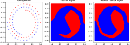
Figure 6: Comparison of standard training and polishing via geometric algebra in the spiral dataset.

4.1 Refining neural network weights via geometric algebra

We apply the characterization of Theorem 6, which states that the hidden neurons are scalar multiples of $\star(x_{j_{1}}\wedge\cdots\wedge x_{j_{r-1}})$, Additionally, they are orthogonal to the $r-1$ training data points specified by ${x_{j_{1}},\cdots,x_{j_{r-1}}}$, where $r$ represents the rank of the training data matrix.

The inherent challenge lies in identifying the specific subset of the $r-1$ training points needed to form each neuron. Fortunately, this subset can be estimated when we have access to approximate neuron weights, typically acquired using backpropagation-based stochastic gradient descent (SGD). After obtaining an approximate weight vector for each neuron, we can gauge which subsets of training data are nearly orthogonal to the neuron. This is achieved by evaluating the inner-products between the neuron weight and all training vectors, subsequently selecting the $r-1$ entries of the smallest magnitude. This refinement, which we term the polishing process, is delineated as follows for each neuron $w_{1},...,w_{m}$:
   For each $j\in[m]$

1. Calculate the inner-product magnitudes: $|x_{i}^{T}w_{j}|$ for each $i\in[n]$.

2. Identify the $r-1$ training vectors with the minimal inner-product magnitude, denoted as ${x_{j_{1}},\cdots,x_{j_{r-1}}}$.

3. Update the neuron using: $w_{j}\leftarrow\star(x_{j_{1}}\wedge\cdots\wedge x_{j_{r-1}})=\times(x_{j_{1}},\dots,x_{j_{r-1}})$. As a result, we have $w_{j}\perp x_{j_{1}},\dots,x_{j_{r-1}}$.

4. Optimize the weights of the following layer.

5. Optimize the scaling factor of the neuron (see Appendix 6.12).

To illustrate this method, we present two illustrative examples in Figures 6 and Figure 7.

Figure 6 for the 2D spiral dataset and a two-layer neural network optimized with squared loss. In the initial panel of this figure, the training curve of a two-layer ReLU neural network from (2) is depicted, considering $p=2$ and weight decay regularization set at $\beta=10^{-5}$. The dataset, divided into two classes represented by blue and red crosses, is showcased in the second panel. By resorting to the dual formulation in (5), the global optimum value is computed.Notably, while the gradient descent approach doesn’t closely approximate the global optimum, the polishing process enhances the neurons, leading to a marked improvement in the objective value—evidenced by the solid line in the left panel. A comparative visualization of the decision region pre and post-polishing is presented in the subsequent panels, highlighting the enhanced data distribution fit due to the polishing.

In Figure 7, we investigate binary image classification on the CIFAR-10 dataset [27]. On the left panel, a three-layer ReLU network is trained using SGD to differentiate between the ’automobile’ and ’ship’ labels. After a training duration of 10 epochs, we implement polishing on the first layer, following which the final layer of scalar weights is re-optimized. This procedure is executed with varying neuron counts in the second layer while the number of neurons in the first layer is fixed to 128, the learning rate of SGD is taken $0.01$ and the batch size is set to 32. The resulting average train/validation accuracies over 20 independent trials are plotted. The right panel demonstrates the effect of using different learning rates in the same setting when the initial two layers have 128 neurons. Polishing is applied to the second layer, post which the final scalar weight layer undergoes re-optimization. Notably, in both scenarios, a substantial enhancement in both training and validation accuracy is observed after polishing.

In both of the above cases, the optimization of the final layer of scalar weights is achieved by solving the regularized least squares problem, ensuring global optimality while the rest of the weights remain unchanged.

5 Discussion

In this work, we have presented an analysis that uncovers a deep connection between Clifford’s geometric algebra and optimal ReLU neural networks. By demonstrating that optimal weights of such networks are intrinsically tied to the wedge product of training samples, our results enable an understanding of how neural networks build representations as explicit functions of the training data points. Moreover, these closed-form functions not only provide a theoretical lens to understand the internal dynamics of neural networks, but also has the potential to guide new training algorithms that directly harness these geometric insights.

Our findings also contribute to the broader challenge of neural network interpretability. By elucidating the roles hidden layers play in encoding geometric information of training data points through signed volumes of shapes like triangles and parallelotopes, we have taken a step towards a more transparent and foundational theory of deep learning.

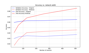
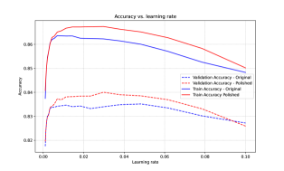
Figure 7: Comparison of standard training and polishing via geometric algebra in the CIFAR image classification benchmark.

We presented a numerical approach capitalizing on closed-form formulas to refine neural network parameters. This polishing process based on geometric algebra offers a promising avenue to improve the performance of neural networks while enabling their interpretability. These developments also underlines the potential and utility of integrating geometric algebra into the theory of deep learning.

There are many open questions for further research. Exploring how these insights apply to state-of-the-art network architectures, or in the context of different regularization techniques and variations of activation functions, such as the ones in attention layers, could be of significant interest. While our techniques allow for the interpretation of layer weights in popular pretrained network models, we leave this for further research. Additionally, practical implications of our results, including potential improvements to the polishing process remain to be fully explored.

6 Appendix

6.1 Generalized cross products

Definition 4.

Let $x_{1},\ldots,x_{d-1}\in\mathbb{R}^{d}$ be a collection of $d-1$ vectors and let $A=\begin{bmatrix}x_{1},\ldots,x_{d-1}\end{bmatrix}\in\mathbb{R}^{d\times(d-1)}$ be the matrix whose columns are the vectors $\{x_{i}\}_{i=1}^{d-1}$. The generalized cross product [28] of $x_{1},\ldots,x_{d-1}$ is defined as

$$x_{1}\times\ldots\times x_{d-1}=\times(x_{1},\ldots,x_{d-1})\triangleq\sum_{i=1}^{d}(-1)^{i-1}|A_{i}|e_{i},$$ (46)

where $A_{i}$ is the square matrix obtained from $A$ by deleting the $i$-th row and $\{e_{i}\}_{i}^{d}$ is the standard basis of $\mathbb{R}^{d}$.

We next list some properties of the generalized cross product.

• The cross product $\times(x_{1},\ldots,x_{d-1})$ is orthogonal to all vectors $x_{1},\ldots,x_{d-1}$.

• The cross product $\times(x_{1},\ldots,x_{d-1})$ equals zero if and only if $x_{1},\ldots,x_{d-1}$ are linearly dependent.

• The norm of the cross product is given by the $(d-1)$-volume of the parallelotope spanned by $x_{1},\ldots,x_{d-1}$, which is defined as

  $$P(x_{1},\ldots,x_{d-1})\triangleq\Big{\{}\sum_{i=1}^{d-1}t_{i}x_{i}\,|\,0\leq t_{i}\leq 1\,\forall i\in[d-1]\Big{\}},$$

  where $x_{1},\ldots,x_{d-1}$ are linearly independent.

• The cross product changes its sign when the order of two vectors is interchanged, i.e., $x_{1}\times x_{2}\times...\times x_{d}=-x_{2}\times x_{1}\times...\times x_{d}$ due to the determinant expansion of the cross product in (46).

• Inner-product with a vector gives the $d$-volume of the parallelotope spanned by $x_{1},\ldots,x_{d-1}$ and the vector, i.e.,

  $$\times(x_{1},\ldots,x_{d-1})^{T}x=\det\Big{[}x~{}~{}x_{1}~{}~{}\ldots~{}~{}x_{d-1}\Big{]}=\mathbf{Vol}\big{(}P(x,x_{1},\ldots,x_{d-1})\big{)}.$$

• Distance of a vector $x$ to the linear span of a collection of vectors $x_{1},...,x_{d-1}$ is given by

  $$\mathbf{dist}(x,\mathbf{Span}(x_{1},\ldots,x_{d-1}))=\frac{\mathbf{Vol}\big{(}P(x,x_{1},\ldots,x_{d-1})\big{)}}{\mathbf{Vol}\big{(}P(x_{1},\ldots,x_{d-1})\big{)}}=\frac{\times(x_{1},\ldots,x_{d-1})^{T}x}{\|\times(x_{1},\ldots,x_{d-1})\|_{2}}.$$

• Distance of a vector $x$ to the affine hull of a collection of vectors $x_{1},...,x_{d-1}$ is given by

  $$\mathbf{dist}(x,\mathbf{Aff}(x_{1},\ldots,x_{d-1}))=\frac{\mathbf{Vol}\big{(}P(x-x_{d},x_{1}-x_{d},\ldots,x_{d-1})\big{)}}{\mathbf{Vol}\big{(}P(x_{1}-x_{d},\ldots,x_{d-1}-x_{d})\big{)}}=\frac{\times(x_{1}-x_{d},\ldots,x_{d-1}-x_{d})^{T}(x-x_{d})}{\|\times(x_{1}-x_{d},\ldots,x_{d-1}-x_{d})\|_{2}}.$$

When $d=3$, the cross product reduces to the usual cross product of three vectors in $\mathbb{R}^{3}$. For example,

$$\begin{bmatrix}a\\ b\\ c\end{bmatrix}\times\begin{bmatrix}a^{\prime}\\ b^{\prime}\\ c^{\prime}\end{bmatrix}=\begin{bmatrix}bc^{\prime}-b^{\prime}c\\ ca^{\prime}-c^{\prime}a\\ ab^{\prime}-a^{\prime}b\end{bmatrix}.$$

When $d=2$, the cross product of a vector $\times x$ is rotation by a right angle in the clockwise direction in the plane. For example,

$$\times\Big{(}\begin{bmatrix}a\\ b\end{bmatrix}\Big{)}=\begin{bmatrix}b\\ -a\end{bmatrix}.$$

Detailed derivations of these results as well as further properties of generalized cross products can be found in Section 8.11 of [28], and their connections to the volumes of parallelotopes and zonotopes can be found in [29].

6.2 Proof of Theorem 1

Consider the dual constraint in (5), which can be rewritten as

$$\sup_{w,\,b\in\mathbb{R}\,:\,\|w\|_{p}\leq 1}|\sum_{i}v_{i}(x_{i}w+b)_{+}|\leq\lambda.$$ (47)

Since $w$ is a scalar, the constraint $\|w\|_{p}\leq 1$ is equivalent to $|w|\leq 1$ for all $p\in(0,\infty)$. An optimal $w$ satisfies $w\in\{-1,+1\}$ since either this constraint is tight or the objective is constant with respect to $w$. Next, observe that an optimal $b$ is achieved when $b\in\pm\{x_{i}\}_{i=1}^{n}$ or the objective goes to infinity when $\beta\rightarrow\infty$. This is because the objective is a piecewise linear function of $b$. In the latter case, the objective value is infinite as long as $\sum_{i}v_{i}\neq 0$. Therefore, we can rewrite (47) as

$$\max\Big{\{}|\sum_{i}v_{i}(x_{i}-x_{j})_{+}|,|\sum_{i}v_{i}(x_{j}-x_{i})_{+}|\Big{\}}\leq\lambda\quad\mbox{and}\quad\sum_{i}v_{i}=0$$ (48)

We use strong Lagrangian duality to obtain the claimed convex program using Lemma 21. It can be seen that the network given in (10) achieves the optimal objective on the training dataset since $f(X)=[f(x_{1}),\cdots,f(x_{n}))]^{T}=Kz^{*}+{1}t^{*}$.

6.3 Proof of Theorem 2 and Theorem 6

We now present the proof of Theorem 6, and the special case Theorem 2, which shows the equivalence of the $\ell_{1}$-regularized neural network and the Lasso problem in (30). Suppose that the training matrix is of rank $k$. Denote the compact Singular Value Decomposition (SVD) of ${X}$ as follows ${X}=U\Sigma V^{T}$ where $U\in\mathbb{R}^{n\times d}$ and $V\in\mathbb{R}^{d\times d}$ are orthonormal matrices and $\Sigma\in\mathbb{R}^{d\times d}$ is a diagonal matrix with non-negative diagonal entries. Only $k$ diagonal entries of $\Sigma$ are non-zero and the rest are zero. We denote the non-zero diagonal entries of $\Sigma$ as $\sigma_{1},\cdots,\sigma_{k}$ and the corresponding columns of $U$ and $V$ as $u_{1},\cdots,u_{k}$ and $v_{1},\cdots,v_{k}$, respectively.

Consider the NN objective (2). It can be seen that the projection $v_{i}^{T}W_{1j}$ of the hidden neuron weights $j\in[m]$ does not affect the objective value for $i=k+1,...,d$. Therefore, the optimal hidden weights are zero in the subspace $v_{k+1},...,v_{d}$ due to the norm regularization. In the remaining, we assume that the training matrix ${X}$ is full column rank and of size $n$ by $d=r$. Otherwise, we can remove the zero singular value subspaces of ${X}$ via the above argument.

We consider the convex dual of the $\ell_{1}$-regularized NN problem (30), and focus on the dual problem given in (5) when $\sigma$ is the ReLU activation function.

$$\max_{v\in\mathbb{R}^{n}}\,\,-\ell^{*}(v,y)\quad\mbox{s.t.}\quad\max_{w\,:\,\|w\|_{p}\leq 1}|v^{T}({X}w)_{+}|\leq\lambda.$$ (49)

The above optimization problem is a convex semi-infinite program which has a finite number of variables but infinitely many constraints. Our main strategy is to show that the constraint set can be described by a finite number of fixed points by analyzing the extreme points of certain convex subsets.

As shown in [8], the constraint $|v^{T}({X}w)_{+}|\leq\lambda$ can be analyzed by enumerating the hyperplane arrangement patterns

$$\{\mathrm{D}_{k}\}_{k=1}^{P}=\Big{\{}\mathrm{diag}(1[{X}w\geq 0])\,:w\in\mathbb{R}^{d}\Big{\}},$$

where $P$ is the number of distinct hyperplane arrangement patterns and $\mathrm{D}_{k}\in\{0,1\}^{n\times n}$ is the indicator matrix of the $k$-th pattern. The number $P$ is finite and satisfies the upper-bound by $P\leq 2\sum_{j=0}^{r-1}{n-1\choose j}$ where $r=\mathbf{rank}(X)$. Note that we have the identity

$$({X}w)_{+}=\mathrm{D}_{k}{X}w\quad\forall w\,:\mathrm{D}_{k}{X}w\geq 0,\,(\mathrm{I}-\mathrm{D}_{k}){X}w\leq 0\,,$$

which shows that the ReLU activation applied to the vector ${X}w$ can be expressed as a linear function whenever $w$ is in the cone $(2\mathrm{D}_{k}-\mathrm{I}){X}w\geq 0$. Using the above parameterization, we write the subproblem in the constraint of (49) when $p=1$ as follows

$$d_{\mathrm{sub}}\triangleq \max_{w}|v^{T}\mathrm{D}_{k}{X}w|$$ (50)

$$\mbox{s.t. }\|w\|_{1}\leq 1,\,(2\mathrm{D}_{k}-\mathrm{I}){X}w\geq 0.$$

We next claim that the constraint $\|w\|_{1}\leq 1$ is active at the optimum, assuming the objective value is positive. Note that $w=0$ is a feasible point, which achieves the objective value of zero. Otherwise, we can scale $w$ to satisfy the constraint and increase the objective value. Defining the set

$$\mathcal{C}\triangleq\left\{(2D_{i}-I)Xw\geq 0,\,\|w\|_{1}=1\right\},$$

we can express the dual subproblem $d_{\mathrm{sub}}$ using the set $\mathcal{C}$ as follows

$$d_{\mathrm{sub}}=\max\left\{0,\,\,\max_{w\in\mathcal{C}}v^{T}\mathrm{D}_{k}{X}w,\,\,\max_{w\in\mathcal{C}}-v^{T}\mathrm{D}_{k}{X}w\right\}.$$

Note that the maxima in the last two problems are achieved at extreme points of $\mathcal{C}$ since $\mathcal{C}$ is a bounded polytope and the objectives are linear functions.

The following lemma provides a characterization of the extreme points of the constraint set of the dual subproblem.

Lemma 14.

A vector $w$ is an extreme point of the set $\mathcal{C}$ if and only if $w\in\mathcal{C}$ and

$$\begin{bmatrix}{X}\\ \mathrm{I}\end{bmatrix}_{S}w=0\quad\mbox{and}\quad\|w\|_{1}=1$$ (51)

where $S$ is a subset of $d-1$ linearly independent rows of $\begin{bmatrix}{X}\\ \mathrm{I}\end{bmatrix}$.

We identify the extreme points via the cross product as follows. After defining the augmented data rows $x_{n+i}=e_{i}$ where $e_{i}$ is the $i$-th standard basis vector, a vector $w\in\mathcal{C}$ is an extreme point of $\mathcal{C}$ if $w\in\mathbf{Span}(\mathbin{\scalebox{1.15}{$\times$}}_{j\in S}x_{j})$ for some subset $S$ of size $d-1$ such that $\{x_{j}\}_{j\in S}$ are linearly independent and $\|w\|_{1}=1$. Since this span is a $d-1$ dimensional subspace, we can write $w$ as $\frac{\mathbin{\scalebox{1.15}{$\times$}}_{j\in S}x_{j}}{\big{\|}\mathbin{\scalebox{1.15}{$\times$}}_{j\in S}x_{j}\big{\|}_{1}}$. Note that the denominator is non-zero since $\{x_{j}\}_{j\in S}$ are linearly independent and $\|\mathbin{\scalebox{1.15}{$\times$}}_{j\in S}x_{j}\|_{1}\geq\|\mathbin{\scalebox{1.15}{$\times$}}_{j\in S}x_{j}\|_{2}$, which is the non-zero absolute volume of the parallelotope spanned by $\{x_{j}\}_{j\in S}$. Consecutively, we apply this characterization of extreme points to the expression for $d_{\mathrm{sub}}$ to obtain

$$d_{\mathrm{sub}}=\max\left\{0,\,\,\max_{w\in\mathcal{V}}v^{T}\mathrm{D}_{k}{X}w\right\},$$

where $\mathcal{V}\triangleq\Big{\{}\pm\frac{\mathbin{\scalebox{1.15}{$\times$}}_{j\in S}x_{j}}{\|\mathbin{\scalebox{1.15}{$\times$}}_{j\in S}x_{j}\|_{1}}\,:\,\{x_{j}\}_{j\in S}\mbox{ linearly independent},\,|S|=d-1\Big{\}}$.

Next we note that $\mathrm{D}_{k}{X}w=({X}w)_{+}$ for $w\in\mathcal{V}\subseteq\mathcal{C}$, which shows that the dual problem $d^{*}$ in (49) is equivalent to the following problem

$$\max_{v\in\mathbb{R}^{n}}\,\,-\ell^{*}(v,y)\quad\mbox{s.t.}\quad|v^{T}({X}w)_{+}|\leq\lambda\,\,\forall w\in\mathcal{V}.$$ (52)

By applying the characterization of the extreme points, we reduce the semi-infinite problem in (49) which has an infinite number of constraints to a problem with finite constraints.

Taking the Lagrangian dual of the above convex problem by introducing dual variables for each of the constraints, we arrive at the $\ell_{1}$ penalized convex problem

$$\min_{z}\,\,\ell(Kz,y)+\lambda\sum_{j}|z_{j}|.$$

Here, $K_{ij}=\Big{(}j_{0}x_{i}^{T}\frac{\mathbin{\scalebox{1.15}{$\times$}}(x_{j_{1}},...,x_{j_{d-1}})}{\|\mathbin{\scalebox{1.15}{$\times$}}(x_{j_{1}},...,x_{j_{d-1}})\|_{1}}\Big{)}_{+}=\frac{\big{(}j_{0}\mathbf{Vol}(\mathcal{P}(x_{j}\,:\,j\in S))\big{)}_{+}}{\|\mathbin{\scalebox{1.15}{$\times$}}(x_{j_{1}},...,x_{j_{d-1}})\|_{1}}$ using the multi-index notation $j=(j_{0},j_{1},...,j_{d-1})$ where $j_{0}$ ranges over $\{-1,+1\}$ to represent the choice of sign in the expression $\pm x_{i}^{T}\frac{\mathbin{\scalebox{1.15}{$\times$}}(x_{j_{1}},...,x_{j_{d-1}})}{\|\mathbin{\scalebox{1.15}{$\times$}}(x_{j_{1}},...,x_{j_{d-1}})\|_{1}}$. Rescaling the dual variables $z_{j}$ by $\|\mathbin{\scalebox{1.15}{$\times$}}(x_{j_{1}},...,x_{j_{d-1}})\|_{1}$, we obtain the problem

$$\min_{z}\,\,\ell(Kz,y)+\lambda\sum_{j}w_{j}|z_{j}|.$$

where $K_{ij}=\big{(}j_{0}\mathbf{Vol}(\mathcal{P}(x_{j_{1}},\,...,\,x_{j_{d-1}}))\big{)}_{+}$ and $w_{j}=\|\mathbin{\scalebox{1.15}{$\times$}}(x_{j_{1}},...,x_{j_{d-1}})\|_{1}$.

Finally, in order to simplify the notation, we take the index set $(j_{1},...,j_{d-1})$ over all subsets of $\{1,...,n\}$ of size $d-1$ and redefine the matrix as $K_{ij}=\mathbf{Vol}_{+}(\mathcal{P}(x_{j_{1}},\,...,\,x_{j_{d-1}}))$ and $w_{j}=\|\mathbin{\scalebox{1.15}{$\times$}}(x_{j_{1}},...,x_{j_{d-1}})\|_{1}$. This follows from the fact that the Euclidean norm of the cross-product, and hence the volume of the paralleltope is zero the whenever the subset of vectors are linearly dependent. Moreover, the index $j_{0}\in\{-1,+1\}$ is absorbed into the ordering of the vectors $x_{j_{1}},...,x_{j_{d-1}}$ in the parallelotope, by noting that the sign of the cross product is flipped whenever the ordering of two vectors is flipped. This completes the proof of Theorem 6.

Next, we provide the proofs of the lemmas used in the above proof.

Proof of Lemma 14.

We express $w=w^{+}-w^{-}$ where $w^{+}\geq 0$ and $w^{-}\geq 0$ represent the positive and negative part of $w$ respectively. Then, we express the extreme points of the set $\mathcal{C}$ using this lifted representation as follows

$$\mathcal{C}^{\prime}\triangleq\Bigg{\{}\begin{bmatrix}w^{+}\\ w^{-}\end{bmatrix}:\,(2D_{i}-I)(Xw^{+}-Xw^{-}) \geq 0,\,\,w_{+},w_{-}\geq 0,\ 1^{T}w^{+}+1^{T}w^{-}=1\Bigg{\}}.$$

We next argue that the extreme points of $\mathcal{C}$ can be analyzed via the extreme points of $\mathcal{C}^{\prime}$. In particular, it holds that

$$\max_{w\in\mathcal{C}}~{}x^{T}w=\max_{w\in\mathcal{C}^{\prime}}~{}x^{T}(w^{+}-w^{-})$$

for all $x\in\mathbb{R}^{d}$ and a maximizer $w$ to the former maximization problem can be obtained from a maximizer $(w^{+},w^{-})$ to the latter problem by setting $w^{*}=w^{+}-w^{-}$. On the other hand, a maximizer $(w^{+},w^{-})$ to the latter problem can be obtained from a maximizer $w$ to the former problem by setting $w^{+}=\max\{w,0\}$ and $w^{-}=\max\{-w,0\}$. Therefore, characterizing the extreme points of $\mathcal{C}$ is equivalent to characterizing the extreme points of $\mathcal{C}^{\prime}$.

This can be written in matrix notation as follows

$$\underbrace{\begin{bmatrix}(2D_{i}-I)X&-(2D_{i}-I)X\\ I&0\\ 0&I\\ \end{bmatrix}}_{M}\begin{bmatrix}w^{+}\\ w^{-}\\ \end{bmatrix}\geq 0\qquad\mbox{and}\qquad 1^{T}\begin{bmatrix}w^{+}\\ w^{-}\\ \end{bmatrix}=1.$$

Using Lemma 17, the extreme points of the above set are given by the unique solutions of the linear system

$$\begin{bmatrix}M_{S}\\ 1^{T}\end{bmatrix}\begin{bmatrix}w^{+}\\ w^{-}\\ \end{bmatrix}=\begin{bmatrix}0\\ 1\\ \end{bmatrix}$$

where $M_{S}$ is a submatrix of $M$ such that $\begin{bmatrix}M_{S}\\ 1^{T}\end{bmatrix}\in\mathbb{R}$ is full rank. For any extreme point $(w^{+},w^{-})$ of $\mathcal{C}^{\prime}$, the vector $w=w^{+}-w^{-}$ is an extreme point $\mathcal{C}$. It can be seen that at least $d$ coordinates of $\begin{bmatrix}w^{+}\\ w^{-}\\ \end{bmatrix}$ are zero since $w=w^{+}-w^{-}$ is the decomposition of $w$ into positive and negative parts. In order to characterize non-zero extreme points, we may assume that not all of the constraints $\begin{bmatrix}w^{+}\\ w^{-}\\ \end{bmatrix}\geq 0$ are active, since otherwise $w^{+}=w^{-}=0$ implying $w=0$. We next show that the rows of $M_{S}$ are linearly independent from the row vector $1^{T}$ due to the structure of $M$. Specifically, the top block $\begin{bmatrix}(2D_{i}-I)X&-(2D_{i}-I)X\end{bmatrix}$ has row span orthogonal to $1^{T}$, and the bottom block $\begin{bmatrix}I&0\\ 0&I\end{bmatrix}$ consists of canonical basis vectors, for which not all constraints are active (otherwise this implies $w=0$), which makes the subset of active rows linearly independent from $1^{T}$.

We conclude that the non-zero extreme points of $\mathcal{C}$ are given by $w=w^{+}-w^{-}\in\mathcal{C}$ such that

$$\begin{bmatrix}M_{S}\\ 1^{T}\end{bmatrix}\begin{bmatrix}w^{+}\\ w^{-}\\ \end{bmatrix}=\begin{bmatrix}0\\ 1\\ \end{bmatrix},$$

where $S$ is a subset of $2d-1$ linearly independent rows of $M$ and the above linear system has a unique solution. Recall that at least $d$ coordinates of $\begin{bmatrix}w^{+}\\ w^{-}\\ \end{bmatrix}$ are zero at any extreme point due to the decomposition $w=w^{+}-w^{-}$ where $w^{+}=(w)_{+}$ and $w^{-}=(w)_{-}$ are the positive and negative parts of $w$ respectively. Suppose that the vector $\begin{bmatrix}w^{+}\\ w^{-}\\ \end{bmatrix}$ is a non-zero extreme point and has $d+k$ zero entries for some $k\in\mathbb{Z}_{+}$, then $2d-1-(d+k)=d-1-k$ entries of $\begin{bmatrix}(2D_{i}-I)X&-(2D_{i}-I)X\end{bmatrix}\begin{bmatrix}w^{+}\\ w^{-}\\ \end{bmatrix}$ are zero. Mapping this decomposition back to the usual representation, this implies that an extreme point $w\in\mathcal{C}$ has $k$ zero entries and the vector $(2D_{i}-I)Xw$ has $d-1-k$ zero entries. Therefore, $d-1$ of the constraints $\begin{bmatrix}(2D_{i}-I)X\\ I\end{bmatrix}w\geq 0$ are active at a non-zero extreme point $w\in\mathcal{C}$. We conclude that $w\in\mathcal{C}$ is a non-zero extreme point of $\mathcal{C}$ if and only if

$$\begin{bmatrix}(2D_{i}-I)X\\ I\end{bmatrix}_{R}w=0\quad\mbox{and}\quad\|w\|_{1}=1,$$

where $R$ is a subset of $d-1$ linearly independent rows of the matrix $\begin{bmatrix}(2D_{i}-I)X\\ I\end{bmatrix}$. Finally, we observe that the constraint $\begin{bmatrix}(2D_{i}-I)X\\ I\end{bmatrix}_{R}w=0$ can be substituted by $\begin{bmatrix}X\\ I\end{bmatrix}_{R}w=0$ since $(2D_{i}-I)$ is a diagonal matrix containing $\pm 1$ values on the diagonal, and note that linear independence is invariant to this diagonal sign multiplication. ∎

6.4 Proof of Theorem 7

We now present the proof of Theorem 7 which shows the approximate equivalence of the $\ell_{2}$-regularized neural network and the Lasso problem in (34). We consider the dual problem in (5) and analyze its constraints, which are as follows:

$$\max_{i\in[P]}\max_{w}|v^{T}\mathrm{D}_{i}{X}w|\leq\lambda$$ (53)

$$\mbox{s.t. }\|w\|_{2}\leq 1,\,(2\mathrm{D}_{i}-\mathrm{I}){X}w\geq 0.$$

Here

$$\{\mathrm{D}_{i}\}_{i=1}^{P}=\Big{\{}\mathrm{diag}(1[{X}w\geq 0])\,:w\in\mathbb{R}^{d}\Big{\}},$$

are the diagonal hyperplane arrangement patterns.

As in Section 6.3, we assume that the training matrix ${X}$ is full column rank and of size $n$ by $d=r$, without loss of generality.

Consider the sub-problem arising in the above constraint given by

$$d^{+}_{sub}(i)\triangleq \max_{w}v^{T}D_{i}Xw$$

$$\mbox{s.t. }\|w\|_{2}\leq 1,\,(2D_{i}-I)Xw\geq 0.$$

We define the set

$$\mathcal{C}_{2}(i)\triangleq\Big{\{}w\,:\,\|w\|_{2}\leq 1,\,(2D_{i}-I)Xw\geq 0\Big{\}},$$

and let $d^{-}_{sub}(i)\triangleq\max_{w\in\mathcal{C}_{2}(i)}-v^{T}D_{i}Xw$. Note that the constraint in (5) is precisely $d^{+}_{sub}(i)\leq\lambda,\,d^{-}_{sub}(i)\leq\lambda~{}\forall i$. Our strategy is to show that $d^{+}_{sub}(i)$ and $d^{-}_{sub}(i)$ can be tightly approximated by a polyhedral approximation constructed using the extreme rays of the cone $\{w~{}:~{}(2D_{i}-I)Xw\geq 0\}$. Consequently, we will be able to obtain an approximation of the dual problem since the dual constraint is

$$d_{const}^{*} =\max_{i\in\{1,...,P\}}\max_{w\in\mathcal{C}_{2}}|v^{T}D_{i}Xw|=\max\Big{(}\max_{i\in\{1,...,P\}}d^{+}_{sub}(i),\max_{i\in\{1,...,P\}}d^{-}_{sub}(i)\Big{)}.$$ (54)

We first focus on a generic instance of the problem $d^{+}_{sub}=d^{+}_{sub}(i)$ and $\mathcal{C}_{2}=\mathcal{C}_{2}(i)$ for a certain value of $i$. Suppose that the extreme rays of the convex polyhedral cone

$$\{w\,:\,(2D_{i}-I)Xw\geq 0\}\subseteq\mathbb{R}^{d}$$

are $R_{1},...,R_{k}\subseteq\mathbb{R}^{d}$ for some $k\in\mathbb{Z}_{+}$. Note that by our assumption that $X$ is full column rank, this cone is pointed since it does not contain any nontrivial linear subspace. Let $p_{1},\ldots,p_{k}\in\mathbb{S}^{d-1}$ denote the unit norm generators of the extreme rays $R_{1},...,R_{k}$ normalized to unit Euclidean norm. We define the convex sets

$$\mathcal{P} \triangleq\mathbf{Conv}(p_{1},...,p_{k})\quad\mbox{and}\quad\mathcal{P}_{0}\triangleq\mathbf{Conv}(0,p_{1},...,p_{k}).$$

We will use the convex set $\mathcal{P}_{0}$ as an inner polyhedral approximation of $\mathcal{C}_{2}$. We define the distance of the convex set $\mathcal{P}$ from the origin as

$$d_{\min}\triangleq\mathbf{dist}(0,\mathcal{P})=\min_{w\in\mathcal{P}}\|w\|_{2}.$$

We have $d_{\min}\leq 1$ since $\|\sum_{i}\alpha_{i}p_{i}\|_{2}\leq\sum_{i}|\alpha_{i}|\|p_{i}\|_{2}=\sum_{i}|\alpha_{i}|=1$ for any $\alpha_{i}\geq 0$ and $\sum_{i}\alpha_{i}=1$, noting that $\|p_{i}\|_{2}=1$.

We apply Lemma 15 to obtain the following lower and upper bounds on $d^{+}_{sub}$:

$$\max_{w\in\mathcal{P}_{0}}v^{T}D_{k}Xw\ \leq\max_{w\in\mathcal{C}_{2}}v^{T}D_{k}Xw \leq\max_{w\in d_{\min}^{-1}\mathcal{P}_{0}}v^{T}D_{k}Xw$$ (55)

$$=d_{\min}^{-1}~{}\max_{w\in\mathcal{P}_{0}}v^{T}D_{k}Xw.$$

Next, we simplify the polyhedral approximation $\max_{w\in\mathcal{P}_{0}}v^{T}D_{k}Xw$. Applying Weyl’s Facet Lemma (see Lemma 19) to the cone $K=\{w\,:\,(2D_{i}-I)Xw\geq 0\}$, we see that a vector $v\in K$ belongs to an extreme ray of $K$ if and only if there are $d-1$ linearly independent rows of the matrix $(2D_{i}-I)X$ orthogonal to $v$. Then, each of the generators of the extreme rays $p_{1},...,p_{k}$ satisfy $p_{i}^{T}x_{j}=0,\,j\in S_{i}$ where $S_{i}$ is a subset of $d-1$ linearly independent rows of the matrix $X$. Using the properties of the generalized cross product (see 6.1), we identify each generator as a scalar multiple of the cross-product $\mathbin{\scalebox{1.15}{$\times$}}_{j\in S_{i}}x_{j}$ of the $d-1$ linearly independent rows $x_{j}$ of $X$. Note that the cross product of $d-1$ linearly independent vectors is orthogonal to each vector and lies on a one-dimensional linear subspace. Therefore the unit-norm vectors $p_{i}$ can be identified as $p_{i}=\pm\frac{\mathbin{\scalebox{1.15}{$\times$}}_{j\in S_{i}}x_{j}}{\|\mathbin{\scalebox{1.15}{$\times$}}_{j\in S_{i}}x_{j}\|_{2}}$, where the sign is chosen so that $p_{i}\in K$, i.e., $p_{i}^{T}D_{k,jj}x_{j}\geq 0$ for all $j\in S_{i}$.

Next, note that Weyl’s Facet Lemma also guarantees that any vector $p\in K$ of the form $p=\frac{\mathbin{\scalebox{1.15}{$\times$}}_{j\in S}x_{j}}{\|\mathbin{\scalebox{1.15}{$\times$}}_{j\in S}x_{j}\|_{2}}$ is on an extreme ray of $K$ when $S$ is a subset of $d-1$ linearly independent rows of $X$. When $d\geq 2$, the collection of vectors $0\cup\{\pm\mathbin{\scalebox{1.15}{$\times$}}_{j\in S}x_{j}\,:\,S\subseteq[n],~{}\dim\mathbf{Span}\{x_{j}:j\in S\}=d-1\}$ is equivalent to $0\cup\{\mathbin{\scalebox{1.15}{$\times$}}_{j\in S}x_{j}\,:\,S\subseteq P_{d-1}([n])\}$, where $P_{d-1}([n])$ denotes all permutations of subsets of $[n]$ with $d-1$ elements. In order to see this equivalence, observe that the $\pm 1$ multiplier can be removed when we consider permutations since exchanging the order of the two vectors in the cross product changes the sign of the resulting vector. Moreover, we can only consider subsets $S$ of size $d-1$, otherwise the vectors are linearly dependent and the cross product is zero. In addition, when the vectors are linearly dependent, the cross product is zero, which is already included in the collection of vectors.

Using this characterization, we can simplify the first optimization problem in (55) by enumerating all unit-norm generators of the extreme rays of the cone $K$, which can be done by considering all subsets $S$ of $d-1$ linearly independent rows of $X$ and taking the cross product of the rows in each subset. Define the set $\mathcal{D}_{S}$ as follows

$$\mathcal{D}_{S}=\Bigg{\{}\mathbin{\scalebox{1.15}{$\times$}}_{\begin{subarray}{c}j\in S\end{subarray}}x_{j}\Bigg{\}}\cup 0.$$

Then, we have

$$\max_{w\in\mathcal{P}_{0}}\,v^{T}D_{k}Xw=\max_{w\in\{0,p_{1},...,p_{k}\}}\,v^{T}D_{k}Xw=\max_{S\subseteq P_{d-1}([n])}\max_{\begin{subarray}{c}w\in K\cap\mathcal{D}_{S}\end{subarray}}\,v^{T}\Big{(}\frac{Xw}{\|w\|_{2}}\Big{)}_{+},$$ (56)

where the last maximization is over $d-1$ permutations $P_{d-1}([n])$ of subsets of $[n]$, and $w\in K\cap\mathcal{D}_{S}$. The justification of (56) is as follows: In the first equality in (56), we can drop the convex hull of $\{0,p_{1},...,p_{k}\}$ since the objective is linear. In the second equality, we replace the unit norm generators by their expressions given by the cross product and use the fact that $D_{i}Xw=(Xw)_{+}$ for $w\in K$. Note that the cross product is zero when the vectors are linearly dependent to simplify the expression of $\mathcal{D}_{S}$ in the last equality above.

Next, we plug-in the expression for $d^{+}_{sub}$ given in the last equality of (56) for $d^{+}_{sub}(i)$ in (54), repeat the same argument for $d^{-}_{sub}(i)$ which is identical, and use the approximation bound in (55)

$$d_{\mathrm{const}}^{*}~{} =~{}\max_{i\in\{1,...,P\},~{}s\in\{+1,-1\}}~{}~{}\max_{w\in\mathcal{C}_{2}(i)}sv^{T}D_{i}Xw$$ (57)

$$\leq d_{\min}^{-1}\max_{i\in\{1,...,P\},~{}s\in\{+1,-1\}}\max_{S\subseteq P_{d-1}([n])}\max_{\begin{subarray}{c}w\in K(i)\cap\mathcal{D}_{S}\end{subarray}}\,sv^{T}\Big{(}X\frac{w}{\|w\|_{2}}\Big{)}_{+}$$ (58)

where $K(i):=\{w~{}:~{}(2D_{i}-I)Xw\geq 0\}$. Noting that

$$\cup_{i=1}^{P}K(i)=\cup_{i=1}^{P}\{w~{}:~{}(2D_{i}-I)Xw\geq 0\}=\mathbb{R}^{d},$$

since the union of the chambers of the arrangement is the entire $d$-dimensional space, maximizing over the index $i\in\{1,...,P\}$ and $w\in K(i)\cap\mathcal{D}_{S}$ is equivalent to maximizing $w$ over $\cup_{i=1}^{P}K(i)\cap\mathcal{D}_{S}=\mathcal{D}_{S}$. Therefore, we obtain

$$\hat{d}\leq d_{\mathrm{const}}^{*} \leq d_{\min}^{-1}~{}\hat{d},$$ (59)

where

$$\hat{d}\triangleq\max_{S\subseteq P_{d-1}([n])}\max_{\begin{subarray}{c}w\in\mathcal{D}_{S}\end{subarray}}\,\Big{|}v^{T}\Big{(}X\frac{w}{\|w\|_{2}}\Big{)}_{+}\Big{|}.$$ (60)

Using the expression of the dual in (5), we have

$$p^{*}=\max_{d_{\mathrm{const}}^{*}(v)\leq\lambda}-\ell^{*}(v)$$ (61)

where $d_{\mathrm{const}}^{*}=d_{\mathrm{const}}^{*}(v)$ is as defined in (57). We then use the inequalities in (59) to get the lower and upper-bounds on the optimal objective as follows

$$\max_{d_{\min}^{-1}\hat{d}(v)\leq\lambda}-\ell^{*}(v)\leq p^{*}\leq\max_{\hat{d}(v)\leq\lambda}-\ell^{*}(v)\,,$$ (62)

where $\hat{d}(v)=\hat{d}$ is as defined in (60). Replacing the duals of the maximization problems in the above equation using Lemma 20, we obtain

$$\min_{z}\ell(\tilde{K}z,y)+d_{\min}\lambda\|z\|_{1}\leq p^{*}\leq\hat{p}_{\lambda}:=\min_{z}\ell(\tilde{K}z,y)+\lambda\|z\|_{1}\,.$$ (63)

Here, we defined $\hat{p}_{\lambda}$ as the optimal value of the Lasso objective and $\tilde{K}$ is the matrix defined as follows

$$K_{i,j}=x^{T}\frac{\times(x_{1},...,x_{d-1})}{\|\times(x_{1},...,x_{d-1})\|_{2}}\,,$$ (64)

where $j=(j_{1},...,j_{d})$ is a multi-index. The above shows that the optimal value $p^{*}$ corresponding to the NN objective in (1) when $p=2$ is bounded between the convex Lasso program in the right-hand side of (63) and the same convex program with a slightly smaller regularization coefficient as follows

$$\hat{p}_{d_{\min}\lambda}\leq p^{*}\leq\hat{p}_{\lambda}.$$

Noting that

$$\ell(\tilde{K}\hat{z}_{d_{\min}\lambda},y)+d_{\min}\lambda\|\hat{z}_{d_{\min}\lambda}\|_{1} \geq\min_{z}\ell(\tilde{K}z,y)+\lambda\|z\|_{1}+(d_{\min}-1)\lambda\|\hat{z}_{d_{\min}\lambda}\|_{1}$$

$$=\hat{p}_{\lambda}-(1-d_{\min})\lambda\|\hat{z}_{d_{\min}\lambda}\|_{1}\,,$$

where $\hat{z}_{d_{\min}\lambda}$ is a minimizer of the Lasso problem corresponding to $\hat{p}_{d_{\min}\lambda}$. we get the inequalities

$$\hat{p}_{\lambda}-(1-d_{\min})\|\hat{z}_{d_{\min}\lambda}\|_{1}\leq\hat{p}_{d_{\min}\lambda}\leq p^{*}\leq\hat{p}_{\lambda}\,.$$ (65)

This shows that the optimality gap is at most $(1-d_{\min})\lambda\|\hat{z}_{d_{\min}\lambda}\|_{1}$, where $\hat{z}_{d_{\min}\lambda}$ is an optimal solution of the Lasso problem in the left-hand side of (63) with regularization coefficient $d_{\min}\lambda$.

We now obtain upper and lower-bounds on $\hat{p}_{\lambda}$ in terms of $p^{*}$ by noting that (59) implies

$$d^{*}_{\mathrm{const}}\leq d_{\min}^{-1}\hat{d}\leq d_{\min}^{-1}d^{*}_{\mathrm{const}}.$$

Multiplying both sides by $d_{\min}$ we obtain

$$d_{\min}d^{*}_{\mathrm{const}}\leq\hat{d}\leq d^{*}_{\mathrm{const}}.$$

Using the above inequalities in the dual programs, we get

$$\max_{d^{*}(v)\leq\lambda}-\ell^{*}(v)\leq\max_{\hat{d}(v)\leq\lambda}-\ell^{*}(v)\leq\max_{d_{\min}d^{*}_{\mathrm{const}}(v)\leq\lambda}-\ell^{*}(v).$$ (66)

Using the dual of the Lasso program again from Lemma (5), we obtain

$$p^{*}\leq\min_{z}\ell(\tilde{K}z,y)+\lambda\|z\|_{1}\leq p^{*}_{d^{-1}_{\min}\lambda}~{},$$ (67)

where $p^{*}_{\lambda^{\prime}}$ in the right-hand side is defined as

$$p^{*}_{\lambda^{\prime}}\triangleq\min_{{W}_{1},{W}_{2}}\ell\Big{(}\sum_{j=1}^{m}\sigma({X}{W}_{1j}+{1}b_{1j}){W}_{2j},y\Big{)}+\lambda^{\prime}\sum_{j=1}^{m}\|{W}_{1j}\|_{2}^{2}+\|{W}_{2j}\|_{2}^{2},$$ (68)

for $m\geq m^{*}$ where $m^{*}$ is the number of neurons in an optimal solution of the bidual of (49) when $p=2$. Here, $p^{*}_{d_{\min}^{-1}\lambda}$ is the value of the optimal NN objective when the regularization coefficient is set to to the larger value $d_{\min}^{-1}\lambda$. This value can be upper-bounded as follows

$$p^{*}_{d_{\min}^{-1}\lambda} \leq F({W}_{1}^{*},{W}_{2}^{*})+d_{\min}^{-1}\lambda R({W}_{1}^{*},{W}_{2}^{*})$$ (69)

$$=F({W}_{1}^{*},{W}_{2}^{*})+\lambda R({W}_{1}^{*},{W}_{2}^{*})+(d_{\min}^{-1}-1)\lambda R({W}_{1}^{*},{W}_{2}^{*})$$ (70)

$$=p^{*}_{\lambda}+(d_{\min}^{-1}-1)\lambda R({W}_{1}^{*},{W}_{2}^{*})\,,$$ (71)

where $F(\cdot,\cdot)$ and $R(\cdot,\cdot)$ are the functions in the first (loss) and second (regularization) terms in the objective (68) respectively, and $({W}_{1}^{*},{W}_{2}^{*})$ is an optimal solution of (68), i.e., we have $p^{*}_{\lambda}=F({W}_{1}^{*},{W}_{2}^{*})+\lambda R({W}_{1}^{*},{W}_{2}^{*})$. Therefore, (67) implies that

$$p^{*}\leq\min_{z}\ell(\tilde{K}z,y)+\lambda\|z\|_{1}\leq p^{*}+(d_{\min}^{-1}-1)\lambda R({W}_{1}^{*},{W}_{2}^{*})\leq d_{\min}^{-1}p^{*}\,,$$ (72)

where $R({W}_{1}^{*},{W}_{2}^{*}):=\sum_{j=1}^{m}\|{W}^{*}_{1j}\|_{2}^{2}+\|{W}^{*}_{2j}\|_{2}^{2}$ is the regularization term corresponding to any optimal solution of (68). The final inequality follows from $\lambda R({W}_{1}^{*},{W}_{2}^{*})\leq p^{*}$. This shows that the optimality gap of the Lasso solution is at most $\frac{1-d_{\min}}{d_{\min}}\lambda R({W}_{1}^{*},{W}_{2}^{*})$.

Finally, to simplify the expression of the matrix $\tilde{K}$ given in (64), we use the following cross-product representation of the distance to an affine hull (see Appendix)

$$x^{T}\frac{\times(x_{1},...,x_{d-1})}{\|\times(x_{1},...,x_{d-1})\|_{2}} =\mathbf{dist}(x,\mathbf{Aff}(0,x_{1},...,x_{d-1}))$$

$$=\mathbf{dist}(x,\mathbf{Span}(x_{1},...,x_{d-1}))\,,$$

for any $x,x_{1},...,x_{d-1}\in\mathbb{R}^{d}$ where $\times(x_{1},...,x_{d-1})$ is the cross product of the vectors $x_{1},...,x_{d-1}$. Combining the bounds (65) and (72) with the lower bound on the minimum distance $d_{\min}$ in terms of the maximum chamber diameter $r$ from Lemma 16 completes the proof.

6.5 Proof of Theorem 23

The proof parallels the proof of Theorems 6 and 7. Here, we only highlight the main differences.

The convex dual of the problem (94) is given by

$$p_{v}^{*}\geq d_{v}^{*}\triangleq\max_{V\in\mathbb{R}^{n}}\,\,-\ell^{*}(V,Y)\quad\mbox{s.t.}\quad\|V^{T}\sigma({X}w)\|_{2}\leq\lambda,\,\forall w\in\mathcal{B}_{p}^{d}.$$ (73)

This dual convex program was derived in [30], where it was also shown that strong duality holds if the number of neurons, $m$, exceed the critical threshold $m^{*}$, which is the number of neurons in the convex bidual program.

We focus on the dual constraint subproblem in (73) given by

$$d_{\mathrm{v-sub}}\triangleq \max_{w}\|V^{T}\mathrm{D}_{k}{X}w\|_{2}$$

$$\mbox{s.t. }\|w\|_{p}\leq 1,\,(2\mathrm{D}_{k}-\mathrm{I}){X}w\geq 0.$$

$$= \max_{w}\max_{u:~{}\|u\|_{2}\leq 1}|u^{T}V^{T}\mathrm{D}_{k}{X}w|$$

$$\mbox{s.t. }\|w\|_{p}\leq 1,\,(2\mathrm{D}_{k}-\mathrm{I}){X}w\geq 0.$$

We note that the above problem has the same form of equation (50) and (53) for $p=1$ and $p=2$ respectively, where the vector $v$ plays the role of $Vu$. The rest of the proof is identical for both cases. ∎

Figure 8: Illustration of the Archimedean approximation in Lemma 15.

Lemma 15 (Archimedean approximation of spherical sections via polytopes).

Suppose that $\mathbf{Cone}(P)\cap-\mathbf{Cone}(P)=\{0\}$, i.e., $\mathbf{Cone}(P)$ does not contain a non-trivial (non-zero dimensional) linear subspace. Then, it holds that

$$\mathcal{P}_{0}\subseteq\mathcal{C}_{2}\subseteq d_{\min}^{-1}\mathcal{P}_{0}.$$

Proof.

The first inclusion follows by noting that $\mathcal{P}_{0}$ is a polytope and it is contained in $\mathcal{C}_{2}$ since all of its extreme points $0,p_{1},...,p_{k}$ are contained in the convex set $\mathcal{C}_{2}$.

In order to prove the second inclusion, we first show that $\mathcal{C}_{2}=\mathbf{Cone}(P)\cap\{\|w\|_{2}\leq 1\}$. Since $\mathbf{Cone}(P)$ is pointed, i.e., $\mathbf{Cone}(P)\cap-\mathbf{Cone}(P)=\{0\}$, it is equal to the convex hull of its extreme rays (Theorem 13 of [31]). Since the extreme rays of $\mathbf{Cone}(P)$ are the extreme rays of the cone $\{w\,:\,(2D_{i}-I)Xw\geq 0\}$, are identical and the latter cone is also pointed, these two cones are identical. Therefore, we have $\mathcal{C}_{2}=\mathbf{Cone}(P)\cap\{\|w\|_{2}\leq 1\}$.

Next, suppose that there exists some $w^{*}\in\mathcal{C}_{2}$. Then, $\exists t\in\mathbb{R}_{+},\alpha_{i}\geq 0,\sum_{i}\alpha_{i}=1$ such that $w^{*}=t\sum_{i}\alpha_{i}p_{i}$ since $w^{*}\in\mathbf{Cone}(P)$. Since $\|w^{*}\|_{2}\leq 1$, we have $1\geq\|w^{*}\|_{2}=\|t\sum_{i}\alpha_{i}p_{i}\|_{2}\geq t\min_{\alpha_{i}}\|\sum_{i}\alpha_{i}p_{i}\|_{2}\geq t\min_{w\in\mathcal{P}}\|w\|_{2}=t\,d_{\min}$. From this chain of inequalities, we obtain the upper-bound $t\leq d_{\min}^{-1}$. We have $w^{*}\in d_{\min}^{-1}\mathcal{P}_{0}$ since

$$w^{*}=t\sum_{i}\alpha_{i}p_{i}\in t\mathbf{Conv}(p_{1},...,p_{k})\in\mathbf{Conv}(0,p_{1},...,p_{k})\in d_{\min}^{-1}\mathcal{P}_{0}.$$

∎

Lemma 16 (Diameter of a chamber bounds its distance to the origin).

Consider the set $\tilde{\mathcal{C}_{2}}:\{w\,:\,(2D_{i}-I){X}w\geq 0,\,\|w\|_{2}=1\}$. Suppose that $r\in\mathbb{R}$ is the $\ell_{2}$-diameter of $\tilde{\mathcal{C}_{2}}$, which is defined as the smallest $r\geq 0$ such that $\|w_{1}-w_{2}\|_{2}\leq r$ for all $w_{1},w_{2}\in\tilde{\mathcal{C}_{2}}$. Then,

$$d_{\min}:=\min_{v\in\mathbf{Conv}(v_{1},...,v_{k})}\|v\|_{2}\geq 1-r,$$

for any set of $k$ vectors $\{v_{1},...,v_{k}\}\in\tilde{\mathcal{C}_{2}}$.

Proof.

Since the $\ell_{2}$-diameter of the set $\tilde{\mathcal{C}_{2}}$ is upper bounded by $r$, we first argue that there exists a Euclidean ball of radius $r$ that contains $\tilde{\mathcal{C}_{2}}$ as follows. Suppose that $w_{1},w_{2}$ are two vectors in $\tilde{\mathcal{C}_{2}}$ that achieve the $\ell_{2}$-diameter $r$, i.e., $\|w_{1}-w_{2}\|_{2}=r$. Then, the Euclidean ball of radius $r$ centered at $\frac{w_{1}+w_{2}}{2}$ contains $\tilde{\mathcal{C}_{2}}$ since for all $w\in\tilde{\mathcal{C}_{2}}$ it holds that

$$\|w-\frac{w_{1}+w_{2}}{2}\|_{2}=\frac{1}{2}\|(w-w_{1})+(w-w_{2})\|_{2}\leq\frac{1}{2}\|w-w_{1}\|_{2}+\frac{1}{2}\|w-w_{2}\|\leq r.$$

Next, note that $\mathbf{Conv}(v_{1},...,v_{k})$ is contained in this ball due to the convexity of the Euclidean ball and since $v_{1},...,v_{k}\in\tilde{\mathcal{C}_{2}}$ are contained in this set. Therefore, the minimum norm point

$$v^{*}:=\arg\min_{v\in\mathbf{Conv}(v_{1},...,v_{k})}\|v\|_{2},$$

satisfies $\|v^{*}\|\geq\|v_{1}\|_{2}-\|v^{*}-v_{1}\|_{2}=1-\|v^{*}-v_{1}\|_{2}\geq 1-r$. ∎

Proof of Lemma 12.

We use Lemma 2.1 of [23] by taking $K$ equal to the unit Euclidean sphere in $\mathbb{R}^{d}$. Since the Gaussian width of this set is bounded by $\sqrt{d}$, Lemma 2.1 implies that

$$\Big{|}\frac{1}{m}\|Xz\|_{1}-\alpha\Big{|}\leq\varepsilon\quad\forall z~{}:~{}\|z\|_{2}=1,$$

with probability at least $1-2e^{-nu^{2}/2}$, where $\alpha=\sqrt{2/\pi}$ and $\varepsilon=4\sqrt{\frac{d}{n}}+u$. Rewriting the above inequality as $-\varepsilon\leq\frac{1}{m}\|X\frac{w}{\|w\|_{2}}\|_{1}-\alpha\leq\varepsilon~{}\forall w$, multiplying each side by $\|w\|_{2}$ and letting $u=\sqrt{\frac{d}{n}}$, we observe that the $\ell_{1}$ isometry condition (44) where $\epsilon=5\sqrt{\frac{d}{n}}$ holds with probability at least $1-2e^{-d/2}$. Invoking Lemma 11, we obtain that the maximum chamber radius is bounded by $4\sqrt{\epsilon}=4\sqrt{5\sqrt{\frac{d}{n}}}\leq 9(\frac{d}{n})^{1/4}$, which concludes the proof. ∎

Proof of Lemma 11.

Suppose that $w_{1},w_{2}\in\tilde{\mathcal{C}_{2}}$. Then, $w_{a}:=\frac{1}{2}(w_{1}+w_{2})$ satisfies $(2D_{i}-I){X}w_{a}\geq 0$ since $w_{1},w_{2}$ belongs to the set $(2D_{i}-I){X}w\geq 0$, which is convex. Therefore, we have

$$|x_{i}^{T}w_{a}| =\frac{1}{2}|x_{i}^{T}w_{1}+x_{i}^{T}w_{2}|$$

$$=\frac{1}{2}\mathrm{sign}(x_{i}^{T}w_{1}+x_{i}^{T}w_{2})(x_{i}^{T}w_{1}+x_{i}^{T}w_{2})$$

$$=\frac{1}{2}\Big{(}\mathrm{sign}(x_{i}^{T}w_{1})(x_{i}^{T}w_{1})+\mathrm{sign}(x_{i}^{T}w_{2})(x_{i}^{T}w_{2})\Big{)}$$

$$=\frac{1}{2}|x_{i}^{T}w_{1}|+\frac{1}{2}|x_{i}^{T}w_{2}|.$$

where the third equality follows since $\textrm{sign}(x_{i}^{T}w_{1})=\textrm{sign}(x_{i}^{T}w_{2})\,\forall i$ due to the constraints $(2D_{i}-I){X}w_{1}\geq 0$ and $(2D_{i}-I){X}w_{2}\geq 0$. Note that since $\|Xw\|_{1}=\sum_{i=1}^{n}|x_{i}^{T}w|$, this implies the identity

$$\|Xw_{a}\|_{1}=\frac{1}{2}\|Xw_{1}\|_{1}+\frac{1}{2}\|Xw_{2}\|_{1}.$$

Applying the isometry condition given in (44) to $w_{a}$ and using the above identity, we get

$$\alpha(1+\epsilon)\|w_{a}\|_{2} \geq\frac{1}{n}\|Xw_{a}\|_{1}$$

$$=\frac{1}{2n}\|Xw_{1}\|_{1}+\frac{1}{2n}\|Xw_{2}\|_{1}$$

$$\geq\frac{1}{2}\alpha(1-\epsilon)\|w_{1}\|_{2}+\frac{1}{2}\alpha(1-\epsilon)\|w_{2}\|_{2}$$ (74)

$$=\alpha(1-\epsilon)\,,$$

where the inequality (74) follows from the concentration inequality (44) applied to $w_{1}$ and $w_{2}$. Therefore, we have $\|w_{a}\|_{2}\geq(1+\epsilon)^{-1}(1-\epsilon)$ and

$$\|w_{a}\|_{2}^{2}=\big{\|}\frac{1}{2}(w_{1}+w_{2})\big{\|}_{2}^{2}=\frac{1}{2}+\frac{w_{1}^{T}w_{2}}{2} \geq\Big{(}\frac{1-\epsilon}{1+\epsilon}\Big{)}^{2}\geq 1-4\epsilon\,.$$

The last inequality holds since

$$(1-\epsilon^{2})=1-2\epsilon+\epsilon^{2}\geq 1-3\epsilon-4\epsilon^{2}=(1+\epsilon)(1-4\epsilon)\,,$$

for $\epsilon\geq 0$. This implies $w_{1}^{T}w_{2}\geq 1-8\epsilon$. Since $w_{1}$ and $w_{2}$ are unit Euclidean norm, we get $\|w_{1}-w_{2}\|_{2}^{2}=2-2w_{1}^{T}w_{2}\leq 16\epsilon$. Therefore $\|w_{1}-w_{2}\|_{2}\leq 4\sqrt{\epsilon}$.

∎

6.6 Proofs for two-dimensional networks

Proof of Theorem 4.

The proof follows by specializing the proof of Theorem 7 to $d=2$ and noting that the chamber diameter is controlled by the angle $\epsilon\pi$. Consider the triangle corresponding the the chamber where the angular dispersion bound is achieved. Consider the bisector of this angle and observe that the chamber diameter is equal to $2\sin(\epsilon\pi/2)$, which is upper-bounded by $\epsilon\pi$. Although this provides the approximation factor $1/(1-\epsilon\pi)$ as long as $\epsilon<\pi^{-1}$, we can improve this bound by considering a direct Archimedean approximation of the circular section as shown in Figure 8 to replace Lemma (15). Specifically, using the bisector of the angle we also have

$$\mathcal{P}_{0}\subseteq\mathcal{C}_{2}\subseteq(\cos(\epsilon\pi/2))^{-1}\mathcal{P}_{0},$$

which improves Lemma (15). Finally, note that

$$(\cos(\epsilon\pi/2))^{-1}\leq 1+\epsilon~{},$$

for $\epsilon\in[0,1/2]$, which completes the proof. ∎

Proof sketch of Theorem 5.

The proof follows the same steps as in Theorem 4 except that we use the form of the dual program with bias terms given in Theorem 22. ∎

6.7 Proofs for deep neural networks

Proof of Theorem 9.

Suppose that an optimal solution of (42) is given by

$$\theta^{*}=\big{(}W^{*(1)},\cdots,W^{*(L)}\big{)}.$$

Define optimal activations of the first two-layer block based on the optimal $W^{*(1)},W^{*(2)}$ above as the matrix $Y^{{}^{*}(1)}$ by defining

$$Y^{{}^{*}(1)}:=\sigma(XW^{*(1)})W^{*(2)}.$$

Now, we focus on the first two-layer NN block and consider the following auxiliary problem

$$(\hat{W}^{(1)},\hat{W}^{(2)})=\arg\min_{W_{1}^{(1)},W_{2}^{(2)}}~{}\sum_{j=1}^{m}\|{W}^{(1)}_{\cdot j}\|_{p}^{2}+\|{W}^{(2)}_{j\cdot}\|_{p}^{2}$$ (75)

$$\mbox{s.t.}\qquad\sigma(XW^{(1)})W^{(2)}=Y^{{}^{*}(1)}.$$

The above problem is in the form of a two-layer neural network optimization problem. We now show that $\hat{W}^{(1)},\hat{W}^{(2)}$ combined with the rest of the optimal weights $W^{*(3)},W^{*(4)}\cdots,W^{*(L)}$ are also optimal in the optimization problem (42). First, note that the outputs of the network, $f_{\theta^{*}}(X)$ and $f_{\hat{\theta}_{1}}(X)$, are identical where $\theta^{*}$ is an optimal solution and

$$\hat{\theta}_{1}:=\big{(}\hat{W}^{(1)},\hat{W}^{(2)},W^{*(3)},W^{*(4)}\cdots,W^{*(L)}\big{)},$$

since the activations of the first two-layer block are identical. Second, note that the regularization terms $R_{\theta}^{(1)}:=\sum_{j=1}^{m}\|{W}^{(1)}_{\cdot j}\|_{p}^{2}+\|{W}^{(2)}_{j\cdot}\|_{p}^{2}$ are also equal since $R_{\hat{\theta}_{1}}^{(1)}<R_{\theta^{*}}^{(1)}$ contradicts the optimality of $\theta^{*}$ in (42) and $R_{\hat{\theta}_{1}}^{(1)}>R_{\theta^{*}}^{(1)}$ contradicts the optimality of $(\hat{W}^{(1)},\hat{W}^{(2)})$ in (75).

Next, we analyze the remaining layers. We define the optimal activations before and after the $\ell$-th two-layer NN block as follows

$$X^{*\ell} =\sigma(\cdots\sigma(XW^{*(1)})W^{*(2)}\cdots W^{*(\ell-1)})$$

$$Y^{*\ell} =\sigma(\cdots\sigma(XW^{*(1)})W^{*(2)}\cdots W^{*(\ell-1)})W^{*(\ell+1)}.$$

Consider the auxiliary problem for the $\ell$-th two-layer block

$$(\hat{W}^{(\ell)},\hat{W}^{(\ell+1)})=\arg\min_{W^{(\ell)},W^{(\ell+1)}}~{}\sum_{j=1}^{m}\|{W}^{(\ell)}_{\cdot j}\|_{p}^{2}+\|{W}^{(\ell+1)}_{j\cdot}\|_{p}^{2}$$ (76)

$$\mbox{s.t.}\qquad\sigma(X^{*\ell}W^{(\ell)})W^{(\ell+1)}=Y^{{}^{*}(\ell)}.$$

We show that $\hat{\theta}_{\ell}:=\big{(}W^{*(1)},W^{*(2)},\cdots\hat{W}^{(\ell)},\hat{W}^{(\ell+1)}\cdots,W^{*(L-1)},W^{*(L)}\big{)}$, which equals $\theta^{*}$ optimal in (42) except the $\ell$-th and $(\ell+1)$-th layer weights are replaced with an optimal solution of (76), is an optimal solution of (42). As in the above case, the outputs of the network, $f_{\theta^{*}}(X)$ and $f_{\hat{\theta}_{\ell}}(X)$, are identical by construction. Moreover, the regularization terms $R_{\theta}^{(\ell)}:=\sum_{j=1}^{m}\|{W}^{(\ell)}_{\cdot j}\|_{p}^{2}+\|{W}^{(\ell+1)}_{j\cdot}\|_{p}^{2}$ are also equal since $R_{\hat{\theta}_{\ell}}^{(\ell)}<R_{\theta^{*}}^{(\ell)}$ contradicts the optimality of $\theta^{*}$ in (42) and $R_{\hat{\theta}_{\ell}}^{(\ell)}>R_{\theta^{*}}^{(\ell)}$ contradicts the optimality of $(\hat{W}^{(\ell)},\hat{W}^{(\ell+1)})$ in (76) since $(\hat{W}^{(\ell)},\hat{W}^{(\ell+1)})$ is feasible in (76), i.e., $\sigma(X^{*\ell}W^{*(\ell)})W^{*(\ell+1)}=Y^{{}^{*}(\ell)}$.

Finally, we finish the proof by iteratively applying the above claims to invoke the two-layer result given in Theorem 23. Given an optimal solution $\theta^{*}$ of (42), we replace the first two-layer NN block with $(\hat{W}^{(1)},\hat{W}^{(2)})$ from (75) while maintaining global optimality with respect to (42). For $\ell=2,3,...,L$ we repeat this process in pairs of consecutive layers to reach the claimed result. ∎

Proof of Theorem 10.

The proof proceeds similar to the proof of Theorem 9. We first show that given an optimal solution $\theta^{*}$, we can replace the first two layers $(W^{*(1)},W^{*(2)})$ with $(\hat{W}^{(1)},\hat{W}^{(2)})$, where

$$(\hat{W}^{(1)},\hat{W}^{(2)})=\arg\min_{W_{1}^{(1)},W_{2}^{(2)}}~{}\sum_{j=1}^{m}\|{W}^{(1)}_{\cdot j}\|_{2}^{2}+\|{W}^{(2)}_{j\cdot}\|_{2}^{2}$$ (77)

$$\mbox{s.t.}\qquad\sigma(XW^{(1)})W^{(2)}=Y^{{}^{*}(1)},$$

and $Y^{{}^{*}(1)}:=\sigma(XW^{*(1)})W^{*(2)}$. By Corollary 8, the weights $(\hat{W}^{(1)},\hat{W}^{(2)})$ only increase the regularization $\sum_{j=1}^{m}\|{W}^{(1)}_{\cdot j}\|_{2}^{2}+\|{W}^{(2)}_{j\cdot}\|_{2}^{2}$ by a factor of $1/(1-\mathscr{D}(X))$, while producing the identical network output $f_{\hat{\theta}}(X)=f_{\theta^{*}}(X)$.

Next, we analyze the remaining layers one by one. We define the optimal activations before and after the $\ell$-th two-layer NN block as follows

$$X^{*\ell} =\sigma(\cdots\sigma(XW^{*(1)})W^{*(2)}\cdots W^{*(\ell-1)})$$

$$Y^{*\ell} =\sigma(\cdots\sigma(XW^{*(1)})W^{*(2)}\cdots W^{*(\ell-1)})W^{*(\ell+1)}.$$

Consider the auxiliary problem for the $\ell$-th two-layer block

$$(\hat{W}^{(\ell)},\hat{W}^{(\ell+1)})=\arg\min_{W^{(\ell)},W^{(\ell+1)}}~{}\sum_{j=1}^{m}\|{W}^{(\ell)}_{\cdot j}\|_{2}^{2}+\|{W}^{(\ell+1)}_{j\cdot}\|_{2}^{2}$$ (78)

$$\mbox{s.t.}\qquad\sigma(X^{*\ell}W^{(\ell)})W^{(\ell+1)}=Y^{{}^{*}(\ell)}.$$

By Theorem 23, replacing the weights $\hat{W}^{(\ell)},\hat{W}^{(\ell+1)}$ only increases the regularization term for those weights by a factor of $1/(1-\mathscr{D}(X^{*\ell}))$ while maintaining the network output $f_{\hat{\theta}}(X)=f_{\theta^{*}}(X)$. We can repeat this process for all $\ell=2,3,...,L$ one by one, i.e., replacing layers $1$ and $2$, $2$ and $3$,…. (as opposed to pairs of consecutive weights as in the proof of Theorem 9), we replace all the weights by increasing the total regularization term by a factor of at most $2/(1-\epsilon)$ assuming $\mathscr{D}(X)\leq\epsilon$ and $\mathscr{D}(X^{*\ell})\leq\epsilon$ for $\ell\in\{1,...,L-2\}$. The factor $2$ is needed to account for the overlapping weights in the replacement process. ∎

6.8 Proof of Theorem 3 and Theorem 22

We only highlight the differences from the proof of Theorem 6 in the proof below. The dual problem in (5) when an additional bias term is present takes the form

$$p^{*}\geq d^{*}\triangleq\max_{v\in\mathbb{R}^{n}}\,\,-\ell^{*}(v,y)\quad\mbox{s.t.}\quad|v^{T}\sigma({X}w+1b)|\leq\lambda,\,\forall w\in\mathcal{B}_{p}^{d},\,b\in\mathbb{R}.$$ (79)

As in the proof of Theorem 1, we focus on the dual constraint subproblem

$$\sup_{w\in\mathcal{B}_{p}^{d},\,b\in\mathbb{R}}\,|v^{T}\sigma({X}w+1b)|\leq\lambda$$ (80)

and observe that the above objective is piecewise linear in $b$. Moreover, the objective tends to infinity as $b\rightarrow\infty$ as long as $\sum_{i}v_{i}\neq 0$. Otherwise, an optimal choice for $b$ is $-x_{j}^{T}w^{*}$ for some index $j\in[n]$ for some optimal $w^{*}$.

Therefore, the constraint (80) can be rewritten as two constraints:

$$\max_{j\in[n]}\,\sup_{w\in\mathcal{B}_{p}^{d}}\,|\sum_{i}v_{i}\sigma((x_{i}-x_{j})^{T}w^{*})|\leq\lambda\quad\mbox{and}\quad\sum_{i}v_{i}=0.$$ (81)

The rest of the proof uses the same steps that follows (50) and the form of the Lasso with a bias term given in Lemma 21. ∎

6.9 Additional Lemmas

Lemma 17 (Extreme points of polytopes restricted to an affine set).

Suppose that $A\in\mathbb{R}^{n\times d}$, $b\in\mathbb{R}^{b}$, $c\in\mathbb{R}^{d}$ and $d\in\mathbb{R}$ are given. A vector $x\in\mathbb{R}^{d}$ is an extreme point of $\mathcal{C}\triangleq\left\{Ax\leq b,c^{T}x=d\right\}$ if and only if there exists a subset $S$ of $n$ linearly independent rows of $A$ such that $x$ is the unique solution of the linear system

$$\begin{bmatrix}A_{S}\\ c^{T}\end{bmatrix}x=\begin{bmatrix}0\\ d\end{bmatrix},$$ (82)

where the matrix $\begin{bmatrix}A_{S}\\ c^{T}\end{bmatrix}\in\mathbb{R}^{d\times d}$ is full rank. Here, $A_{S}\in\mathbb{R}^{d-1\times d}$ is the submatrix of $A$ obtained by selecting the $d-1$ rows indexed by $S$.

Proof.

We first provide a proof of the first direction (extreme point $\implies$ full rank) by contradiction. Let $x^{*}$ be an extreme point of $C$. We define $S$ as the subset of inequality constraints active at $x^{*}$ and $S^{c}$ as the subset of inequality constraints inactive. More precisely, we have $A_{S}x^{*}=0$ and $A_{S^{c}}x^{*}<0$ for some subset $S$ of $n$ rows of $A$ and its complement $S^{c}$. Suppose that the matrix $\begin{bmatrix}A_{S}\\ c^{T}\end{bmatrix}\in\mathbb{R}^{d\times d}$ is not full rank. Then we may pick $v\neq 0$ in the nullspace of this matrix. Define $x_{1}\triangleq x^{*}+\epsilon v$ and $x_{2}\triangleq x^{*}-\epsilon v$, which are feasible for $\mathcal{C}$ for any sufficiently small $\epsilon>0$ since $\begin{bmatrix}A_{S}\\ c^{T}\end{bmatrix}v=0$ and $A_{S^{c}}x^{*}<0$. However, this is a contradiction since $\frac{1}{2}x_{1}+\frac{1}{2}x_{2}=x^{*}$ and $x_{1},x_{2}\neq x^{*}$ implies that $x^{*}$ is not an extreme point of $\mathcal{C}$.

We next provide a proof of the second direction (full rank $\implies$ extreme point) by contradiction. Suppose that $x^{*}\in\mathcal{C}$ is a point such that $A_{S}x^{*}=0$ and $A_{S^{c}}x^{*}<0$ for some subset $S$ its complement $S^{c}$, $c^{T}x^{*}=d$, and the matrix $\begin{bmatrix}A_{S}\\ c^{T}\end{bmatrix}\in\mathbb{R}^{d\times d}$ is full row rank. It follows that $x^{*}$ is the unique solution of the linear system $\begin{bmatrix}A_{S}\\ c^{T}\end{bmatrix}x=\begin{bmatrix}0\\ d\end{bmatrix}$. We will show that $x^{*}$ is an extreme point. Suppose that this is not the case and there exists $x_{1},x_{2}\in\mathcal{C}$ distinct from $x^{*}$ such that $x^{*}=\frac{1}{2}x_{1}+\frac{1}{2}x_{2}$. Then, we have $Ax_{1}\leq 0$, $Ax_{2}\leq 0$ and $\frac{1}{2}A_{S}x_{1}+\frac{1}{2}A_{S}x_{2}=0$. Note that $A_{S}x_{1}\leq 0$ and $A_{S}x_{2}\leq 0$ together with $\frac{1}{2}A_{S}x_{1}+\frac{1}{2}A_{S}x_{2}=0$ imply that $A_{S}x_{1}=A_{S}x_{2}=0$ (In order to see this, suppose that $a_{j}^{T}x_{1}<0$ for some row $a_{j}$ of $A$ such that $j\in S$. Then we have $\frac{1}{2}a_{j}^{T}x_{1}+\frac{1}{2}a_{j}^{T}x_{2}<0$ which is a contradiction.). Finally, noting $c^{T}x_{1}=c^{T}x_{2}=d$ implies that $\begin{bmatrix}A_{S}\\ c^{T}\end{bmatrix}x_{1}=\begin{bmatrix}0\\ b\end{bmatrix}$ and $\begin{bmatrix}A_{S}\\ c^{T}\end{bmatrix}x_{2}=\begin{bmatrix}0\\ b\end{bmatrix}$, which is a contradiction since $x^{*}$ is the unique solution of this linear system. ∎

Lemma 18 (Rank reduction).

Let us denote the Singular Value Decomposition (SVD) of $X$ as $X=U\Sigma V^{T}$ in compact form, where $U\in\mathbb{R}^{n\times r}$, $\Sigma\in\mathbb{R}^{r\times r}$ and $V\in\mathbb{R}^{r\times d}$ and let $X=[U~{}U^{\perp}]\begin{bmatrix}\Sigma&0\\ 0&0\end{bmatrix}[V~{}V^{\perp}]^{T}$ denote the full SVD of $X$. Then, the following optimization problems are equivalent

$$p^{*}_{2}=\min_{{W}^{(1)},{W}^{(2)},b}\ell\Big{(}\sum_{j=1}^{m}\sigma({X}{W}^{(1)}_{j}){W}^{(2)}_{j},y\Big{)}+\lambda\sum_{j=1}^{m}\|{W}^{(1)}_{j}\|_{2}^{2}+\|{W}^{(2)}_{j}\|_{2}^{2},$$ (83)

$$p^{r}_{2}=\min_{\tilde{W}^{(1)},\tilde{W}^{(2)},b}\ell\Big{(}\sum_{j=1}^{m}\sigma(U\Sigma\tilde{W}^{(1)}_{j})\tilde{W}^{(2)}_{j},y\Big{)}+\lambda\sum_{j=1}^{m}\|\tilde{W}^{(1)}_{j}\|_{2}^{2}+\|\tilde{W}^{(2)}_{j}\|_{2}^{2},$$ (84)

i.e., $p^{*}=p^{r}$. Optimal solutions of (83) and (84) satisfy $(V^{\perp})^{T}W_{j}^{(1)}=0$, $V^{T}{W}^{(1)}_{j}=\tilde{W}^{(1)}_{j}$ and $W^{(2)}_{j}=\tilde{W}^{(2)}_{j}$ $\,\forall j\in[m]$.

Proof of Lemma 18.

We define $[\tilde{W}_{j}^{(1)}\hat{W}_{j}^{(1)}]\triangleq[V~{}V^{\perp}]W_{j}^{(1)}$ and plug-in the compact SVD of $X$ in the expression (83)

$$\min_{{W}^{(1)},{W}^{(2)},b}\ell\Big{(}\sum_{j=1}^{m}\sigma(U\Sigma\tilde{W}^{(1)}_{j}){W}^{(2)}_{j},y\Big{)}+\lambda\sum_{j=1}^{m}\|\tilde{W}^{(1)}_{j}\|_{2}^{2}+\|\hat{W}^{(1)}_{j}\|_{2}^{2}+\|{W}^{(2)}_{j}\|_{2}^{2},$$ (85)

where we have $\|W_{j}^{(1)}\|_{2}^{2}=\|[V~{}V^{\perp}]W_{j}^{(1)}\|_{2}^{2}=\|\tilde{W}_{j}^{(1)}\|_{2}^{2}+\|\hat{W}_{j}^{(1)}\|_{2}^{2}$. It can be seen that $\hat{W}_{j}^{(1)}=0~{}\forall j$ and $V^{T}{W}^{(1)}_{j}=\tilde{W}^{(1)}_{j}~{}\forall j$. ∎

6.10 Extreme rays of convex cones

In this subsection, we present some definitions and lemmas related to extreme rays of convex cones [31, 32].

Definition 5 (Rays).

Let $K$ be a convex cone in $\mathbb{R}^{d}$. A cone $R\subseteq K$ is called a ray of $K$ if $R=\{\lambda x\,:\,\lambda\geq 0\}$, for some $x\in K$.

Definition 6 (Extreme rays).

Let $K$ be a convex cone in $\mathbb{R}^{d}$. A ray $R=\{\lambda x\,:\,\lambda\geq 0\}\subseteq K$ generated by some vector $x$ is called an extreme ray of $K$ if $x$ is not a positive linear combination of two linearly independent vectors of $K$.

Lemma 19 (Weyl’s Facet Lemma [32]).

Define the convex cone $K=\{w\in\mathbb{R}^{d}\,:\,w^{T}p_{i}\leq 0,\,i\in[k]\}\subseteq\mathbb{R}^{d}$, where $p_{1},...,p_{k}\in\mathbb{R}^{d}$ are a collection of vectors. Then, a non-zero vector $x\in K$ is an element of an extreme ray of $K$ if and only if $\dim\mathbf{Span}(p_{i}\,:\,x^{T}p_{i}=0,\,i\in[k])=d-1$.

6.11 Duality and approximate duality

Lemma 20 (Dual of Lasso).

Suppose that $K\in\mathbb{R}^{n\times P}$ is a matrix whose columns are given by the vectors $k_{1},...,k_{p}\in\mathbb{R}^{n}$ and $\lambda>0$ is a regularization parameter. Then, the primal and dual optimization problems for Lasso are given by

$$\min_{z}\ell(Kz,y)+\lambda\|z\|_{1}~{}=~{}\max_{v~{}:~{}|v^{T}k_{j}|\leq\lambda\,\forall j\in[p]}-\ell^{*}(v)$$ (86)

Lemma 21 (Dual of Lasso with a bias term).

Consider the problem in Lemma 20 with an additional bias term. Then, the primal and dual optimization problems for Lasso are given by

$$\min_{z,\,b}\ell(Kz+1b,y)+\lambda\|z\|_{1}~{}=~{}\max_{\begin{subarray}{c}v~{}:~{}|v^{T}k_{j}|\leq\lambda\,\forall j\in[p]\\ \sum_{i}v_{i}=0\end{subarray}}-\ell^{*}(v)$$ (87)

Proof.

Lemma 20 and 21 are based on a standard application of Lagrangian duality [20]. Strong duality holds, i.e., the primal and dual problems have the same value which are both achieved, in both problems since $v=0$ in the dual problem is strictly feasible for the inequalities due to $\lambda>0$. ∎

6.12 Optimizing scaling coefficients

Our characterization of the hidden neurons using geometric algebra in Theorem 6 and 7 determine the direction of optimal neurons. The magnitude of the optimal neuron can be analytically determined. In this section, we show that the optimal scaling coefficients are given by the ratio of the norms of the corresponding weights.

Consider the two-layer neural network training problem given below

$$p^{*} \triangleq\min_{{W}^{(1)},{W}^{(2)},b}\ell\Big{(}\sum_{j=1}^{m}\sigma({X}{W}^{(1)}_{j}+{1}b_{j}){W}^{(2)}_{j},y\Big{)}+\lambda\sum_{j=1}^{m}\|{W}^{(1)}_{j}\|_{p}^{2}+\|{W}^{(2)}_{j}\|_{p}^{2},$$ (88)

where the activation function is positively homogeneous, i.e., $\sigma(\alpha x)=\alpha\sigma(x)$ for $\alpha>0$. Introducing non-negative scaling coefficients $\alpha_{1},...,\alpha_{m}$ to scale hidden neuron weight and bias, and dividing the corresponding second layer weight by the same scalar we obtain

$$p^{*} \triangleq\min_{\begin{subarray}{c}{W}^{(1)},{W}^{(2)},b\\ \alpha_{1},...,\alpha_{m}\geq 0\end{subarray}}\ell\Big{(}\sum_{j=1}^{m}\sigma({X}{W}^{(1)}_{j}\alpha_{j}+{1}b_{j}\alpha_{j}){W}^{(2)}_{j}\alpha_{j}^{-1},y\Big{)}+\lambda\sum_{j=1}^{m}\|{W}^{(1)}_{j}\|_{p}^{2}\alpha_{j}^{2}+\|{W}^{(2)}_{j}\|_{p}^{2}\alpha_{j}^{-2},$$ (89)

$$=\min_{\begin{subarray}{c}{W}^{(1)},{W}^{(2)},b\\ \alpha_{1},...,\alpha_{m}\geq 0\end{subarray}}\ell\Big{(}\sum_{j=1}^{m}\sigma({X}{W}^{(1)}_{j}+{1}b_{j}){W}^{(2)}_{j},y\Big{)}+\lambda\sum_{j=1}^{m}\|{W}^{(1)}_{j}\|_{p}^{2}\alpha_{j}^{2}+\|{W}^{(2)}_{j}\|_{p}^{2}\alpha_{j}^{-2},$$ (90)

where the last equality follows from the fact that $\sigma(\alpha x)=\alpha\sigma(x)$ for $\alpha>0$. Through simple differentiation, it is straightforward show that the optimal scaling coefficients are given by

$$\alpha_{j}^{*}=\Big{(}\frac{\|{W}^{(2)}_{j}\|_{p}}{\|{W}^{(1)}_{j}\|_{p}}\Big{)}^{1/2}~{}\mbox{for}~{}j\in[m].$$ (91)

6.13 Variations of the network architecture

6.13.1 Network weights with biases

Theorem 22.

The 2-layer neural network problem in (2) when $p=2$ and with trainable unregularized biases is equivalent to the following convex Lasso problem

$$\min_{z}\ell\big{(}Kz,y\big{)}+\lambda\sum_{j}|z_{j}|.$$ (92)

The matrix $K$ is defined as

$$K_{ij} =\frac{\big{(}(x_{i}-x_{r})\wedge(x_{j_{1}}-x_{j_{r}})\wedge\cdots\wedge(x_{j_{r-1}}-x_{j_{r}})\big{)}_{+}}{\|(x_{j_{1}}-x_{j_{r}})\wedge\,...\,\wedge(x_{j_{r-1}}-x_{j_{r}})\|_{2}}=\mathbf{dist}_{+}\big{(}x_{i},\,\mathbf{Aff}(x_{j_{1}},\,...,\,x_{j_{r-1}})\big{)}\,,$$

where the multi-index $j=(j_{1},...,j_{r})$ is over all combinations of $r$ rows of ${X}\in\mathbb{R}^{n\times d}$, and $r=\mathbf{rank}(X)$.

The proof of this theorem can be found in Subsection 6.8.

6.13.2 Vector-output Neural Networks

Consider the vector-output neural network problem in (2) given by

$$p_{v}^{*} \triangleq\min_{{W}^{(1)},{W}^{(2)},b}\ell\Big{(}\sum_{j=1}^{m}\sigma({X}{W}^{(1)}_{j}+{1}b_{j}){W}^{(2)}_{j},Y\Big{)}+\lambda\sum_{j=1}^{m}\|{W}^{(1)}_{j}\|_{p}^{2}+\|{W}^{(2)}_{j}\|_{p}^{2}.$$ (93)

Here, the matrix $Y\in\mathbb{R}^{n\times c}$ contains the $c$-dimensional training labels, and ${W}^{(1)}\in\mathbb{R}^{d\times m}$, ${W}^{(2)}\in\mathbb{R}^{m\times c}$, and $b\in\mathbb{R}^{m}$ are trainable weights. We have the following extension of the convex progam (30) for vector-output neural networks.

$$\hat{p}_{v}\triangleq\min_{Z\in\mathbb{R}^{p\times c}}\ell\big{(}KZ,Y\big{)}+\lambda\sum_{j=1}\|Z_{\cdot j}\|_{2},$$ (94)

where $Z_{j}$ is the $j$-th column of the matrix $Z$.

Theorem 23.

Define the matrix $K$ as follows

$$K_{ij}=\frac{\big{(}x_{i}\wedge x_{j_{1}}\wedge\cdots\wedge x_{j_{r-1}}\big{)}_{+}}{\|x_{j_{1}}\wedge\,...\,\wedge x_{j_{r-1}}\|_{p}}\,,$$

where the multi-index $j=(j_{1},...,j_{r-1})$ is over all combinations of $r$ rows and $r=\mathbf{rank}({X})$. It holds that

• when $p=1$, the convex problem (94) is equivalent to the non-convex problem (93), i.e., $p_{v}^{*}=\hat{p}_{v}$.

• when $p=2$, the convex problem (94) is a $\frac{1}{1-\epsilon}$ approximation of the non-convex problem (93), i.e., $p_{v}^{*}\leq\hat{p}_{v}\leq\frac{1}{1-\epsilon}p_{v}^{*}$, where $\epsilon\in(0,1)$ is an upper-bound on the maximum chamber diameter $\mathscr{D}({X})$.

An neural network achieving the above approximation bound can be constructed as follows:

$$f(x)=\sum_{j}Z^{*}_{\cdot j}\frac{\big{(}x_{i}\wedge x_{j_{1}}\wedge\cdots\wedge x_{j_{r-1}}\big{)}_{+}}{\|x_{j_{1}}\wedge\,...\,\wedge x_{j_{r-1}}\|_{p}}\,,$$ (95)

where $Z^{*}$ is an optimal solution to (94).

References

- Krizhevsky et al. [2012] Alex Krizhevsky, Ilya Sutskever, and Geoffrey E Hinton. Imagenet classification with deep convolutional neural networks. Advances in neural information processing systems, 25, 2012.
- LeCun et al. [2015] Yann LeCun, Yoshua Bengio, and Geoffrey Hinton. Deep learning. nature, 521(7553):436–444, 2015.
- OpenAI [2023] R OpenAI. Gpt-4 technical report. arXiv, pages 2303–08774, 2023.
- Papyan et al. [2020] Vardan Papyan, XY Han, and David L Donoho. Prevalence of neural collapse during the terminal phase of deep learning training. Proceedings of the National Academy of Sciences, 117(40):24652–24663, 2020.
- Jacot et al. [2018] Arthur Jacot, Franck Gabriel, and Clément Hongler. Neural tangent kernel: Convergence and generalization in neural networks. Advances in neural information processing systems, 31, 2018.
- Chizat et al. [2019] Lenaic Chizat, Edouard Oyallon, and Francis Bach. On lazy training in differentiable programming. Advances in neural information processing systems, 32, 2019.
- Radhakrishnan et al. [2023] Adityanarayanan Radhakrishnan, Mikhail Belkin, and Caroline Uhler. Wide and deep neural networks achieve consistency for classification. Proceedings of the National Academy of Sciences, 120(14):e2208779120, 2023.
- Pilanci and Ergen [2020] Mert Pilanci and Tolga Ergen. Neural networks are convex regularizers: Exact polynomial-time convex optimization formulations for two-layer networks. In International Conference on Machine Learning, pages 7695–7705. PMLR, 2020.
- Ergen and Pilanci [2021a] Tolga Ergen and Mert Pilanci. Convex geometry and duality of over-parameterized neural networks. The Journal of Machine Learning Research, 22(1):9646–9708, 2021a.
- Bartan and Pilanci [2021] Burak Bartan and Mert Pilanci. Training quantized neural networks to global optimality via semidefinite programming. In International Conference on Machine Learning, pages 694–704. PMLR, 2021.
- Ergen and Pilanci [2021b] Tolga Ergen and Mert Pilanci. Revealing the structure of deep neural networks via convex duality. In International Conference on Machine Learning, pages 3004–3014. PMLR, 2021b.
- Ergen and Pilanci [2021c] Tolga Ergen and Mert Pilanci. Global optimality beyond two layers: Training deep relu networks via convex programs. In International Conference on Machine Learning, pages 2993–3003. PMLR, 2021c.
- Wang and Pilanci [2022] Yifei Wang and Mert Pilanci. The convex geometry of backpropagation: Neural network gradient flows converge to extreme points of the dual convex program. In International Conference on Learning Representations, 2022.
- Wang et al. [2021] Yifei Wang, Jonathan Lacotte, and Mert Pilanci. The hidden convex optimization landscape of regularized two-layer relu networks: an exact characterization of optimal solutions. In International Conference on Learning Representations, 2021.
- Ergen et al. [2022a] Tolga Ergen, Arda Sahiner, Batu Ozturkler, John Pauly, Morteza Mardani, and Mert Pilanci. Demystifying batch normalization in relu networks: Equivalent convex optimization models and implicit regularization. International Conference on Learning Representations, 2022a.
- Lacotte and Pilanci [2020] Jonathan Lacotte and Mert Pilanci. All local minima are global for two-layer relu neural networks: The hidden convex optimization landscape. arXiv e-prints, 2020.
- Artin [2016] Emil Artin. Geometric algebra. Courier Dover Publications, 2016.
- Doran and Lasenby [2003] Chris Doran and Anthony Lasenby. Geometric algebra for physicists. Cambridge University Press, 2003.
- Dorst et al. [2012] Leo Dorst, Chris Doran, and Joan Lasenby. Applications of geometric algebra in computer science and engineering. Springer Science & Business Media, 2012.
- Boyd and Vandenberghe [2004] Stephen P Boyd and Lieven Vandenberghe. Convex optimization. Cambridge university press, 2004.
- Ergen et al. [2022b] Tolga Ergen, Halil Ibrahim Gulluk, Jonathan Lacotte, and Mert Pilanci. Globally optimal training of neural networks with threshold activation functions. In The Eleventh International Conference on Learning Representations, 2022b.
- Zeger et al. [2023] Emi Zeger, Yifei Wang, Mishkin Aaron, Tolga Ergen, Emmanuel Jean Candes, and Mert Pilanci. Neural networks for low dimensional data are convex lasso models. Technical Report, Stanford University, CA, USA, 2023.
- Plan and Vershynin [2014] Yaniv Plan and Roman Vershynin. Dimension reduction by random hyperplane tessellations. Discrete & Computational Geometry, 51(2):438–461, 2014.
- Gordon [1985] Yehoram Gordon. Some inequalities for gaussian processes and applications. Israel Journal of Mathematics, 50:265–289, 1985.
- Dvoretzky [1959] Aryeh Dvoretzky. A theorem on convex bodies and applications to banach spaces. Proceedings of the National Academy of Sciences, 45(2):223–226, 1959.
- Vershynin [2011] Roman Vershynin. Lectures in geometric functional analysis. Unpublished manuscript. Available at http://www-personal. umich. edu/romanv/papers/GFA-book/GFA-book. pdf, 3(3):3–3, 2011.
- Krizhevsky and Hinton [2009] Alex Krizhevsky and Geoffrey Hinton. Learning multiple layers of features from tiny images. Master’s thesis, University of Toronto, ON, Canada, 2009.
- Berger [2009] Marcel Berger. Geometry I. Springer Science & Business Media, 2009.
- Gover and Krikorian [2010] Eugene Gover and Nishan Krikorian. Determinants and the volumes of parallelotopes and zonotopes. Linear Algebra and its Applications, 433(1):28–40, 2010.
- Sahiner et al. [2020] Arda Sahiner, Tolga Ergen, John M Pauly, and Mert Pilanci. Vector-output relu neural network problems are copositive programs: Convex analysis of two layer networks and polynomial-time algorithms. In International Conference on Learning Representations, 2020.
- Fenchel and Blackett [1953] Werner Fenchel and Donald W Blackett. Convex cones, sets, and functions. Princeton University, Department of Mathematics, Logistics Research Project, 1953.
- Weyl [1950] Hermann Weyl. The elementary theory of convex polyhedra. Contributions to the Theory of Games, page 3, 1950.