Spin Drude weight for the integrable XXZ chain
with arbitrary spin

Abstract

Using generalized hydrodynamics (GHD), we exactly evaluate the finite-temperature spin Drude weight at zero magnetic field for the integrable XXZ chain with arbitrary spin and easy-plane anisotropy. First, we construct the fusion hierarchy of the quantum transfer matrices ($T$-functions) and derive functional relations ($T$- and $Y$-systems) satisfied by the $T$-functions and certain combinations of them ($Y$-functions). Through analytical arguments, the $Y$-system is reduced to a set of non-linear integral equations, equivalent to the thermodynamic Bethe ansatz (TBA) equations. Then, employing GHD, we calculate the spin Drude weight at arbitrary finite temperatures. As a result, a characteristic fractal-like structure of the Drude weight is observed at arbitrary spin, similar to the spin-1/2 case. In our approach, the solutions to the TBA equations (i.e., the $Y$-functions) can be explicitly written in terms of the $T$-functions, thus allowing for a systematic calculation of the high-temperature limit of the Drude weight.

1 Introduction

Quantum integrable systems are characterized by an infinite number of local or quasi-local conserved charges, which have led to extensive investigations into their unique physical properties. While conventional systems are understood through Gibbs ensembles, integrable systems, due to their multitude of extensive conserved charges, are described by Generalized Gibbs Ensembles (GGE) [1, 2] (refer to [3] for a review). This distinction becomes particularly evident in thermalization processes, where integrable systems often deviate from the predictions of frameworks like the eigenstate thermalization hypothesis [4].

On the other hand, our understanding of non-equilibrium properties in integrable systems has seen rapid advancements, largely attributed to the theoretical framework of Generalized Hydrodynamics (GHD) [5, 6] (see also [7] for lecture notes). GHD effectively merges the concepts of fluid mechanics and GGE, providing a novel perspective in studying the non-equilibrium properties of quantum integrable systems (recent reviews are available in [8, 9, 10]). Moreover, the GHD framework has been extended to weakly broken integrable systems (refer to [11, 12] for a review).

Among these advancements, the finite-temperature spin transport properties of the spin-1/2 XXZ chain, which are deeply relevant to this work, have been extensively studied for a considerable period [13]. The spin-1/2 XXZ chain is given by

$$\mathcal{H}_{0}=\frac{J}{4}\sum_{j=1}^{L}\left[\sigma_{j}^{x}\sigma_{j+1}^{x}+\sigma_{j}^{y}\sigma_{j+1}^{y}+\Delta\left(\sigma_{j}^{z}\sigma^{z}_{j+1}+1\right)\right],$$ (1.1)

where $\sigma_{j}^{x}$, $\sigma_{j}^{y}$, and $\sigma_{j}^{z}$ are the spin-1/2 spin operators (Pauli matrices), and $\Delta$ stands for the anisotropy parameter. In this model, the spin current is not a conserved quantity except for $\Delta=0$, which corresponds to a free fermion system. For $|\Delta|<1$, the system exhibits ballistic spin transport, characterized by a finite spin Drude weight [14, 15, 16, 17] and also by a dynamical exponent $z=1$ that signifies a scaling relation $x\sim t^{1/z}=t$ between the magnetization displacement $x$ and time $t$. In contrast, when $\Delta>1$, the spin transport is believed to be diffusive with a dynamical exponent $z=2$ [18, 19]. Interestingly, at the isotropic point $\Delta=1$, i.e., at the boundary between the diffusive and ballistic regimes, the spin transport at infinite temperature is considered to exhibit superdiffusive behavior with a dynamical exponent $z=3/2$ [18, 20, 21]. Further investigations [22] suggest that, particularly at this isotropic point, the transport properties are likely to belong to the Kardar-Parisi-Zhang (KPZ) universality class [23]. On the other hand, a recent investigation [24] indicates that the transport at $\Delta=1$ cannot be explained by the KPZ type, which has also been supported by recent quantum simulations [25]. From this perspective, the topic continues to be a subject of ongoing debate. More rigorous and quantitative analysis of spin transport at the isotropic point is desired, especially a more accurate evaluation of the exponent.

For $|\Delta=\cos(\pi/p_{0})|<1$, the spin Drude weight at finite temperatures had long been a topic of debate since Zotos derived it in [14] by combining Kohn’s formula [26] with the Thermodynamic Bethe Ansatz (TBA) [27]. Taking a notably different approach, Prosen and Ilievski evaluated the Drude weight at infinite temperature [15]. Specifically, they constructed quasi-local conserved charges and optimized the Mazur bound of the Drude weight using them. Remarkably, this optimized lower bound, referred to as the Prosen-Ilievski bound, exhibits a fractal-like structure, more aptly described as popcorn-like [28]. Moreover, with the emergence of GHD, the spin Drude weight has been formulated in a universal manner in [29, 30]. The result from GHD reproduces Zotos’s formula. Intriguingly, the high-temperature limit of the Drude weight exactly coincides with the Prosen-Ilievski bound [16]. This popcorn structure is intrinsically linked to the structures of strings [27] that define the thermodynamics of the XXZ model. In fact, recent studies suggest that similar popcorn structures also appear in higher-spin integrable XXZ models and the sine-Gordon model [28, 31, 32], where these thermodynamics are governed by the same strings as in the XXZ model.

This paper focuses on the finite-temperature spin Drude weight at zero magnetic field for an integrable XXZ chain with arbitrary spin $S$. We investigate the model in the critical regime, characterized by the anisotropy parameter $\Delta=\cos(\pi/p_{0})$ where $p_{0}\in\mathbb{Q}_{\geq 2}$. This model was introduced by Kirillov and Reshetikhin [33] through a “fusion” of the XXZ model. For $S=1$, the model corresponds to the Zamolodchikov-Fateev model [34]. Regarding the spin Drude weight, a suboptimal Mazur bound was derived for the high-temperature limit in the $S=1$ case [35]. More recently, the exact high-temperature behavior of this quantity has been further clarified for the specific case where $S=1$ and $p_{0}\in\mathbb{N}_{\geq 2}$ [28].

As reported in [33, 36], for $S\geq 1$, the anisotropy $\Delta$ must be constrained by the value of $S$ to ensure that the Hamiltonian derived from the fusion procedure possesses real eigenvalues. Specifically, for an integer spin $S$ greater than $2$, the permissible region of $\Delta$ is composed of several separate open intervals. This also holds for half odd integer spin $S$ greater than $7/2$. (See Table 1 in the main text.) Importantly, the low-energy properties in each region, for a given $S$, are governed by a distinct conformal field theory [36, 37]. From this perspective, it is crucial to delve into how this rich phase structure affects the transport properties.

We investigate the spin Drude weight of this model using GHD across a broad range of temperatures and anisotropies. To systematically derive the exact expressions at infinite temperature, we derive the TBA equations using the quantum transfer matrices (QTMs) and their functional relations referred to as the $T$ and $Y$-systems [38]. Notably, the resulting Drude weight, at both finite and infinite temperatures, prominently displays a popcorn structure that depends on $\Delta$ and exhibits discontinuities throughout. As expected from the different excitation properties in each region explained earlier, the behavior of the Drude weight also varies distinctly across regions.

The paper is organized as follows. In the subsequent section, we provide a comprehensive overview of the integrable XXZ chain with arbitrary spin, including its derivation using the fusion procedure. In section 3, we construct the QTMs and derive their functional relations, called the $T$ and $Y$-systems. By analyzing their analytic structure, we derive the TBA equations. In section 4, using the solutions to the TBA equations, we calculate the finite-temperature Drude weight at zero magnetic field over a wide range of anisotropies and spins. Section 5 presents the exact expression for the Drude weight in the high-temperature limit. Section 6 is devoted to a summary and discussion. Technical details and supplementary information necessary for the main text are provided in the Appendices.

2 Integrable XXZ chain with arbitrary spin

In this section, we construct the integrable XXZ chain with arbitrary spin $S=\sigma/2$ ($\sigma\in\mathbb{N}_{+}$), applying the so-called fusion procedure to the six-vertex model. The energy spectrum of the model is derived by means of the Bethe ansatz as in [33, 36].

2.1 Higher spin generalization of the six-vertex model

The six-vertex model is a classical statistical model defined on a two-dimensional square lattice, where the configuration variables (classical spins) $\{1,2\}$ are assigned on the edges between each vertex of the lattice. Admissible configurations of the model are described by the following local states with the Boltzmann weights

(2.1)

where

$$a(v):=\frac{[v+2]}{[2]},\quad b(v):=\frac{[v]}{[2]},\quad c(v):=1,\quad[v]:=\frac{\sin\frac{\theta}{2}v}{\sin{\frac{\theta}{2}}}.$$ (2.2)

The weights for all other configurations are set to zero. Let $V$ be a two-dimensional vector space spanned by an orthonormal basis $\{|1\rangle,|2\rangle\}$. Then the $R$-matrix $R(v)\in\operatorname{End}\left(V\otimes V\right)$, whose elements are defined by

(2.3)

satisfies the Yang-Baxter equation (YBE):

$$R_{23}(v-w)R_{13}(u-w)R_{12}(u-v)=R_{12}(u-v)R_{13}(u-w)R_{23}(v-w).$$ (2.4)

Here $R_{jk}(v)$ stands for the operator $R(v)$ acting non-trivially on $V_{j}\otimes V_{k}$ as

(2.5)

where $V_{j}$ is an indexed copy of $V$. Graphically, the YBE (2.4) is depicted as

(2.6)

This model is related to the spin-1/2 XXZ chain as seen later ((2.22) and (2.28)).

Starting from the six-vertex model, we can construct a higher spin version for the six-vertex model by the fusion procedure [39] (see also [40] and [41]). Let $V^{(m)}\subset V^{\otimes m}=V_{1}\otimes\dots\otimes V_{m}$ be the $(m+1)$-dimensional irreducible $\mathfrak{sl}_{2}$-module spanned by $\{|m;1\rangle,\dots,|m;m+1\rangle\}$;

$$|m;n\rangle:=\frac{1}{\sqrt{\binom{m}{n-1}}}\sum_{1\leq j_{1}<\dots<j_{n-1}\leq m}\sigma^{-}_{j_{1}}\cdots\sigma^{-}_{j_{n-1}}|1\rangle_{1}\otimes\cdots\otimes|1\rangle_{m}\quad(1\leq n\leq m+1),$$ (2.7)

where $\sigma^{-}_{j}$ is the lowering operator acting on the $j$th space $V_{j}$ as $\sigma_{j}^{-}|1\rangle_{j}=|2\rangle_{j}$. Since $R_{jj+1}(-2)|m;n\rangle=0$ $(1\leq j\leq m-1)$, a vector $|v\rangle\in V^{\otimes m}$ ($m\geq 2$) is an element of $V^{(m)}$ if and only if $R_{jj+1}(-2)|v\rangle=0$ for all $1\leq j\leq m-1$. With this fact in mind, we define the operator $R^{(m,n)}(v)\in\operatorname{End}\left(V^{\otimes m}\otimes V^{\otimes n}\right)$ as

(2.8)

where $v_{j,k}:=v-m+n+2(j-k)$ and

$$G^{(m,n)}(v):=\prod_{j=1}^{m}\prod_{k=1}^{n-1}b\left(v-m+n+2(j-k)\right).$$ (2.9)

One finds that $V^{(m)}\otimes V^{(n)}$ is an invariant subspace of $R^{(m,n)}(v)$. In fact, for the case that $|w\rangle\otimes|x\rangle\in V^{(m)}\otimes V^{(n)}$ and $R_{jj+1}$ acts on $|x\rangle$, we find

$$R_{jj+1}(-2)\left(R^{(m,n)}(v)|w\rangle\otimes|x\rangle\right)=P_{jj+1}\left.R^{(m,n)}(v)\right|_{\begin{subarray}{c}v_{k,j}\leftrightarrow v_{k,j+1}\\ (1\leq k\leq m)\end{subarray}}P_{jj+1}\left(|w\rangle\otimes R_{jj+1}(-2)|x\rangle\right)=0$$ (2.10)

for all $1\leq j\leq n-1$, where $P_{jj+1}$ is the permutation operator on $V_{j}\otimes V_{j+1}$. Note that the first equality in the above follows from the YBE (2.6), and the second equality is the consequence of $|x\rangle\in V^{(n)}$. Eq. (2.10) indicates that $V^{(n)}$ is preserved under the action of $R^{(m,n)}(v)$. Similarly, considering the action of $R_{\overline{j}\overline{j+1}}$ on $|w\rangle$, one concludes that $R^{(m,n)}(v)|w\rangle\otimes|x\rangle\in V^{(m)}\otimes V^{(n)}$. Thus, we define the fusion $R$-matrix as $R^{(m,n)}(v)$ restricted to the subspace $V^{(m)}\otimes V^{(n)}$, and denote it by

(2.11)

The elements of $R^{(m,n)}_{jk}(v)$ are given by

(2.12)

where $\alpha,\gamma\in\{1,2,\dots,m+1\}$ and $\beta,\delta\in\{1,2,\dots,n+1\}$. Explicitly, they read

(2.13)

In the above, the position of the $\delta-1$ (resp. $\gamma-1$) 2’s on uppermost (resp. rightmost) edges can be taken arbitrarily, since $V^{(m)}$ and $V^{(n)}$ are preserved under the action of $R^{(m,n)}(v)$ as explained before. By repeatedly applying the YBE (2.6), one can show that the fusion $R$-matrix also satisfies the YBE:

$$R_{23}^{(m,n)}(v-w)R_{13}^{(l,n)}(u-w)R_{12}^{(l,m)}(u-v)=R_{12}^{(l,m)}(u-v)R_{13}^{(l,n)}(u-w)R_{23}^{(m,n)}(v-w).$$ (2.14)

Here, let us provide some remarks about the fusion $R$-matrix $R^{(m,n)}(v)$ constructed by (2.13). The $R^{(m,n)}(v)$ possesses the following symmetries ($C$ and $P$ invariances):

$$R^{(m,n)\,\gamma\delta}_{\quad\,\ \ \ \alpha\beta}(v)=R^{(m,n)\,m+2-\gamma\ n+2-\delta}_{\quad\,\ \ \ m+2-\alpha\ n+2-\beta}(v),\quad R^{(m,m)\,\gamma\delta}_{\quad\,\,\ \ \ \alpha\beta}(v)=R^{(m,m)\,\delta\gamma}_{\quad\,\,\ \ \ \beta\alpha}(v).$$ (2.15)

The charge conservation also holds:

$$R^{(m,n)\,\gamma\delta}_{\quad\,\ \ \ \alpha\beta}(v)=0\ \ \text{ unless $\alpha+\beta=\gamma+\delta$}.$$ (2.16)

In general, our construction does not guarantee $T$ invariance. Namely,

$$R^{(m,n)\,\gamma\delta}_{\quad\,\ \ \ \alpha\beta}(v)\neq R^{(m,n)\,\alpha\beta}_{\quad\,\ \ \ \gamma\delta}(v)$$ (2.17)

for certain combinations of $\alpha$, $\beta$, $\gamma$, and $\delta$. This is in contrast to the $R$-matrix used in [33, 36] (see also [42, 43]), where the fusion procedure is designed to ensure the $T$ invariance of the $R$-matrix. However, a similarity transformation

$$\mathsf{R}^{(m,n)}_{jk}(v):={F_{k}^{(n)}}^{-1}{F_{j}^{(m)}}^{-1}R^{(m,n)}_{jk}(v)F^{(m)}_{j}F^{(n)}_{k}$$ (2.18)

renders a $T$-invariant matrix [33, 44, 45], which coincides with the $R$-matrix in [33, 36]. Here, $F_{j}^{(m)}$ acting non-trivially on $V_{j}^{(m)}$ is a $v$-independent diagonal matrix. Though the explicit form of $F_{j}^{(m)}$ is not necessary in the following arguments, we list them for a few small values of $m$:

$$F_{j}^{(1)}=\textrm{diag}\left(1,1\right),$$

$$F_{j}^{(2)}=\textrm{diag}\left(1,\sqrt{2\cos\theta},1\right),$$

$$F_{j}^{(3)}=\textrm{diag}\left(1,\sqrt{1+2\cos 2\theta},\sqrt{1+2\cos 2\theta},1\right),$$

$$F_{j}^{(4)}=\textrm{diag}\left(1,\sqrt{\sin 4\theta/\sin\theta},\sqrt{2(1+\cos 2\theta+\cos 4\theta)},\sqrt{\sin 4\theta/\sin\theta},1\right).$$ (2.19)

Since the similarity transformation does not change the eigenvalues of the transfer matrices, in this paper, we will develop the argument based on the $R$-matrix (2.13) instead of (2.18), whose elements can be intuitively evaluated graphically.

2.2 Integrable XXZ chain with arbitrary spin

The integrable XXZ model with arbitrary spin $S=\sigma/2$ ($\sigma\in\mathbb{N}_{+}$) can be derived by first taking the logarithmic derivative of the row transfer matrix of the fusion six-vertex model with respect to the spectral parameter $v\in\mathbb{C}$ and then applying a suitable transformation to the resulting expression to make it a Hermitian operator. Let $T^{\textrm{R}}_{n}(v)\in\operatorname{End}\left({V^{(\sigma)}}^{\otimes L}\right)$ be the row transfer matrix:

(2.20)

As a consequence of the YBE (2.14), the transfer matrices commute for different values of the spectral parameter and different fusion levels

$$[T^{\textrm{R}}_{n}(v),T^{\textrm{R}}_{n^{\prime}}(v^{\prime})]=0.$$ (2.21)

Let us define the Hamiltonian $\mathcal{H}^{(\sigma)}\in\operatorname{End}\left({V^{(\sigma)}}^{\otimes L}\right)$ for the spin-$\sigma$/2 integrable XXZ model, defined on a 1D periodic lattice with $L$ sites (i.e., $V_{L+1}^{(\sigma)}=V_{1}^{(\sigma)}$). First, take the logarithmic derivative of $T^{\textrm{R}}_{\sigma}(v)$ with respect to $v$ to define

$$\widetilde{\mathcal{H}}^{(\sigma)} :=\widetilde{\mathcal{H}}^{(\sigma)}_{0}-h\sum_{j=1}^{L}\sigma_{j}^{z},$$

$$\widetilde{\mathcal{H}}_{0}^{(\sigma)} :=\frac{J\sin\theta}{\theta}\left.{\partial}_{v}\log T^{\textrm{R}}_{\sigma}(iv+i)\right|_{v=0}=\frac{J\sin\theta}{\theta}\sum_{j=1}^{L}\frac{P_{jj+1}^{(\sigma)}{R_{jj+1}^{(\sigma,\sigma)}}^{\prime}(0)}{\prod_{k=1}^{\sigma}b(2k)},$$ (2.22)

where $P_{jj+1}^{(\sigma)}$ is the permutation operator on $V_{j}^{(\sigma)}\otimes V_{j+1}^{(\sigma)}$, $\sigma_{j}^{z}$ is the $z$-component of the spin-$\sigma/2$ operator acting on the state $|\sigma;n\rangle_{j}\in V_{j}^{(\sigma)}$ ($1\leq n\leq\sigma+1$) on the $j$th site (see  (2.7)) as

$$\sigma^{z}_{j}|\sigma;n\rangle_{j}=(\sigma-2(n-1))|\sigma;n\rangle_{j},$$ (2.23)

$J\lessgtr 0$ is a coupling constant, and $h$ is the external magnetic field. The second equality in (2.22) comes from

$$R^{(\sigma,\sigma)}_{jk}(0)=\left[\prod_{l=1}^{\sigma}b(2l)\right]P_{jk}^{(\sigma)},$$ (2.24)

which is a consequence of $R_{jk}(0)=P_{jk}$ and $R_{jk}(v)R_{kj}(-v)=a(v)a(-v)P_{jk}$. The $z$-component of the total spin commutes with $\widetilde{\mathcal{H}}_{0}^{(\sigma)}$, i.e.,

$$\left[\widetilde{\mathcal{H}}_{0}^{(\sigma)},\sum_{j=1}^{L}\sigma_{j}^{z}\right]=0,$$ (2.25)

due to the charge conservation (2.16). It is crucial to point out that the operator $\widetilde{\mathcal{H}}^{(\sigma)}$ is, in general, non-Hermitian (more precisely, a real asymmetric matrix) except for $\sigma=1$ due to the breaking of the $T$ invariance for the $R$-matrix (see (2.17)). However, a similarity transformation corresponding to (2.18) reproduces the Hamiltonian $\mathcal{H}^{(\sigma)}$ given by [33, 36]:

$$\mathcal{H}^{(\sigma)}:=\mathcal{H}^{(\sigma)}_{0}-h\sum_{j=1}^{L}\sigma_{j}^{z},\quad\mathcal{H}_{0}^{(\sigma)}:={F^{(\sigma)}}^{-1}\widetilde{\mathcal{H}}_{0}^{(\sigma)}F^{(\sigma)},$$ (2.26)

where

$$F^{(\sigma)}:=\prod_{j=1}^{L}F^{(\sigma)}_{j}\in\operatorname{End}\left({V^{(\sigma)}}^{\otimes L}\right)$$ (2.27)

is a diagonal matrix. In particular, for $S=1/2$ ($\sigma=1$), $\widetilde{\mathcal{H}}^{(1)}=\mathcal{H}^{(1)}$, which is Hermitian by definition of the six-vertex model, is the well-known spin-1/2 XXZ model:

$$\mathcal{H}^{(1)}=\widetilde{\mathcal{H}}^{(1)}=\frac{J}{4}\sum_{j=1}^{L}\left[\sigma_{j}^{x}\sigma_{j+1}^{x}+\sigma_{j}^{y}\sigma_{j+1}^{y}+\Delta\left(\sigma_{j}^{z}\sigma^{z}_{j+1}+1\right)\right]-h\sum_{j=1}^{L}\sigma_{j}^{z}.$$ (2.28)

The Hamiltonian for the higher-spin integrable XXZ chain is not simply obtained by replacing the spin operators $\sigma_{j}^{x,y,z}$ in (2.28) with those of a higher spin representation. (Note that $[\sigma_{j}^{a},\sigma_{j}^{b}]=2i\epsilon_{abc}\sigma_{j}^{c}$, where $a,b,c\in\{x,y,z\}$, and $\epsilon_{xyz}=1$ is a completely antisymmetric tensor.) For instance, for $S=1$ ($\sigma=2$), we can derive $\widetilde{\mathcal{H}}^{(2)}_{0}=\sum_{j=1}^{L}\left(\widetilde{\mathcal{H}}^{(2)}_{0}\right)_{jj+1}$ from (2.22):

$$\left(\widetilde{\mathcal{H}}^{(2)}_{0}\right)_{jj+1} =\frac{J}{64\cos\theta}\biggl{\{}4\boldsymbol{\sigma}_{j}\cdot\boldsymbol{\sigma}_{j+1}-(\boldsymbol{\sigma}_{j}\cdot\boldsymbol{\sigma}_{j+1})^{2}$$

$$\ \ +c_{1}\left[4\sigma_{j}^{z}\sigma_{j+1}^{z}+4(\sigma_{j}^{z})^{2}+4(\sigma_{j+1}^{z})^{2}-(\sigma_{j}^{z}\sigma_{j+1}^{z})^{2}\right]$$

$$\ \ +c_{2}\left[(\sigma_{j}^{x}\sigma_{j+1}^{x}+\sigma_{j}^{y}\sigma_{j+1}^{y})\sigma_{j}^{z}\sigma_{j+1}^{z}\right]+c_{3}\left[\sigma_{j}^{z}\sigma_{j+1}^{z}(\sigma_{j}^{x}\sigma_{j+1}^{x}+\sigma_{j}^{y}\sigma_{j+1}^{y})\right]+c_{4}\biggr{\}},$$ (2.29)

where $\sigma_{j}^{x,y,z}$ are the spin-1 operators, $\boldsymbol{\sigma}_{j}:=(\sigma_{j}^{x},\sigma_{j}^{y},\sigma_{j}^{z})$ and

$$c_{1}=-2\sin^{2}\theta,\quad c_{2}=-2\cos 2\theta,\quad c_{3}=1,\quad c_{4}=48.$$ (2.30)

The operator $\widetilde{\mathcal{H}}_{0}^{(2)}$ defined above is obviously non-Hermitian, however it can be transformed to the Hermitian operator $\mathcal{H}_{0}^{(2)}$ by the similarity transformation (2.26), where $F^{(2)}_{j}$ is explicitly given by (2.19). The resultant $\mathcal{H}_{0}^{(2)}$ is obtained by replacing

$$c_{2},\ c_{3}\to 2(1-\cos\theta)$$ (2.31)

in (2.29), which exactly coincides with the Zamolodchikov-Fateev model [34]. Up to authors’ knowledge, the explicit form of the Hamiltonian has been found only for the cases of $\sigma=1$, $\sigma=2$ [34] and $\sigma=3$ [46].

The eigenvalues of $T^{\textrm{R}}_{n}(v)$ (2.20) and $\widetilde{\mathcal{H}}^{(\sigma)}$ are preserved under the similarity transformation (2.18) and (2.26). Also, the expectation values and the matrix elements of any operator $o$ with respect to the eigenstates of $\mathcal{H}^{(\sigma)}$ coincide with those for the corresponding operator

$$\widetilde{o}={F^{(\sigma)}}^{-1}oF^{(\sigma)}$$ (2.32)

with respect to the eigenstates of $\widetilde{\mathcal{H}}^{(\sigma)}$. For instance, the equilibrium thermal averages

$$\langle o\rangle:=\lim_{L\to\infty}\frac{\operatorname{Tr}(oe^{-\beta\mathcal{H}^{(\sigma)}})}{\operatorname{Tr}(e^{-\beta\mathcal{H}^{(\sigma)}})},\qquad\langle\widetilde{o}\rangle:=\lim_{L\to\infty}\frac{\operatorname{Tr}(\widetilde{o}e^{-\beta\widetilde{\mathcal{H}}^{(\sigma)}})}{\operatorname{Tr}(e^{-\beta\widetilde{\mathcal{H}}^{(\sigma)}})},$$ (2.33)

are exactly the same, i.e.,

$$\langle o\rangle=\langle\widetilde{o}\rangle.$$ (2.34)

Physically, the spin Drude weight discussed in this paper is the higher-spin integrable XXZ chain (2.26), which can be evaluated by using the model (2.22) through the correspondence as in (2.34).

The eigenvalues of the row transfer matrix $T^{\textrm{R}}_{n}(v)$ can be obtained by the analytic Bethe ansatz [47], which is a shortcut procedure that allows one to find the eigenvalues of a transfer matrix without knowing the details of the eigenstates. The resultant eigenvalues (denoted by the same notation $T^{\textrm{R}}_{n}(v)$) is written in the dressed vacuum form (DVF) [33]:

$$T_{n}^{\textrm{R}}(v) =\sum_{j=1}^{n+1}\left[\prod_{k=1}^{j-1}a\left(-iv-1-\sigma+n-2(j-k)\right)\prod_{k=j}^{n}a\left(-iv-1+\sigma-n-2(j-k)\right)\right]^{L}$$

$$\quad\times\frac{q\left(v+i(n+1)\right)q\left(v-i(n+1)\right)}{q\left(v+i(n+1-2j)\right)q\left(v+i(n+3-2j)\right)},$$ (2.35)

where

$$q(v):=\prod_{j=1}^{M}\operatorname{sh}\frac{\theta}{2}(v-\lambda_{j}).$$ (2.36)

Note that $M=0$ (i.e., $q(v)=1$) corresponds to the vacuum state

$$|0\rangle_{\textrm{q}}:=\bigotimes_{j=1}^{L}|\sigma;1\rangle_{j},$$ (2.37)

which is an eigenstate of $T^{\textrm{R}}_{n}(v)$. The vacuum eigenvalue is actually calculated by the substitution of

$${R^{(n,\sigma)}}^{j1}_{j1}(v)=\prod_{k=1}^{j-1}a\left(v-\sigma+n-2(j-k)\right)\prod_{k=j}^{n}a\left(v+\sigma-n-2(j-k)\right),$$ (2.38)

which easily follows from (2.13), into ${}_{\textrm{q}}\langle 0|T^{\textrm{R}}_{n}(v)|0\rangle_{\textrm{q}}$. The $M$-particle states are spanned by the basis set

$$\left.\left\{\bigotimes_{j=1}^{L}|\sigma;M_{j}\rangle_{j}\right|\sum_{j=1}^{L}(M_{j}-1)=M\right\}.$$ (2.39)

The unknown $\{\lambda_{j}\}$ is determined by the Bethe ansatz equation (BAE):

$$\left[\frac{\operatorname{sh}\frac{\theta}{2}(\lambda_{j}+i\sigma)}{\operatorname{sh}\frac{\theta}{2}(\lambda_{j}-i\sigma)}\right]^{L}=-\frac{q(\lambda_{j}+2i)}{q(\lambda_{j}-2i)}.$$ (2.40)

The BAE is a consequence of the fact that $\left[G^{(n,\sigma)}(-iv-1)\right]^{L}T^{\textrm{R}}_{n}(v)$ (see (2.13) and (2.20)) is an entire function on the complex $v$-plane. The eigenvalues $E^{(\sigma)}$ of the Hamiltonian (2.26) or the operator (2.22) are then obtained from the DVF (2.35) as

$$E^{(\sigma)}=-J\sin\theta\sum_{j=1}^{M}\frac{\sin(\theta\sigma)}{\operatorname{ch}(\theta\lambda_{j})-\cos(\theta\sigma)}+\frac{LJ\sin\theta}{2}\sum_{j=1}^{\sigma}\cot(\theta j)-h(L\sigma-2M).$$ (2.41)

Up to the overall factor and the constant term (the second term), the energy spectra agree with those obtained in [33, 36].

$\sigma=2S$	$p_{0}$
1	$[2,\infty)$
3	$(3,\infty)$
5	$(5,\infty)$
7	$(\frac{5}{2},3)$	$(7,\infty)$
9	$(3,\frac{7}{2})$	$(9,\infty)$

$\sigma=2S$	$p_{0}$
2	$(2,\infty)$
4	$(2,3)$	$(4,\infty)$
6	$(2,\frac{5}{2})$	$(3,4)$	$(6,\infty)$
8	$(2,\frac{7}{3})$	$(4,5)$	$(8,\infty)$
10	$(2,\frac{9}{4})$	$(\frac{8}{3},3)$	$(\frac{7}{2},4)$	$(5,6)$	$(10,\infty)$

Table 1: Intervals of $p_{0}=\pi/\theta$ (2.42) fulfilling (2.43) [36].

In this paper, we consider the case where the model is in the critical regime, i.e.,

$$0\leq\Delta:=\cos\theta<1\quad(0<\theta\leq\pi/2),$$

$$p_{0}:=\frac{\pi}{\theta}\quad(p_{0}\geq 2).$$ (2.42)

In this case, it should be noted that for a given $\sigma$, except for $\sigma=1$, the anisotropy parameter $\Delta$ cannot necessarily take any value in the range $0\leq\Delta<1$. Namely, for a given $\sigma$, only those values of the parameter $\theta$ that satisfy the condition

$$v(\sigma+1)\sin(\theta j)\sin\left(\theta(\sigma+1-j)\right)>0\ \ \text{for all $j\in\{1,2,\dots,\sigma\}$}.$$ (2.43)

Here $v(\sigma+1)$ is the spin parity, where $v(n)$ is defined as

$$v(n):=\exp\left(i\pi\left\lfloor\frac{\theta}{\pi}(n-1)\right\rfloor\right)=\exp\left(i\pi\left\lfloor\frac{n-1}{p_{0}}\right\rfloor\right),$$ (2.44)

and $\lfloor x\rfloor$ denotes the largest integer less than or equal to $x$. See Table 1 for the admissible region of the parameter $p_{0}$ for several given $\sigma$.

Originally, the relationship (2.43) between the spin $\sigma/2$ and the anisotropy parameter $\Delta=\cos\theta$ was found by Kirillov and Reshetikhin in [48, 49]. They discovered this by considering the conditions for the existence of string-type solutions to the BAE (2.40), which are given by the form

$$\lambda_{\mu,k}^{n_{j}} \equiv\lambda_{\mu}^{n_{j}}+i(n_{j}+1-2k)+i\frac{1-v_{j}v(\sigma+1)}{2}p_{0}+O(e^{-\delta L})\ \ \textrm{mod}\ 2p_{0}i$$

$$\equiv\lambda_{\mu}^{n_{j}}+i(n_{j}+1-2k)+i(w_{j}+\widetilde{w}_{j_{\sigma}+1})p_{0}+O(e^{-\delta L})\ \ \textrm{mod}\ 2p_{0}i.$$ (2.45)

Here, $\delta>0$, $n_{j}\in\mathbb{N}_{+}$ is the admissible string length known as the Takahashi-Suzuki (TS) number defined by (A.14), and $\lambda_{\mu}^{k}\in\mathbb{R}$ ($\mu\in\mathbb{N}_{+}$, $k\in\{1,2,\dots,n_{j}\}$) is the center of the string. The integers $v_{j}\in\{1,-1\}$ and $v(\sigma+1)\in\{1,-1\}$ are, respectively, the string parity defined as (A.17) and the spin parity (2.44). These can also be rewritten using the sequences $w_{j}$ and $\widetilde{w}_{j}$ defined as (A.15) as $v_{j}=(-1)^{w_{j}}$ and $v(\sigma+1)=(-1)^{\widetilde{w}_{j_{\sigma}+1}}$, where $j_{\sigma}$ is later defined as in (3.23). The condition (2.43) is equivalent to the requirement that the admissible string lengths $\{n_{j}\}$ must contain $\sigma+1$:

$$\sigma+1\in\{n_{j}\}.$$ (2.46)

(To be more precise, this condition is valid when $p_{0}$ is an irrational number. On the other hand, when $p_{0}$ is a rational number, the condition becomes (3.22). See also Appendix B for details.) Subsequently, Frahm, Yu, and Fowler found that the conditions in (2.43) are simply those necessary for the Hamiltonian to possess real eigenvalues [36]. Clearly, for $\sigma=1$, the arbitrary $\theta\in(0,\pi/2]$ satisfies (2.43). On the other hand, for a given $\sigma\geq 2$, (2.43) is fulfilled by some open intervals for $\theta$ (see Table 1 for an example and [36] for details).

The ground state, low-lying excitations, and finite-temperature properties of the model for arbitrary $(\sigma,\theta)$ satisfying (2.43) have been investigated in [33, 50]. This was done by analyzing the thermodynamic Bethe ansatz (TBA) equations derived in [33]. Specifically, $f$, representing the free energy per site, is given by

$$f=-\frac{T}{2\pi}\sum_{j}\int_{-\infty}^{\infty}dv\,\xi_{j}p^{\prime}_{j}(v)\log\left(1+\eta^{-1}_{j}(v)\right),$$ (2.47)

where $p_{j}(v)$ is the bare momentum, explicitly defined in [33, 36]. Additionally,

$$\xi_{j}:=\operatorname{sgn}(q_{j})$$ (2.48)

is a sign factor, with $q_{j}$ defined in (A.18). The function $\eta_{j}(v)$ is determined by the TBA equations

$$\log\eta_{j}(v)=\beta\varepsilon_{j}(v)+2\beta hn_{j}+\sum_{k}\xi_{k}K_{jk}*\log\left(1+\eta^{-1}_{k}\right)(v),$$ (2.49)

where $f*g(v)$ represents the convolution defined by $f*g(v)=\int_{-\infty}^{\infty}f(v-x)g(x)\,dx$, and $\varepsilon_{j}(v)$ is the bare energy defined as

$$\varepsilon_{j}(v):=\frac{1}{\epsilon}p^{\prime}_{j}(v),\quad\epsilon=-\frac{\theta}{J\sin\theta}.$$ (2.50)

For the explicit form of the integration kernel $K_{jk}(v)$ in (2.49), see [33, 36].

The conformal properties have also been studied in [51, 52, 36, 37]. Characteristically, for some intervals $(\sigma,\theta)$ satisfying (2.43), the ground state is described by multiple types of string solutions. Thus, there are multiple branches of low-lying excitations with different Fermi velocities within these intervals, and as a result, the free energy per site $f$ at low temperatures $T$ behaves like

$$f=e_{0}-\frac{\pi T^{2}}{6}\sum_{j}\frac{c_{j}}{v^{\textrm{f}}_{j}}+o(T^{2}),$$ (2.51)

where $e_{0}$ is the ground state energy per site, $v^{\textrm{f}}_{j}$ is the Fermi velocity for the $n_{j}$-string describing the ground state, and $c_{j}$ is the central charge, which is, in general, given by the form of $c_{j}=3k_{j}/(k_{j}+2)$ ($k_{j}\in\mathbb{N}_{+}$). The integer $k_{j}$ is determined through a rather complicated procedure in [50]. For example, for $p_{0}$ in one of the intervals $k<p_{0}<k+k/(\sigma-k)$ ($k\in\{1,2,\cdots,\sigma\}$), the ground state in this interval is described by a single type of string, and then the central charge is given by $c=3k/(k+2)$ [36].

3 QTM and TBA

Let us formulate the model at finite temperatures. The bulk thermodynamic quantities are described by the TBA equations, a set of coupled non-linear integral equations. Concerning transport properties, the Drude weights are universally given by using the solutions to the TBA equations [29, 30]. The TBA equations for the present model have already been established in [33], whose explicit form is given by (2.49). In this section, however, we revisit the equations using the quantum transfer matrix (QTM) approach [53, 54, 55, 56, 57, 58, 59, 60, 61] (see also books [62, 63, 64]), enabling us to develop a systematic analytical formulation for the Drude weight at high temperatures.

3.1 QTM

To consider the thermodynamics of the original quantum system, let us go back to the two-dimensional classical system, i.e., the higher-spin generalization of the six-vertex model whose local Boltzmann weights are defined as (2.13). On the $N\times L$ square lattice, we define the following double-row transfer matrix $T^{\textrm{DR}}_{\sigma}(u,v)\in\operatorname{End}\left({V^{(\sigma)}}^{\otimes L}\right)$:

(3.1)

where the matrix depicted by the dashed line (we denote it by $\overline{R}^{(m,n)}(v)$)

(3.2)

is defined by the elements

(3.3)

Using (2.22), (2.24), (3.2) and (3.3), $T^{\textrm{DR}}_{\sigma}(u,0)$ can be expanded with respect to $u$ as

$$T^{\textrm{DR}}_{\sigma}(u,0)=\left[\prod_{j=1}^{\sigma}b(2j)\right]^{2L}\left(1+\frac{2\theta u}{J\sin\theta}\widetilde{\mathcal{H}}_{0}^{(\sigma)}\right)+O(u^{2}),$$ (3.4)

which gives the partition function $Z$. That is, by setting

$$u_{N}:=-\frac{\beta J\sin\theta}{\theta N},$$ (3.5)

the free energy per site $f$ can be formally expressed as

$$f =-\lim_{L\to\infty}\frac{1}{L\beta}\log Z,$$

$$Z =\operatorname{Tr}_{{V^{(\sigma)}}^{\otimes L}}\exp\left[-\beta\mathcal{H}^{(\sigma)}\right]$$

$$=\operatorname{Tr}_{{V^{(\sigma)}}^{\otimes L}}\exp\left[-\beta\widetilde{\mathcal{H}}^{(\sigma)}\right]$$

$$=\lim_{N\to\infty}\operatorname{Tr}_{{V^{(\sigma)}}^{\otimes L}}\frac{T^{\textrm{DR}}_{\sigma}(u_{N},0)^{N/2}}{\prod_{j=1}^{\sigma}b(2j)^{LN}}e^{\beta h\sum_{j=1}^{L}\sigma_{j}^{z}}.$$ (3.6)

Here $N$ is the Trotter number $N\in 2\mathbb{N}_{+}$, and $\beta$ is the reciprocal temperature: $\beta:=1/T$. To actually evaluate (3.6), we now introduce the QTM $T_{n}(u,v)\in\operatorname{End}\left({V^{(\sigma)}}^{\otimes N}\right)$:

(3.7)

See also Fig. 1. Note that the operator $\sigma_{1}^{z}$ in (3.7) is the $z$-component of the spin-$n/2$ operator acting on $V_{1}^{(n)}$ (see (2.23) for the definition of $\sigma_{j}^{z}$). The free energy (3.6) is then given by the largest eigenvalue of $T_{\sigma}(u_{N},0)$, denoted by $\Lambda(u_{N},0)$, as

$$f=-\lim_{L\to\infty}\lim_{N\to\infty}\frac{1}{L\beta}\log\operatorname{Tr}_{{V^{(\sigma)}}^{\otimes N}}\left[\frac{T_{\sigma}(u_{N},0)}{\prod_{j=1}^{\sigma}b(2j)^{N}}\right]^{L}=-\lim_{N\to\infty}\frac{1}{\beta}\log\left[\frac{\Lambda(u_{N},0)}{\prod_{j=1}^{\sigma}b(2j)^{N}}\right].$$ (3.8)

Here we have used the exchangeability of the two limits in the first equality as proved in [54, 55] and the fact that there exists a finite gap between the largest eigenvalue $\Lambda(u_{N},0)$ and the subleading eigenvalues.

Applying the YBE (2.14), we can show that the QTMs commute with each other for different values of $v$ and different levels of $n$, as long as the parameter $u_{N}$ is the same:

$$[T_{n}(u_{N},v),T_{n^{\prime}}(u_{N},v^{\prime})]=0.$$ (3.9)

The eigenvalues of $T_{n}(u_{N},v)$, also denoted by the same symbol $T_{n}(u_{N},v)$, are written in the DVF by the analytic Bethe ansatz. From (3.9) and the fact that the algebraic structure of $V^{(n)}$ in (3.7) is identical to that of the fusion QTM for $\sigma=1$ defined in [38], the DVF is the same as for $\sigma=1$ except for the vacuum part. The vacuum state $|0\rangle_{\textrm{a}}$ of $T_{n}(u_{N},v)$ is given by

$$|0\rangle_{\textrm{a}}:=\bigotimes_{j=1}^{N/2}\left[|\sigma;1\rangle_{\overline{2j-1}}\otimes|\sigma;\sigma+1\rangle_{\overline{2j}}\right]$$ (3.10)

(cf. (2.37) for the row transfer matrix), where the state $|m;n\rangle$ is defined by (2.7). On the other hand, the $M$-particle eigenstates of the QTM are spanned by the basis set

$$\left.\left\{\bigotimes_{j=1}^{N/2}|\sigma;M_{\overline{j}}\rangle_{\overline{j}}\right|\sum_{j=1}^{N/2}(M_{\overline{2j-1}}-1)+\sum_{j=1}^{N/2}(\sigma+1-M_{\overline{2j}})=M\right\}.$$ (3.11)

Noticing (2.23), and substituting the following elements of fusion $R$-matrix

$${R^{(\sigma,n)}}^{\sigma+1\,j}_{\sigma+1\,j}(v)=\prod_{k=1}^{\sigma}b(v+\sigma-n-2(k-j)),\ {\overline{R}^{(\sigma,n)}}^{1j}_{1j}(v)=\prod_{k=1}^{\sigma}a(v-\sigma+n+2(k-j)),$$ (3.12)

which can easily be derived from (2.13), one evaluates the vacuum eigenvalue ${}_{\textrm{a}}\langle 0|T_{n}(u,v)|0\rangle_{\textrm{a}}$. The resulting DVF (henceforth referred to as the $T$-function) is given by

$$T_{n}(u,v)=\sum_{j=1}^{n+1}\left[\prod_{k=1}^{\sigma}\phi\left(v+i(u-n+\sigma-2(k-j))\right)\phi\left(v-i(u+n-\sigma+2+2(k-j))\right)\right]$$

$$\qquad\qquad\quad\times\frac{Q(v+i(n+1))Q(v-i(n+1))}{Q(v+i(2j-n-1))Q(v+i(2j-n-3))}e^{\beta h(n-2(j-1))},$$

$$\phi(v):=\left(\frac{\operatorname{sh}\frac{\theta}{2}v}{\sin\theta}\right)^{N/2},\quad Q(v):=\prod_{j=1}^{M}\operatorname{sh}\frac{\theta}{2}(v-\omega_{j}).$$ (3.13)

Note that the dress part in the above formula is also equivalent to that for the row transfer matrix (2.35) after changing the variables as $v\to-v$, and $v_{j}\to-\omega_{j}$. The $M$ unknown numbers $\omega_{j}$ $(1\leq j\leq M)$ are determined by the BAE:

$$\frac{\phi\left(\omega_{j}+i(u+\sigma+1)\right)\phi\left(\omega_{j}-i(u-\sigma+1)\right)}{\phi\left(\omega_{j}-i(u+\sigma+1)\right)\phi\left(\omega_{j}+i(u-\sigma+1)\right)}=-\frac{Q(\omega_{j}+2i)}{Q(\omega_{j}-2i)}e^{2\beta h}.$$ (3.14)

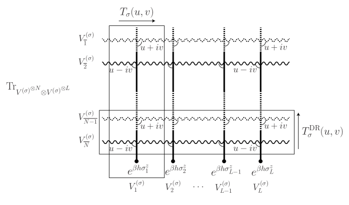
Figure 1: The QTM $T_{\sigma}(u,v)$ and the double-row transfer matrix $T^{\textrm{DR}}_{\sigma}(u,v)$ defined on the $N\times L$ square lattice, where $N\in 2\mathbb{N}_{+}$ is the Trotter number.

In the critical regime (2.42) restricted by the condition (2.43), the largest eigenvalue $\Lambda(u_{N},0)$ that gives the free energy of the model (see (3.8)) lies in the sector $M=N\sigma/2$. More explicitly, the BAE roots $\{\omega_{j}\}_{j=1}^{M}$ associated with the largest eigenvalue $\Lambda(u_{N},0)$ of the QTM $T_{\sigma}(u_{N},0)$ are given in the following form: $\{\omega_{j}\}=\{\omega_{l}^{k}\}$,

$$\omega_{l}^{k}\equiv\epsilon_{l}^{k}+i\delta_{l}^{k}+i(\sigma+1-2k)\ \ \textrm{mod}\ 2p_{0}i\quad(1\leq k\leq\sigma,\ 1\leq l\leq N/2).$$ (3.15)

Here, $\epsilon_{l}^{k}\in\mathbb{R}$ $(1\leq l\leq N/2)$ are symmetrically distributed about the imaginary axis for a given $k$, and $\delta_{l}^{k}\in\mathbb{R}$. In particular, in the high-temperature limit $\beta\to 0$ (i.e., $u_{N}\to 0$), we observe that the BAE roots (3.15) are reduced to $\omega_{l}^{k}=i(\sigma+1-2k)$. In fact, substituting them into (3.13) yields

$$\log\Lambda(u_{N}=0,v)=\log T_{\sigma}(u_{N}=0,v)=\log\left[\sum_{j=1}^{\sigma+1}\prod_{k=1}^{\sigma}\phi(v+2ik)\phi(v-2ik)\right],$$ (3.16)

and hence

$$\frac{\Lambda(u_{N}=0,0)}{\prod_{j=1}^{\sigma}b(2j)^{N}}=\sigma+1.$$ (3.17)

Thus, from (3.8), $-\lim_{\beta\to 0}\beta f$ (i.e, the entropy per site at $\beta=0$) reproduces the physically relevant result $-\lim_{\beta\to 0}\beta f=\log(\sigma+1)$.

3.2 TBA equation via $T$ and $Y$-functions

Our first goal is to relate the solutions to the TBA equations in terms of the $T$-functions (3.13). As shown in (3.8), the thermodynamic quantities of the spin-$\sigma/2$ XXZ chain are described by the largest eigenvalue of the QTM $T_{\sigma}(u_{N},v)$, which is given by (3.13) via the solutions to the BAE (3.14). However, in general, the Trotter limit $N\to\infty$ in (3.8) cannot be taken analytically by directly solving the BAE, except for the high-temperature limit $T=\infty$ (see (3.17)). To overcome this, we embed $T_{\sigma}(u_{N},v)$ into the functional relations ($T$ and $Y$-systems) that are fulfilled by the $T$-functions and their suitable combinations called $Y$-functions. By analyzing analytic properties, the $Y$-systems are mapped to the form of nonlinear integral equations, in which the Trotter limit can be taken analytically. These nonlinear integral equations are the TBA equations.

In what follows, the common variable $u$ in the $T$-functions is often omitted to simplify the notation. As previously described, the algebraic structure of $V^{(n)}$ of the QTM (3.7) is identical to that of the QTM for the spin-1/2 model. Consequently, the $T$-systems defined by (3.13) are the same as those obtained for the spin-1/2 model in [38]:

$$T_{n-1}(v+iy)T_{n-1}(v-iy)=T_{n+y-1}(v)T_{n-y-1}(v)+T_{y-1}(v+in)T_{y-1}(v-in),$$ (3.18)

which holds for any $v\in\mathbb{C}$, for any $\omega_{j}\in\mathbb{C}$ (referred to as the off-shell roots, implying that there is no requirement for $\omega_{j}$ to satisfy the BAE (3.14)), and for all integers $n,y\in\mathbb{N}_{+}$ such that $n\geq y\geq 1$. Note here that

$$T_{-1}(v)=0,\quad T_{0}(v)=\prod_{k=1}^{\sigma}\phi\left(v+i\left(u+\sigma-2\left(k-1\right)\right)\right)\phi\left(v-i\left(u-\sigma+2k\right)\right),$$ (3.19)

and the $T$-functions have the periodicity:

$$T_{n}(v+2p_{0}i)=T_{n}(v).$$ (3.20)

Now let us restrict ourselves to the case that $p_{0}$ defined in (2.42) (see also (2.43)) is a rational number and express it as the continued fraction form:

$$p_{0}=\left[\nu_{1},\nu_{2},\dots,\nu_{\alpha}\right]=\nu_{1}+\cfrac{1}{\nu_{2}+\cfrac{1}{\cfrac{\ddots}{\nu_{\alpha-1}+\cfrac{1}{\nu_{\alpha}}}}},$$ (3.21)

where $\alpha\geq 1$, $\nu_{2},\dots,\nu_{\alpha-1}\in\mathbb{N}_{+}$ and $\nu_{\alpha}\in\mathbb{N}_{\geq 2}$. We also set $\nu_{1}\in\mathbb{N}_{\geq 2}$ which comes from the condition $p_{0}\geq 2$ (see (2.42)). Note that irrational $p_{0}$ corresponds to $\alpha=\infty$. In Appendix A, we list the sequences required in this section: $\{m_{r}\}_{r=1}^{\alpha}$, $\{p_{r}\}_{r=1}^{\alpha}$, $\{y_{r}\}_{r=-1}^{\alpha}$, $\{z_{r}\}_{r=-1}^{\alpha}$, the TS-numbers $\{n_{j}\}_{j\geq 1}$ [27] defining the admissible lengths of the strings (2.45), and its slight modification $\{\widetilde{n}_{j}\}_{j\geq 1}$ [38]. We also introduce the sequence $\{w_{j}\}_{j\geq 1}$ and $\{\widetilde{w}_{j}\}_{j\geq 1}$ in (A.15). related to the string parity (A.17). All of these sequences are uniquely determined for a given value of $p_{0}$. In Appendix B, we prove that the restriction between the spin and the anisotropy, given by (2.43), is equivalent to the condition

$$\sigma+1\in\{\widetilde{n}_{j}\}_{j=1}^{m_{\alpha}}.$$ (3.22)

Hereafter, we consider the physical case where $\sigma$ and $p_{0}$ satisfies (3.22). Correspondingly, let us define the index $j_{\sigma}\in\{1,2,\dots,m_{\alpha}-1\}$ and $r_{\sigma}\in\{1,2,\dots,\alpha\}$ such that

$$\widetilde{n}_{j_{\sigma}+1}=\sigma+1,\quad m_{r_{\sigma}-1}<j_{\sigma}+1\leq m_{r_{\sigma}}\ (m_{r_{\sigma}-1}\leq j_{\sigma}<m_{r_{\sigma}}).$$ (3.23)

Note that $j_{\sigma=1}=1$ and $r_{\sigma=1}=1$ for any $p_{0}$ satisfying (3.21).

With the definitions provided above, we introduce a functional relation involving $T_{n}(v)$, as described in [38]:

$$T_{y_{\alpha}+y_{\alpha-1}-1}(v)=T_{y_{\alpha}-y_{\alpha-1}-1}(v)+2(-1)^{Mz_{\alpha}}\operatorname{ch}(y_{\alpha}\beta h)T_{y_{\alpha-1}-1}(v+iy_{\alpha}),$$ (3.24)

where $M$ denotes the number of BAE roots for (3.14). Note that this relation holds true for any off-shell roots, just as in equation (3.24). The proof can be straightforwardly completed using equation (A.8) and the following periodicities:

$$Q(v+2iy_{\alpha})=(-1)^{Mz_{\alpha}}Q(v),\quad\phi(v+2iy_{\alpha})=(-1)^{Nz_{\alpha}/2}\phi(v).$$ (3.25)

It is important to note that the relation (3.24) is valid only when $p_{0}$ is an arbitrary rational number as given by (3.21).

The $Y$-functions $\{Y_{j}(v)\}_{j=1}^{m_{\alpha}}$ are defined by the following combinations of the $T$-functions. For $m_{r}\leq j<m_{r+1}$ $(0\leq r\leq\alpha-1$) and $j\neq m_{\alpha}-1$,

$$Y_{j}(v):=\frac{T_{\widetilde{n}_{j+1}+y_{r}-1}\left(v+i(w_{j}+\widetilde{w}_{j_{\sigma}+1})p_{0}\right)T_{\widetilde{n}_{j+1}-y_{r}-1}\left(v+i(w_{j}+\widetilde{w}_{j_{\sigma}+1})p_{0}\right)}{T_{y_{r}-1}\left(v+i\widetilde{n}_{j+1}+i(w_{j}+\widetilde{w}_{j_{\sigma}+1})p_{0}\right)T_{y_{r}-1}\left(v-i\widetilde{n}_{j+1}+i(w_{j}+\widetilde{w}_{j_{\sigma}+1})p_{0}\right)},$$ (3.26)

while for $j=m_{\alpha}-1$ and $j=m_{\alpha}$,

$$Y_{m_{\alpha}-1}(v):=e^{y_{\alpha}\beta h}(-1)^{Mz_{\alpha}}\frac{T_{y_{\alpha}-y_{\alpha-1}-1}\left(v+i(w_{m_{\alpha}-1}+\widetilde{w}_{j_{\sigma}+1})p_{0}\right)}{T_{y_{\alpha-1}-1}\left(v+iy_{\alpha}+i(w_{m_{\alpha}-1}+\widetilde{w}_{j_{\sigma}+1})p_{0}\right)},$$

$$Y_{m_{\alpha}}(v)^{-1}:=e^{-y_{\alpha}\beta h}(-1)^{Mz_{\alpha}}\frac{T_{y_{\alpha}-y_{\alpha-1}-1}\left(v+i(w_{m_{\alpha}-1}+\widetilde{w}_{j_{\sigma}+1})p_{0}\right)}{T_{y_{\alpha-1}-1}\left(v+iy_{\alpha}+i(w_{m_{\alpha}-1}+\widetilde{w}_{j_{\sigma}+1})p_{0}\right)}.$$ (3.27)

We also set $Y_{0}(v):=0$ and $Y_{-1}(v)=\infty$. From the $T$-systems (3.18) and (3.24), we have

$$1+Y_{j}(v)=\frac{T_{\widetilde{n}_{j+1}-1}\left(v+iy_{r}+i(w_{j}+\widetilde{w}_{j_{\sigma}+1})p_{0}\right)T_{\widetilde{n}_{j+1}-1}\left(v-iy_{r}+i(w_{j}+\widetilde{w}_{j_{\sigma}+1})p_{0}\right)}{T_{y_{r}-1}\left(v+i\widetilde{n}_{j+1}+i(w_{j}+\widetilde{w}_{j_{\sigma}+1})p_{0}\right)T_{y_{r}-1}\left(v-i\widetilde{n}_{j+1}+i(w_{j}+\widetilde{w}_{j_{\sigma}+1})p_{0}\right)}$$ (3.28)

for $m_{r}\leq j<m_{r+1}$ $(0\leq r\leq\alpha-1$) and $j\neq m_{\alpha}-1$, and

$$\left(1+Y_{m_{\alpha}-1}(v)\right)\left(1+Y_{m_{\alpha}}(v)^{-1}\right)$$

$$\quad=\frac{T_{y_{\alpha}-1}\left(v+iy_{\alpha-1}+i(w_{m_{\alpha}-1}+\widetilde{w}_{j_{\sigma}+1})p_{0}\right)T_{y_{\alpha}-1}\left(v-iy_{\alpha-1}+i(w_{m_{\alpha}-1}+\widetilde{w}_{j_{\sigma}+1})p_{0}\right)}{T_{y_{\alpha-1}-1}\left(v+iy_{\alpha}+i(w_{m_{\alpha}-1}+\widetilde{w}_{j_{\sigma}+1})p_{0}\right)T_{y_{\alpha-1}-1}\left(v-iy_{\alpha}+i(w_{m_{\alpha}-1}+\widetilde{w}_{j_{\sigma}+1})p_{0}\right)}.$$ (3.29)

One finds that the above definitions of the $Y$-functions essentially the same with those introduced in [38] for the case where $h=0$ and $\sigma=1$. The sole distinction arises from a uniform shift in the argument that depends on $\sigma$, namely, $i\widetilde{w}_{j_{\sigma}+1}p_{0}$, which reflects the spin parity for the strings (2.45). Consequently, the $Y$-functions satisfy the same $Y$-systems as given by [38]:

$$\textrm{For }m_{r-1}\leq j\leq m_{r}-2\,\,(1\leq r\leq\alpha),$$

$$\quad Y_{j}(v+ip_{r})Y_{j}(v-ip_{r})=\left(1+Y_{j-1}(v)\right)^{1-2\delta_{j,m_{r-1}}}\left(1+Y_{j+1}(v)\right)\left(1+Y_{j+2}(v)^{-1}\right)^{\delta_{j,m_{\alpha}-2}},$$

$$\textrm{for }j=m_{r}-1\,\,(1\leq r\leq\alpha-1),$$

$$\quad Y_{j}(v+ip_{r}+ip_{r+1})Y_{j}(v+ip_{r}-ip_{r+1})Y_{j}(v-ip_{r}+ip_{r+1})Y_{j}(v-ip_{r}-ip_{r+1})$$

$$\qquad=\left[\left(1+Y_{j-1}(v+ip_{r+1})\right)\left(1+Y_{j-1}(v-ip_{r+1})\right)\right]^{1-2\delta_{j,m_{r-1}}}\left(1+Y_{j+1}(v+ip_{r})\right)$$

$$\qquad\quad\times\left(1+Y_{j+1}(v-ip_{r})\right)\left(1+Y_{j}(v+ip_{r}-ip_{r+1})\right)\left(1+Y_{j}(v-ip_{r}+ip_{r+1})\right),$$

$$\quad Y_{m_{\alpha}-1}(v+ip_{\alpha})Y_{m_{\alpha}-1}(v-ip_{\alpha})=e^{2y_{\alpha}\beta h}(1+Y_{m_{\alpha}-2}(v)),$$

$$\quad\left(Y_{m_{\alpha}}(v+ip_{\alpha})Y_{m_{\alpha}}(v-ip_{\alpha})\right)^{-1}=e^{-2y_{\alpha}\beta h}(1+Y_{m_{\alpha}-2}(v)),$$ (3.30)

which are valid for any off-shell roots. One can easily prove them by using (3.26), (3.27) and (3.28) in conjunction with property (3.20) and the definitions of the sequences $\{m_{r}\}$, $\{y_{r}\}$, $\{z_{r}\}$, $\{\widetilde{n}_{j}\}$ and $\{w_{j}\}$ given in Appendix A. By replacing $Y_{m_{\alpha-1}}(v)$ and $Y_{m_{\alpha}}(v)$ in (3.30) as

$$K(v):=e^{-y_{\alpha}\beta h}Y_{m_{\alpha-1}}(v)=e^{y_{\alpha}\beta h}Y_{m_{\alpha}}(v)^{-1},$$ (3.31)

the last two equalities in (3.30) reduce to

$$K(v+ip_{\alpha})K(v-ip_{\alpha})=1+Y_{m_{\alpha}-2}(v).$$ (3.32)

Then, by newly introducing

$$1+Y_{m_{\alpha-1}}(v):=(1+e^{y_{\alpha}\beta h}K(v))(1+e^{-y_{\alpha}\beta h}K(v))=K(v)^{2}+2\operatorname{ch}(y_{\alpha}\beta h)K(v)+1$$ (3.33)

in (3.30), we reproduce the $Y$-system originally introduced in [38]. In this paper, however, we use (3.30), because the physical structure of the quasi-particles, which is essential in the GHD formalism, is more clear.

By substituting a set of the BAE roots (on-shell roots) that gives the largest eigenvalue $\Lambda(u_{N},0)$ of the QTM $T_{\sigma}(u_{N},0)$, and examining the analytical properties of the $Y$-functions, the $Y$-systems are transformed into the following non-linear integral equations through the Fourier transform as explained in Appendix C.

In the non-linear integral equations (NLIEs), the Trotter limit $N\to\infty$ can be taken analytically. The resultant NLIEs read

For $$m_{r-1}\leq j\leq m_{r}-2\ (1\leq r\leq\alpha),$$

$$\log\eta_{j}(v)=\frac{2\pi\beta J\sin\theta}{\theta}(-1)^{r_{\sigma}}s_{r_{\sigma}}(v)\delta_{j,j_{\sigma}}+(1-2\delta_{j,m_{r-1}})s_{r}*\log(1+\eta_{j-1})(v)$$

$$\qquad\qquad\quad+s_{r}*\log(1+\eta_{j+1})(1+\eta_{j+2}^{-1})^{\delta_{j,m_{\alpha}-2}}(v),$$

for $$j=m_{r}-1\ (r_{\sigma}\leq r\leq\alpha-1),$$

$$\log\eta_{j}(v)=\frac{2\pi\beta J\sin\theta}{\theta}(-1)^{r_{\sigma}}s_{r_{\sigma}}(v)\delta_{j,j_{\sigma}}+(1-2\delta_{j,m_{r-1}})s_{r}*\log(1+\eta_{j-1})(v)$$

$$\qquad\qquad\quad+d_{r}*\log(1+\eta_{j})(v)+s_{r+1}*\log(1+\eta_{j+1})(v),$$

for $$j=m_{r}-1\ (1\leq r\leq r_{\sigma}-1),$$

$$\log\eta_{j}(v)=\frac{2\pi\beta J\sin\theta}{\theta}(-1)^{r}d_{r,\sigma}(v)+(1-2\delta_{j,m_{r-1}})s_{r}*\log(1+\eta_{j-1})(v)$$

$$\qquad\qquad\quad+d_{r}*\log(1+\eta_{j})(v)+s_{r+1}*\log(1+\eta_{j+1})(v),$$

$$\log\eta_{m_{\alpha}-1}(v)=y_{\alpha}\beta h+\frac{2\pi\beta J\sin\theta}{\theta}(-1)^{\alpha}s_{\alpha}(v)\delta_{j_{\sigma},m_{\alpha}-1}+s_{\alpha}*\log(1+\eta_{m_{\alpha}-2})(v),$$

$$\log\eta_{m_{\alpha}}(v)^{-1}=-y_{\alpha}\beta h+\frac{2\pi\beta J\sin\theta}{\theta}(-1)^{\alpha}s_{\alpha}(v)\delta_{j_{\sigma},m_{\alpha}-1}+s_{\alpha}*\log(1+\eta_{m_{\alpha}-2})(v),$$ (3.34)

where

$$\eta_{j}(v):=\lim_{N\to\infty}Y_{j}(v)\quad(1\leq j\leq m_{\alpha}),$$ (3.35)

and

$$s_{r}(v):=\frac{1}{4p_{r}\operatorname{ch}\left(\frac{\pi v}{2p_{r}}\right)},\quad d_{r}(v):=\int_{-\infty}^{\infty}e^{ikv}\frac{\operatorname{ch}(p_{r}-p_{r+1})k}{4\pi\operatorname{ch}(p_{r}k)\operatorname{ch}(p_{r+1}k)}dk,$$

$$d_{r,\sigma}(v):=\int_{-\infty}^{\infty}e^{ikv}\frac{\operatorname{ch}(\widetilde{q}_{j_{\sigma}+1}k)}{4\pi\operatorname{ch}(p_{r}k)\operatorname{ch}(p_{r+1}k)}dk=\int_{-\infty}^{\infty}e^{ikv}\frac{\operatorname{ch}\left(q_{j_{\sigma}}+(-1)^{r_{\sigma}}p_{r_{\sigma}}\right)k}{4\pi\operatorname{ch}(p_{r}k)\operatorname{ch}(p_{r+1}k)}dk,$$ (3.36)

with $\{q_{j}\}$ and $\{\widetilde{q}_{j}\}$ defined by (A.18).

We have numerically confirmed for wide ranges of $\sigma$ and $p_{0}$ that the solutions $\eta_{j}(v)$ to the above TBA equations agree with those obtained by the string hypothesis [33] as given in (2.49). The free energy (3.8) can be expressed in terms of $\eta_{j}(v)$ as (D.12). See Appendix D for detailed derivation of the free energy.

4 Drude weight

Now we evaluate the finite-temperature spin Drude weight at zero magnetic field (i.e., $h=0$). A general formula describing the Drude weight in terms of quantities determined by the generalized TBA equations (E.27) is explained in Appendix E, which is based on the arguments in [30, 7].

In general, the spin Drude weight is defined by the Kubo formula using the dynamical correlation functions in the equilibrium state:

$$D_{\textrm{s}}(\beta):=\beta\lim_{t\to\infty}\frac{1}{t}\int_{0}^{t}ds\int dx\langle j_{\textrm{s}}(s,x)j_{\textrm{s}}(0,0)\rangle^{\textrm{c}}=\beta\lim_{t\to\infty}\int dx\langle j_{\textrm{s}}(t,x)j_{\textrm{s}}(0,0)\rangle^{\textrm{c}},$$ (4.1)

where $j_{\textrm{s}}$ represents the spin current density, and $\langle\cdot\rangle^{\textrm{c}}$ denotes the thermal average of the connected correlation function: $\langle o_{1}o_{2}\rangle^{\textrm{c}}:=\langle o_{1}o_{2}\rangle-\langle o_{1}\rangle\langle o_{2}\rangle$ with $\langle\cdot\rangle$ defined as (2.33). Note that the quantity $D_{\textrm{s}}(\beta)/\beta$ is sometimes used as an alternative definition of the Drude weight. In such cases, the factor $\beta$ in front of the integral in (4.1) becomes unnecessary. However, in this paper, we adhere to the definition (4.1) as used in [14, 16]. For a generic expression of the Drude weight, see (E.1). The Drude weight $\mathsf{D}_{00}(\beta)$ in Appendix E is denoted as $D_{\textrm{s}}(\beta)$ in this section. By projecting the currents onto the space spanned by the local or quasi-local conserved charges, the dynamical current-current correlation function, defining the Drude weight, can be expressed in terms of equal-time current-charge and charge-charge correlation functions [30, 7] as given by (E.16).

For the present system (2.26), the local spin current $(j_{\textrm{s}})_{kk+1}$ ($1\leq k\leq L$) is determined by

$$(j_{\textrm{s}})_{kk+1}=i\left[(\mathcal{H}^{(\sigma)})_{kk+1},(q_{\textrm{s}})_{k+1}\right],\quad(q_{\textrm{s}})_{k}:=\frac{\sigma-\sigma_{k}^{z}}{2}$$ (4.2)

which follows from the discrete form of the continuity equation (cf. (E.2)):

$${\partial}_{t}(q_{\textrm{s}})_{k}+\left[(j_{\textrm{s}})_{kk+1}-(j_{\textrm{s}})_{kk+1}\right]=0,$$ (4.3)

where ${\partial}_{t}(q_{\textrm{s}})_{k}=i\left[\mathcal{H}^{(\sigma)},(q_{\textrm{s}})_{k}\right]$. The corresponding quantities $(\widetilde{q}_{\textrm{s}})_{k}$ and $(\widetilde{j}_{\textrm{s}})_{k}$ (see (2.32)) are also given by

$$(\widetilde{q}_{\textrm{s}})_{k}=F^{(\sigma)}\left[(q_{\textrm{s}})_{k}\right]{F^{(\sigma)}}^{-1}=(q_{\textrm{s}})_{k},$$

$$(\widetilde{j}_{\textrm{s}})_{kk+1}=F^{(\sigma)}\left[(j_{\textrm{s}})_{kk+1}\right]{F^{(\sigma)}}^{-1}=i\left[(\widetilde{\mathcal{H}}^{(\sigma)})_{kk+1},(\widetilde{q}_{\textrm{s}})_{k+1}\right]=i\left[(\widetilde{\mathcal{H}}^{(\sigma)})_{kk+1},(q_{\textrm{s}})_{k+1}\right],$$ (4.4)

where the second equality in the first equation is due to the fact that $F^{(\sigma)}$ and $\sigma_{k}^{z}$ are diagonal matrices.

The averages of (4.2) over the GGE (see (E.6)) can be expressed in terms of a mode decomposition using the $n_{j}$-string ($1\leq j\leq m_{\alpha}$) as shown in (E.17), (E.32), and (E.33). They reduce to

$$\left\langle(q_{\textrm{s}})_{k}\right\rangle=\left\langle(\widetilde{q}_{\textrm{s}})_{k}\right\rangle=\sum_{j=1}^{m_{\alpha}}\int_{-\infty}^{\infty}dv\,\rho_{j}(v)h_{\textrm{s};j}(v),$$

$$\left\langle(j_{\textrm{s}})_{kk+1}\right\rangle=\left\langle(\widetilde{j}_{\textrm{s}})_{kk+1}\right\rangle=\sum_{j=1}^{m_{\alpha}}\int_{-\infty}^{\infty}dv\,\rho_{j}(v)v_{j}^{\textrm{eff}}(v)h_{\textrm{s};j}(v),$$ (4.5)

where

$$\left\langle(j_{\textrm{s}})_{kk+1}\right\rangle=\left\langle(\widetilde{j}_{\textrm{s}})_{kk+1}\right\rangle=0$$ (4.6)

must hold, since $\langle\cdot\rangle$ and $\langle\widetilde{\cdot}\rangle$ defined as (2.33) denote the equilibrium thermal average (cf. (E.6)). In (4.5), the first equalities are derived from (2.34), $\rho_{j}(v)$ is the distribution function associated with the $n_{j}$-string, and $h_{\textrm{s};j}(v)$ (corresponding to $h_{0;j}(v)$ in Appendix E) denotes the bare spin, which is the number of magnons composing the $n_{j}$-string, i.e., $h_{\textrm{s};j}(v)=h_{0;j}(v)=n_{j}$. Accordingly, by (2.49) and (E.27), we identify

$$\beta^{0}=2\beta h$$ (4.7)

in the present case. The effective velocity, $v_{j}^{\textrm{eff}}(v)$, is generally described by (E.31) via the generalized TBA equations (E.27). In the context of our present case, it is defined as

$$v_{j}^{\textrm{eff}}(v)=\frac{\beta^{-1}{\partial}_{v}\log\eta_{j}(v)}{\epsilon{\partial}_{\beta}\log\eta_{j}(v)},\quad\epsilon=-\frac{\theta}{J\sin\theta},$$ (4.8)

where $\eta_{j}(v)$ is determined by the standard TBA equations (3.34), which are equivalent to (2.49). As $v_{j}^{\text{eff}}(v)$ in (4.8) is an odd function while $\rho_{j}(v)$ and $h_{\textrm{s};j}(v)$ are even functions, we can easily confirm (4.6). Then, using the procedure described in [30, 7], which is also summarized in Appendix E, we can express the spin Drude weight as

$$D_{\textrm{s}}(\beta)=\beta\sum_{j=1}^{m_{\alpha}}\int dv\,\rho_{j}(v)\left(1-\vartheta_{j}(v)\right)\left[v^{\textrm{eff}}_{j}(v)h_{0;j}^{\textrm{dr}}(v)\right]^{2}.$$ (4.9)

Here, $h_{0;j}^{\textrm{dr}}(v)$ represents the dressed spin, which is defined as

$$h_{0;j}^{\textrm{dr}}(v)={\partial}_{\beta^{0}}\log\eta_{j}(v)={\partial}_{2\beta h}\log\eta_{j}(v),$$ (4.10)

as indicated in (4.7) and (E.29). Moreover, according to the TBA equations (3.34), for zero magnetic field ($h=0$), the value of $h_{0;j}^{\textrm{dr}}(v)$ is

$$h_{0;j}^{\textrm{dr}}(v)=\begin{dcases}\frac{y_{\alpha}}{2}&\text{if $j=m_{\alpha},m_{\alpha-1}$}\\ 0&\text{otherwise}\end{dcases}.$$ (4.11)

Inserting $\eta_{j}(v):=\rho^{\textrm{h}}_{j}(v)/\rho_{j}(v)$, where $\rho^{\textrm{h}}_{j}(v)$ is the hole density of the $n_{j}$-string, into the fermionic distribution function $\vartheta_{j}(v)$ (eq. (E.20)) with the density of states $\rho^{\textrm{tot}}_{j}(v):=\rho_{j}(v)+\rho^{\textrm{h}}_{j}(v)$, we obtain

$$\rho_{j}(v)(1-\vartheta_{j}(v))=\frac{\rho^{\textrm{tot}}_{j}(v)}{(1+\eta_{j}(v))(1+\eta^{-1}_{j}(v))}=\frac{\epsilon\xi_{j}{\partial}_{\beta}\log\eta_{j}(v)}{2\pi(1+\eta_{j}(v))(1+\eta^{-1}_{j}(v))}.$$ (4.12)

Here $\xi_{j}$ is a sign factor defined in (2.48). To derive the last equality, we have used (E.30) with $\varepsilon_{j}^{\textrm{dr}}(v)={\partial}_{\beta^{1}}\log\eta_{j}(v)={\partial}_{\beta}\log\eta_{j}(v)$ which follows from (E.29), (E.18) and (E.19). By substituting (4.8), (4.11) and (4.12) into (4.9), and taking into account

$$\xi_{m_{\alpha}}=\operatorname{sgn}(q_{m_{\alpha}})=-\xi_{m_{\alpha}-1}=(-1)^{\alpha}$$ (4.13)

along with the identity $\eta_{m_{\alpha}}(v)^{-1}=\eta_{m_{\alpha}-1}(v)$ which holds for $h=0$, one sees that only the last two $\eta$-functions $\eta_{\alpha-1}$ and $\eta_{\alpha}$ contribute to the Drude weight at $h=0$. Explicitly it reads

$$D_{\textrm{s}}(\beta)=(-1)^{\alpha}\frac{\beta y_{\alpha}^{2}J\sin\theta}{4\pi\theta}\int_{-\infty}^{\infty}\frac{\left(\beta^{-1}{\partial}_{v}\log\eta_{m_{\alpha}-1}(v)\right)^{2}}{\left(1+\eta_{m_{\alpha}-1}(v)\right)\left(1+\eta_{m_{\alpha}-1}^{-1}(v)\right){\partial}_{\beta}\log\eta_{m_{\alpha}-1}(v)}dv.$$ (4.14)

The formula presented above (4.14) is formally the same as that for the spin-1/2 model [14, 65, 16, 17]. The spin dependency is given through the $\eta$-functions (3.34).

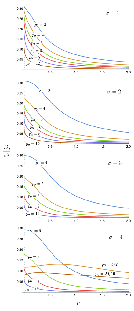
Figure 2: Temperature-dependence of the spin Drude weight (divided by $\sigma^{2}$) $D_{\textrm{s}}/\sigma^{2}$ for $J=1$, $S=\sigma/2$ ($\sigma=1,2,3,4$) and various anisotropies $\Delta=\cos(\pi/p_{0})$. $D_{\textrm{s}}/\sigma^{2}$ smoothly varies with respect to $T$ and approaches zero at the isotropic limit $p_{0}\to\infty$ ($\Delta\to 1$). For $\sigma=4$, the admissible region of $p_{0}$ is separated into two intervals: $p_{0}\in(2,3)$ and $p_{0}\in(4,\infty)$ as in Table 1. The behavior of $D_{\textrm{s}}/\sigma^{2}$ in each region distinctly differs, reflecting the fact that the structure of the energy spectrum characterized by the strings is essentially different in each interval.

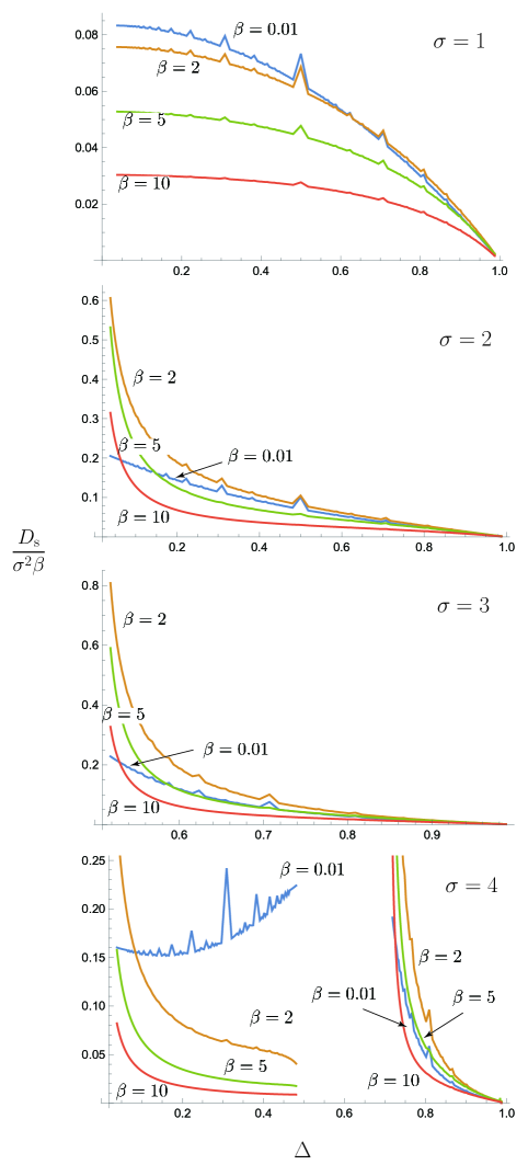
Figure 3: Popcorn structure of the Drude weight (divided by temperature $\beta=1/T$ and $\sigma^{2}$) $D_{\textrm{s}}/(\sigma^{2}\beta)$ for $J=1$, $S=\sigma/2$ ($\sigma=1,2,3,4$). $D_{\textrm{s}}/(\sigma^{2}\beta)$ exhibits discontinuities throughout the anisotropy $\Delta=\cos(\pi/p_{0})$. The physically admissible region for $\Delta$ depends on $S$. Refer to (2.43) and Table 1 for details.

We solved the TBA equations numerically to compute the spin Drude weight (4.14). In Fig. 2, the temperature-dependence of the Drude weight (divided by $\sigma^{2}$) $D_{\textrm{s}}(\beta)/\sigma^{2}$ is shown for the cases where the model with $\sigma=1,2,3,4$ ($S=\sigma/2$) in the antiferromagnetic regime $J=1$. Although the dependencies for $\sigma=1$ have already been known in [14, 16], we included them for the sake of comparison. As mentioned earlier, the physically admissible region of $\Delta$ is restricted as in (2.43) (refer to Table 1 for concrete examples). For a given $\Delta$ and $\sigma$, the Drude weight varies smoothly with the temperature, and approaches zero at the isotropic limit $p_{0}\to\infty$ ($\Delta\to 1$). Notably, when the admissible region of $\Delta$ consists of separate intervals (as with $\sigma=4$ in the figure, where the admissible region of $p_{0}$ is separated into two intervals: $p_{0}\in(2,3)$ and $p_{0}\in(4,\infty)$), the behavior of the Drude weight differs distinctly in each region. As pointed out in [33, 50, 36, 37], the ground state and the low-lying excitations in each region are characterized by different types of strings. Accordingly, the low-energy properties in each region are described by a different conformal field theory [37]. The different behavior of the Drude weight can be interpreted by these differences in the structure of the energy spectrum.

In Fig. 3, we also depict the anisotropy dependence of the Drude weight for $J=1$ divided by $\beta=1/T$ and $\sigma^{2}$, i.e., $D_{\rm s}/(\beta^{2}\sigma^{2})$. Again, for comparison, we include the known results [16] for $\sigma=1$. For a given $T$ and $\sigma$, the anisotropy dependence of the Drude weight exhibits the characteristic popcorn structure. The popcorn structure is suppressed with the decrease in temperature and will eventually exhibit a smooth curve depending on $\Delta$ at the zero-temperature limit.

5 High-temperature limit

We aim to derive an analytical expression for the high-temperature behavior of the Drude weight at $h=0$ (4.14), namely $\lim_{\beta\to 0}D_{\textrm{s}}(\beta)/\beta$. Given the complexity of the TBA equations, we take a different approach by adopting and extending the method developed in [16] for the spin-1/2 case. Namely, we evaluate this limit by directly examining the high-temperature behavior of the $T$ and $Y$-functions, as defined in equations (3.13), (3.26) and (3.27).

In fact, according to the definition of free energy given by equations (3.6) through (3.4) and (3.5), considering only the case $N=2$ would suffice for evaluating contributions of $O(\beta)$. However, in this work, we extend the discussion to arbitrary even values of $N$ to make the argument more generally applicable. The behavior of $T_{n}(u_{N},v)$ at $O(\beta)$ can be evaluated by inserting the BAE roots, specifically those given by (3.15), up to terms of $O(\beta)$. Since the real parts of the roots are symmetrically distributed with respect to the imaginary axis, we have $\sum_{l=1}^{N/2}\epsilon_{l}^{k}=0$ for $1\leq k\leq\sigma$. Therefore, the $O(\beta)$ contributions from $\epsilon_{l}^{k}$ to $T(u_{N},v)$ cancel each other out. Conversely, the contributions from $\delta_{l}^{k}$ are retained in the form of the total sum $\delta^{k}:=\sum_{l=1}^{N/2}\delta_{l}^{k}$.

The quantity $\delta^{k}$ is obtained as follows. First, substituting $u=u_{N}$ and (3.15) into (3.14), and using the fact that $z_{l}^{k}:=\epsilon_{l}^{k}+i\delta_{l}^{k}$ and $u_{N}$ are both $O(\beta)$, we obtain

$$P_{k}(z_{l}^{k})=0\quad(1\leq k\leq\sigma,\ 1\leq l\leq N/2),$$ (5.1)

where

$$P_{k}(z):=\prod_{l=1}^{N/2}(z-z_{l}^{k-1})+\prod_{l=1}^{N/2}(z-z_{l}^{k+1}),$$ (5.2)

and $z_{l}^{0}:=-iu_{N}$ and $z_{l}^{\sigma+1}:=iu_{N}$ ($1\leq l\leq N/2$). Second, due to (5.1), we can rewrite $P_{k}(z)$ as $P_{k}(z)=2\prod_{l=1}^{N/2}(z-z_{l}^{k})$, where the overall constant has been determined by the leading coefficient of $z^{N/2}$ in (5.2). Then, by comparing the coefficients of $z^{N/2-1}$, we obtain $2\sum_{l}z_{l}^{k}=\sum_{l}(z_{l}^{k-1}+z_{l}^{k+1})$, which leads to $\delta^{k}=(\delta^{k-1}+\delta^{k+1})/2$. Here we have used the equality $\sum_{l=1}^{N/2}\epsilon^{k}_{l}=0$. Finally, imposing the condition $\delta^{1}=-\delta^{\sigma}$, which comes from the symmetrical argument, we arrive at

$$\delta^{k}:=\sum_{l=1}^{N/2}\delta_{l}^{k}=-\frac{Nu_{N}}{2}\left(1-\frac{2k}{\sigma+1}\right)=\frac{J\sin\theta}{2\theta}\left(1-\frac{2k}{\sigma+1}\right)\beta.$$ (5.3)

By inserting this equation into (3.13), we can explicitly calculate the $O(\beta)$ behavior of $\eta_{j}(v)$ ($1\leq j\leq m_{\alpha}$) via the formula (3.26), (3.27) and (3.35), and consequently, also determine the $O(\beta)$ behavior of the Drude weight (4.14).

According to (4.14), only the function $Y_{m_{\alpha-1}}(v)$ needs to be considered for the Drude weight at $h=0$. Combining (3.27) and (3.24) at $h=0$, we obtain

$$1+Y_{m_{\alpha}-1}(v)=\frac{(-1)^{Mz_{\alpha}}T_{y_{\alpha}+y_{\alpha-1}-1}(v^{\prime})-T_{y_{\alpha-1}-1}(v^{\prime}+iy_{\alpha})}{T_{y_{\alpha-1}-1}(v^{\prime}+iy_{\alpha})},$$ (5.4)

where we introduce

$$v^{\prime}:=v+i(w_{m_{\alpha}-1}+\widetilde{w}_{j_{\sigma}+1})p_{0},$$ (5.5)

to simplify subsequent notations. Inserting equation (3.13), decomposing the summation appearing in $T_{y_{\alpha}+y_{\alpha-1}-1}(v^{\prime})$ into two parts as $\sum_{j=1}^{y_{\alpha}+y_{\alpha-1}}=\sum_{j=1}^{y_{\alpha-1}}+\sum_{j=y_{\alpha-1}+1}^{y_{\alpha}+y_{\alpha-1}}$, and using the periodicities (3.25), one obtains

$$1+Y_{m_{\alpha}-1}(v)=\frac{f(v)}{g(v)},$$

$$f(v):=\frac{T_{y_{\alpha}-1}(v^{\prime}+iy_{\alpha-1})}{Q\left(v^{\prime}+i(y_{\alpha}+y_{\alpha-1})\right)Q\left(v^{\prime}-i(y_{\alpha}-y_{\alpha-1})\right)},$$

$$g(v):=\frac{T_{y_{\alpha-1}-1}(v^{\prime}+iy_{\alpha})}{Q\left(v^{\prime}+i(y_{\alpha}+y_{\alpha-1})\right)Q\left(v^{\prime}+i(y_{\alpha}-y_{\alpha-1})\right)}.$$ (5.6)

Due to the BAE (3.14) and periodicities given in (3.25), $f(v)$ is an entire function and is bounded. Therefore, by Liouville’s theorem, $f(v)$ must be a constant which is calculated by taking the limit $v\to\infty$. Using $\sum_{j=1}^{M}\omega_{j}=0$, it explicitly reads

$$f(v)=\frac{y_{\alpha}}{(\sin\theta)^{2M}}.$$ (5.7)

Taking into account (3.5) and (5.3), and expanding $g(v)$ up to $O(\beta)$, we obtain

$$1+\eta_{m_{\alpha}-1}(v)=\lim_{N\to\infty}(1+Y_{m_{\alpha}-1}(v))$$

$$\qquad=\frac{y_{\alpha}}{y_{\alpha-1}}\Bigg{\{}1-i\frac{\beta J\sin\theta}{2y_{\alpha-1}}\sum_{k=1}^{\sigma}k\left(1-\frac{k}{\sigma+1}\right)\left[\coth\frac{\theta}{2}\left(v^{\prime}-i(y_{\alpha}+y_{\alpha-1}+\sigma+1-2k)\right)\right.$$

$$\qquad\qquad\qquad\quad\left.-\coth\frac{\theta}{2}\left(v^{\prime}-i(y_{\alpha}-y_{\alpha-1}+\sigma+1-2k)\right)\right]\Biggr{\}}+O(\beta^{2}).$$ (5.8)

Substituting (5.5) in the above and using

$$y_{\alpha}\pm y_{\alpha-1}+w_{m_{\alpha-1}}p_{0}\equiv\pm(-1)^{\alpha-1}p_{\alpha}+p_{0}\ \ \textrm{mod}\ 2p_{0}$$ (5.9)

lead to

$$1+\eta_{m_{\alpha}-1}(v)$$

$$\ =\frac{y_{\alpha}}{y_{\alpha-1}}\left[1-\frac{2\pi\beta J\sin\theta}{\theta y_{\alpha-1}}\sum_{k=1}^{\sigma}k\left(1-\frac{k}{\sigma+1}\right)a_{m_{\alpha}-1}\left(v-i(\sigma+1-2k+\widetilde{w}_{j_{\sigma}+1}p_{0})\right)\right]+O(\beta^{2}),$$ (5.10)

where the function $a_{j}(v)$ is defined as

$$a_{j}(v):=\frac{\theta}{2\pi}\frac{\sin(\theta q_{j})}{\operatorname{ch}(\theta v)+\cos(\theta q_{j})}.$$ (5.11)

Finally, the insertion of (5.10) into (4.14) yields

$$\lim_{\beta\to 0}\beta^{-1}D_{\textrm{s}}(\beta) =\frac{(-1)^{\alpha+1}y_{\alpha}}{2}\left(\frac{J\sin\theta}{\theta}\right)^{2}$$

$$\ \times\int_{-\infty}^{\infty}\frac{\left[\sum_{k=1}^{\sigma}k\left(1-\frac{k}{\sigma+1}\right)a^{\prime}_{m_{\alpha}-1}\left(v-i(\sigma+1-2k+\widetilde{w}_{j_{\sigma}+1}p_{0})\right)\right]^{2}}{\sum_{k=1}^{\sigma}k\left(1-\frac{k}{\sigma+1}\right)a_{m_{\alpha}-1}\left(v-i(\sigma+1-2k+\widetilde{w}_{j_{\sigma}+1}p_{0})\right)}dv.$$ (5.12)

For $S=1/2$ ($\sigma=1$), (5.12) coincides with the result obtained in [16] up to an overall factor, which is due to the difference in the definition of the coupling constant $J$. In this case, the integral can be explicitly computed in [16], yielding:

$$\left.\lim_{{\beta\to 0}}D_{\textrm{s}}(\beta)\right|_{\sigma=1}=\frac{(J\sin\theta)^{2}}{8\sin^{2}\frac{\pi}{y_{\alpha}}}\left(1-\frac{y_{\alpha}}{2\pi}\sin\frac{2\pi}{y_{\alpha}}\right).$$ (5.13)

This result is consistent with the Prosen-Ilievski bound [15] derived via the construction of quasi-local conserved charges [66, 67]. On the other hand, for spins higher than $1/2$, the integrand becomes more complicated. It appears difficult to calculate it explicitly when $p_{0}$ is a generic rational number. For $S=1$ ($\sigma=2$), the integral can be explicitly calculated for $\alpha=1$, i.e., $p_{0}=\pi/\nu_{1}$. The result is

$$\left.\lim_{{\beta\to 0}}D_{\textrm{s}}(\beta)\right|_{\sigma=2,\alpha=1}=\frac{J^{2}}{12\cos^{2}\frac{\pi}{\nu_{1}}}\left(1-\frac{\nu_{1}}{4\pi}\sin\frac{4\pi}{\nu_{1}}\right),$$ (5.14)

which exactly coincides with the result recently derived in [28].

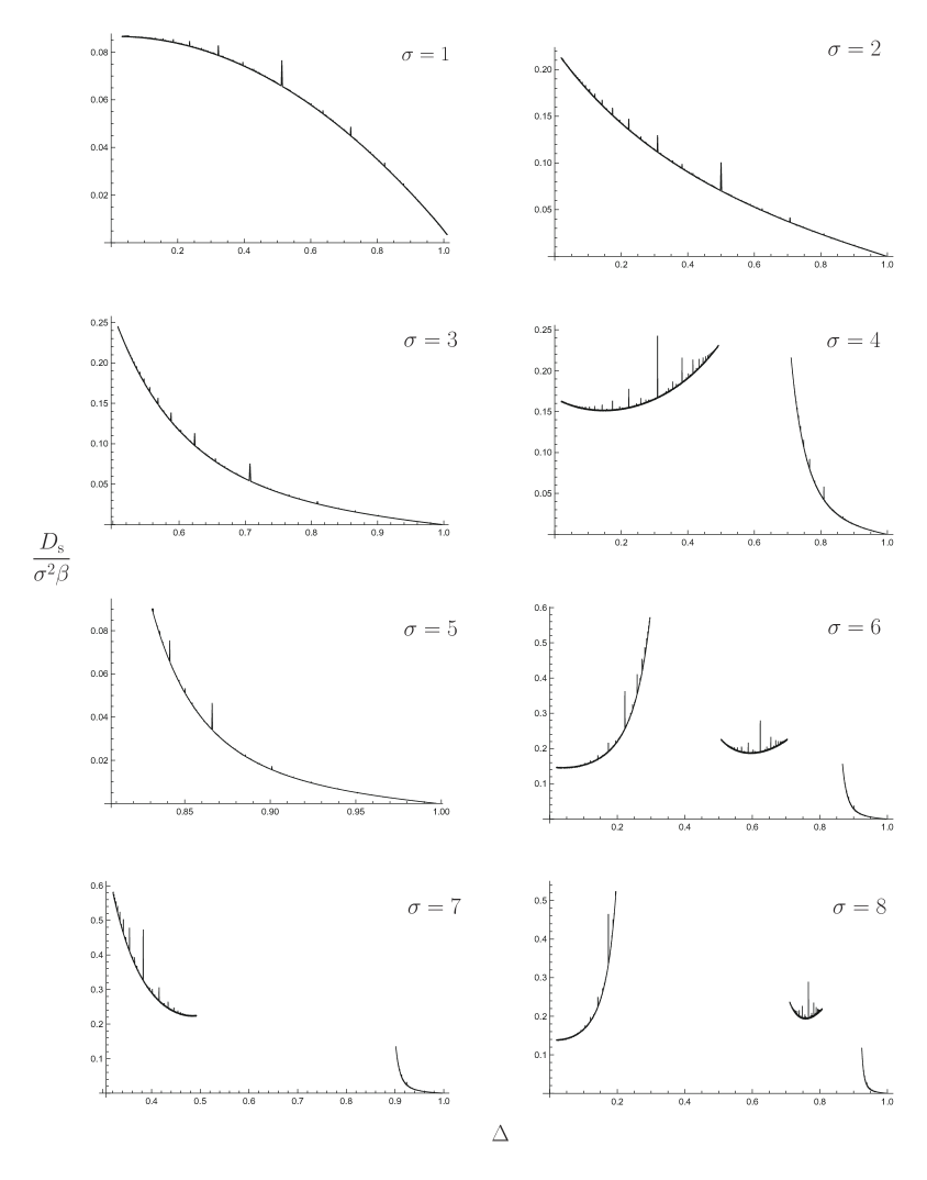
Figure 4: High-temperature limit of the spin Drude weight (divided by $\beta=1/T$) with $J=\pm 1$ and $S=\sigma/2$ ($1\leq\sigma\leq 8$) for the anisotropy dependence. The graph displays popcorn structures, indicating everywhere discontinuity with respect to $\Delta$. For the physically admissible region of $\Delta$, refer to Eq. (2.43) and Table 1.

In Fig. 4, we depict the high-temperature limit $\beta\to 0$ of $D_{\textrm{s}}(\beta)/(\sigma^{2}\beta)$. The result for $\sigma=1$ is referred to as the Prosen-Ilievski bound [15]. For $\sigma\geq 2$, the spin Drude weights exhibit a prominent popcorn structure similar to the $\sigma=1$ case. For $p_{0}$ close to, but not exactly on, the irrational value, which can be obtained with the desired precision by taking the limit $\alpha\to\infty$, the Drude weights are approximately represented by the points on the curve. Namely, the Drude weight behaves like a continuous function for $p_{0}$ close to the irrational value, but is discontinuous everywhere for rational $p_{0}$. The Drude weight cannot be obtained in the present approach when $p_{0}$ is exactly an irrational number.

6 Summary and Discussion

We have examined the finite-temperature spin Drude weight for the integrable XXZ chain with arbitrary spin $S$ at zero magnetic field. In the critical regime, the admissible string lengths are described by the TS-numbers, akin to the spin-1/2 case. In relation to this, the Drude weight exhibits a behavior similar to that observed in the spin-1/2 XXZ, displaying a pronounced popcorn structure that is discontinuous everywhere with respect to the anisotropy parameter $\Delta$. For a given $S$, the admissible region of $\Delta$, in general, comprises several separate intervals, which is a fundamental distinction from the spin-1/2 case. Importantly, the structure of the TBA equations in each region is distinct, resulting in the Drude weight behaving drastically differently in each region. In this work, we have constructed the TBA equations, using the QTMs and their functional relations. As a significant advantage, this approach enables us to perform a systematic exact calculation of the spin Drude weight in the high-temperature limit.

Let us briefly discuss the open problems that remain unresolved in this work. First, the low-temperature behavior, including the zero-temperature limit of the Drude weight, has not yet been calculated. In contrast, for the spin-1/2 case, the low-temperature behavior of the Drude weight has been recently addressed and calculated [68]. While the low-temperature properties of the present model are more intricate than those of the spin-1/2 case, the procedure used there might be useful to our current model.

Second, the investigation of spin diffusion at the isotropic point $\Delta=1$ is crucial. At this point, along with the massive region $\Delta>1$, the spin Drude weight vanishes, suggesting diffusive spin transport [19, 69, 70]. In fact, behavior similar to the divergence observed in the spin-1/2 case of the diffusion constant has also been noted in higher spin cases [19], indicating superdiffusive behavior. There is considerable interest in examining this property through more quantitative approaches, such as deriving a rigorous dynamical exponent.

Third, the Drude weight cannot be derived in our current procedure when $p_{0}$ is exactly on irrational numbers. Of course, as described before, taking the limit $\alpha\to\infty$, we may obtain the Drude weight when $p_{0}$ is in arbitrary vicinity of an irrational number. Indeed, the expression at infinite temperature (see (5.12)) indicates that the Drude weight converges to a certain finite value in this limit. However, it remains unclear whether this convergence value actually corresponds to the real Drude weight on $p_{0}$ when it is irrational.

Fourth, the spin Drude weight may also be evaluated using Kohn’s formula [26]. Namely, by imposing a twisted boundary condition on the row transfer matrix (2.20), achieved through the multiplication of the factor $\exp\left[-i\phi(n-\sigma_{\overline{1}}^{z})/2\right]$ inside the trace, where $\sigma_{\overline{1}}^{z}$ is the $z$-component of the spin-$n/2$ operator acting on $V_{\overline{1}}^{(n)}$, the Drude weight is determined by the expectation value of the curvature of the energy spectrum with respect to the twist angle $\phi$:

$$D_{\textrm{s}}(\beta)=\lim_{L\to\infty}\frac{1}{L}\sum_{n}\left.\frac{d^{2}E_{n}(\phi)}{d\phi^{2}}\right|_{\phi=0}e^{-\beta E_{n}(0)}.$$ (6.1)

In the above, $E_{n}(\phi)$ denotes the $n$th eigenvalue of the operator obtained by taking the logarithmic derivative of the twisted row transfer matrix. Note that the integrable structure (2.21) is preserved even under the twisted boundary condition. Note that the integrable structure (2.21) is preserved even under the twisted boundary condition. Furthermore, the Hamiltonian is obtained by the same similarity transformation as in (2.26), with eigenvalues that are formally in the same form as (2.41). The effect of the twisted boundary condition is incorporated into the BAE (2.40) by multiplying the RHS with the factor $e^{-i\phi}$, leading to a shift in the string center in (2.45) from $\lambda_{\mu}^{n_{j}}$ to $\lambda_{\mu}^{n_{j}}(\phi)$. By expanding $E_{n}(\phi)$ up to second order in $\phi$ and explicitly evaluating (6.1), in a manner similar to Zotos’s approach for the $\sigma=1$ case, it might be possible to reproduce the formula given by (4.14).

Finally, utilizing the QTMs developed in this study, we can systematically calculate the infinite temperature Onsager matrix element associated with spin transport for the $S=1/2$ chain in a zero magnetic field. This becomes feasible because the dressed scattering kernel for the $S=1/2$ model at infinite temperature can be determined using the TBA equations for an $S>1/2$ model. Our detailed analysis uncovers an intriguing popcorn structure of the Onsager matrix element. Further details will be reported in an upcoming publication (see [71]).

Appendix A Takahashi-Suzuki (TS) numbers

Given anisotropy $\theta$, it is known that the admissible lengths of string solutions of the Bethe ansatz equation (2.40) are given by the so-called Takahashi-Suzuki (TS) numbers generated by the continued fraction expansion of $p_{0}:=\pi/\theta$ (eq. (3.21)). Here, we summarize the TS-numbers [27, 38] and related sequences required for the formulation.

Given $\{\nu_{r}\}_{r=1}^{\alpha}$ in (3.21), we define the sequences $\{m_{r}\}_{r=0}^{\alpha+1}$ and $\{p_{r}\}_{r=0}^{\alpha+1}$ by

$$m_{r}=\nu_{1}+\nu_{2}+\cdots+\nu_{r}\quad(0\leq r\leq\alpha),\quad m_{\alpha+1}=\infty,$$ (A.1)

and

$$p_{0}=\frac{\pi}{\theta}=[\nu_{1},\dots,\nu_{\alpha}],\quad p_{1}=1,\quad p_{r}=p_{r-2}-\nu_{r-1}p_{r-1}\quad(2\leq r\leq\alpha+1),$$ (A.2)

respectively. More explicitly, $p_{r}$ ($r\geq 1$) reads

$$p_{r}=\prod_{s=2}^{r}\frac{1}{[\nu_{s},\dots,\nu_{\alpha}]}\ \ \text{for $1\leq r\leq\alpha$}.$$ (A.3)

From this expression and (A.2), one easily finds that

$$p_{\alpha+1}=0,\quad[\nu_{r},\dots,\nu_{\alpha}]=\frac{p_{r-1}}{p_{r}},\quad\nu_{r}=\left\lfloor\frac{p_{r-1}}{p_{r}}\right\rfloor.$$ (A.4)

Define the sequences $\{y_{r}\}_{r=-1}^{\alpha}$ and $\{z_{r}\}_{r=-1}^{\alpha}$ by

$$y_{-1}=0, \quad y_{0}=1, \quad y_{r}=y_{r-2}+\nu_{r}y_{r-1}\ \ (1\leq r\leq\alpha),$$

$$z_{-1}=1, \quad z_{0}=0, \quad z_{r}=z_{r-2}+\nu_{r}z_{r-1}\ \ (1\leq r\leq\alpha).$$ (A.5)

Then by induction, one sees that

$$[\nu_{1},\dots,\nu_{r}]=\frac{y_{r}}{z_{r}}\quad(1\leq r\leq\alpha),\quad y_{r}=p_{0}z_{r}+(-1)^{r}p_{r+1}\quad(-1\leq r\leq\alpha),$$ (A.6)

where we extend integers $\nu_{r}$ $(1\leq r\leq\alpha)$ formally to real numbers and use

$$[\nu_{1},\dots,\nu_{r},\nu_{r+1}]=\left[\nu_{1},\dots,\nu_{r-1},\nu_{r}+\frac{1}{\nu_{r+1}}\right]$$ (A.7)

to prove the first equality. In particular,

$$p_{0}=\frac{y_{\alpha}}{z_{\alpha}}.$$ (A.8)

Let $y_{r}=:f_{r}(\nu_{1},\dots,\nu_{r})$. From (A.5), the equality $z_{r+1}=f_{r}(\nu_{2},\dots,\nu_{r+1})$ holds. Also, one finds that

$$f_{r}(\nu_{1},\dots,\nu_{r})=f_{r}(\nu_{r},\dots,\nu_{1}),$$ (A.9)

which can be shown by induction. Indeed, one directly sees that it holds for $1\leq r\leq 4$. Assume that the equality also holds for $r=s-k$ ($s\geq 5$; $1\leq k\leq 4$). Then, using (A.5) and the assumptions, one obtains

$$f_{s}(\nu_{1},\dots,\nu_{s}) =\nu_{s}f_{s-1}(\nu_{1},\dots,\nu_{s-1})+f_{s-2}(\nu_{1},\dots,\nu_{s-2})$$

$$=\nu_{s}f_{s-1}(\nu_{s-1},\dots,\nu_{1})+f_{s-2}(\nu_{s-2},\dots,\nu_{1})$$

$$=\nu_{s}\left[\nu_{1}f_{s-2}(\nu_{s-1},\dots,\nu_{2})+f_{s-3}(\nu_{s-1},\dots,\nu_{3})\right]$$

$$\qquad+\nu_{1}f_{s-3}(\nu_{s-2},\dots,\nu_{2})+f_{s-4}(\nu_{s-2},\dots,\nu_{3})$$

$$=\nu_{1}f_{s-1}(\nu_{s},\dots,\nu_{2})+f_{s-2}(\nu_{s},\dots,\nu_{3})$$

$$=f_{s}(\nu_{s},\dots,\nu_{1}).$$ (A.10)

Thus, (A.9) holds. (A.5) yields

$$f_{r}(\nu_{r},\dots,\nu_{1})=\nu_{1}f_{r-1}(\nu_{r},\dots,\nu_{2})+f_{r-2}(\nu_{r},\dots,\nu_{3}),$$

$$f_{r-1}(\nu_{r},\dots,\nu_{2})=\nu_{2}f_{r-2}(\nu_{r},\dots,\nu_{3})+f_{r-3}(\nu_{r},\dots,\nu_{4}),$$

$$\cdots$$

$$f_{2}(\nu_{r},\nu_{r-1})=\nu_{r-1}f_{1}(\nu_{r})+1.$$ (A.11)

By applying the Euclidean algorithm and noting $y_{r}=f_{r}(\nu_{r},\dots,\nu_{1})$ and $z_{r}=f_{r-1}(\nu_{r},\dots,\nu_{2})$, (A.11) implies that $y_{r}$ and $z_{r}$ are coprime. Hence, from the first equality in (A.6), $z_{r}$ is given by the numerator of the irreducible fraction of $[\nu_{2},\dots,\nu_{r}]$, which leads to

$$y_{r}=\prod_{s=1}^{r}[\nu_{s},\dots,\nu_{r}]=\prod_{s=1}^{r}[\nu_{r},\dots,\nu_{s}]\ \ (1\leq r\leq\alpha),$$

$$z_{r}=\prod_{s=1}^{r-1}[\nu_{s+1},\dots,\nu_{r}]=\prod_{s=1}^{r-1}[\nu_{r},\dots,\nu_{s+1}]\ \ (1\leq r\leq\alpha).$$ (A.12)

The above equalities, (A.3) and (A.8) lead to

$$p_{\alpha}=\frac{1}{z_{\alpha}}=\frac{p_{0}}{y_{\alpha}}.$$ (A.13)

This identity can also be proved by induction as in [16].

Now we define the TS numbers $\{n_{j}\}_{j\geq 1}$ [27] and their modifications $\{\widetilde{n}_{j}\}_{j\geq 1}$ [38] by the following sequences:

$$n_{j}=y_{r-1}+(j-m_{r})y_{r}\quad (m_{r}\leq j<m_{r+1}),$$

$$\widetilde{n}_{j}=y_{r-1}+(j-m_{r})y_{r}\quad (m_{r}<j\leq m_{r+1}).$$ (A.14)

In this paper, we treat the first $m_{\alpha}$ sequences, i.e., $\{n_{j}\}_{j=1}^{m_{\alpha}}$ and $\{\widetilde{n}_{j}\}_{j=1}^{m_{\alpha}}$. One finds $\widetilde{n}_{j}=n_{j}$ except for $j=m_{r}$ ($1\leq r\leq\alpha)$ ($n_{m_{r}}=y_{r-1}$, while $\widetilde{n}_{m_{r}}=y_{r}$). In particular, $n_{j}$ duplicates at $j=1$ and $j=m_{1}$ as $n_{1}=n_{m_{1}}=1$, whereas $\widetilde{n}_{j}$ strictly increases with respect to $j$. Replacing $\{y_{r}\}$ with $\{z_{r}\}$ in the above sequences, we introduce $\{w_{j}\}_{j\geq 1}$ and $\{\widetilde{w}\}_{j\geq 1}$ by

$$w_{j}=z_{r-1}+(j-m_{r})z_{r}-1\quad (m_{r}\leq j<m_{r+1}),$$

$$\widetilde{w}_{j}=z_{r-1}+(j-m_{r})z_{r}-1\quad (m_{r}<j\leq m_{r+1}).$$ (A.15)

One finds that the sequences $\{w_{j}\}_{j\geq 1}$ and $\{\widetilde{w}\}_{j\geq 1}$ are related to the parity of the system:

$$v(\widetilde{n}_{j})=(-1)^{\widetilde{w}_{j}},\quad v_{j}=(-1)^{w_{j}}.$$ (A.16)

Here, $v(n)$ is given by (2.44), and $v_{j}$ is the string parity defined as

$$v_{j}:=\begin{cases}v(n_{j})&\text{for $j\neq m_{1}$}\\ -1&\text{for $j=m_{1}$}\end{cases}.$$ (A.17)

Using the definitions (A.15), (A.5) and (A.2), one can readily verify (A.16).

Finally, we also introduce $\{q_{j}\}_{\geq 1}$ and $\{\widetilde{q}_{j}\}_{\geq 1}$ as

$$q_{j}=(-1)^{r}\left[p_{r}-(j-m_{r})p_{r+1}\right]\quad (m_{r}\leq j<m_{r+1}),$$

$$\widetilde{q}_{j}=(-1)^{r}\left[p_{r}-(j-m_{r})p_{r+1}\right]\quad (m_{r}<j\leq m_{r+1}).$$ (A.18)

Appendix B Proof of the equivalence between (2.43) and (3.22)

Let us show that the condition (2.43) is equivalent to (3.22). This is the same as showing that the set of integers $n$ satisfying

$$v(n)\sin\left(\frac{\pi}{p_{0}}j\right)\sin\left(\frac{\pi}{p_{0}}(n-j)\right)>0\quad(1\leq j\leq n-1)$$ (B.1)

is equivalent to $\{\widetilde{n}_{j}\}_{j=1}^{m_{\alpha}}$, where $p_{0}$ is a rational number given by (3.21). This can be achieved by using the method similar to that in [27].

$r$	0				1				$\cdots$
$j$	1	2	$\cdots$	$m_{1}$	$m_{1}+1$	$m_{1}+2$	$\cdots$	$m_{2}$	$\cdots$
$\widetilde{n}_{j}$	1	2	$\cdots$	$y_{1}$	$1+y_{1}$	$1+2y_{1}$	$\cdots$	$y_{2}$	$\cdots$

$r$	$\alpha-2$				$\alpha-1$
$j$	$m_{\alpha-2}+1$	$m_{\alpha-2}+2$	$\cdots$	$m_{\alpha-1}$	$m_{\alpha-1}+1$	$m_{\alpha-1}+2$	$\cdots$	$m_{\alpha}$
$\widetilde{n}_{j}$	$y_{\alpha-3}+y_{\alpha-2}$	$y_{\alpha-3}+2y_{\alpha-2}$	$\cdots$	$y_{\alpha-1}$	$y_{\alpha-2}+y_{\alpha-1}$	$y_{\alpha-2}+2y_{\alpha-1}$	$\cdots$	$y_{\alpha}$

Table 2: The modified TS-numbers $\widetilde{n}_{j}$ defined in (A.14).

Substituting (A.8) into (B.1), one sees that $n$ is restricted in the region $1\leq n\leq y_{\alpha}$. Otherwise, the LHS of (B.1) must be $0$, when $j=y_{\alpha}$. Let us rewrite the condition (B.1) as

$$\left\lfloor\frac{n-1}{p_{0}}\right\rfloor=\left\lfloor\frac{j}{p_{0}}\right\rfloor+\left\lfloor\frac{n-j}{p_{0}}\right\rfloor\quad(1\leq j\leq n-1).$$ (B.2)

For $p_{0}=\nu_{1}(=y_{1})\in\mathbb{N}_{\geq 2}$ (i.e., $\alpha=1$), we easily see that the integers $n$ satisfying (B.2) are

$$n\in\{1,2,\dots,\nu_{1}\},$$ (B.3)

which are nothing but the modified TS-numbers for $\alpha=1$ (See also Table 2).

Let us consider the case $\alpha>1$, where the following lemma is useful.

Lemma B.1.

Let $x\in\mathbb{N}$, $y\in\mathbb{R}_{>0}$ and $m\in\mathbb{N}$ be numbers such that $\lfloor x/y\rfloor=m$ and $x/y\notin\mathbb{N}$. Then $\lfloor my\rfloor<x\leq\lfloor(m+1)y\rfloor$ holds.

For $\alpha>1$, all the integers $n$ such that $n\leq\lfloor p_{0}\rfloor+1$, i.e.,

$$n\in\{1,2,\dots,\nu_{1}+1\},$$ (B.4)

satisfy (B.2). These integers are the modified TS-numbers $\widetilde{n}_{j}$ ($1\leq j\leq m_{1}+1$) (see Table 2). On the other hand, the integers $n>\lfloor p_{0}\rfloor+1$ can be found by considering (B.2) under the cases $j=\lfloor j_{1}p_{0}\rfloor$ and $j=\lfloor j_{1}p_{0}\rfloor+1$, where $j_{1}\in\mathbb{N}_{+}$ satisfies

$$1\leq\lfloor j_{1}p_{0}\rfloor+1\leq n-1.$$ (B.5)

Inserting $j=\lfloor j_{1}p_{0}\rfloor$ into (B.2), and applying Lemma B.1 by setting $x=n-j$, $y=p_{0}$ and $m=\lfloor(n-1)/p_{0}\rfloor-\lfloor j/p_{0}\rfloor$, then using $\lfloor j/p_{0}\rfloor=j_{1}-1$, we find

$$\lfloor j_{1}p_{0}\rfloor+\lfloor(\ell_{1}-j_{1})p_{0}\rfloor<n,$$ (B.6)

where $\ell_{1}\in\mathbb{N}_{+}$ is defined by

$$\ell_{1}:=\left\lfloor\frac{n-1}{p_{0}}\right\rfloor+1.$$ (B.7)

Similarly, for $j=\lfloor j_{1}p_{0}\rfloor+1$, we see $\lfloor j/p_{0}\rfloor=j_{1}$, and hence Lemma B.1 yields

$$n\leq 1+\lfloor j_{1}p_{0}\rfloor+\lfloor(\ell_{1}-j_{1})p_{0}\rfloor.$$ (B.8)

These two conditions for $n$ determine

$$n=1+\lfloor j_{1}p_{0}\rfloor+\lfloor(\ell_{1}-j_{1})p_{0}\rfloor\quad(1\leq j_{1}\leq\ell_{1}-1),$$ (B.9)

where the range of $j_{1}$ comes from the condition (B.5). By substituting $p_{2}=p_{0}-\nu_{1}$ (see (A.2)) into the above expression, we can rewrite it as

$$n=\ell_{2}+\ell_{1}\nu_{1}=\ell_{2}+\ell_{1}y_{1},$$ (B.10)

where

$$\ell_{2}:=1+\lfloor j_{1}p_{2}\rfloor+\lfloor(\ell_{1}-j_{1})p_{2}\rfloor\quad(1\leq j_{1}\leq\ell_{1}-1).$$ (B.11)

For $2\leq\ell_{1}\leq\lfloor 1/p_{2}\rfloor+1=\nu_{2}+1$, since $\ell_{2}=1$,

$$n\in\{1+2y_{1},1+3y_{1},\dots,1+(\nu_{2}+1)y_{1}=y_{1}+y_{2}\},$$ (B.12)

are also the modified TS-numbers $\{\widetilde{n}_{j}\}_{j=m_{1}+2}^{m_{2}+1}$. For $\ell_{1}>\lfloor 1/p_{2}\rfloor+1$, the same procedure used to derive (B.10) is applicable. Namely, using the condition (B.11) for $j_{1}=\lfloor j_{2}/p_{2}\rfloor$ and $j_{1}=\lfloor j_{2}/p_{2}\rfloor+1$, where $j_{2}\in\mathbb{N}_{+}$ satisfies $1\leq\lfloor j_{2}/p_{2}\rfloor+1\leq\ell_{1}-1$, and applying Lemma B.1, we obtain

$$\ell_{1}=1+\left\lfloor j_{2}\frac{1}{p_{2}}\right\rfloor+\left\lfloor(\ell_{2}-j_{2})\frac{1}{p_{2}}\right\rfloor\quad(1\leq j_{2}\leq\ell_{2}-1).$$ (B.13)

Substituting $p_{3}=1-\nu_{2}p_{2}$ into the equation above, we find

$$\ell_{1}=\ell_{3}+\ell_{2}\nu_{2},$$ (B.14)

where

$$\ell_{3}:=1+\left\lfloor j_{2}\frac{p_{3}}{p_{2}}\right\rfloor+\left\lfloor(\ell_{2}-j_{2})\frac{p_{3}}{p_{2}}\right\rfloor\quad(1\leq j_{2}\leq\ell_{2}-1).$$ (B.15)

For $2\leq\ell_{2}\leq\lfloor p_{2}/p_{3}\rfloor+1=\nu_{3}+1$, $\ell_{3}=1$. Hence, using (B.14) and (B.10), we find

$$n\in\{y_{1}+2y_{2},y_{1}+3y_{2},\dots,y_{1}+(\nu_{3}+1)y_{2}=y_{2}+y_{3}\}=\left\{\widetilde{n}_{j}\right\}_{j=m_{2}+2}^{m_{3}+1}.$$ (B.16)

Applying the above procedure repeatedly, at the last stage we arrive at

$$\ell_{\alpha-1}:=1+\left\lfloor j_{\alpha-2}\frac{p_{\alpha-1}}{p_{\alpha-2}}\right\rfloor+\left\lfloor(\ell_{\alpha-2}-j_{\alpha-2})\frac{p_{\alpha-1}}{p_{\alpha-2}}\right\rfloor\quad(1\leq j_{\alpha-2}\leq\ell_{\alpha-2}-1),$$ (B.17)

and for $\ell_{\alpha-2}>\lfloor p_{\alpha-2}/p_{\alpha-1}\rfloor+1$,

$$\ell_{\alpha-2}=\ell_{\alpha}+\ell_{\alpha-1}\nu_{\alpha-1},$$ (B.18)

where

$$\ell_{\alpha}:=1+\left\lfloor j_{\alpha-1}\frac{p_{\alpha}}{p_{\alpha-1}}\right\rfloor+\left\lfloor(\ell_{\alpha-1}-j_{\alpha-1})\frac{p_{\alpha}}{p_{\alpha-1}}\right\rfloor\quad(1\leq j_{\alpha-1}\leq\ell_{\alpha-1}-1).$$ (B.19)

For $2\leq\ell_{\alpha-1}\leq\lfloor p_{\alpha-1}/p_{\alpha}\rfloor=\nu_{\alpha}+1$,

$$\ell_{\alpha-2}=1+\ell_{\alpha-1}\nu_{\alpha-1}.$$ (B.20)

Using the above equality with $\ell_{k}=\ell_{k+2}+\ell_{k+1}\nu_{k+1}\quad(0\leq k\leq\alpha-2),$ where $\ell_{0}:=n$ and $\ell_{\alpha}:=1$, and taking into account the definition of $y_{r}$ given by (A.5), we obtain

$$n=y_{\alpha-2}+\ell_{\alpha-1}y_{\alpha-1}\quad(2\leq\ell_{\alpha-1}\leq\nu_{\alpha}+1).$$ (B.21)

Since $n$ is restricted to $n\leq y_{\alpha}$, as previously explained, we have

$$n\in\left\{y_{\alpha-2}+2y_{\alpha-1},y_{\alpha-2}+3y_{\alpha-1},\dots,y_{\alpha-2}+\nu_{\alpha}y_{\alpha-1}=y_{\alpha}\right\}=\left\{\widetilde{n}_{j}\right\}_{j=m_{\alpha-1}+2}^{m_{\alpha}}.$$ (B.22)

Thus, we have shown that the integers fulfill the condition (B.1) is the modified TS numbers $\{\widetilde{n}_{j}\}_{j=1}^{m_{\alpha}}$. Consequently, the equivalence between (2.43) and (3.22) has been proved.

If $p_{0}$ is an irrational number, the above discussion can be extended by letting $\alpha\to\infty$. In this case, the sets $\{\widetilde{n}_{j}\}$ and $\{n_{j}\}$ coincide when duplicate elements are removed. Thus, if $p_{0}$ is an irrational number, the condition (3.22) is equivalent to (2.46).

Appendix C Derivation of the TBA equation

We briefly outline the method for deriving the TBA equations, as given in (3.34), starting from the $Y$-systems in (3.30). Although the procedure described in [38] can be applied here—since the $Y$-systems are identical to those in the spin-$1/2$ case (i.e., $\sigma=1$)—the analytical properties become more complex for spins higher than $1/2$ (i.e., $\sigma>1$). As a result, the driving terms in the TBA equations manifest differently compared to the spin-$1/2$ case. Let $\mathcal{S}[x]:=\{z\in\mathbb{C}\mid{\textrm{Im}\,}(z)\in[-x,x]\}$ where $x\in\mathbb{R}_{>0}$. As in [38], the following lemma is useful for deriving the TBA equations.

Lemma C.1.

Let $f_{j}(v)$ for $j\geq 0$ be functions satisfying

$$f_{0}(v+iv_{0})f_{0}(v-iv_{0})=\prod_{j\geq 1}f_{j}(v+iv_{j})f_{j}(v-iv_{j}),$$ (C.1)

where $0\leq v_{j}<v_{0}$ for $j>1$. Also assume that $f_{j}(v)$ is analytic, non-zero, and has constant asymptotics (ANZC) in the domain $v\in\mathcal{S}[w_{j}]$ where $v_{j}<w_{j}$. Then $f_{0}(v)$ can be given by the following NLIE:

$$\log f_{0}(v)=\sum_{j\geq 1}K_{j}\ast\log f_{j}(v)+\text{const.},$$ (C.2)

where

$$K_{j}(v)=\int_{-\infty}^{\infty}e^{ikv}\frac{\operatorname{ch}(v_{j}k)}{2\pi\operatorname{ch}(v_{0}k)}\,dk,$$ (C.3)

and the constant term is determined by the asymptotic values on both sides.

This lemma is applicable to the $Y$-system (3.30) after some modification to the $Y$-functions defined in (3.26) and (3.27). Specifically, for $m_{r-1}\leq j\leq m_{r}-2$ ($1\leq r\leq\alpha$) and $j=m_{r}-1$ ($r_{\sigma}\leq r\leq\alpha$), we introduce

$$\widetilde{Y}_{j}(v):=\frac{Y_{j}(v)}{\psi_{j}(v)},$$

$$\psi_{j}(v):=\begin{cases}\left[\operatorname{th}\frac{\pi}{4p_{r_{\sigma}}}(v+i(p_{r_{\sigma}}\pm u_{N}))\operatorname{th}\frac{\pi}{4p_{r_{\sigma}}}(v-i(p_{r_{\sigma}}\pm u_{N}))\right]^{\pm\frac{N}{2}(-1)^{r_{\sigma}-1}}&\text{if $j=j_{\sigma}$}\\ 1&\text{otherwise}\end{cases},$$ (C.4)

where $j_{\sigma}$ and $r_{\sigma}$ are defined by (3.23), and the signs $+$ and $-$ in the exponent and before $u_{N}$ correspond to the sign of $J$, with $+$ chosen when $J>0$ ($u_{N}<0$) and $-$ when $J<0$ ($u_{N}>0$). See (3.5) for the relationship between $J$ and $u_{N}$. Additionally, for $j=m_{r}-1$ ($1\leq r\leq r_{\sigma}-1$), we also define

$$\widetilde{X}_{j}^{(\pm)}(v):=\frac{Y_{j}(v+ip_{r+1})Y_{j}(v-ip_{r+1})}{(1+Y_{j+1}(v))(1+Y_{j}(v\mp ip_{r+1}))}\frac{1}{\psi_{j}(v)},$$

$$\psi_{j}(v):=\begin{cases}\left[\frac{\operatorname{th}\frac{\pi}{4p_{r}}(v+i(p_{r}-|\widetilde{q}_{j_{\sigma}+1}|-u_{N}))\operatorname{th}\frac{\pi}{4p_{r}}(v-i(p_{r}-|\widetilde{q}_{j_{\sigma}+1}|-u_{N}))}{\operatorname{th}\frac{\pi}{4p_{r}}(v+i(p_{r}-|\widetilde{q}_{j_{\sigma}+1}|+u_{N}))\operatorname{th}\frac{\pi}{4p_{r}}(v-i(p_{r}-|\widetilde{q}_{j_{\sigma}+1}|+u_{N}))}\right]^{\frac{N}{2}(-1)^{r}}&\text{for $j_{\sigma}\neq m_{\alpha}-1$}\\ \left[\operatorname{th}\frac{\pi}{4p_{r}}(v+i(p_{r}\pm u_{N}))\operatorname{th}\frac{\pi}{4p_{r}}(v-i(p_{r}\pm u_{N}))\right]^{\pm N(-1)^{r-1}}&\text{for $j_{\sigma}=m_{\alpha}-1$}\end{cases}.$$ (C.5)

Again, the signs $\pm$ in the exponent and before $u_{N}$ in $\psi_{r,\sigma}(v)$ for $j_{\sigma}=m_{\alpha}-1$ are determined according to the specification given in (C.4). Since the identity

$$\tanh\frac{\pi}{4c}(v+ic)\tanh\frac{\pi}{4c}(v-ic)=1$$ (C.6)

is valid for arbitrary $c\in\mathbb{C}$, the $Y$-functions in the $Y$-system can be replaced by the above modified ones:

$$\textrm{For }m_{r-1}\leq j\leq m_{r}-2\,\,(1\leq r\leq\alpha),$$

$$\quad\widetilde{Y}_{j}(v+ip_{r})\widetilde{Y}_{j}(v-ip_{r})=\left(1+Y_{j-1}(v)\right)^{1-2\delta_{j,m_{r-1}}}\left(1+Y_{j+1}(v)\right)\left(1+Y_{j+2}(v)^{-1}\right)^{\delta_{j,m_{\alpha}-2}},$$

$$\textrm{for }j=m_{r}-1\,\,(r_{\sigma}\leq r\leq\alpha-1),$$

$$\quad\widetilde{Y}_{j}(v+ip_{r}+ip_{r+1})\widetilde{Y}_{j}(v+ip_{r}-ip_{r+1})\widetilde{Y}_{j}(v-ip_{r}+ip_{r+1})\widetilde{Y}_{j}(v-ip_{r}-ip_{r+1})$$

$$\qquad=\left[\left(1+Y_{j-1}(v+ip_{r+1})\right)\left(1+Y_{j-1}(v-ip_{r+1})\right)\right]^{1-2\delta_{j,m_{r-1}}}\left(1+Y_{j+1}(v+ip_{r})\right)$$

$$\qquad\quad\times\left(1+Y_{j+1}(v-ip_{r})\right)\left(1+Y_{j}(v+ip_{r}-ip_{r+1})\right)\left(1+Y_{j}(v-ip_{r}+ip_{r+1})\right),$$

$$\textrm{for }j=m_{r}-1\,\,(1\leq r\leq r_{\sigma}-1),$$

$$\quad\widetilde{X}^{(+)}_{j}(v+ip_{r})\widetilde{X}^{(-)}_{j}(v-ip_{r})=\left[\left(1+Y_{j-1}(v+ip_{r+1})\right)\left(1+Y_{j-1}(v-ip_{r+1})\right)\right]^{1-2\delta_{j,m_{r-1}}},$$

$$\quad\widetilde{Y}_{m_{\alpha}-1}(v+ip_{\alpha})\widetilde{Y}_{m_{\alpha}-1}(v-ip_{\alpha})=e^{2y_{\alpha}\beta h}(1+Y_{m_{\alpha}-2}(v)),$$

$$\quad\left(\widetilde{Y}_{m_{\alpha}}(v+ip_{\alpha})\widetilde{Y}_{m_{\alpha}}(v-ip_{\alpha})\right)^{-1}=e^{-2y_{\alpha}\beta h}(1+Y_{m_{\alpha}-2}(v)),$$ (C.7)

where $\widetilde{Y}_{m_{\alpha}}(v)^{-1}:=e^{-2y_{\alpha}\beta h}\widetilde{Y}_{m_{\alpha}-1}(v)$. In the above modification, Lemma C.1 is applicable to (C.7) and the resultant NLIEs read

For $$m_{r-1}\leq j\leq m_{r}-2\ (1\leq r\leq\alpha),$$

$$\log Y_{j}(v)=\log\psi_{j}(v)+(1-2\delta_{j,m_{r-1}})s_{r}*\log(1+Y_{j-1})(v)$$

$$\qquad\qquad\quad+s_{r}*\log(1+Y_{j+1})(1+Y_{j+2}^{-1})^{\delta_{j,m_{\alpha}-2}}(v),$$

for $$j=m_{r}-1\ (r_{\sigma}\leq r\leq\alpha-1),$$

$$\log Y_{j}(v)=\log\psi_{j}(v)+(1-2\delta_{j,m_{r-1}})s_{r}*\log(1+Y_{j-1})(v)$$

$$\qquad\qquad\quad+d_{r}*\log(1+Y_{j})(v)+s_{r+1}*\log(1+Y_{j+1})(v),$$

for $$j=m_{r}-1\ (1\leq r\leq r_{\sigma}-1),$$

$$\log Y_{j}(v)=s_{r+1}*\log\psi_{j}(v)+(1-2\delta_{j,m_{r-1}})s_{r}*\log(1+Y_{j-1})(v)$$

$$\qquad\qquad\quad+d_{r}*\log(1+Y_{j})(v)+s_{r+1}*\log(1+Y_{j+1})(v),$$

$$\log Y_{m_{\alpha}-1}(v)=y_{\alpha}\beta h+\log\psi_{m_{\alpha}-1}(v)+s_{\alpha}*\log(1+Y_{m_{\alpha}-2})(v),$$

$$\log Y_{m_{\alpha}}(v)^{-1}=-y_{\alpha}\beta h+\log\psi_{m_{\alpha}-1}(v)+s_{\alpha}*\log(1+Y_{m_{\alpha}-2})(v).$$ (C.8)

In the above NLIEs, the Trotter limit $N\to\infty$ can be taken analytically and the resultant equations lead to the TBA equations (3.34).

Appendix D Free energy

Let us express the free energy, as given by (3.8), in terms of the solutions to the TBA equations (3.34). For this purpose, we first express $\Lambda(u_{N},v)=T_{\sigma}(v)$ in terms of $Y$-functions. Using (3.28) and (3.23), we obtain

$$\frac{T^{y_{r_{\sigma}-1}}_{\sigma}\left(\widetilde{v}+iw_{j_{\sigma}}p_{0}\right)T^{-y_{r_{\sigma}-1}}_{\sigma}\left(\widetilde{v}+iw_{j_{\sigma}}p_{0}\right)}{T^{\widetilde{n}_{j_{\sigma}+1}}_{y_{r_{\sigma}-1}-1}\left(\widetilde{v}+iw_{j_{\sigma}}p_{0}\right)T^{-\widetilde{n}_{j_{\sigma}+1}}_{y_{r_{\sigma}-1}-1}\left(\widetilde{v}+iw_{j_{\sigma}}p_{0}\right)}=\left(1+Y_{j_{\sigma}}(v)\right)\left(1+Y_{j_{\sigma}+1}(v)^{-1}\right)^{\delta_{j_{\sigma},m_{\alpha}-1}}.$$ (D.1)

Here we have introduced the notations

$$\widetilde{v}:=v+i\widetilde{w}_{j_{\sigma}+1}p_{0},\quad T^{\pm x}(v):=T(v\pm ix)$$ (D.2)

to save space. Referring to the definitions of the sequences in Appendix A and the periodicity (3.20), we can further modify this equation to obtain

$$\frac{T^{p_{r_{\sigma}}}_{\sigma}(v)T^{-p_{r_{\sigma}}}_{\sigma}(v)}{T^{\widetilde{q}_{j_{\sigma+1}}}_{y_{r_{\sigma}-1}-1}\left(\widetilde{v}+i(z_{r_{\sigma}-1}-1)p_{0}\right)T^{-\widetilde{q}_{j_{\sigma+1}}}_{y_{r_{\sigma}-1}-1}\left(\widetilde{v}+i(z_{r_{\sigma}-1}-1)p_{0}\right)}$$

$$\qquad\qquad\qquad\qquad\qquad\qquad\qquad\qquad=\left(1+Y_{j_{\sigma}}(v)\right)\left(1+Y_{j_{\sigma}+1}(v)^{-1}\right)^{\delta_{j_{\sigma},m_{\alpha}-1}}.$$ (D.3)

From (3.13), we observe that $T_{n}(v)$ possesses trivial zeros stemming from the vacuum part. Crucially, these zeros obstruct the proper application of Lemma C.1. To avoid this, we modify $T_{n}(v)$ to remove these zeros

$$\widetilde{T}_{n}(v)=\frac{T_{n}(v)}{\varphi_{n}(v)},$$

$$\varphi_{n}(v):=\prod_{k=1}^{\sigma-n}\phi\left[v+i(\left(2k-(\sigma-n)+u\right)\right]\phi\left[v-i(\left(2k-(\sigma-n)+u\right)\right].$$ (D.4)

Applying Lemma C.1 to (D.3) leads to

$$\log T_{\sigma}(v)=s_{r_{\sigma}}*\log(1+Y_{j_{\sigma}})(1+Y_{j_{\sigma}+1}^{-1})^{\delta_{j_{\sigma},m_{\alpha}-1}}(v)$$

$$\qquad\qquad\quad+s_{r_{\sigma}}*\log\varphi_{y_{r_{\sigma}-1}-1}\left(\widetilde{v}+i\widetilde{q}_{j_{\sigma}+1}+i(z_{r_{\sigma}-1}-1)p_{0}\right)$$

$$\qquad\qquad\quad+s_{r_{\sigma}}*\log\varphi_{y_{r_{\sigma}-1}-1}\left(\widetilde{v}-i\widetilde{q}_{j_{\sigma}+1}+i(z_{r_{\sigma}-1}-1)p_{0}\right)$$

$$\qquad\qquad\quad+s_{r_{\sigma},\sigma}*\log\widetilde{T}_{y_{r_{\sigma}-1}-1}\left(\widetilde{v}+i(z_{r_{\sigma}-1}-1)p_{0}\right),$$

$$s_{r,\sigma}(v):=\int_{-\infty}^{\infty}e^{ikv}\frac{\operatorname{ch}(\widetilde{q}_{j_{\sigma}+1}k)}{2\pi\operatorname{ch}(p_{r}k)}dk.$$ (D.5)

To remove the $T$-function from the RHS, set $j=m_{r_{\sigma}-\ell}-1$ ($\ell=1$) in (3.28). Using (A.14) and (A.5), we obtain $\widetilde{n}_{j+1}=y_{r_{\sigma}-\ell}$ ($\ell=1$). Following a procedure similar to that used to derive (D.5), we have

$$\log\widetilde{T}_{y_{r_{\sigma}-\ell}-1}\left(\widetilde{v}+i(z_{r_{\sigma}-\ell}-1)p_{0}\right)=s_{r_{\sigma}-\ell}*\log(1+Y_{m_{r_{\sigma}-\ell}-1})(v)$$

$$\qquad\qquad\qquad\qquad+s_{r_{\sigma}-\ell}*\log\varphi_{y_{r_{\sigma}-1-\ell}-1}\left(\widetilde{v}+ip_{r_{\sigma}+1-\ell}+i(z_{r_{\sigma}-1-\ell}-1)p_{0}\right)$$

$$\qquad\qquad\qquad\qquad+s_{r_{\sigma}-\ell}*\log\varphi_{y_{r_{\sigma}-1-\ell}-1}\left(\widetilde{v}-ip_{r_{\sigma}+1-\ell}+i(z_{r_{\sigma}-1-\ell}-1)p_{0}\right)$$

$$\qquad\qquad\qquad\qquad-s_{r_{\sigma}-\ell}*\log\varphi_{y_{r_{\sigma}-\ell}-1}\left(\widetilde{v}+ip_{r_{\sigma}-\ell}+i(z_{r_{\sigma}-\ell}-1)p_{0}\right)$$

$$\qquad\qquad\qquad\qquad-s_{r_{\sigma}-\ell}*\log\varphi_{y_{r_{\sigma}-\ell}-1}\left(\widetilde{v}-ip_{r_{\sigma}-\ell}+i(z_{r_{\sigma}-\ell}-1)p_{0}\right)$$

$$\qquad\qquad\qquad\qquad+\widetilde{s}_{r_{\sigma}-\ell}*\log\widetilde{T}_{y_{r_{\sigma}-1-\ell}-1}\left(\widetilde{v}+i(z_{r_{\sigma}-1-\ell}-1)p_{0}\right),$$

$$\widetilde{s}_{r}(v):=\int_{-\infty}^{\infty}e^{ikv}\frac{\operatorname{ch}(p_{r+1}k)}{2\pi\operatorname{ch}(p_{r}k)}dk,$$ (D.6)

where $\ell=1$. Again, by setting $j=m_{r_{\sigma}-\ell}-1$ (where $\ell=2$ and hence $\widetilde{n}_{j+1}=y_{r_{\sigma}-\ell}$) in (3.28), we can rewrite the $T$-function in the RHS using $Y$-functions and another $T$-functions. The resulting expression is provided by (D.6) for $\ell=2$. By repeatedly applying this procedure, the $T$-function appearing in the RHS of (D.5) can be expressed using the $Y$-functions and some known functions. Explicitly it reads

$$\log T_{\sigma}(v)=s_{r_{\sigma}}*\log(1+Y_{j_{\sigma}})(1+Y_{j_{\sigma}+1}^{-1})^{\delta_{j_{\sigma},m_{\alpha}-1}}(v)+\sum_{r=1}^{r_{\sigma}-1}\widetilde{d}_{r}*\log(1+Y_{m_{r}-1})(v)$$

$$\quad+s_{r_{\sigma}}*\log\varphi_{y_{r_{\sigma}-1}-1}\left(\widetilde{v}+i\widetilde{q}_{j_{\sigma}+1}+i(z_{r_{\sigma}-1}-1)p_{0}\right)$$

$$\quad+s_{r_{\sigma}}*\log\varphi_{y_{r_{\sigma}-1}-1}\left(\widetilde{v}-i\widetilde{q}_{j_{\sigma}+1}+i(z_{r_{\sigma}-1}-1)p_{0}\right)$$

$$\quad+\sum_{r=1}^{r_{\sigma}-1}\widetilde{d}_{r}*\log\frac{\varphi_{y_{r-1}-1}\left(\widetilde{v}+ip_{r+1}+i(z_{r-1}-1)p_{0}\right)\varphi_{y_{r-1}-1}\left(\widetilde{v}-ip_{r+1}+i(z_{r-1}-1)p_{0}\right)}{\varphi_{y_{r}-1}\left(\widetilde{v}+ip_{r}+i(z_{r}-1)p_{0}\right)\varphi_{y_{r}-1}\left(\widetilde{v}-ip_{r}+i(z_{r}-1)p_{0}\right)},$$

$$\widetilde{d}_{r}(v):=\int_{-\infty}^{\infty}e^{ikv}\frac{\operatorname{ch}(\widetilde{q}_{j_{\sigma}+1}k)}{4\pi\operatorname{ch}(p_{r}k)\operatorname{ch}(p_{r+1}k)}dk.$$ (D.7)

At infinite temperature $\beta\to 0$ (i.e., $u_{N}\to 0$), $T_{\sigma}(v)$ has been already calculated in (3.16). On the other hand, $Y_{j}(v)$ in the RHS in (D.7) becomes constant in this limit. Hence, one obtains

$$\left.(1+Y_{j}(v))(1+Y_{j+1}^{-1}(v))^{\delta_{j,m_{\alpha}-1}}\right|_{u_{N}=0} =\lim_{\beta\to 0}\lim_{v\to\infty}(1+Y_{j}(v))(1+Y_{j+1}^{-1}(v))^{\delta_{j,m_{\alpha}-1}}$$

$$=\lim_{\beta\to 0}\frac{\operatorname{sh}^{2}(\beta h\widetilde{n}_{j+1})}{\operatorname{sh}^{2}(\beta hy_{r})}$$

$$=\frac{\widetilde{n}_{j+1}^{2}}{y_{r}^{2}},$$ (D.8)

where $m_{r}\leq j<m_{r+1}$ ($0\leq r\leq\alpha-1$). To derive this, we have used (3.13) at the sector $M=N\sigma/2$. Thus,

$$s_{r_{\sigma}}*\log(1+Y_{j_{\sigma}})(1+Y_{j_{\sigma}+1}^{-1})^{\delta_{j_{\sigma},m_{\alpha}-1}}(v)+\sum_{r=1}^{r_{\sigma}-1}\widetilde{d}_{r}*\log(1+Y_{m_{r}-1})(v)=\sigma+1\quad(u_{N}\to 0).$$ (D.9)

Comparing both sides of (D.7) as $u_{N}\to 0$, we conclude that the sum of the last three terms reduces to $\sum_{\ell=1}^{\sigma}\log\left[\phi(v+2i\ell)\phi(v-2i\ell)\right]$ as $u_{N}\to 0$. The Trotter limit $N\to\infty$ in (D.7) can be taken analytically by expanding the last three terms up to $O(u_{N})$. Using (3.23) and the properties of the sequences defined in Appendix A, these terms can be summarized as:

$$\log T_{\sigma}(v) =s_{r_{\sigma}}*\log(1+Y_{j_{\sigma}})(1+Y_{j_{\sigma}+1}^{-1})^{\delta_{j_{\sigma},m_{\alpha}-1}}(v)+\sum_{r=1}^{r_{\sigma}-1}\widetilde{d}_{r}*\log(1+Y_{m_{r}-1})(v)$$

$$\quad+\sum_{\ell=1}^{\sigma}\log\left[\phi(v+2i\ell)\phi(v-2i\ell)\right]+\beta\Phi(v),$$ (D.10)

where

$$\Phi(v)=\frac{\pi J\sin\theta}{\theta}\Biggl{\{}(-1)^{r_{\sigma}-1}s_{r_{\sigma}}*\left[a(v,p_{r_{\sigma}})+a(v,p_{r_{\sigma}}+2(-1)^{r_{\sigma}-1}\widetilde{q}_{j_{\sigma}+1})\right]$$

$$\qquad\qquad-\sum_{r=1}^{r_{\sigma}-1}(-1)^{r}\widetilde{d}_{r}*\left[a(v,p_{r}+p_{r+1}+\widetilde{q}_{j_{\sigma}+1})+a(v,p_{r}+p_{r+1}-\widetilde{q}_{j_{\sigma}+1})\right]\Biggr{\}},$$

$$a(v,p):=\frac{\theta}{2\pi}\frac{\sin(\theta p)}{\operatorname{ch}(\theta v)-\cos(\theta p)}.$$ (D.11)

From (3.8), the free energy reads

$$f=-\Phi(0)-\frac{1}{\beta}\left[s_{r_{\sigma}}*\log(1+Y_{j_{\sigma}})(1+Y_{j_{\sigma}+1}^{-1})^{\delta_{j_{\sigma},m_{\alpha}-1}}(0)+\sum_{r=1}^{r_{\sigma}-1}\widetilde{d}_{r}*\log(1+Y_{m_{r}-1})(0)\right].$$ (D.12)

Appendix E Drude weight via GHD

Here we summarize how to derive the Drude weight from the perspective of the GHD, making sure that this paper is self-contained. The discussion here is primarily based on [30, 7].

The Drude weight associated with the current densities $j_{\mu}(t,x)$ and $j_{\nu}(t,x)$ is described by the Kubo formula in the form of the dynamical correlation functions in the equilibrium state:

$$\mathsf{D}_{\mu\nu}(\beta):=\lim_{t\to\infty}\frac{\beta}{t}\int_{0}^{t}ds\int dx\langle j_{\mu}(s,x)j_{\nu}(0,0)\rangle^{\textrm{c}}=\beta\lim_{t\to\infty}\int dx\langle j_{\mu}(t,x)j_{\nu}(0,0)\rangle^{\textrm{c}},$$ (E.1)

where $\langle\cdots\rangle^{\textrm{c}}$ stands for the connected correlation function. (Note that $\mathsf{D}_{\mu\nu}/\beta$ is sometimes used as an alternative definition of the Drude weight.) These current densities satisfy the continuity equation

$${\partial}_{t}q_{\mu}(t,x)+{\partial}_{x}j_{\mu}(t,x)=0,$$ (E.2)

where $q_{\mu}(t,x)$ is the charge density of the (quasi) local conserved charge $Q_{\mu}$ ($\mu\in\mathbb{N}$). That is,

$$Q_{\mu}=\int dx\,q_{\mu}(t,x),\quad{\partial}_{t}Q_{\mu}=0.$$ (E.3)

Quantum integrable many-body systems with short-range interactions, including the model under consideration, possess an infinite set of conserved quantities $\{Q_{\mu}\}_{\mu=0}^{\infty}$. In these systems, the maximal entropy state is, in general, characterized by the GGE, whose density matrix is given by

$$\rho_{\textrm{GGE}}=\frac{\exp\left(-\sum_{\mu}\beta^{\mu}Q_{\mu}\right)}{Z_{\textrm{GGE}}}=\frac{\exp\left[-\sum_{\mu}\beta^{\mu}\int dx,q_{\mu}(0,x)\right]}{Z_{\textrm{GGE}}},$$

$$Z_{\textrm{GGE}}:=\operatorname{Tr}\left[\exp\left(-\sum_{\mu}\beta^{\mu}Q_{\mu}\right)\right],$$ (E.4)

where $\beta^{\mu}$ represents the generalized inverse temperature. Let us denote

$$\langle o\rangle_{\underline{\beta}}:=\lim_{L\to\infty}\operatorname{Tr}(o\rho_{\textrm{GGE}})$$ (E.5)

as the average of any operator $o$ over the GGE. In particular, let $\mathsf{q}_{\mu}$ and $\mathsf{j}_{\mu}$ be the average charge and current, respectively:

$$\mathsf{q}_{\mu}=\langle q_{\mu}(0,0)\rangle_{\underline{\beta}},\quad\mathsf{j}_{\mu}=\langle j_{\mu}(0,0)\rangle_{\underline{\beta}}.$$ (E.6)

Then, the relations ${\partial}_{\beta^{\mu}}\mathsf{q}_{\nu}={\partial}_{\beta^{\nu}}\mathsf{q}_{\mu}$ and ${\partial}_{\beta^{\mu}}\mathsf{j}_{\nu}={\partial}_{\beta^{\nu}}\mathsf{j}_{\mu}$ hold [7], which ensure the existence of the free energy density

$$\mathsf{f}:=-\lim_{L\to\infty}\frac{1}{L}\log Z_{\textrm{GGE}}$$ (E.7)

and the free energy flux $\mathsf{g}$ (whose explicit form is defined later) such that

$$\mathsf{q}_{\mu}={\partial}_{\beta^{\mu}}\mathsf{f},\quad\mathsf{j}_{\mu}={\partial}_{\beta^{\mu}}\mathsf{g}.$$ (E.8)

Now, we introduce the equal-time charge-charge and current-charge correlation functions:

$$\mathsf{B}_{\mu\nu}:=(j_{\mu},q_{\nu})=-{\partial}_{\beta^{\mu}}{\partial}_{\beta^{\nu}}\mathsf{g}=-{\partial}_{\beta^{\nu}}\mathsf{j}_{\mu},\quad\mathsf{C}_{\mu\nu}:=(q_{\mu},q_{\nu})=-{\partial}_{\beta^{\mu}}{\partial}_{\beta^{\nu}}\mathsf{f}=-{\partial}_{\beta^{\nu}}\mathsf{q}_{\mu},$$ (E.9)

where $(o_{1},o_{2})$ represents the inner product defined as

$$(o_{1},o_{2}):=\int dx\,\langle o_{1}(0,0)o_{2}(0,x)\rangle^{\textrm{c}}_{\underline{\beta}}.$$ (E.10)

Obviously, the matrices $\mathsf{B}$ and $\mathsf{C}$ are symmetric matrices. Introducing the flux Jacobian,

$$\mathsf{A}_{\mu}^{\ \nu}:={\partial}_{\mathsf{q}_{\nu}}\mathsf{j}_{\mu},$$ (E.11)

we write $\mathsf{B}$ in terms of $\mathsf{A}$ and $\mathsf{C}$:

$$\mathsf{B}=\mathsf{A}\mathsf{C}=\mathsf{C}\mathsf{A}^{\textrm{T}}.$$ (E.12)

We denote $\mathsf{D}_{\mu\nu}(\underline{\beta})$ be a generalization of the Drude weight (E.1) by replacing the current-current correlation function over the canonical Gibbs ensemble with those over the GGE. Then we express $\mathsf{D}_{\mu\nu}(\underline{\beta})$ using the hydrodynamic projection method [72, 73, 74]:

$$\beta^{-1}\mathsf{D}_{\mu\nu}(\underline{\beta})=(j_{\mu},\mathbb{P}j_{\nu})=(\mathbb{P}j_{\mu},j_{\nu})=(\mathbb{P}j_{\mu},\mathbb{P}j_{\nu}),$$ (E.13)

where the operator $\mathbb{P}$ projects $o$ onto the space spanned by local or quasi-local conserved charges:

$$\mathbb{P}o=\sum_{\mu,\nu}q_{\mu}\mathsf{C}^{\mu\nu}(q_{\nu},o).$$ (E.14)

The matrix $\mathsf{C}^{\mu\nu}$ denotes the inverse of $\mathsf{C}_{\mu\nu}$. Thus, as referenced in [30], the Drude weight can be rewritten as

$$\beta^{-1}\mathsf{D}_{\mu\nu}(\underline{\beta})=\sum_{\gamma,\delta}(j_{\mu},q_{\gamma})\mathsf{C}^{\gamma\delta}(q_{\delta},j_{\nu}).$$ (E.15)

Using the definition (E.9) and the relation (E.12), we find that $\mathsf{D}_{\mu\nu}(\underline{\beta})$ is given by the following matrix forms:

$$\beta^{-1}\mathsf{D}(\underline{\beta})=\mathsf{B}\mathsf{C}^{-1}\mathsf{B}^{\textrm{T}}=\mathsf{A}\mathsf{C}\mathsf{A}^{\textrm{T}}=\mathsf{A}^{2}\mathsf{C}.$$ (E.16)

Let us now apply the argument discussed above to a generic fermionic quantum integrable system (which of course includes the present model), whose thermodynamic quantities can be described by the TBA. In such a system, the local conserved charges $\mathsf{q}_{\mu}$ are decomposed in terms of the quasi-particles of type $j$ (corresponding to the $n_{j}$-string in the case of our present model):

$$\mathsf{q}_{\mu}=\sum_{j}\int dv\,\rho_{j}(v)h_{\mu;j}(v)=\sum_{j}\int dv\,\rho^{\textrm{tot}}_{j}(v)\vartheta_{j}(v)h_{\mu;j}(v).$$ (E.17)

Here, $\rho_{j}(v)$ is the distribution density of the quasi-particles of type $j$, and $\rho^{\textrm{tot}}(v):=\rho_{j}(v)+\rho_{j}^{\textrm{h}}(v)$ denotes the density of states, where $\rho_{j}^{\textrm{h}}$ is the density of holes. The quantity $h_{\mu;j}(v)$ is referred to as a bare charge. In particular, we set

$$h_{1;j}(v)=\varepsilon_{j}(v)$$ (E.18)

to be the bare energy, and accordingly,

$$\beta^{1}=\beta.$$ (E.19)

The quantity

$$\vartheta_{j}(v):=\frac{\rho_{j}(v)}{\rho_{j}^{\textrm{tot}}(v)}$$ (E.20)

represents the fermionic distribution function. From the BAE (see (2.40) for instance), we obtain $\rho^{\text{tot}}_{j}(v)$ as the solution to the integral equation:

$$\xi_{j}\rho_{j}^{\text{tot}}(v)=\frac{p^{\prime}_{j}(v)}{2\pi}-\sum_{k}\xi_{k}K_{jk}\ast(\vartheta_{k}\xi_{k}\rho^{\textrm{tot}}_{k})(v),$$ (E.21)

where $\xi_{j}$ is a sign factor, and $K_{jk}(v)$ is a kernel assumed to be symmetric $K_{jk}(v)=K_{kj}(v)$. The quantity $p_{j}(v)$ is the bare momentum, related to the bare energy (E.18) by

$$p^{\prime}_{j}(v)=\epsilon\varepsilon_{j}(v)=\epsilon h_{1,j}(v),$$ (E.22)

where $\epsilon\in\mathbb{R}$ is a constant depending the definition of the overall scaling factor of the Hamiltonian. For instance,

$$\epsilon=-\frac{\theta}{J\sin\theta}$$ (E.23)

for our present model.

In the framework of the TBA, the free energy density $\mathsf{f}$ (E.7) is written as

$$\mathsf{f}=-\frac{1}{2\pi}\sum_{j}\int dv\xi_{j}p_{j}^{\prime}(v)\log\left(1+\eta_{j}^{-1}(v)\right).$$ (E.24)

Correspondingly, the free energy flux $\mathsf{g}$ (see (E.8)) is given by [5] as

$$\mathsf{g}=-\frac{1}{2\pi}\sum_{j}\int dv\xi_{j}\varepsilon_{j}^{\prime}(v)\log\left(1+\eta_{j}^{-1}(v)\right).$$ (E.25)

The function $\eta_{j}(v)$ defined by

$$\eta_{j}(v):=\frac{\rho_{j}^{\textrm{h}}(v)}{\rho_{j}(v)}$$ (E.26)

is determined by the generalized TBA equations (cf. (2.49)):

$$\log\eta_{j}(v)=\sum_{\mu}\beta^{\mu}h_{\mu;j}(v)+\sum_{k}\xi_{k}K_{jk}*\log\left(1+\eta^{-1}_{k}\right)(v).$$ (E.27)

By differentiating (E.27) with respect to $\beta^{\mu}$, we define the dressed charge $h_{\mu;j}^{\textrm{dr}}(v)$ as

$$h_{\mu;j}^{\textrm{dr}}(v):={\partial}_{\beta^{\mu}}\log\eta_{j}(v),$$ (E.28)

which fulfills the integral equation

$$h_{\mu;j}^{\textrm{dr}}(v)=h_{\mu;j}(v)-\sum_{k}\xi_{k}K_{jk}*(\vartheta_{k}h_{\mu;k}^{\textrm{dr}})(v).$$ (E.29)

The above dressed operation can also similarly apply for any function $h_{j}(v)$ by just replacing $h_{\mu,j}(v)$ with $h_{j}(v)$. Some crucial quantities related to the Drude weight are expressed by the dressed functions. For example, the density of state $\rho_{j}^{\textrm{tot}}(v)$ (E.21) is expressed as the dressed energy:

$$\rho_{j}^{\textrm{tot}}(v)=\frac{\epsilon}{2\pi}\xi_{j}h_{1;j}^{\textrm{dr}}(v)=\frac{\epsilon}{2\pi}\xi_{j}\varepsilon_{j}^{\textrm{dr}}(v)=\frac{1}{2\pi}\xi_{j}{\partial}_{v}\left(p_{j}^{\textrm{dr}}\right)(v).$$ (E.30)

This can be easily followed from (E.21) in conjunction with (E.22) and (E.29). In particular, the effective velocity $v_{j}^{\textrm{eff}}(v)$ of the quasi-particle of type $j$ is given by

$$v_{j}^{\textrm{eff}}(v):=\frac{{\partial}_{v}[\varepsilon_{j}^{\textrm{dr}}(v)]}{{\partial}_{v}[p_{j}^{\textrm{dr}}(v)]}=\frac{\beta^{-1}{\partial}_{v}\log\eta_{j}(v)}{\epsilon{\partial}_{\beta}\log\eta_{j}(v)}.$$ (E.31)

In addition to (E.17), we derive $\mathsf{q}_{\mu}$ using (E.8) and (E.24):

$$\mathsf{q}_{\mu}=\frac{1}{2\pi}\sum_{j}\int dv\,p_{j}^{\prime}(v)\xi_{j}\vartheta_{j}(v)h_{\mu;j}^{\textrm{dr}}(v).$$ (E.32)

Noticing the relation in (E.22) and applying the dressed function formalism to (E.29), we find that (E.32) aligns with (E.17). Similarly, from (E.8) and (E.25), we obtain

$$\mathsf{j}_{\mu} =\frac{1}{2\pi}\sum_{j}\int dv\,\varepsilon_{j}^{\prime}(v)\xi_{j}\vartheta_{j}(v)h_{\mu;j}^{\textrm{dr}}(v)=\frac{1}{2\pi}\sum_{j}\int dv\,{\partial}_{v}(\varepsilon_{j}^{\textrm{dr}})(v)\xi_{j}\vartheta_{j}(v)h_{\mu;j}(v)$$

$$=\sum_{j}\int dv\,\rho_{j}(v)v_{j}^{\textrm{eff}}(v)h_{\mu,j}(v),$$ (E.33)

where the dressed function formalism is applied to derive the second equality. Eq. (E.30) has been used to derive the third equality which provides a physically reasonable picture. The relation (E.33) was originally proposed by [5, 6], and has recently been confirmed by the Bethe ansatz technique [16, 75, 76]. According to the definitions given in (E.9), we differentiate (E.32) and (E.33) with respect to $\beta^{\nu}$ to derive $\mathsf{B}$ and $\mathsf{C}$. Using the relation

$${\partial}_{\beta^{\mu}}\vartheta_{j}(v)=-(1-\vartheta_{j}(v))\vartheta_{j}(v)h_{\mu;j}^{\textrm{dr}},$$ (E.34)

which can be followed from (E.26) and (E.28), and applying the dressed function formalism, we have [30]

$$\mathsf{B}_{\mu\nu}=\sum_{j}\int dv\,\rho_{j}(v)\left(1-\vartheta_{j}(v)\right)\left[v_{j}^{\textrm{eff}}(v)h_{\mu;j}^{\textrm{dr}}(v)\right]h_{\nu;j}^{\textrm{dr}}(v),$$

$$\mathsf{C}_{\mu\nu}=\sum_{j}\int dv\,\rho_{j}(v)\left(1-\vartheta_{j}(v)\right)h_{\mu;j}^{\textrm{dr}}(v)h_{\nu;j}^{\textrm{dr}}(v).$$ (E.35)

The relation between $\mathsf{B}$ and $\mathsf{C}$ as given by (E.12) (more explicitly $B_{\mu\nu}=\sum_{\gamma}A_{\mu}^{\ \gamma}C_{\gamma\nu}$ in terms of the matrix elements) leads to

$$A_{\mu}^{\ \nu}h_{\nu;j}^{\textrm{dr}}(v)=v_{j}^{\textrm{eff}}h_{\mu;j}^{\textrm{dr}}(v).$$ (E.36)

This indicates that the dressed charges serve as the eigenfunctions of the flux Jacobian, and their corresponding eigenvalues are the effective velocities. Then, using (E.16) with (E.36), we finally arrive at

$$\mathsf{D}_{\mu\nu}(\underline{\beta})=\beta\sum_{\gamma,\delta}\mathsf{A}_{\mu}^{\ \gamma}\mathsf{A}_{\gamma}^{\ \delta}\mathsf{C}_{\delta\nu}=\beta\sum_{j}\int dv\,\rho_{j}(v)\left(1-\vartheta_{j}(v)\right)\left[v^{\textrm{eff}}_{j}(v)\right]^{2}h_{\mu;j}^{\textrm{dr}}(v)h_{\nu;j}^{\textrm{dr}}(v).$$ (E.37)

All the quantities in the integrand are calculated using the generalized TBA equations (E.27). After replacing them with those obtained via the standard TBA, we also evaluate the original Drude weight $\mathsf{D}_{\mu\nu}(\beta)$ (E.1) by (E.37).

References

- Rigol et al. [2006] Marcos Rigol, Alejandro Muramatsu, and Maxim Olshanii. Hard-core bosons on optical superlattices: Dynamics and relaxation in the superfluid and insulating regimes. Physical Review A, 74(5):053616, 2006.
- Rigol et al. [2007] Marcos Rigol, Vanja Dunjko, Vladimir Yurovsky, and Maxim Olshanii. Relaxation in a completely integrable many-body quantum system: an ab initio study of the dynamics of the highly excited states of 1d lattice hard-core bosons. Physical review letters, 98(5):050405, 2007.
- Vidmar and Rigol [2016] Lev Vidmar and Marcos Rigol. Generalized gibbs ensemble in integrable lattice models. Journal of Statistical Mechanics: Theory and Experiment, 2016(6):064007, 2016.
- Rigol and Srednicki [2012] Marcos Rigol and Mark Srednicki. Alternatives to eigenstate thermalization. Physical review letters, 108(11):110601, 2012.
- Castro-Alvaredo et al. [2016] Olalla A Castro-Alvaredo, Benjamin Doyon, and Takato Yoshimura. Emergent hydrodynamics in integrable quantum systems out of equilibrium. Physical Review X, 6(4):041065, 2016.
- Bertini et al. [2016] Bruno Bertini, Mario Collura, Jacopo De Nardis, and Maurizio Fagotti. Transport in out-of-equilibrium XXZ chains: Exact profiles of charges and currents. Physical review letters, 117(20):207201, 2016.
- Doyon [2020] Benjamin Doyon. Lecture notes on generalised hydrodynamics. SciPost Physics Lecture Notes, page 018, 2020.
- Bulchandani et al. [2021] Vir B Bulchandani, Sarang Gopalakrishnan, and Enej Ilievski. Superdiffusion in spin chains. Journal of Statistical Mechanics: Theory and Experiment, 2021(8):084001, 2021.
- De Nardis et al. [2022] Jacopo De Nardis, Benjamin Doyon, Marko Medenjak, and Miłosz Panfil. Correlation functions and transport coefficients in generalised hydrodynamics. Journal of Statistical Mechanics: Theory and Experiment, 2022(1):014002, 2022.
- Essler [2022] Fabian HL Essler. A short introduction to generalized hydrodynamics. Physica A: Statistical Mechanics and its Applications, page 127572, 2022.
- Bastianello et al. [2021] Alvise Bastianello, Andrea De Luca, and Romain Vasseur. Hydrodynamics of weak integrability breaking. Journal of Statistical Mechanics: Theory and Experiment, 2021(11):114003, 2021.
- Gopalakrishnan and Vasseur [2023] Sarang Gopalakrishnan and Romain Vasseur. Anomalous transport from hot quasiparticles in interacting spin chains. Reports on Progress in Physics, 2023.
- Bertini et al. [2021] Bruno Bertini, Fabian Heidrich-Meisner, Christoph Karrasch, Tomaž Prosen, R Steinigeweg, and Marko Žnidarič. Finite-temperature transport in one-dimensional quantum lattice models. Reviews of Modern Physics, 93(2):025003, 2021.
- Zotos [1999] X Zotos. Finite temperature Drude weight of the one-dimensional spin-1/2 Heisenberg model. Physical review letters, 82(8):1764, 1999.
- Prosen and Ilievski [2013] Tomaž Prosen and Enej Ilievski. Families of quasilocal conservation laws and quantum spin transport. Physical review letters, 111(5):057203, 2013.
- Urichuk et al. [2019] Andrew Urichuk, Yahya Oez, Andreas Klümper, and Jesko Sirker. The spin Drude weight of the XXZ chain and generalized hydrodynamics. SciPost Physics, 6(1):005, 2019.
- Klümper and Sakai [2019] Andreas Klümper and Kazumitsu Sakai. The spin Drude weight of the spin-1/2 chain: An analytic finite size study. arXiv preprint arXiv:1904.11253, 2019.
- Žnidarič [2011] Marko Žnidarič. Spin transport in a one-dimensional anisotropic Heisenberg model. Physical Review Letters, 106(22):220601, 2011.
- Ilievski et al. [2018] Enej Ilievski, Jacopo De Nardis, Marko Medenjak, and Tomaž Prosen. Superdiffusion in one-dimensional quantum lattice models. Physical review letters, 121(23):230602, 2018.
- Ljubotina et al. [2017] Marko Ljubotina, Marko Žnidarič, and Tomaž Prosen. Spin diffusion from an inhomogeneous quench in an integrable system. Nature communications, 8(1):16117, 2017.
- Gopalakrishnan and Vasseur [2019] Sarang Gopalakrishnan and Romain Vasseur. Kinetic theory of spin diffusion and superdiffusion in XXZ spin chains. Physical review letters, 122(12):127202, 2019.
- Ljubotina et al. [2019] Marko Ljubotina, Marko Žnidarič, and Tomaž Prosen. Kardar-Parisi-Zhang physics in the quantum Heisenberg magnet. Physical review letters, 122(21):210602, 2019.
- Kardar et al. [1986] Mehran Kardar, Giorgio Parisi, and Yi-Cheng Zhang. Dynamic scaling of growing interfaces. Physical Review Letters, 56(9):889, 1986.
- Krajnik et al. [2022] Žiga Krajnik, Enej Ilievski, and Tomaž Prosen. Absence of normal fluctuations in an integrable magnet. Physical Review Letters, 128(9):090604, 2022.
- Rosenberg et al. [2023] Eliott Rosenberg, Trond Andersen, Rhine Samajdar, Andre Petukhov, Jesse Hoke, Dmitry Abanin, Andreas Bengtsson, Ilya Drozdov, Catherine Erickson, Paul Klimov, et al. Dynamics of magnetization at infinite temperature in a Heisenberg spin chain. arXiv preprint arXiv:2306.09333, 2023.
- Kohn [1964] Walter Kohn. Theory of the insulating state. Physical review, 133(1A):A171, 1964.
- Takahashi and Suzuki [1972] Minoru Takahashi and Masuo Suzuki. One-dimensional anisotropic Heisenberg model at finite temperatures. Progress of theoretical physics, 48(6):2187–2209, 1972.
- Ilievski [2023] Enej Ilievski. Popcorn Drude weights from quantum symmetry. Journal of Physics A: Mathematical and Theoretical, 55(50):504005, 2023.
- Ilievski and De Nardis [2017] Enej Ilievski and Jacopo De Nardis. Ballistic transport in the one-dimensional Hubbard model: The hydrodynamic approach. Physical Review B, 96(8):081118, 2017.
- Doyon and Spohn [2017] Benjamin Doyon and Herbert Spohn. Drude weight for the Lieb-Liniger Bose gas. SciPost Physics, 3(6):039, 2017.
- Nagy et al. [2023a] Botond C Nagy, Márton Kormos, and Gábor Takács. Thermodynamics and fractal Drude weights in the sine-Gordon model. arXiv preprint arXiv:2305.15474, 2023a.
- Nagy et al. [2023b] BC Nagy, G Takács, and M Kormos. Thermodynamic Bethe ansatz and generalised hydrodynamics in the sine-Gordon model. arXiv preprint arXiv:2312.03909, 2023b.
- Kirillov and Reshetikhin [1987a] Anatol N Kirillov and N Yu Reshetikhin. Exact solution of the integrable XXZ Heisenberg model with arbitrary spin. i. the ground state and the excitation spectrum. Journal of Physics A: Mathematical and General, 20(6):1565, 1987a.
- Zamolodchikov and Fateev [1980] A. B. Zamolodchikov and V. A. Fateev. Model factorized S matrix and an integrable Heisenberg chain with spin 1. Sov. J. Nucl. Phys., 32:298, 1980.
- Piroli and Vernier [2016] Lorenzo Piroli and Eric Vernier. Quasi-local conserved charges and spin transport in spin-1 integrable chains. Journal of Statistical Mechanics: Theory and Experiment, 2016(5):053106, 2016.
- Frahm et al. [1990] Holger Frahm, Nai-Chang Yu, and Michael Fowler. The integrable XXZ Heisenberg model with arbitrary spin: construction of the Hamiltonian, the ground-state configuration and conformal properties. Nuclear Physics B, 336(3):396–434, 1990.
- Frahm and Yu [1990] H Frahm and Nai-C Yu. Finite-size effects in the integrable XXZ Heisenberg model with arbitrary spin. Journal of Physics A: Mathematical and General, 23(11):2115, 1990.
- Kuniba et al. [1998] Atsuo Kuniba, Kazumitsu Sakai, and Junji Suzuki. Continued fraction tba and functional relations in XXZ model at root of unity. Nuclear Physics B, 525(3):597–626, 1998.
- Kulish et al. [1981] Petr P Kulish, N Yu Reshetikhin, and EK Sklyanin. Yang-Baxter equation and representation theory: I. Letters in Mathematical Physics, 5:393–403, 1981.
- Reshetikhin [2010] N Reshetikhin. Lectures on the integrability of the six-vertex model. Exact methods in low-dimensional statistical physics and quantum computing, pages 197–266, 2010.
- Fonseca and Balogh [2015] Tiago Fonseca and Ferenc Balogh. The higher spin generalization of the 6-vertex model with domain wall boundary conditions and Macdonald polynomials. Journal of Algebraic Combinatorics, 41(3):843–866, 2015.
- Kulish and Reshetikhin [1981] Petr Petrovich Kulish and Nikolai Yur’evich Reshetikhin. Quantum linear problem for the sine-Gordon equation and higher representations. Zapiski Nauchnykh Seminarov POMI, 101:101–110, 1981.
- Sogo et al. [1983] Kiyoshi Sogo, Yasuhiro Akutsu, and Takayuki Abe. New factorized s-matrix and its application to exactly solvable q-state model. I. Progress of theoretical physics, 70(3):730–738, 1983.
- Nepomechie [2002] Rafael I Nepomechie. Solving the open XXZ spin chain with nondiagonal boundary terms at roots of unity. Nuclear Physics B, 622(3):615–632, 2002.
- Frappat et al. [2007] Luc Frappat, Rafael I Nepomechie, and Eric Ragoucy. A complete bethe ansatz solution for the open spin-s xxz chain with general integrable boundary terms. Journal of Statistical Mechanics: Theory and Experiment, 2007(09):P09009, 2007.
- Bytsko [2003] Andrei G Bytsko. On integrable Hamiltonians for higher spin XXZ chain. Journal of Mathematical Physics, 44(9):3698–3717, 2003.
- Reshetikhin [1983] N Yu Reshetikhin. The functional equation method in the theory of exactly soluble quantum systems. Zh. Eksp. Teor. Fiz, 84(1):190–1201, 1983.
- Kirillov and Reshetikhin [1985] Anatol N Kirillov and N Yu Reshetikhin. Classification of the string solutions of Bethe equations in the XXZ-model of arbitrary spin. Zapiski Nauchnykh Seminarov LOMI, 146:31–46, 1985.
- Kirillov and Reshetikhin [1988] AN Kirillov and N Yu Reshetikhin. Classification of the string solutions of Bethe equations in an XXZ model of arbitrary spin. Journal of Soviet Mathematics, 40(1):22–35, 1988.
- Kirillov and Reshetikhin [1987b] AN Kirillov and N Yu Reshetikhin. Exact solution of the integrable XXZ Heisenberg model with arbitrary spin. ii. thermodynamics of the system. Journal of Physics A: Mathematical and General, 20(6):1587, 1987b.
- Johannesson [1988a] Henrik Johannesson. Central charge for the integrable higher-spin XXZ model. Journal of Physics A: Mathematical and General, 21(11):L611, 1988a.
- Johannesson [1988b] Henrik Johannesson. Universality classes of critical antiferromagnets. Journal of Physics A: Mathematical and General, 21(23):L1157, 1988b.
- Suzuki [1976] Masuo Suzuki. Relationship between d-dimensional quantal spin systems and (d+ 1)-dimensional ising systems: Equivalence, critical exponents and systematic approximants of the partition function and spin correlations. Progress of theoretical physics, 56(5):1454–1469, 1976.
- Suzuki [1985] Masuo Suzuki. Transfer-matrix method and Monte Carlo simulation in quantum spin systems. Physical Review B, 31(5):2957, 1985.
- Suzuki and Inoue [1987] Masuo Suzuki and Makoto Inoue. The ST-transformation approach to analytic solutions of quantum systems. i: General formulations and basic limit theorems. Progress of theoretical physics, 78(4):787–799, 1987.
- Koma [1987] Tohru Koma. Thermal Bethe-ansatz method for the one-dimensional Heisenberg model. Progress of theoretical physics, 78(6):1213–1218, 1987.
- Suzuki et al. [1990] Junji Suzuki, Yasuhiro Akutsu, and Miki Wadati. A new approach to quantum spin chains at finite temperature. Journal of the Physical Society of Japan, 59(8):2667–2680, 1990.
- Takahashi [1991] Minoru Takahashi. Correlation length and free energy of the s= 1/2 XYZ chain. Physical Review B, 43(7):5788, 1991.
- Destri and De Vega [1992] C Destri and HJ De Vega. New thermodynamic Bethe ansatz equations without strings. Physical review letters, 69(16):2313, 1992.
- Klümper [1993] Andreas Klümper. Thermodynamics of the anisotropic spin-1/2 Heisenberg chain and related quantum chains. Zeitschrift für Physik B Condensed Matter, 91:507–519, 1993.
- Klümper [1992] A Klümper. Free energy and correlation lengths of quantum chains related to restricted solid-on-solid lattice models. Annalen der Physik, 504(7):540–553, 1992.
- Takahashi [1999] M. Takahashi. Thermodynamics of One-Dimensional Solvable Models. Cambridge University Press, 1999. ISBN 9780521551434. URL https://books.google.co.jp/books?id=kX1FAwEACAAJ.
- Essler et al. [2005] Fabian HL Essler, Holger Frahm, Frank Göhmann, Andreas Klümper, and Vladimir E Korepin. The one-dimensional Hubbard model. Cambridge University Press, 2005.
- Šamaj and Bajnok [2013] Ladislav Šamaj and Zoltán Bajnok. Introduction to the statistical physics of integrable many-body systems. Cambridge University Press, 2013.
- Benz et al. [2005] J Benz, T Fukui, A Klümper, and C Scheeren. On the finite temperature Drude weight of the anisotropic Heisenberg chain. Journal of the Physical Society of Japan, 74(Suppl):181–190, 2005.
- Prosen [2014] Tomaž Prosen. Quasilocal conservation laws in XXZ spin-1/2 chains: Open, periodic and twisted boundary conditions. Nuclear Physics B, 886:1177–1198, 2014.
- Pereira et al. [2014] Rodrigo Gonçalves Pereira, V Pasquier, J Sirker, and I Affleck. Exactly conserved quasilocal operators for the XXZ spin chain. Journal of Statistical Mechanics: Theory and Experiment, 2014(9):P09037, 2014.
- Urichuk et al. [2021] Andrew Urichuk, Jesko Sirker, and Andreas Klümper. Analytical results for the low-temperature Drude weight of the XXZ spin chain. Physical Review B, 103(24):245108, 2021.
- De Nardis et al. [2019] Jacopo De Nardis, Denis Bernard, and Benjamin Doyon. Diffusion in generalized hydrodynamics and quasiparticle scattering. SciPost Physics, 6(4):049, 2019.
- Ilievski et al. [2021] Enej Ilievski, Jacopo De Nardis, Sarang Gopalakrishnan, Romain Vasseur, and Brayden Ware. Superuniversality of superdiffusion. Physical Review X, 11(3):031023, 2021.
- Ae [2023] Shinya Ae. Spin element of onsager matrix for spin-1/2 critical XXZ chain at infinite temperature and zero magnetic field. arXiv preprint arXiv:2310.04790, 2023.
- Mazur [1969] P Mazur. Non-ergodicity of phase functions in certain systems. Physica, 43(4):533–545, 1969.
- Suzuki [1971] M Suzuki. Ergodicity, constants of motion, and bounds for susceptibilities. Physica, 51(2):277–291, 1971.
- Doyon [2022] Benjamin Doyon. Hydrodynamic projections and the emergence of linearised euler equations in one-dimensional isolated systems. Communications in Mathematical Physics, 391(1):293–356, 2022.
- Borsi et al. [2020] Márton Borsi, Balázs Pozsgay, and Levente Pristyák. Current operators in bethe ansatz and generalized hydrodynamics: An exact quantum-classical correspondence. Physical Review X, 10(1):011054, 2020.
- Pozsgay [2020] Balázs Pozsgay. Current operators in integrable spin chains: lessons from long range deformations. SciPost Physics, 8(2):016, 2020.