Novel Discrete Composite Distributions with Applications to Infectious Disease Data

Abstract

It was observed that the number of cases and deaths for infectious diseases were associated with heavy-tailed power law distributions such as the Pareto distribution. While Pareto distribution was widely used to model the cases and deaths of infectious diseases, a major limitation of Pareto distribution is that it can only fit a given data set beyond a certain threshold. Thus, it can only model part of the data set. Thus, we proposed some novel discrete composite distributions with Pareto tails to fit the real infectious disease data. To provide necessary statistical inference for the tail behavior of the data, we developed a hypothesis testing procedure to test the tail index parameter. COVID-19 reported cases in Singapore and monkeypox reported cases in France were analyzed to evaluate the performance of the newly created distributions. The results from the analysis suggested that the discrete composite distributions could demonstrate competitive performance compared to the commonly used discrete distributions. Furthermore, the analysis of the tail index parameter can provide great insights into preventing and controlling infectious diseases.

A new type of discrete distributions is created to fit the count data with heavy tails.

Two special members of this family demonstrated great performance in fitting two different infectious disease data sets.

Hypothesis testing procedures are developed to provide statistical inference on tail behaviors in the context of infectious diseases case counts.

When fitting to the data set with excess zeros, the family can provide performance comparable to that of the well-known zero-inflated models.

1 Introduction

The statistical modeling of cases or deaths of infectious diseases with parametric distributions has been an important research topic since the last century. While both continuous and discrete distributions were used to model the cases or deaths of infectious diseases, the discrete distributions were considered to be more proper since the number of cases or deaths are always reported as non-negative integers. Thus, fitting the number of cases or deaths to the distributions such as Poisson distribution or negative binomial distribution is a common practice in infectious disease modeling. In the past, these commonly used distributions provided good performance when fitting to the infectious disease data, and they were usually well-accepted as the common distributions to fit the infectious diseases cases or deaths.

However, when the distributions of the cases or deaths are heavily right skewed with large variations, models such as Poisson or negative binomial might fail to demonstrate good performances. For example, it was observed that the extreme upper tail of the COVID-19 cases at different counties in US, followed heavy-tailed distributions such as Pareto [1, 2]. Therefore, distributions such as Pareto were widely used for modeling the upper tail of the cases or deaths of the infectious diseases [3, 4].

Although Pareto distribution were widely used in modeling the counts or deaths of infectious diseases these years, it can only be used to fit the upper tail of the data since its probability density function is monotonically decreasing. To provide the global fitting of different types of data sets, composite distributions with Pareto tails were utilized. Composite distributions were popularized during the 2000s and became useful in the insurance industry [5, 6, 7, 8, 9, 10, 11, 12, 13, 14, 15, 16], survival analysis [17], and reliability engineering [18, 19]. Recently, the concept of composite distributions was also utilized to model the cases or deaths due to infectious diseases. For example, the composite lognormal-Pareto distribution was chosen as a proper model, to fit the COVID-19 cases and deaths in the United States [2].

However, the cases and deaths of infectious diseases are usually perceived as count data that can only take the the values of non-negative integers. Therefore, the continuous composite distributions that researchers use currently might not be proper when fitting such data. Specifically, if the data contains a considerable number of zeros, such distribution will fail to provide satisfactory performances.

Thus, we intend to create the discretized composite distributions with Pareto tails, using survival discretization method [20, 21, 22]. Our objective is to adapt the original composite distributions to the nature of count data.

The rest of the paper will be organized as follows: In Section 2, we will introduce the method to create discrete composite distributions with Pareto tails. Some special discrete composite distributions with Pareto tails will be presented in Section 3 as well as the tail properties and moment properties of the distributions. Section 4 introduces the parameter estimation and hypothesis testing of the discrete composite distributions. The real data applications to COVID-19 cases and Mpox cases are presented in Section 5. Conclusions will be given in Section 6.

2 Method

2.1 Composite Distributions

The concept of composite distribution was first introduced by Cooray and Ananda[5]. Later on, composite distribution was formally defined as follows [6]:

$$f_{X}(x|\boldsymbol{\beta_{1}},\boldsymbol{\beta_{2}},a_{1},a_{2},\theta)=\begin{cases}a_{1}g_{1}(x|\boldsymbol{\beta_{1}},\theta)&\text{if }x\in(0,\theta]\\ a_{2}g_{2}(x|\boldsymbol{\beta_{2}},\theta)&\text{if }x\in(\theta,\infty)\end{cases},$$ (1)

where $a_{1},a_{2}$ stand for the normalizing constants that guarantees $f_{X}$ to be a proper pdf, $\theta$ is the single parameter that denotes the location of density change. $g_{1}$ is the pdf of $X$ if $X$ takes a value that is between $0$ and $\theta$, and $\boldsymbol{\boldsymbol{\beta_{1}}}$ represents the vector of parameters of $g_{1}$; $g_{2}$ is the pdf of $X$ if $X$ takes a value that is greater than $\theta$, and $\boldsymbol{\boldsymbol{\beta_{2}}}$ represents the vector of parameters of $g_{2}$. $f_{X}$ is assumed to be smooth on its support.

Later on, the general composite models were formalized by [23] as follows:

$$f_{X}(x|\boldsymbol{\beta_{1}},\boldsymbol{\beta_{2}},\phi,\theta)=\begin{cases}\frac{1}{1+\phi}g_{1}^{*}(x|\boldsymbol{\beta_{1}},\theta)&\text{if }x\in(0,\theta]\\ \frac{\phi}{1+\phi}g_{2}^{*}(x|\boldsymbol{\beta_{2}},\theta)&\text{if }x\in(\theta,\infty)\end{cases},$$ (2)

where $\phi$ is the normalizing constant, $g_{1}^{*}$ and $g_{2}^{*}$ are truncated pdfs defined as follows:

$$\begin{cases}g_{1}^{*}(x|\boldsymbol{\beta_{1}},\theta)=\frac{g_{1}(x|\boldsymbol{\beta_{1}},\theta)}{G_{1}(\theta|\boldsymbol{\beta_{1}},\theta)}\\ g_{2}^{*}(x|\boldsymbol{\beta_{2}},\theta)=\frac{g_{2}(x|\boldsymbol{\beta_{2}},\theta)}{1-G_{2}(\theta|\boldsymbol{\beta_{2}},\theta)},\end{cases}$$ (3)

where $G_{1}$ and $G_{2}$ are the corresponding CDF of $g_{1}$ and $g_{2}$.

In real practice, we assume that both $g_{1}$ and $g_{2}$ are smooth functions on their supports. However, the definition in 3 does not guarantee that $f_{X}(x)$ is a continuous differentiable function. To define continuous differentiable pdf for composite distributions, continuity and differentiability conditions are taken into account as follows:

$$\begin{cases}\text{lim}_{x\rightarrow\theta^{-}}f_{X}(x|\boldsymbol{\beta_{1}},\boldsymbol{\beta_{2}},\phi,\theta)=\text{lim}_{x\rightarrow\theta^{+}}f_{X}(x|\boldsymbol{\beta_{1}},\boldsymbol{\beta_{2}},\phi,\theta)\\ \text{lim}_{x\rightarrow\theta^{-}}\frac{df_{X}(x|\boldsymbol{\beta_{1}},\boldsymbol{\beta_{2}},\phi,\theta)}{dx}=\text{lim}_{x\rightarrow\theta^{+}}\frac{df_{X}(x|\boldsymbol{\beta_{1}},\boldsymbol{\beta_{2}},\phi,\theta)}{dx}.\end{cases}$$ (4)

Furthermore, with the definitions in 1 and 3, the conitnuity and differentiability conditions can be written as follows:

$$\begin{cases}\phi=\frac{g_{1}(\theta)[1-G_{2}(\theta)]}{g_{2}(\theta)G_{1}(\theta)}\\ g_{1}(\theta)g_{2}^{{}^{\prime}}(\theta)=g_{2}(\theta)g_{1}^{{}^{\prime}}(\theta)\end{cases}$$ (5)

Indeed, the composite distribution can be seen as a special case of spliced distribution with two pieces. The introduction of continuity and differentiability conditions into the model can reduce the total number of unknown parameters and thus reduce the complexity of the spliced distributions.

2.2 Problem with differentiability condition with Pareto tails in the composite models

In real data applications, Pareto distribution is favorable when modeling the tail behaviors due to its ability to capture the heavy tail features of the data. For this reason, the pdf of Pareto distribution was frequently chosen as $g_{2}$ in Equation 3 and the CDF of Pareto distribution was selected as $G_{2}$ in Equation 3:

$$\begin{cases}g_{2}(x|\boldsymbol{\beta_{2}},\theta)=\frac{\alpha\theta^{\alpha}}{x^{\alpha+1}}\\ G_{2}(x|\boldsymbol{\beta_{2}},\theta)=1-(\frac{\theta}{x})^{\alpha},\end{cases}$$ (6)

where $\boldsymbol{\beta_{2}}=\alpha$ in this case. Thus, for any $g_{1}$ and $G_{1}$ we selected regarding Equation 3, if the conditions in Equation 4 are enforced, we must have:

$$\begin{cases}\phi=\frac{\theta g_{1}(\theta|\boldsymbol{\beta_{1}},\theta)}{\alpha G_{1}(\theta|\boldsymbol{\beta_{1}},\theta)}\\ \frac{g_{1}^{{}^{\prime}}(\theta|\boldsymbol{\beta_{1}},\theta)}{{g_{1}(\theta|\boldsymbol{\beta_{1}},\theta)}}=-\frac{\alpha+1}{\theta}\end{cases}$$

Thus, given $\alpha,\theta,$ and $g_{1}(\theta|\boldsymbol{\beta_{1}},\theta)$ are positive, the differentiability condition of the model implies that $g_{1}^{{}^{\prime}}(\theta|\boldsymbol{\beta_{1}},\theta)<0$.

Notice this is a very strong assumption in pdf $g_{1}$. For example, suppose that $g_{1}$ is the pdf of a random variable that follows a uniform distribution in the interval $(0,\theta)$. Then, $g_{1}(x|\boldsymbol{\beta_{1}},\theta)=\frac{1}{\theta}$. Therefore, $g_{1}^{{}^{\prime}}(x|\boldsymbol{\beta_{1}},\theta)=0$. This essentially tells us that a uniform-Pareto composite distribution cannot be formed with the differentiability condition in Equation 3.

Thus, for the composite distributions introduced later in Sections 3, only the continuity condition is used to determine the weight parameter $\phi$.

2.3 Survival Discretization Method

The survival discretization method was widely used to create discrete probability distributions from continuous distributions [20, 21, 22]. In order to create useful discrete models from the common continuous distributions, the method was utilized in the modeling of COVID-19 data recently [24, 25]. For a continuous random variable $X$ with $[0,\infty)$ support, the probability mass function (pmf) of the corresponding discrete random variable $Y$ can be defined as follows:

$$P(Y=y)=S_{X}(y)-S_{X}(y+1),$$ (7)

where $y=0,1,2,...$ and $S_{X}$ is the survival function of $X$. Notice $S_{X}$ must satisfy the following:

$$\begin{cases}S_{X}(0)=1\\ \text{lim}_{x\rightarrow\infty}S_{X}(x)=0\end{cases}$$

The pmf of $Y$ is guaranteed to be valid for any continuous random variable $X$ with $[0,\infty)$ support since,

$$\sum_{i=0}^{\infty}P(Y=i)=S_{X}(0)=1.$$

Correspondingly, the cumulative distribution function (CDF) of $Y$ can be derived easily based on the survival function of $X$:

$$F_{Y}(y)=P_{Y}(Y\leq y)=\sum_{i=0}^{y}P(Y=y)=1-S_{X}(y+1)$$

Another important property is that the survival function of $Y$ will demonstrate same tail behavior as the survival function of $X$ since for discrete random variable $Y$, the survival function $S_{Y}$ can be derived as follows:

$$S_{Y}(y)=1-F_{Y}(y-1)=1-[1-S_{X}(y)]=S_{X}(y),$$

where $S_{X}(0)=1$ since we assume $X$ is a continuous random variable with a support $[0,\infty)$. Hence, $S_{Y}(0)=1$ according to the above equation.

Therefore, since the composite random variables that we discussed in 2.1 and 2.2 are continuous random variables, the survival discretization method can definitely be applied without problems. In the next section, we will introduce some particular composite distributions with Pareto tails and the corresponding discrete composite distributions.

3 Some Discrete Composite Models with Pareto tails

In this section, we will introduce two special discrete composite distributions with Pareto tails. Furthermore, we will discuss the moment properties of discrete composite distributions with Pareto tails.

3.1 Weighted Discrete Lognormal-Pareto (WDLNP) Model

Assume $X$ is a random variable following a weighted lognormal-Pareto distribution with continuity condition at $x=\theta$. Then, $g_{1}$ and $G_{1}$ in Equation 3 are chosen as:

$$\begin{cases}g_{1}(x|\mu,\sigma)=\frac{1}{\sqrt{2\pi}\sigma x}e^{-\frac{(\ln x-\mu)^{2}}{2\sigma^{2}}}\\ G_{1}(x|\mu,\sigma)=\Phi(\frac{\ln x-\mu}{\sigma})\end{cases}$$

Since the distribution of $X$ is associated with a Pareto tail, $g_{2}$ and $G_{2}$ are chosen as Equation 5 indicates.

With the continuity condition, the weight parameter $\phi$ can be expressed as a function of other parameters:

$$\phi(\mu,\sigma,\alpha,\theta)=\frac{e^{-\frac{(\ln\theta-\mu)^{2}}{2\sigma^{2}}}}{\sqrt{2\pi}\alpha\sigma\Phi\left(\frac{\ln\theta-\mu}{\sigma}\right)}$$

Hence, the pdf of $X$ can be written as follows:

$$f_{X}(x|\mu,\sigma,\theta,\alpha)=\begin{cases}\frac{1}{1+\phi(\mu,\sigma,\alpha,\theta)}\frac{\frac{1}{\sqrt{2\pi}\sigma x}e^{-\frac{(\ln x-\mu)^{2}}{2\sigma^{2}}}}{\Phi(\frac{\ln\theta-\mu}{\sigma})}&x\in(0,\theta]\\[10.0pt] \frac{\phi(\mu,\sigma,\alpha,\theta)}{1+\phi(\mu,\sigma,\alpha,\theta)}\frac{\alpha\theta^{\alpha}}{x^{\alpha+1}}&x\in(\theta,\infty),\\ \end{cases}$$

Using the definition of CDF for a continuous random variable, the survival function of $X$ can be derived as follows:

$$F_{X}(x|\mu,\sigma,\theta,\alpha) =\begin{cases}0&x=0\\[10.0pt] \frac{\Phi(\frac{\ln x-\mu}{\sigma})}{[1+\phi(\mu,\sigma,\alpha,\theta)]\Phi(\frac{\ln\theta-\mu}{\sigma})}&x\in(0,\theta]\\[10.0pt] \frac{1+\phi(\mu,\sigma,\alpha,\theta)[1-(\frac{\theta}{x})^{\alpha}]}{1+\phi(\mu,\sigma,\alpha,\theta)}&x\in(\theta,\infty).\\ \end{cases}$$

Correspondingly, the survival function of $X$ is as follows:

$$S_{X}(x|\mu,\sigma,\theta,\alpha) =\begin{cases}1&x=0\\[10.0pt] 1-\frac{\Phi(\frac{\ln x-\mu}{\sigma})}{[1+\phi(\mu,\sigma,\alpha,\theta)]\Phi(\frac{\ln\theta-\mu}{\sigma})}&x\in(0,\theta]\\[10.0pt] 1-\frac{1+\phi(\mu,\sigma,\alpha,\theta)[1-(\frac{\theta}{x})^{\alpha}]}{1+\phi(\mu,\sigma,\alpha,\theta)}&x\in(\theta,\infty).\\ \end{cases}$$

Suppose $Y$ follows a weighted discrete lognormal-Pareto distribution (WDLNP). By utilizing the survival discretization method in 6, we have the PMF function of the weighted discrete lognormal-Pareto distribution (WDLNP):

If $\theta\leq 1$:

$$P(Y=y)=\begin{cases}\frac{1+\phi(\mu,\sigma,\alpha,\theta)[1-\theta^{\alpha}]}{1+\phi(\mu,\sigma,\alpha,\theta)}&y=0\\[10.0pt] \frac{\phi(\mu,\sigma,\alpha,\theta)[(\frac{\theta}{y})^{\alpha}-(\frac{\theta}{y+1})^{\alpha}]}{1+\phi(\mu,\sigma,\alpha,\theta)}&y\in(0,\infty).\end{cases}$$ (8)

If $\theta>1$:

$$P(Y=y)=\begin{cases}\frac{\Phi(\frac{\ln(y+1)-\mu}{\sigma})-\Phi(\frac{\ln y-\mu}{\sigma})}{[1+\phi(\mu,\sigma,\alpha,\theta)]\Phi(\frac{\ln\theta-\mu}{\sigma})}&y\in[0,\theta-1)\\[10.0pt] \frac{\Phi(\frac{\ln\theta-\mu}{\sigma})+\phi(\mu,\sigma,\alpha,\theta)\Phi(\frac{\ln\theta-\mu}{\sigma})[1-(\frac{\theta}{y+1})^{\alpha}]-\Phi(\frac{\ln y-\mu}{\sigma})}{[1+\phi(\mu,\sigma,\alpha,\theta)]\Phi(\frac{\ln\theta-\mu}{\sigma})}&y\in[\theta-1,\theta)\\[10.0pt] \frac{\phi(\mu,\sigma,\alpha,\theta)[(\frac{\theta}{y})^{\alpha}-(\frac{\theta}{y+1})^{\alpha}]}{1+\phi(\mu,\sigma,\alpha,\theta)}&y\in[\theta,\infty).\end{cases}$$ (9)

where $y$ takes values on nonnegative integers. Notice that when $y=0$ and $\theta>1$, $P(Y=0)=\text{lim}_{y\rightarrow 0}\frac{\Phi(\frac{\ln(y+1)-\mu}{\sigma})-\Phi(\frac{\ln y-\mu}{\sigma})}{[1+\phi(\mu,\sigma,\alpha,\theta)]\Phi(\frac{\ln\theta-\mu}{\sigma})}=\frac{\Phi(-\frac{\mu}{\sigma})}{[1+\phi(\mu,\sigma,\alpha,\theta)]\Phi(\frac{\ln\theta-\mu}{\sigma})}$ since $\text{lim}_{y\rightarrow 0}\Phi(\frac{\ln y-\mu}{\sigma})=0$.

Essentially, $Y$ shows a very similar behavior to $X$ since $S_{Y}(y)=S_{X}(y)$ for $y=0,1,2,...$. Since $X$ follows a heavy-tailed distribution due to the Pareto tail, $Y$ automatically follows a discrete heavy-tailed distribution. In addition, $Y$ follows a discrete distribution with a fat tail when $\alpha<2$.

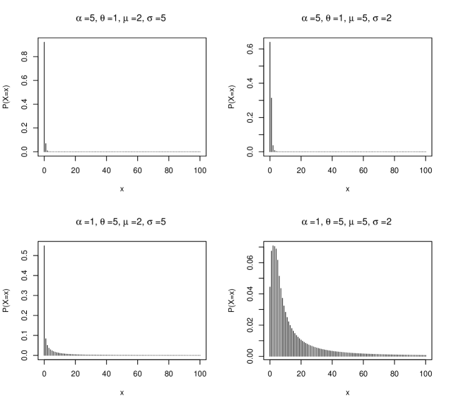
Figure 1: The PMF plot of DWLNP with different parameters

3.2 Weighted Discrete Weibull-Pareto (WDWP) Model

Suppose $X$ is a random variable that follows a weighted Weibull-Pareto (WWP) distribution that utilizes only the continuity condition in $x=\theta$. Then in Equation 3, we choose the pdf and CDF of Weibull distribution as $g_{1}$ and $G_{1}$.

$$\begin{cases}g_{1}(x)=(\frac{a}{\sigma})(\frac{x}{\sigma})^{a-1}e^{-(\frac{x}{\sigma})^{a}}\\[10.0pt] G_{1}(x)=1-e^{-(\frac{x}{\sigma})^{a}}\end{cases}$$

We also utilize Equation 5 as our selection for $g_{2}$ and $G_{2}$. Similar to $\phi$ parameter in the WWP model, a closed-form expression of $\phi$ in terms of all other parameters:

$$\phi(a,\sigma,\alpha,\theta)=\frac{a\theta^{a}e^{-\left(\frac{\theta}{\sigma}\right)^{a}}}{\alpha\sigma^{a}\left[1-e^{-\left(\frac{\theta}{\sigma}\right)^{a}}\right].}$$

The pdf of WWP can then be expressed as follows with 4 parameters:

$$f_{X}(x|a,\sigma,\alpha,\theta)=\begin{cases}\frac{1}{1+\phi(a,\sigma,\alpha,\theta)}\frac{(\frac{a}{\sigma})(\frac{x}{\sigma})^{a-1}e^{-(\frac{x}{\sigma})^{a}}}{1-e^{-(\frac{\theta}{\sigma})^{a}}}&x\in(0,\theta]\\[10.0pt] \frac{\phi(a,\sigma,\alpha,\theta)}{1+\phi(a,\sigma,\alpha,\theta)}\frac{\alpha\theta^{\alpha}}{x^{\alpha+1}}&x\in(\theta,\infty),\\ \end{cases}$$

The CDF of WWP can be derived as follows based on its definition:

$$F_{X}(x|a,\sigma,\alpha,\theta)=\begin{cases}0&x=0\\[10.0pt] \frac{1}{1+\phi(a,\sigma,\alpha,\theta)}\frac{1-e^{-(\frac{x}{\sigma})^{a}}}{1-e^{-(\frac{\theta}{\sigma})^{a}}}&x\in(0,\theta]\\[10.0pt] \frac{1+\phi(a,\sigma,\alpha,\theta)[1-(\frac{\theta}{x})^{\alpha}]}{1+\phi(a,\sigma,\alpha,\theta)}&x\in(\theta,\infty).\\ \end{cases}$$

The survival function of WWP can then be derived as:

$$S_{X}(x|a,\sigma,\alpha,\theta)=\begin{cases}1&x=0\\[10.0pt] 1-\frac{1}{1+\phi(a,\sigma,\alpha,\theta)}\frac{1-e^{-(\frac{x}{\sigma})^{a}}}{1-e^{-(\frac{\theta}{\sigma})^{a}}}&x\in(0,\theta]\\[10.0pt] 1-\frac{1+\phi(a,\sigma,\alpha,\theta)[1-(\frac{\theta}{x})^{\alpha}]}{1+\phi(a,\sigma,\alpha,\theta)}&x\in(\theta,\infty).\\ \end{cases}$$

Assume $Y$ is a random variable that follows WDWP distribution. Using the survival discretization method, the corresponding pmf of the WDWP model can be obtained as follows:

If $\theta\leq 1$:

$$P(Y=y)=\begin{cases}\frac{1+\phi(a,\sigma,\alpha,\theta)[1-\theta^{\alpha}]}{1+\phi(a,\sigma,\alpha,\theta)}&y=0\\[10.0pt] \frac{\phi(a,\sigma,\alpha,\theta)[(\frac{\theta}{y})^{\alpha}-(\frac{\theta}{y+1})^{\alpha}]}{1+\phi(a,\sigma,\alpha,\theta)}&y\in(0,\infty),\end{cases}$$ (10)

If $\theta>1$,

$$P(Y=y)=\begin{cases}\frac{e^{-(\frac{y}{\sigma})^{a}}-e^{-(\frac{y+1}{\sigma})^{a}}}{[1+\phi(a,\sigma,\alpha,\theta)][1-e^{-(\frac{\theta}{\sigma})^{a}}]}&y\in[0,\theta-1)\\[10.0pt] \frac{e^{-(\frac{y}{\sigma})^{a}}-e^{-(\frac{\theta}{\sigma})^{a}}+\phi(a,\sigma,\alpha,\theta)[1-e^{-(\frac{\theta}{\sigma})^{a}}][1-(\frac{\theta}{y+1})^{\alpha}]}{[1+\phi(a,\sigma,\alpha,\theta)][1-e^{-(\frac{\theta}{\sigma})^{a}}]}&y\in[\theta-1,\theta)\\[10.0pt] \frac{\phi(a,\sigma,\alpha,\theta)[(\frac{\theta}{y})^{\alpha}-(\frac{\theta}{y+1})^{\alpha}]}{1+\phi(a,\sigma,\alpha,\theta)}&y\in[\theta,\infty).\end{cases}$$ (11)

Similar to WDLNP model, $Y$ follows a discrete distribution with a heavy tail. The distribution of $Y$ has a fat tail when $\alpha<2$.

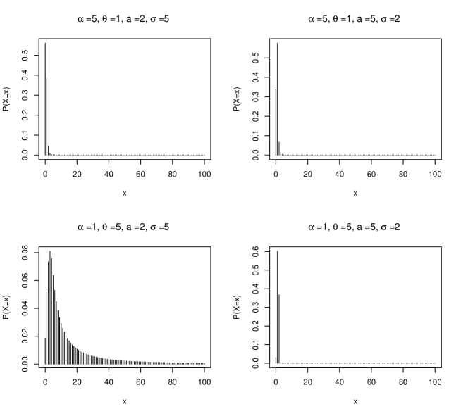
Figure 2: The PMF plot of DWWP with different parameters

3.3 The properties of the $n$-th moments for the discrete composite distributions with Pareto tails

In this subsection, important properties of the discrete composite distributions with Pareto tails are discussed in terms of $n$-th moments. As an analogue of continuous composite distributions with Pareto tails, we intend to formally show that the moments of discrete composite distributions with Pareto tails only exist under certain conditions.

Theorem 1

Suppose $Y$ is associated with a weighted discrete composite distribution with a Pareto tail, then the $n$-th moment of $Y$ does not exist if $\alpha\leq n$, where $\alpha$ is the shape parameter of the Pareto tail.

Suppose $Y$ follows a weighted discrete composite distribution created from Equation 2 with only the continuity condition, using the survival disretization method in 6. Then, the $n$-th moment of $Y$ can be written as follows:

$$\begin{split}E(Y^{n})&=\sum_{y\in\mathbb{N}_{0},y<\theta}y^{n}P(Y=y|Y<\theta)+\sum_{y\in\mathbb{N}_{0},y\geq\theta}y^{n}P(Y=y|Y\geq\theta)\\ &\geq\sum_{y\in\mathbb{N}_{0},y\geq\theta}y^{n}P(Y=y|Y\geq\theta),\end{split}$$

where $\theta$ is the parameter that determines the change of density in a composite distribution.

Notice for any discrete composite random variable $Y$ with a Pareto($\alpha,\theta$) tail that created based on a continuous composite distribution with the survival dicretization method, we have the following:

$$P(Y=y|Y\geq\theta)=\frac{\phi[(\frac{\theta}{y})^{\alpha}-(\frac{\theta}{y+1})^{\alpha}]}{1+\phi},$$

where $\phi$ is uniquely determined by other parameters of the model.

Then,

$$\begin{split}\sum_{y\in\mathbb{N}_{0},y\geq\theta}y^{n}P(Y=y|Y\geq\theta)&=\sum_{y\in\mathbb{N}_{0},y\geq\theta}y^{n}\frac{\phi[(\frac{\theta}{y})^{\alpha}-(\frac{\theta}{y+1})^{\alpha}]}{1+\phi}\\ &=\frac{\phi\theta^{\alpha}}{1+\phi}\sum_{y\in\mathbb{N}_{0},y\geq\theta}\left[y^{n-\alpha}-y^{n}(y+1)^{-\alpha}\right]\\ &\geq\frac{\phi\theta^{\alpha}}{1+\phi}\sum_{y\in\mathbb{N}_{0},y\geq\theta}\left[y^{n-\alpha}-(y+1)^{n-\alpha}\right]\\ &=\frac{\phi\theta^{\alpha}}{1+\phi}\left[{\lceil\theta\rceil}^{n-\alpha}-\lim_{y\rightarrow\infty}(y+1)^{n-\alpha}\right],\end{split}$$

where $\lceil\theta\rceil$ is the least integer greater or equal to $\theta$. Notice $\lim_{y\rightarrow\infty}(y+1)^{n-\alpha}$ is infinite if $n-\alpha\geq 0$. Therefore, the $n$-th moment does not exist for $Y$ if $\alpha\leq n$. As a consequence, we have the following two corollaries:

Corollary 1

Suppose $Y$ is associated with a weighted discrete composite distribution with a Pareto tail, the mean of $Y$ does not exist if $\alpha\leq 1$.

Corollary 2

Suppose $Y$ is associated with a weighted discrete composite distribution with a Pareto tail, the variance of $Y$ does not exist if $\alpha\leq 2$.

In fact, for some special choices of parameters, we are able to derive the moment explicitly. For example, when $\alpha>1$ and $\theta\leq 1$, we can derive the following:

Theorem 2

Suppose $Y$ follows a weighted discrete composite distribution with a Pareto tail. Assume $\alpha>1$ and $\theta\leq 1$. The mean of $Y$ is equal to $\frac{\phi\theta^{\alpha}}{1+\phi}\zeta(\alpha)$, where $\zeta(.)$ stands for a Riemann zeta function.

Suppose $\theta\leq 1$ and $\alpha>1$, then we have the following:

$$\begin{split}E(Y)&=\sum_{y\in\mathbb{N}_{0},y<\theta}yP(Y=y|Y<\theta)+\sum_{y\in\mathbb{N}_{0},y\geq\theta}y^{n}P(Y=y|Y\geq\theta)\\ &=\sum_{y^{n}\in\mathbb{N}_{0},y\geq\theta}yP(Y=y|Y\geq\theta)\\ &=\sum_{y=1}^{\infty}yP(Y=y|Y\geq\theta)\\ &=\sum_{y=1}^{\infty}y\frac{\phi[(\frac{\theta}{y})^{\alpha}-(\frac{\theta}{y+1})^{\alpha}]}{1+\phi}\\ &=\frac{\phi\theta^{\alpha}}{1+\phi}\sum_{y=1}^{\infty}\left[y^{1-\alpha}-y(y+1)^{-\alpha}\right]\\ &=\frac{\phi\theta^{\alpha}}{1+\phi}\left[1+\sum_{y=2}^{\infty}y^{1-\alpha}-\sum_{y=2}^{\infty}(y-1)y^{-\alpha}\right]\\ &=\frac{\phi\theta^{\alpha}}{1+\phi}\left(1+\sum_{y=2}^{\infty}\frac{1}{y^{\alpha}}\right)\\ &=\frac{\phi\theta^{\alpha}}{1+\phi}\left(\sum_{y=1}^{\infty}\frac{1}{y^{\alpha}}\right)\\ &=\frac{\phi\theta^{\alpha}}{1+\phi}\zeta(\alpha)\end{split}$$

Since $\zeta(2)=\frac{\pi^{2}}{6}$, we have the following:

Suppose $Y$ follows a weighted discrete composite distribution with a Pareto tail. Suppose $\theta\leq 1$ and $\alpha=2$. The mean of $Y$ is equal to $\frac{\pi^{2}\phi\theta^{2}}{6(1+\phi)}$

In the next section, the inference on the scale parameter $\alpha$ will be introduced based on properties we discussed in this section.

4 Estimation and Hypothesis Testing

In this section, the parameter estimation of the discrete composite distributions and the hypothesis testing procedures of the tail index will be introduced.

4.1 Estimation

Given a particular data set, the parameters the discrete composite distributions with Pareto tails can be estimated with maximum likelihood estimation. Suppose $y_{1},y_{2},...,y_{n}$ is a random sample of size $n$ that follows a weighted discrete composite distribution with a Pareto tail. For different $\theta$ values, the likelihood can be written as follows:

1. When $\theta\leq 1$, the pmf of $y_{i}$ can be written as follows:

   $$P(Y=y_{i})=\begin{cases}\frac{1+\phi(\boldsymbol{\beta_{1}},\alpha,\theta)[1-\theta^{\alpha}]}{1+\phi(\boldsymbol{\beta_{1}},\alpha,\theta)}&y_{i}=0\\[10.0pt] \frac{\phi(\boldsymbol{\beta_{1}},\alpha,\theta)[(\frac{\theta}{y_{i}})^{\alpha}-(\frac{\theta}{y_{i}+1})^{\alpha}]}{1+\phi(\boldsymbol{\beta_{1}},\alpha,\theta)}&y_{i}\in(0,\infty),\end{cases}$$

   where $\alpha$ and $\theta$ are the parameters of the Pareto tail; $\boldsymbol{\beta_{1}}$ is the parameter vector for the distribution selected as the head in a weighted discrete composite distribution. Then, the corresponding log-likelihood $l_{1}$ can be expressed as follows:

   $$l_{1} =-n\text{ln}[1+\phi(\boldsymbol{\beta_{1}},\alpha,\theta)]+\sum_{i=1}^{m}\text{ln}\left\{1+\phi(\boldsymbol{\beta_{1}},\alpha,\theta)(1-\theta^{\alpha})\right\}$$

   $$+\sum_{y_{i}>0}\text{ln}\left\{\phi(\boldsymbol{\beta_{1}},\alpha,\theta)[(\frac{\theta}{y_{i}})^{\alpha}-(\frac{\theta}{y_{i}+1})^{\alpha}]\right\},$$

   where $m=\sum_{i=1}^{n}I(y_{i}=0)$ and $I(.)$ stands for the indicator function.

2. When $\theta>1$, the pmf of $y_{i}$ can be represented as follows:

   $$P(Y=y)=\begin{cases}\frac{G_{1}(y+1|\boldsymbol{\beta_{1}})-G_{1}(y|\boldsymbol{\beta_{1}})}{[1+\phi(\boldsymbol{\beta_{1}},\alpha,\theta)][G_{1}(\theta|\boldsymbol{\beta_{1}})]}&y\in[0,\theta-1)\\[10.0pt] \frac{G_{1}(\theta|\boldsymbol{\beta_{1}})-G_{1}(y|\boldsymbol{\beta_{1}})+\phi(\boldsymbol{\beta_{1}},\alpha,\theta)[G_{1}(\theta|\boldsymbol{\beta_{1}})][1-(\frac{\theta}{y+1})^{\alpha}]}{[1+\phi(\boldsymbol{\beta_{1}},\alpha,\theta)][G_{1}(\theta|\boldsymbol{\beta_{1}})]}&y\in[\theta-1,\theta)\\[10.0pt] \frac{\phi(\boldsymbol{\beta_{1}},\alpha,\theta)[(\frac{\theta}{y})^{\alpha}-(\frac{\theta}{y+1})^{\alpha}]}{1+\phi(\boldsymbol{\beta_{1}},\alpha,\theta)}&y\in[\theta,\infty),\end{cases}$$

   where $G_{1}$ is the cdf of the distribution selected as the head.

   Thus, the corresponding log-likelihood $l_{2}$ can be represented as follows:

   $$l_{2} =-n\text{ln}[1+\phi(\boldsymbol{\beta_{1}},\alpha,\theta)]+\sum_{y_{i}<\theta-1}\text{ln}\left[G_{1}(y_{i}+1|\boldsymbol{\beta_{1}})-G_{1}(y_{i}|\boldsymbol{\beta_{1}})\right]$$

   $$+\sum_{\theta-1\leq y_{i}<\theta}\text{ln}\left\{G_{1}(\theta|\boldsymbol{\beta_{1}})-G_{1}(y_{i}|\boldsymbol{\beta_{1}})+\phi(\boldsymbol{\beta_{1}},\alpha,\theta)[G_{1}(\theta|\boldsymbol{\beta_{1}})][1-(\frac{\theta}{y_{i}+1})^{\alpha}]\right\}$$

   $$-(m_{1}+m_{2})\text{ln}[G_{1}(\theta|\boldsymbol{\beta_{1}})]+\sum_{y_{i}\geq\theta}\text{ln}\left\{\phi(\boldsymbol{\beta_{1}},\alpha,\theta)[(\frac{\theta}{y_{i}})^{\alpha}-(\frac{\theta}{y_{i}+1})^{\alpha}]\right\},$$

where $m_{1}=\sum_{i=1}^{n}I(y_{i}<\theta-1)$ and $m_{2}=\sum_{i=1}^{n}I(\theta-1\leq y_{i}<\theta)$.

Eventually, the log-likelihood of $y_{1},y_{2},...,y_{n}$ can be represented as follows with $l_{1}$ and $l_{2}$ we just derived:

$$l(\boldsymbol{\beta_{1}},\alpha,\theta|y_{1},y_{2},...,y_{n})=I(\theta\leq 1)l_{1}+[1-I(\theta\leq 1)]l_{2}.$$ (12)

The maximum likelihood estimates (MLE) of the parameters are as follows:

$$(\hat{\boldsymbol{\beta_{1}}},\hat{\alpha},\hat{\theta})=\operatorname*{arg\,max}_{\boldsymbol{\beta_{1}},\alpha,\theta}l(\boldsymbol{\beta_{1}},\alpha,\theta|y_{1},y_{2},...,y_{n})$$

Clearly, the MLE of the parameters cannot be obtained with an analytical form. With the ’optim’ function in R, we can obtain the MLE numerically.

4.2 Testing of the shape parameter $\alpha$

In Section 3, it is shown that the moment a discrete composite random variable with a Pareto tail does not exist when $\alpha\leq 1$. We also show that the variance of a discrete composite random variable with a Pareto tail does not exist when $\alpha\leq 2$. Numerically, we are able to find the MLE of $\alpha$ by maximizing the loglikelihood in Equation 12. In addition to the sole point estimate of $\alpha$, hypothesis testing of the shape parameter $\alpha$ can be quite helpful in addition to the sole point estimate of $\alpha$ in real data applications to the infectious disease counting data. Essentially, the null hypotheses of interest are as follows:

1. $H_{0}:\alpha\leq 1$ (Test for infinite mean)

2. $H_{0}:\alpha\leq 2$ (Test for infinite variance)

In order to test the above hypotheses, the likelihood ratio test (LRT) can be used. Assume that the loglikelihood function $l(\boldsymbol{\beta_{1}},\alpha,\theta|y_{1},y_{2},...,y_{n})$ takes the form in Equation 12. For the simplicity of the expression, let $\Pi=(\boldsymbol{\beta_{1}},\alpha,\theta)$ and $\boldsymbol{y}=(y_{1},y_{2},...,y_{n})$. Let $S$ be the parameter space of $\Pi$ and $S_{0}$ be the parameter space of $\Pi$ when $H_{0}$ is true. The LRT statistic $\lambda$ for the given hypothesis is as follows:

$$\centering\lambda=2\text{sup}_{\Pi\in S}l(\Pi|\boldsymbol{y})-2{\text{sup}_{\Pi\in S_{0}}l(\Pi|\boldsymbol{y})},\@add@centering$$ (13)

where $\lambda$ follows a $\chi^{2}$ distribution with a degree of freedom 1 asymptotically. The corresponding p-value of the test is $P(\chi^{2}_{1}>\lambda)$. $H_{0}$ shall be rejected when the p-value is less than the prespecified significance level.

5 Applications

In this section, the two novel discrete composite distributions are applied to two different infectious disease data sets. For comparison purposes, we also analyze the data sets with four well-known parametric models: Poisson, zero-inflated Poisson (ZIP), negative binomial (NB), and zero-inflated negative binomial (ZINB). To evaluate model performance, we use the Akaike Information Criteria (AIC) [26]. AIC is defined as follows :

$AIC=-2l+2k$,

where $l$ denotes the loglikelihood. $k$ denotes the number of free parameters. A model with the lowest AIC value is considered a preferred fit when compared to all the chosen models.

In addition, we also utilize the hypothesis testing procedures in 4.2 to provide statistical inference of the tail index parameter for the two discrete composite distributions with Pareto tails.

Case 1: COVID-19 Outbreak: Singapore

Data Description and Analysis Plan

To evaluate the performance of the new discrete composite distributions, the COVID-19 data set on WHO website was utilized. The data set is publicly available at https://covid19.who.int/data. The numbers of reported cases by days in Singapore from April 1st, 2021 to January 1st, 2023 were included in our analysis. The time series for the daily count of cases is presented in Figure 3. We first analyze the reported cases from the first three months (4/1/2021-7/1/2021). Then, we update our analysis by incorporating the cases from the next three months. In a sequential manner, we were able to obtain the analysis results on seven particular dates: 7/1/2021, 10/1/2021, 1/1/2022, 4/1/2022, 7/1/2022, 10/1/2022, and 1/1/2023.

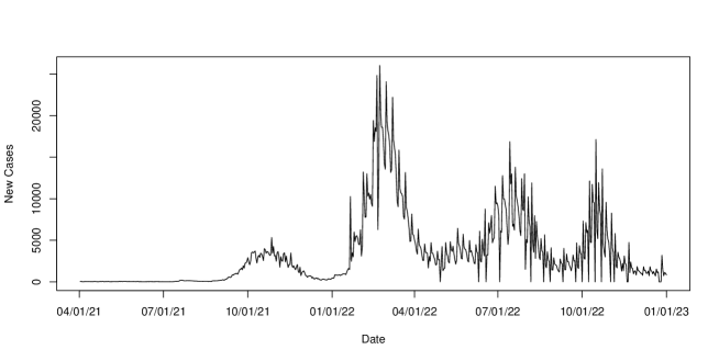
Figure 3: The COVID-19 cases over time in Singapore from 04/2021 to 01/2023

Results

Table 1 shows the AIC values for six different models on seven particular dates. Models with the lowest AIC values were highlighted in red. For the dates 10/1/2021, 04/1/2022, 10/1/2022, and 1/1/2023, we noticed that new discrete composite models (WDLNP and WDWP) can provide better performance compared to other well-known models. Figure 4 shows the estimated CDF plot with two discrete composite models with the empirical CDF when we included all daily reported count cases from 4/1/2021 to 1/1/2023. Both models demonstrated great ability in fitting the data, especially at the upper tail.

Figure 5 demonstrates the change of $\alpha$ estimates over time for two discrete composite models. The black horizontal dashed line stands for $\alpha=2$, and the blue horizontal dashed line represents $\alpha=1$. Note for both models, the $\alpha$ estimates are less than $1$ during 10/1/2021 and 04/01/2022. Table 2 and 3 shows the results of the hypothesis testing for the tail index parameter $\alpha$ for two models. During 10/1/2021 and 04/01/2022, we notice that the null hypothesis of $\alpha=1$ and $\alpha=2$ should not be rejected for both models at the significance level of 0.05. This suggests that during this period of time, the estimated mean and variance of the case counts for both models are likely to be infinite. On 7/1/2022, only $\alpha=1$ should be rejected for both models. This implies that the mean of the case counts is now finite, but still likely to be associated with infinite variance. On 10/1/2022 and 1/1/2023, both null hypothesis for the tail index should be rejected for the WDWP model. The $p$-value of testing $\alpha=2$ for the WDLNP model is inconclusive on 10/1/2022. However, both null hypothesis should be rejected at the level of 0.05 for the WDLNP model.

If we examine the results from Figure 5, Table 2, and Table 3 together with the time series plot in 3, we are able to get a general understanding about the severity of pandemic in Singapore in terms of case counts. The COVID-19 pandemic became a major public health problem in Singapore during 10/1/2021 and 4/1/2022, as the tail index estimates $\alpha$ are below 1. On 7/1/2022, although the estimate of $\alpha$ is beyond 2 for both composite models, we cannot still reject $\alpha\leq 2$ based on the LRT test. This implies it is still very likely to see rare but extremely large number of counts of cases on a single day. The local hospitals and public health agencies should still be alert to very large counts. From 10/1/2022, although we still see a considerable amount of reported cases in Figure 3, we have gained more evidence that $\alpha\leq 2$ will be rejected for both models. Essentially, this implies that the local health agencies were likely to be prepared for these new cases, since they have already survived from a higher peak of reported cases.

Table 1: AIC values for six different models (COVID cases in Singapore: 4/1/2021-1/1/2023)

	Poisson	ZIP2	NB3	ZINB4	WDLNP5	WDWP6
Date1
7/1/2021	846.8136	848.8143	683.1605	685.1605	691.7478	689.6392
10/1/2021	101068.4	101070.4	2252.341	2254.341	2096.286	2096.432
1/1/2022	416336.8	416338.8	4027.38	4029.38	3967.172	3967.144
4/1/2022	2249692	2249694	6092.806	6094.806	6050.2	6079.752
7/1/2022	2366642	2366644	7850.405	7852.405	7856.288	7854.078
10/1/2022	2706326	2706328	9610.242	9612.242	9603.92	9605.378
1/1/2023	2995122	2859516	11245.88	11244.79	11231.17	11239.7

¹ The data was included from 4/1/2021 until this date.
² Zero-inflated Poisson
³ Negative binomial
⁴ Zero-inflated negative binomial

⁵ Weighted discrete lognormal-Pareto
⁶ Weighted discrete Weibull-Pareto

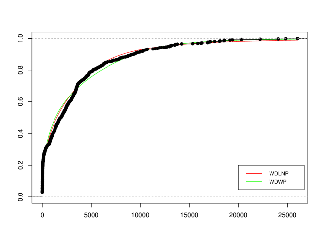
Figure 4: The empirical CDF of COVID-19 cases in Singapore from 4/1/2021 to 1/1/2023 with the fitted CDF of two discrete composite distributions

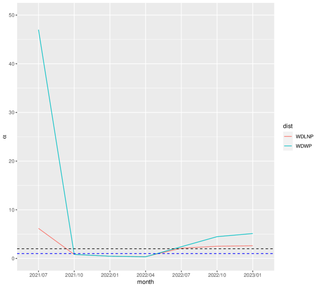
Figure 5: The change of $\alpha$ estimates over time for two composite models when fitting to the COVID-19 cases data from Singapore

Table 2: The LRT test results for tail index $\alpha$ with WDLNP model when fitting to COVID-19 cases in Singapore

Date	$\boldsymbol{H_{0}:\alpha\leq 1}$		$\boldsymbol{H_{0}:\alpha\leq 2}$
	$\chi^{2}$ Statistic	p-value	$\chi^{2}$ Statistic	p-value
7/1/2021	77.52	$1.31\times 10^{-18}$	28.79	$8.05\times 10^{-8}$
10/1/2021	0	1	0	1
1/1/2022	0	1	0	1
4/1/2022	$4.85\times 10^{-8}$	1	0	1
7/1/2022	48.81	$2.82\times 10^{-12}$	0.37	0.54
10/1/2022	70.38	$4.89\times 10^{-17}$	3.49	0.06
1/1/2023	85.59	$2.22\times 10^{-20}$	5.98	0.01

Table 3: The LRT test results for tail index $\alpha$ with WDWP model when fitting to COVID-19 cases in Singapore

Date	$\boldsymbol{H_{0}:\alpha\leq 1}$		$\boldsymbol{H_{0}:\alpha\leq 2}$
	$\chi^{2}$ Statistic	p-value	$\chi^{2}$ Statistic	p-value
7/1/2021	79.62	$4.54\times 10^{-19}$	30.90	$2.72\times 10^{-8}$
10/1/2021	$4.70\times 10^{-5}$	0.99	0	1
1/1/2022	$3.36\times 10^{-7}$	1	0	1
4/1/2022	0	1	0	1
7/1/2022	41.48	$1.19\times 10^{-10}$	1.92	0.17
10/1/2022	74.65	$5.63\times 10^{-18}$	11.35	$7.53\times 10^{-4}$
1/1/2023	111.87	$3.82\times 10^{-26}$	28.45	$9.62\times 10^{-8}$

Case 2: Monkeypox Outbreak 2022: France

Data Description and Analysis Plan

We also used the monkeypox (mpox) data set on Our World In Data [27] to assess the performance of new discrete composite models. The numbers of reported cases by days in France from May 19st, 2022 to January 1st, 2023 were included in our analysis. The time series for daily cases count is presented in Figure 3. Unlike the COVID-19 data set we chose in case 1, this data set contains a considerable amount of zeros. We first analyze the reported cases from May 19st, 2022 to July 1st, 2022. Then, we update our analysis by incorporating the cases from next month. Sequentially, we were able to obtain the analysis results on seven particular dates: 7/1/2022, 8/1/2021, 9/1/2022, 10/1/2022, 11/1/2022, 12/1/2022, and 1/1/2023.

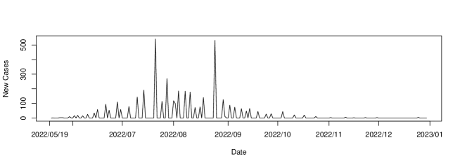
Figure 6: The mpox cases over time in France from 5/19/2022 to 01/01/2023

Results

Table 4 shows the AIC values for six different models on seven particular dates. Models with the lowest AIC values were highlighted in red. For the dates 7/1/2022, 9/1/2022, 10/1/2022, and 11/1/2022, the discrete composite models demonstrated better performance compared to well-known models. Figure 7 presents the estimated CDF plot with two discrete composite models with the empirical CDF when we included all the daily reported count cases from 5/19/2022 to 1/1/2023. Both models demonstrated reasonably good performance when to fitting to upper tail. However, both lognormal and Weibull distribution cannot capture the lower tail features of the data well based on Figure 7. This suggest better choices of the head distributions for the discrete composite models might exist when fitting to the data set.

Table 4: AIC Values for Different Models (Mpox Cases in France: 5/19/2022-1/1/2023)

	Poisson	ZIP2	NB3	ZINB4	WDLNP5	WDWP6
Date1
7/1/2022	1629.815	681.9589	200.2278	201.1567	200.1003	209.1702
8/1/2022	7512.623	2985.267	340.0716	342.4696	341.7540	342.6394
9/1/2022	12538.09	4367.755	514.1144	516.1153	512.073	514.2812
10/1/2022	14133.59	4906.265	647.5542	649.5543	643.7592	646.7542
11/1/2022	15626.52	5267.969	715.6079	717.608	711.1758	713.905
12/1/2022	16918.46	5880.85	766.7535	760.442	763.0148	765.2526
1/1/2023	18088.32	6173.418	801.2655	796.9182	797.7298	799.452

¹ The data was included from 5/19/2022 until this date.
² Zero-inflated Poisson
³ Negative binomial
⁴ Zero-inflated negative binomial

⁵ Weighted discrete lognormal-Pareto
⁶ Weighted discrete Weibull-Pareto

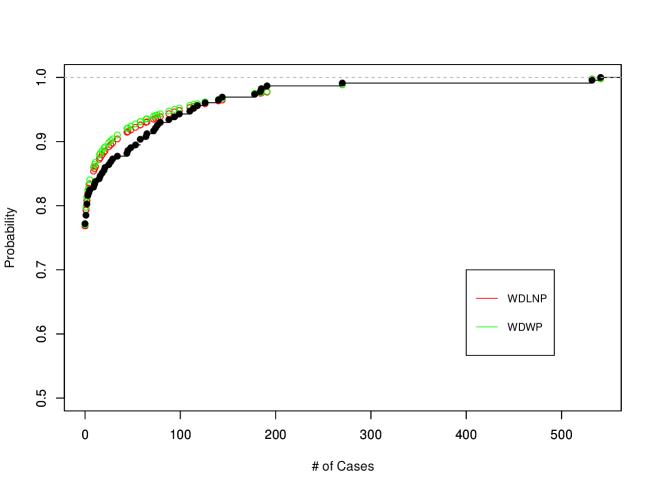
Figure 7: The empirical CDF of mpox cases in France from 5/19/2022 to 1/1/2023 with the fitted CDF of two composite distributions

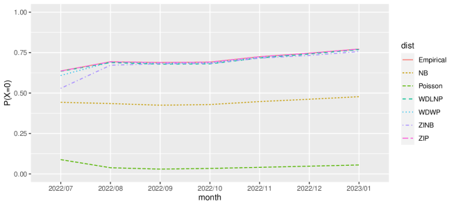
Figure 8: The estimated probability of $0$ cases for different models

Figure 8 shows the estimated probability for zero cases for different models when fitting to the mpox data. In terms of the ability to capture the probability of zero cases, our model can demonstrate comparable performance to that of zero-inflated models without adding a parameter for modeling the probability of zero cases.

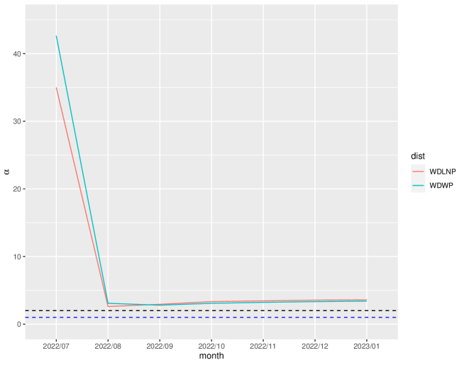
Figure 9: The change of $\alpha$ estimates over time for two composite models when fitting to the mpox data from France

Figure 9 demonstrates the change of $\alpha$ estimates over time for two discrete composite models. Again, the black horizontal dashed line stands for $\alpha=2$, and the blue horizontal dashed line represents $\alpha=1$. Note for both models, the $\alpha$ estimates are greater than $2$ during 7/1/2021 and 01/01/2022. Table 5 and 6 shows the results of the hypothesis testing for the tail index parameter $\alpha$ for two models. We notice that only for the date 8/1/2022, the null hypothesis of $\alpha=1$ should not be rejected for both models at the significance level of 0.05. This suggests that the estimated expected counts of cases for both models are finite for most of the scenarios. However, during the whole observation period, $\alpha=2$ should not be rejected for both models at the significance level of 0.05. This the counts were possibly associated with infinite variance, even the estimates of $\alpha$ are over 2 for the whole time.

Similar to the analysis we did for the COVID-19 cases in Singapore, we can view the results from Figure 9, Table 5, and Table 6 with the time series plot in Figure 6 for the mpox cases in France. Notice we reject both $\alpha\leq 1$ and $\alpha\leq 2$ on 7/1/2022 as the estimated mean and variance are expected to be finite. This implies mpox should not be considered as a major public health concern at that time. On 8/1/2022, the $\alpha$ estimates for both models drops to nearly 2 and the LRT suggests that the null hypothesis of infinite mean and variance should not be rejected. This makes sense since we saw the large number of reported cases in July and local health agencies should plan for extremely high counts in mpox cases. However, even though some new cases were reported in August or September, they did not cause drastic changes in the estimate of $\alpha$ for both models. The $\alpha$ estimates for the dates after 8/1/2022 stayed beyond 2 until 1/1/2023. This suggests the mpox outbreak in France was in a controllable situation after the first wave of reported cases.

Table 5: The LRT test results for tail index $\alpha$ with WDLNP model when fitting to mpox data in France

Date	$\boldsymbol{H_{0}:\alpha\leq 1}$		$\boldsymbol{H_{0}:\alpha\leq 2}$
	$\chi^{2}$ Statistic	p-value	$\chi^{2}$ Statistic	p-value
7/1/2022	5.77	0.02	3.60	0.06
8/1/2022	2.57	0.11	0.15	0.70
9/1/2022	4.93	0.03	0.94	0.33
10/1/2022	5.94	0.02	1.10	0.29
11/1/2022	6.15	0.01	1.10	0.29
12/1/2022	6.26	0.01	1.09	0.30
1/1/2023	6.29	0.01	1.03	0.31

Table 6: The LRT test results for tail index $\alpha$ with WDWP model when fitting to mpox data in France

Date	$\boldsymbol{H_{0}:\alpha\leq 1}$		$\boldsymbol{H_{0}:\alpha\leq 2}$
	$\chi^{2}$ Statistic	p-value	$\chi^{2}$ Statistic	p-value
7/1/2022	4.74	0.03	2.54	0.11
8/1/2022	2.43	0.12	0.29	0.59
9/1/2022	4.36	0.04	0.72	0.40
10/1/2022	3.85	0.05	1.10	0.29
11/1/2022	5.84	0.02	1.19	0.28
12/1/2022	5.99	0.01	1.19	0.27
1/1/2023	6.04	0.01	1.17	0.28

6 Concluding Remarks

In this paper, we introduced the new discrete composite distributions with Pareto tails. We created two novel discrete composite distributions named weighted discrete lognormal-Pareto distribution (WDLNP) and weighted discrete Weibull-Pareto distribution (WDWP). Some properties about the new distributions were derived. In addition, we developed a testing procedure to test the hypotheses of infinite mean and infinite variance of the discrete composite models. Two novel discrete composite models can provide very good performance when fitting to real infectious disease data. We also justified the capability of these two models when fitting to the data with excess zeros by using real data.

The findings from the real data application are interesting. As Poisson distribution is widely used in modeling the cases of infectious diseases, it demonstrated poor performance when fitting to both real data sets we selected. Like some previous literature suggested [2], Poisson distribution does not perform well when the data is characterized with heavy-tailed features. As a comparison, our models demonstrated great and consistent performance when fitting to two different infectious diseases data sets due to the Pareto tail we selected. In addition, the estimated Pareto tail index parameter of these models can provide us a way to monitor the severity of the an infectious disease in terms of reported cases. As we showed in two real data examples, we were able to sequentially update our models and testing results by incorporating new cases reported. By tracing the change of tail index parameter and hypothesis testing results, we were able to provide a way to monitor the progression of a pandemic such as COVID-19.

References

- Brown et al. [2021] M. Brown, J. E. Cohen, C.-F. Tang, S. C. P. Yam, Taylor’s law of fluctuation scaling for semivariances and higher moments of heavy-tailed data, Proceedings of the National Academy of Sciences 118 (2021) e2108031118. Publisher: Proceedings of the National Academy of Sciences.
- Cohen et al. [2022] J. E. Cohen, R. A. Davis, G. Samorodnitsky, COVID-19 cases and deaths in the United States follow Taylor’s law for heavy-tailed distributions with infinite variance, Proceedings of the National Academy of Sciences 119 (2022) e2209234119. Publisher: Proceedings of the National Academy of Sciences.
- Beare and Toda [2020] B. K. Beare, A. A. Toda, On the emergence of a power law in the distribution of COVID-19 cases, Physica D. Nonlinear Phenomena 412 (2020) 132649.
- Blasius [2020] B. Blasius, Power-law distribution in the number of confirmed COVID-19 cases, Chaos 30 (2020) 093123.
- Cooray and Ananda [2005] K. Cooray, M. M. A. Ananda, Modeling actuarial data with a composite lognormal-pareto model, Scandinavian Actuarial Journal 2005 (2005) 321–334.
- Scollnik [2007] D. P. M. Scollnik, On composite lognormal-Pareto models, Scandinavian Actuarial Journal 2007 (2007) 20–33.
- Scollnik and Sun [2012] D. P. M. Scollnik, C. Sun, Modeling with weibull-pareto models, North American Actuarial Journal 16 (2012) 260 – 272.
- Brazauskas and Kleefeld [2016] V. Brazauskas, A. Kleefeld, Modeling Severity and Measuring Tail Risk of Norwegian Fire Claims, North American Actuarial Journal 20 (2016) 1–16.
- Grün and Miljkovic [2019] B. Grün, T. Miljkovic, Extending composite loss models using a general framework of advanced computational tools, Scandinavian Actuarial Journal 2019 (2019) 642–660.
- Liu and Ananda [2022a] B. Liu, M. M. A. Ananda, Analyzing insurance data with an exponentiated composite Inverse-Gamma Pareto Model, Communications in Statistics - Theory and Methods (2022a).
- Liu and Ananda [2022b] B. Liu, M. M. A. Ananda, A Generalized Family of Exponentiated Composite Distributions, Mathematics 10 (2022b) 1895. Number: 11 Publisher: Multidisciplinary Digital Publishing Institute.
- Mutali and Vernic [2020] S. Mutali, R. Vernic, On the composite Lognormal–Pareto distribution with uncertain threshold, Communications in Statistics - Simulation and Computation 0 (2020) 1–17. Publisher: Taylor & Francis.
- Deng and Aminzadeh [2019] M. Deng, M. S. Aminzadeh, Bayesian predictive analysis for Weibull-Pareto composite model with an application to insurance data, Communications in Statistics - Simulation and Computation 0 (2019) 1–27.
- Aminzadeh and Deng [2019] M. S. Aminzadeh, M. Deng, Bayesian predictive modeling for inverse gamma-pareto composite distribution, Communications in Statistics - Theory and Methods 48 (2019) 1938–1954.
- Nadarajah [2005] S. Nadarajah, Exponentiated pareto distributions, Statistics 39 (2005) 255–260.
- Calderín-Ojeda [2018] E. Calderín-Ojeda, A Note on Parameter Estimation in the Composite Weibull–Pareto Distribution, Risks 6 (2018) 11.
- Cooray [2009] K. Cooray, The Weibull–Pareto Composite Family with Applications to the Analysis of Unimodal Failure Rate Data, Communications in Statistics - Theory and Methods 38 (2009) 1901–1915.
- Cooray et al. [2010] K. Cooray, S. Gunasekera, M. Ananda, Weibull and inverse Weibull composite distribution for modeling reliability data, MAS 5 (2010) 109–115.
- Liu and Ananda [2023] B. Liu, M. M. A. Ananda, A New Insight into Reliability Data Modeling with an Exponentiated Composite Exponential-Pareto Model, Applied Sciences 13 (2023) 645. Number: 1 Publisher: Multidisciplinary Digital Publishing Institute.
- Chakraborty [2015] S. Chakraborty, Generating discrete analogues of continuous probability distributions-A survey of methods and constructions, Journal of Statistical Distributions and Applications 2 (2015) 6.
- Kemp [2004] A. W. Kemp, Classes of Discrete Lifetime Distributions, Communications in Statistics - Theory and Methods 33 (2004) 3069–3093. Publisher: Taylor & Francis.
- Roy [2003] D. Roy, The Discrete Normal Distribution, Communications in Statistics - Theory and Methods 32 (2003) 1871–1883.
- Abu Bakar et al. [2015] S. Abu Bakar, N. Hamzah, M. Maghsoudi, S. Nadarajah, Modeling loss data using composite models, Insurance: Mathematics and Economics 61 (2015) 146–154.
- Almetwally et al. [2022] E. M. Almetwally, D. A. Abdo, E. Hafez, T. M. Jawa, N. Sayed-Ahmed, H. M. Almongy, The new discrete distribution with application to COVID-19 Data, Results in Physics 32 (2022) 104987.
- Almetwally et al. [2023] E. M. Almetwally, S. Dey, S. Nadarajah, An Overview of Discrete Distributions in Modelling COVID-19 Data Sets, Sankhya A 85 (2023) 1403–1430.
- Burnham and Anderson [2002] K. P. Burnham, D. R. Anderson, Model Selection and Multimodel Inference, 2 ed., Springer-Verlag, 2002.
- Mathieu et al. [2022] E. Mathieu, F. Spooner, S. Dattani, H. Ritchie, M. Roser, Mpox (monkeypox), Our World in Data (2022). Https://ourworldindata.org/monkeypox.