Two-point spectroscopy of Fibonacci topoelectrical circuits

Abstract

Topoelectrical circuits are meta-material realizations of topological features of condensed matter systems. In this work, we discuss experimental methods that allow a fast and straightforward detection of the spectral features of these systems from the two-point impedance of the circuit. This allows to deduce the full spectrum of a topoelectrical circuit consisting of $N$ sites from a single two-point measurement of the frequency resolved impedance. In contrast, the standard methods rely on $N^{2}$ measurements of admittance matrix elements with a subsequent diagonalization on a computer. We experimentally test our approach by constructing a Fibonacci topoelectrical circuit. Although the spectrum of this chain is fractal, i.e., more complex than the spectra of periodic systems, our approach is successful in recovering its eigenvalues. Our work promotes the topoelectrical circuits as an ideal platform to measure spectral properties of various (quasi)crystalline systems.

Introduction — Experimental difficulties in realizing and detecting topological features of condensed-matter systems have prompted the development of meta-materials — classical systems designed to reproduce desired topological features. The initial proposal [1] involved photonic crystals where electromagnetic waves propagate unidirectionally along the boundary, thus forming the photonic analog of the integer quantum Hall effect (IQHE) [2]. In addition to photonic meta-materials [3, 4, 5, 6, 7, 8, 9, 10], there are acoustic [11, 12, 13, 14, 15, 16, 17, 18], mechanical [19, 20, 21], microwave [22, 23, 24, 25, 26, 27] and electrical circuit [28, 29, 30, 31, 32, 33, 34, 35, 36, 37, 38, 39, 40, 41, 42, 43, 44] realizations of various topological phases of matter.

Topoelectrical circuits are networks of nodes connected by electronic components such as resistors, capacitors, and inductors. They are described by an admittance matrix $Y(f)$ that represents the current response to a set $\textbf{V}(f)$ of locally applied voltages at frequency $f$, and that can be mapped to an effective tight-binding Hamiltonian [30, 45, 36]. So far, the experimental characterization of these classical systems mostly relied on detecting topological boundary phenomena using two-point impedance measurements [30, 45]. This impedance, $Z_{a,b}(f)$, can be determined by measuring the voltage response between the nodes $a$ and $b$ to an input current oscillating at a specific frequency. If this frequency corresponds to the energy of a topological boundary state of the effective Hamiltonian, and if the nodes are chosen such that one is in the bulk and the other in the region where this topological state is localized, the resulting two-point impedance is very large in realistic systems (it even diverges for ideal ones). Thus, the presence of a topological boundary state inside of the bulk gap results in a single, isolated impedance peak.

Gaining access to the full spectrum of the effective Hamiltonian simulated by a topoelectrical circuit, beyond the detection of individual, spectrally isolated modes, is challenging. The spectra of topoelectrical circuits have so far been determined by measuring the full admittance matrix, element by element, and then diagonalizing it on a computer [46]. This is a time-consuming process, since the number of measurements scales quadratically with the number of sites in the system, meaning that $N^{2}$ separate measurements are required for a circuit simulating a system made of $N$ sites. Such disadvantageous scaling hinders the full spectrum measurement of a topoelectrical circuit, and undermines interest in realizing systems with intriguing spectral properties, like quasicrystals.

Quasicrystals are systems with incommensurate energy scales [47, 48], whose spectra may be fractal, resulting in local power law singularities of the associated density of states [49]. Since they are much rarer in nature, their meta-material realizations are even more relevant for studying their spectral properties [49, 50]. The prototypical example in one-dimension is the Fibonacci chain, an array of sites related by two possible hopping strengths arranged into a quasiperiodic pattern [49]. Beyond its fractal spectrum, this chain is interesting because it can be adiabatically related to a two-dimensional Hofstadter model that realizes the IQHE physics. Consequently, the Fibonacci chain can support topological boundary states [51, 52].

In this work, we discuss a method that allows detection of an extensive number of topoelectrical circuit modes in two-point setup with fixed nodes. This method relies on measuring the linear response function of the circuit to a frequency-dependent input current. We identify the eigenvalues of the effective tight-binding model [46, 53, 54] by determining the resonances of the two-point impedance through appropriate signal processing techniques. We test our approach under realistic conditions by constructing a topoelectrical Fibonacci chain. Despite having a fractal spectrum that is more complex than the spectrum of a periodic system, we correctly identify most of the Fibonacci chain eigenvalues in a single frequency resolved measurement by utilizing the spectral symmetry constraint imposed by the Fibonacci Hamiltonian.

We start by introducing the Hamiltonian of the topoelectrical Fibonacci chain and showing how the linear response function is able to detect the eigenvalues of the circuit. We proceed with the experimental setup and discuss the measured data and corresponding numerical tools used to recover the Fibonacci chain spectrum.

Topoelectrical Fibonacci chain — In this work, we realize the $8$th approximant of the infinite quasiperiodic Fibonacci chain consisting of $N=34$ sites [49]. The Hamiltonian of the off-diagonal Fibonacci chain model is given by

$$H(\phi)=\sum_{n=1}^{N}t_{n}(\phi)c_{n+1}^{\dagger}c_{n}+\rm{h.c.},$$ (1)

where $c_{n}^{\dagger}$ and $c_{n}$ represent the creation and annihilation operator of a particle at site $n$. The hoppings $t_{n}(\phi)=\alpha+\beta\mathop{\rm sign}[\chi_{n}(\phi)]$ $(\alpha,\beta\in\mathbb{R})$ alternate between two values $t_{A}$ and $t_{B}$ as a function of the index $n$, such that $\alpha=(t_{A}+t_{B})/2$ and $\beta=(t_{A}-t_{B})/2$. The alternation pattern is determined by the characteristic function $\chi_{n}(\phi)=\cos(\frac{2\pi n}{\tau}+\phi)-\cos(\frac{\pi}{\tau})$ with the golden ratio $\tau=\frac{1+\sqrt{5}}{2}$ and the phason angle $\phi\in[0,2\pi)$ [51]. Setting $\phi=\pi$ creates the Fibonacci chain with two pairs of edge states that belong to different topological gaps. These pairs of edge states occur at opposite energies because the Hamiltonian obeys the chiral symmetry constraint $\mathcal{C}H(\phi)\mathcal{C}^{\dagger}=-H(\phi)$ with $\mathcal{C}_{nm}=\delta_{nm}(-1)^{n}$. Besides being symmetric with respect to zero energy, the Fibonacci chain spectrum is fractal [55]. The eigenvalues are arranged in a self-similar pattern, as we can divide the spectrum into three clusters (or bands) of eigenvalues, and each cluster can be further split into three sub-clusters, and so on [49].

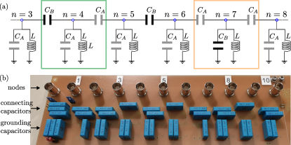
Figure 1: Fibonacci topoelectrical circuit. (a) The circuit diagram between nodes $n=3$ and $n=8$. Orange and green boxes indicate two different configurations of topoloelectrical circuit junctions. (b) A photograph of the corresponding segment of the circuit board. We see all elements of the circuit diagram of panel (a), except inductors that are located on the backside.

In the following, we describe an electrical circuit that realizes the Fibonacci chain. This circuit consists of $N=34$ nodes related by connecting wires and capacitors of distinct capacitances $C_{A}$ and $C_{B}$ that emulate the hoppings $t_{A},t_{B}$ of the tight-binding model and are thus arranged according to $\mathop{\rm sign}[\chi_{n}(\pi)]$. We show the circuit diagram inside the bulk of the system in Fig. 1(a), and in Fig. 1(b) the corresponding segment of a constructed circuit board. The orange and green boxes in Fig. 1(a) represent two possible local environments of bulk circuit nodes that differ by whether identical capacitances $(C_{A},C_{A})$ or distinct ones $(C_{A(B)},C_{B(A)})$ are used to relate a node $n$ to its neighbors. In the former (latter) case, for the grounding of node $n$ we use a capacitor of capacitance $\tilde{C}_{n}=C_{B}$ ($\tilde{C}_{n}=C_{A}$) that is connected in parallel to an inductor of inductance $L$, such that the relation $\tilde{C}_{n}+C_{n-1}+C_{n}=2C_{A}+C_{B}$ holds.

Each node is described by Kirchhoff’s law [30]

$$I_{n}=G_{n-1}(V_{n}-V_{n-1})+G_{n}(V_{n}-V_{n+1})+g_{n}V_{n},$$ (2)

where $G_{n}=2\pi jfC_{n}$ is the admittance between nodes $n$ and $n+1$, $f$ is the frequency, $C_{n}\in\{C_{A},C_{B}\}$ depending on $\mathop{\rm sign}[\chi_{n}(\pi)]$, and $j^{2}=-1$. The admittance $g_{n}$ between node $n$ and the ground equals $g_{n}=2\pi jf\tilde{C}_{n}+1/(2\pi jfL)$, where conductance $\tilde{C}_{n}\in\{C_{A},C_{B}\}$. By grouping all currents and voltages into vectors $\mathbf{I}$ and $\mathbf{V}$, we obtain the admittance matrix $Y(f)$

$$Y(f)=\tilde{g}(f)\mathbb{I}-2\pi jfH$$ (3)

in terms of which Kirchhoff’s rules are given by $\mathbf{I}(f)=Y(f)\mathbf{V}(f)$; here, $H$ is the Fibonacci Hamiltonian Eq. (1) with hoppings $t_{n}$ replaced by $C_{n}$ and $\tilde{g}(f)=2\pi jf(2C_{A}+C_{B})+1/(2\pi jfL)$.

To experimentally characterize the spectral properties of this circuit, we measure its response to the applied current $I(f)$. The voltage at node $b$ is related to an input current at node $a$ via the two-point impedance

$$Z_{a,b}(f)=\frac{V_{a}(f)-V_{b}(f)}{I_{a}(f)}=\sum_{n}\frac{|v_{n,a}-v_{n,b}|^{2}}{Y_{n}},$$ (4)

that can be calculated from the eigenvalues $Y_{n}(f)$ and eigenvectors $v_{n}(f)$ of the admittance matrix [30].

Next, we describe how $Z_{a,b}(f)$ can be used to reconstruct the Fibonacci chain spectrum. From Eq. (4), we see that $Z_{a,b}(f)$ has a pole at frequency $f_{n}$ every time $Y_{n}(f_{n})=0$. Using Eq. (3), we can relate the admittance matrix eigenvalues $Y_{n}$ to Hamiltonian eigenvalues $E_{n}$ as $Y_{n}(f)=\tilde{g}(f)-2\pi jfE_{n}$. Therefore, $Y_{n}(f_{n})=0\rightarrow E_{n}=\tilde{g}(f_{n})/2\pi jf_{n}$, resulting in

$$E_{n}=2C_{A}+C_{B}-\frac{1}{4\pi^{2}Lf^{2}_{n}};$$ (5)

we note in passing, that the energies are measured in units of capacitance. Due to the relation (5), reconstructing $E_{n}$ relies on identifying the resonance frequencies $f_{n}$ of the response function $Z_{a,b}(f)$. In the following, we describe how this can be done in practice.

Experimental setup and measurement analysis — For our experimental realization, we have used capacitors with nominal values of capacitances $C_{A}=50\,\rm nF$ and $C_{B}=100\,\rm nF$, and inductors with nominal inductances $L=10\,\rm\mu H$. The capacitors and inductors are high quality components bought from KEMET and WURTH Elektronik, respectively, that were pre-selected to vary less than $2\%$ from the corresponding nominal values of conductances and inductances. Importantly, these circuit elements have small but non-vanishing direct current resistances $R_{C}^{\text{dc}}\approx 25\,\rm m\Omega$ and $R_{L}^{\text{dc}}\approx 85\,\rm m\Omega$. In case of the inductors the resistance is frequency dependent and goes from $R_{L}^{\text{ac}}\approx 105\,\rm m\Omega$ (at $50\,\rm{kHz}$) to $R_{L}^{\text{ac}}\approx 308\,\rm m\Omega$ (at $250\,\rm{kHz}$). For more details, see the Supplemental Material (SM) [56].

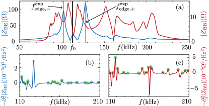
Figure 2: Absolute values of the measured impedances $|Z_{\rm BE}|$ and $|Z_{\rm BB}|$ [panel (a)] and their second derivatives $-\partial_{f}^{2}|Z_{\rm BE}|$ and $-\partial_{f}^{2}|Z_{\rm BB}|$ [panels (b) and (c)] as a function of frequency $f$. The green circles indicate the peaks of $-\partial_{f}^{2}|Z_{\rm BE}|$ and $-\partial_{f}^{2}|Z_{\rm BB}|$ in the frequency range $(f_{0},250\rm kHz)$, with $f_{0}=112.5\rm kHz$.

All measurements were performed with the lock-in amplifier SR865A manufactured by Stanford Research Systems [56]. We consider two configurations for the voltage probes; the “bulk-edge” (BE) configuration is realized by placing probes at nodes $a=1$ and $b=15$, while the “bulk-bulk” (BB) configuration has the probes at nodes $a=10$ and $b=24$. According to Eq. (4), the positions of the voltage probes determine the weights of the corresponding eigenstates in the impedance response. This results in a very different frequency dependence of the response functions $|{Z}_{\rm BE}|$ and $|{Z}_{\rm BB}|$ in range $f\in(50\rm\,kHz,250\,\rm kHz)$, see Fig. 2(a). To analyze these results, it is useful to define the frequency $f_{0}=112.5\,$kHz corresponding to $E=0$ as determined from Eq. (5) by setting $E_{n}=0$ and using experimental values for $C_{A},C_{B}$ and $L$.

Our first observation is that $|{Z}_{\rm BE}|$ and $|{Z}_{\rm BB}|$ have far fewer features for frequencies $f<f_{0}$ corresponding to energies $E<0$ than for $f>f_{0}$, where the positive part of the spectrum is located. This is a consequence of the nonlinear relationship between the eigenvalues $E_{n}$ and resonant frequencies $f_{n}$ in Eq. (5). This leads to the fact that the resonant frequencies of the negative eigenvalues are closer together than the ones corresponding to the positive eigenvalues. When this effect is combined with nonzero resistances $R_{C}^{\text{dc}},R_{L}^{\text{dc}}$ and $R_{L}^{ac}$ that broaden the-delta-peaks of the ideal response function into Lorentzians, the resonant peaks for frequencies $f<f_{0}$ are expected to be less visible than the ones for $f>f_{0}$ [56]. The second important feature of Fig. 2a is the observation that $|{Z}_{\rm BE}|$ has two very prominent peaks at frequencies (indicated by green lines) for which $|{Z}_{\rm BB}|$ does not show any prominent features. This suggests that these peaks are induced by topological edge modes [30]. From the corresponding frequencies $f^{\rm exp}_{\rm edge,-}\approx 101.7\,$kHz and $f^{\rm exp}_{\rm edge,+}\approx 127.5\,$kHz using Eq. (5), we obtain the energies $E^{\rm exp}_{\rm edge,-}=-44.9\,\rm nF$ and $E^{\rm exp}_{\rm edge,+}=44.2\,\rm nF$. Note that the theoretical value for energy of the edge states is $E_{\rm{edge},\pm}=\pm 43.7\rm nF$; the relative errors are $\delta^{r}=|(E^{\rm exp}_{\rm edge,-}-E_{\rm{edge},-})/E_{\rm{edge},-}|=2.75\%$ and $\delta^{r}=1.14\%$, respectively. Importantly, having $|E^{\rm exp}_{\rm edge,-}|\approx|E^{\rm exp}_{\rm edge,+}|\approx|E_{\rm edge,\pm}|$ is the experimental confirmation that the realized topoelectrical circuit has the chiral symmetry. We can use this symmetry to obtain an experimental value of the frequency $f_{0}^{\rm exp}=\frac{1}{2}(f^{\rm exp}_{\rm edge,-}+f^{\rm exp}_{\rm edge,+})=114.6\,$kHz with a relative error $\delta^{r}=1.87\%$ compared to $f_{0}$.

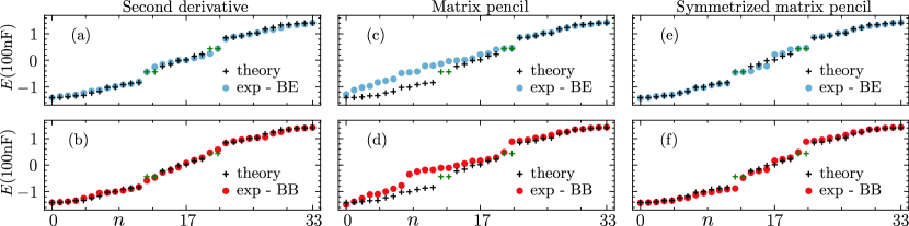
Figure 3: Comparison between the theoretical and experimental spectra obtained using different methods of recovery. Here, the green crosses indicate edge states. The eigenvalues in panels (a) and (b) are given by the maxima of $-\partial_{f}^{2}|Z_{\rm BE}|$ and $-\partial_{f}^{2}|Z_{\rm BB}|$, see green circles in Figs. 2(b) and (c). In panels (c) and (d), $34$ resonant frequencies are shown that were detected using the MP method. Panels (e) and (f) are obtained by mirroring the $17$ largest positive eigenvalues from panels (c) and (d) with respect to $E=0$.

To determine more eigenvalues, we focus on the second derivative of the response function because differentiation reduces the amplitude of broader peaks in the $Z_{a,b}(f)$ signal. This results in a better detection of resonances that have been previously obscured by a broader but stronger background [57]. In practice, calculating this derivative from the original data set is challenging because measurements always include some noise that manifests as random high-frequency and small amplitude deviations from the ideal signal. Since noise becomes more prominent with differentiation, we eliminate it from original data using a low-pass, $4$-th order Butterworth filter [58]. This filter has a maximally flat frequency response in the passband, thus not giving rise to any additional frequency dependence upon its application [58].

We employ two different strategies for extracting the Fibonacci chain spectrum. Our first approach is based on searching for the frequencies $f^{\rm exp}_{n}$ at which the function $-\partial_{f}^{2}|Z_{a,b}|$ (and consequently $|Z_{a,b}(f)|$) has peaks. To calculate $-\partial_{f}^{2}|Z_{a,b}|$, we employ the Butterworth filter with the cutoff frequency $f_{c}=0.01f_{\rm Nq}$ on $|Z_{a,b}(f)|$; here, $f_{\rm Nq}$ denotes the Nyquist frequency defined as half of the sampling frequency $f$. Due to aforementioned grouping effect of individual peaks in the lower frequency range, looking for $34$ most prominent peaks of $-\partial_{f}^{2}|Z_{a,b}|$ in the entire frequency range does not produce satisfying results. Because of the chiral symmetry, we can instead focus on the frequency range $(f_{0},250\rm kHz)$ that corresponds to the positive part of the spectrum consisting of $17$ eigenvalues. Using the SCIPY Python library [59], we find all the peaks of $-\partial_{f}^{2}|Z_{\rm BE}|$ and $-\partial_{f}^{2}|Z_{\rm BB}|$ in this frequency range and choose the $17$ most prominent ones for both curves. These peaks are indicated with green circles in Figs. 2(b) and (c) for $-\partial_{f}^{2}|Z_{\rm BE}|$ and $-\partial_{f}^{2}|Z_{\rm BB}|$, respectively.

The corresponding spectra are constructed from pairs $(-E^{\rm exp}_{n},E^{\exp}_{n})$, with $E^{\exp}_{n}$ obtained from $f^{\rm exp}_{n}$ using Eq. (5). We plot these spectra in Figs. 3(a) and (b) for the BE and BB voltage probe configurations, respectively, along with the theoretical eigenvalues $E_{n}$. We observe that both voltage probes are successful in detecting the edges of the upper band (and consequently the lower band), along with its inner sub-bands. The BE probe captures accurately the energies of two pairs of edge states but it detects a single resonance per pair. This behavior is also present for an ideal circuit, and originates from the energy degeneracy of two edge modes. On the other side, the BB probe detects two resonances inside the topological gap but is less accurate in measuring the energies of edge states. In total, for the BE probe the mean absolute error $\delta^{\rm avg}=\sum_{n=1}^{N}|E_{n}-E_{n}^{\rm exp}|/N$ equals $\delta^{\rm avg}_{\rm BE}=4.87\,\rm nF$ while the median error is $\delta_{\rm BE}^{m}=3.81\,\rm nF$. For the BB probe, we find $\delta^{\rm avg}_{\rm BB}=4.17\,\rm nF$ and $\delta_{\rm BB}^{m}=3.18\,\rm nF$.

As these errors are small compared to the total energy range, we conclude that searching for peaks of $-\partial_{f}^{2}|Z_{a,b}|$ is a fruitful strategy to recover the full spectrum. However, this approach focuses only on the amplitude of the frequency dependent response function, and thus misses possible information hidden in the corresponding phase component. To rectify this, we employ our second approach that is based on fitting the full signal $-\partial_{f}^{2}Z_{a.b}$ to the linear combination of Lorentzians. To eliminate noise from the data, we use the Butterworth filter separately on $\Re[Z_{a,b}(f)]$ and $\Im[Z_{a,b}(f)]$ before calculating their second derivatives with respect to frequency and combining them to obtain $-\partial_{f}^{2}Z_{a,b}$. We use frequency cutoffs $f_{c}=0.03f_{\rm Nq}$ $(f_{c}=0.01f_{\rm Nq})$ for the BE (BB) configuration of voltage probes. The resulting signal $-\partial_{f}^{2}Z_{a,b}$ is Fourier transformed into the time domain signal $Z^{(2)}_{a,b}(t)=\mathcal{F}[-\partial_{f}^{2}Z_{a,b}]$ that is fitted to a sum of $N$ damped exponentials as

$$Z^{(2)}_{a,b}(t)=\sum_{n=1}^{N}A^{\rm exp}_{n}e^{j\phi^{\rm exp}_{n}}e^{(\alpha^{\rm exp}_{n}+2\pi jf^{\rm exp}_{n})t},$$ (6)

where $A^{\rm exp}_{n},\phi^{\rm exp}_{n},\alpha^{\rm exp}_{n}$ and $f^{\rm exp}_{n}$ are the amplitudes, phases, damping factors and frequencies of the sinusoids, respectively. Assuming $t=mT$ where $m=0,...,N-1$ and $T$ is the sampling period, the exponential factor becomes $e^{(\alpha^{\rm exp}_{n}+2\pi jf^{\rm exp}_{n})mT}=z_{n}^{m}$, where $z_{n}=e^{(\alpha^{\rm exp}_{n}+2\pi jf^{\rm exp}_{n})T}$. The poles $z_{n}$ are found by solving a generalized eigenvalue equation using a matrix pencil (MP) operator that is constructed from the values $Z^{(2)}_{a,b}(t)$ [60, 61, 62], see also the SM [56]. As there are $34$ eigenvalues in theory, we look for $34$ poles in our calculation.

The resulting spectrum, obtained using Eq. (5), is shown in Figs. 3(c) and (d) for both voltage probe configurations. While this approach can reconstruct the entire spectrum, we see that for both configurations it works better for positive eigenvalues, i.e., for frequencies $f>f_{0}$. In general, the accuracy of the MP method declines as the energy is reduced which can be expected due to the aforementioned grouping effect of resonances. Moreover, for both probes, the method finds $15$ ($19$) poles corresponding to negative (positive) energies. The additional positive poles arise at $E\sim 1\rm nF$ that is very close to $E=0$ in comparison with the energy scale of the chain. In case of the BE probe where the edge modes dominate the response of the circuit, the MP method overestimates the number of edge modes in the upper topological gap but captures their energies well. For the BB probe, the method finds a single mode for a pair of edge modes with $E>0$, and attributes the missing edge mode resonance to the upper band. In total, we find $\delta^{\rm avg}_{\rm BE}=21.67\,\rm nF,\delta^{m}_{\rm BE}=14.09\,\rm nF$, and $\delta^{\rm avg}_{\rm BB}=19.83\,\rm nF,\delta^{m}_{\rm BB}=11.54\,\rm nF$. Such large values of errors reflect the fact that the MP method misses to capture the negative eigenvalues accurately.

The results of the MP-method can be improved by utilizing the spectral symmetry constraint, i.e., by constructing spectra from pairs $(-E^{\rm exp}_{n},E^{\rm exp}_{n})$, where $E^{\rm exp}_{n}>0$ are $17$ largest positive eigenvalues from Figs. 3(c) and (d). Results are shown in Figs. 3(e) and (f) for BE and BB configurations, respectively. This combined approach reduces the errors of measurements to $\delta^{\rm avg}_{\rm BE}=4.24\,\rm nF$, $\delta^{m}_{\rm BE}=2.22\,\rm nF$ for the BE probe and $\delta^{\rm avg}_{\rm BB}=7.68\,\rm nF$, $\delta^{m}_{\rm BB}=5.22\,\rm nF$ for the BB probe. Therefore, combining the MP method with the spectral symmetry constraint works the best for the BE probe, while searching for the peaks of $-\partial_{f}^{2}|Z_{a,b}|$ yields better results for the BB probe.

For both probes, our best results have $\delta_{a,b}^{\rm avg}\approx\delta_{E}/2$, where $\delta_{E}=8.55\rm nF$ is a theoretical average energy spacing. These results could be improved by reducing the noise in the measurement and the resistances of circuit elements. Contrary to the present study that separately measured $V_{a}(f),V_{b}(f),I_{a}(f)$ thus increasing the chance of random events, employing additional lock-in amplifiers would allow for a simultaneous measurement of all three quantities and thus reduce the noise. Reducing resistances of circuit elements, on the other hand, is not straightforward: for example, lowering $R_{L}^{\text{ac}}(100\rm kHz)$ generally requires reducing the inductance $L$ of inductors, resulting in a larger frequency range needed to determine all the eigenvalues which leads to an increased of $R_{L}^{\text{ac}}$. As a result, the inductors will produce additional heating which washes out features due to the increased noise. An interesting idea for future research is to investigate whether superconducting elements with significantly smaller resistances can improve the accuracy of our results.

Conclusion — In this work, we have shown how the response function of an electrical circuit can be used to recover the full spectrum of an underlying condensed matter system simulated by this circuit. We have constructed, for the first time, the Fibonacci topoelectrical chain that has a fractal spectrum due to its quasicrystalline nature. We have demonstrated that the spectrum can be recovered from a single measurement using two distinct methods of data analysis. We have corroborated our findings by changing the positions of the voltage probes as well as the boundary conditions of the Fibonacci topoelectrical circuit [56]. In conclusion, our work promotes topoelectrical circuits as an ideal meta-material platform for studying spectral properties of (quasi)crystalline systems.

Acknowledgements — We thank Ulrike Nitzsche for technical assistance. This work was supported by the Deutsche Forschungsgemeinschaft (DFG, German Research Foundation) under Germany’s Excellence Strategy through the Würzburg-Dresden Cluster of Excellence on Complexity and Topology in Quantum Matter – ct.qmat (EXC 2147, project-id 390858490) and under Germany’s Excellence Strategy – Cluster of Excellence Matter and Light for Quantum Computing (ML4Q) EXC 2004/1 – 390534769. S. F. acknowledges financial support from the European Union Horizon 2020 research and innovation program under grant agreement No. 829044 (SCHINES).

Competing Interests Statement — The authors declare no competing interests.

References

- Haldane and Raghu [2008] F. D. M. Haldane and S. Raghu, Possible realization of directional optical waveguides in photonic crystals with broken time-reversal symmetry, Phys. Rev. Lett. 100, 013904 (2008).
- von Klitzing et al. [1980] K. von Klitzing, G. Dorda, and M. Pepper, New method for high-accuracy determination of the fine-structure constant based on quantized Hall resistance, Phys. Rev. Lett. 45, 494 (1980).
- Lu et al. [2014] L. Lu, J. D. Joannopoulos, and M. Soljačić, Topological photonics, Nature Photon. 8, 821 (2014).
- Zeuner et al. [2015] J. M. Zeuner, M. C. Rechtsman, Y. Plotnik, Y. Lumer, S. Nolte, M. S. Rudner, M. Segev, and A. Szameit, Observation of a topological transition in the bulk of a non-Hermitian system, Phys. Rev. Lett. 115, 040402 (2015).
- Weimann et al. [2017] S. Weimann, M. Kremer, Y. Plotnik, Y. Lumer, S. Nolte, K. G. Makris, M. Segev, M. C. Rechtsman, and A. Szameit, Topologically protected bound states in photonic parity–time-symmetric crystals, Nature Mater. 16, 433 (2017).
- Noh et al. [2018] J. Noh, W. A. Benalcazar, S. Huang, M. J. Collins, K. P. Chen, T. L. Hughes, and M. C. Rechtsman, Topological protection of photonic mid-gap defect modes, Nature Photon. 12, 408 (2018).
- Saei Ghareh Naz et al. [2018] E. Saei Ghareh Naz, I. C. Fulga, L. Ma, O. G. Schmidt, and J. van den Brink, Topological phase transition in a stretchable photonic crystal, Phys. Rev. A 98, 033830 (2018).
- Chen et al. [2019] X.-D. Chen, W.-M. Deng, F.-L. Shi, F.-L. Zhao, M. Chen, and J.-W. Dong, Direct observation of corner states in second-order topological photonic crystal slabs, Phys. Rev. Lett. 122, 233902 (2019).
- Mittal et al. [2019] S. Mittal, V. V. Orre, G. Zhu, M. A. Gorlach, A. Poddubny, and M. Hafezi, Photonic quadrupole topological phases, Nature Photon. 13, 692 (2019).
- El Hassan et al. [2019] A. El Hassan, F. K. Kunst, A. Moritz, G. Andler, E. J. Bergholtz, and M. Bourennane, Corner states of light in photonic waveguides, Nature Photon. 13, 697 (2019).
- Torrent and Sánchez-Dehesa [2012] D. Torrent and J. Sánchez-Dehesa, Acoustic analogue of graphene: Observation of Dirac cones in acoustic surface waves, Phys. Rev. Lett. 108, 174301 (2012).
- Yang et al. [2015] Z. Yang, F. Gao, X. Shi, X. Lin, Z. Gao, Y. Chong, and B. Zhang, Topological acoustics, Phys. Rev. Lett. 114, 114301 (2015).
- Fan et al. [2016] L. Fan, W.-w. Yu, S.-y. Zhang, H. Zhang, and J. Ding, Zak phases and band properties in acoustic metamaterials with negative modulus or negative density, Phys. Rev. B 94, 174307 (2016).
- Xue et al. [2019] H. Xue, Y. Yang, F. Gao, Y. Chong, and B. Zhang, Acoustic higher-order topological insulator on a kagome lattice, Nature Mater. 18, 108 (2019).
- Ni et al. [2019a] X. Ni, M. Weiner, A. Alù, and A. B. Khanikaev, Observation of higher-order topological acoustic states protected by generalized chiral symmetry, Nature Mater. 18, 113 (2019a).
- Apigo et al. [2019] D. J. Apigo, W. Cheng, K. F. Dobiszewski, E. Prodan, and C. Prodan, Observation of topological edge modes in a quasiperiodic acoustic waveguide, Phys. Rev. Lett. 122, 095501 (2019).
- Ni et al. [2019b] X. Ni, K. Chen, M. Weiner, D. J. Apigo, C. Prodan, A. Alù, E. Prodan, and A. B. Khanikaev, Observation of Hofstadter butterfly and topological edge states in reconfigurable quasi-periodic acoustic crystals, Commun. Phys. 2, 55 (2019b).
- Chen et al. [2021] Z.-G. Chen, W. Tang, R.-Y. Zhang, Z. Chen, and G. Ma, Landau-Zener transition in the dynamic transfer of acoustic topological states, Phys. Rev. Lett. 126, 054301 (2021).
- Süsstrunk and Huber [2015] R. Süsstrunk and S. D. Huber, Observation of phononic helical edge states in a mechanical topological insulator, Science 349, 47 (2015).
- Bertoldi et al. [2017] K. Bertoldi, V. Vitelli, J. Christensen, and M. van Hecke, Flexible mechanical metamaterials, Nat. Rev. Mater. 2, 17066 (2017).
- Serra-Garcia et al. [2018] M. Serra-Garcia, V. Peri, R. Süsstrunk, O. R. Bilal, T. Larsen, L. G. Villanueva, and S. D. Huber, Observation of a phononic quadrupole topological insulator, Nature 555, 342 (2018).
- Bellec et al. [2013] M. Bellec, U. Kuhl, G. Montambaux, and F. Mortessagne, Topological transition of dirac points in a microwave experiment, Phys. Rev. Lett. 110, 033902 (2013).
- Hu et al. [2015] W. Hu, J. C. Pillay, K. Wu, M. Pasek, P. P. Shum, and Y. D. Chong, Measurement of a topological edge invariant in a microwave network, Phys. Rev. X 5, 011012 (2015).
- Anderson et al. [2016] B. M. Anderson, R. Ma, C. Owens, D. I. Schuster, and J. Simon, Engineering topological many-body materials in microwave cavity arrays, Phys. Rev. X 6, 041043 (2016).
- Peterson et al. [2018] C. W. Peterson, W. A. Benalcazar, T. L. Hughes, and G. Bahl, A quantized microwave quadrupole insulator with topologically protected corner states, Nature 555, 346 (2018).
- Yu et al. [2020] Y. Yu, W. Song, C. Chen, T. Chen, H. Ye, X. Shen, Q. Cheng, and T. Li, Phase transition of non-Hermitian topological edge states in microwave regime, Appl. Phys. Lett. 116, 211104 (2020).
- Ma and Anlage [2020] S. Ma and S. M. Anlage, Microwave applications of photonic topological insulators, Appl. Phys. Lett. 116, 250502 (2020).
- Ningyuan et al. [2015] J. Ningyuan, C. Owens, A. Sommer, D. Schuster, and J. Simon, Time- and site-resolved dynamics in a topological circuit, Phys. Rev. X 5, 021031 (2015).
- Albert et al. [2015] V. V. Albert, L. I. Glazman, and L. Jiang, Topological properties of linear circuit lattices, Phys. Rev. Lett. 114, 173902 (2015).
- Lee et al. [2018] C. H. Lee, S. Imhof, C. Berger, F. Bayer, J. Brehm, L. W. Molenkamp, T. Kiessling, and R. Thomale, Topolectrical circuits, Commun. Phys. 1, 39 (2018).
- Goren et al. [2018] T. Goren, K. Plekhanov, F. Appas, and K. Le Hur, Topological Zak phase in strongly coupled LC circuits, Phys. Rev. B 97, 041106 (2018).
- Li et al. [2018] Y. Li, Y. Sun, W. Zhu, Z. Guo, J. Jiang, T. Kariyado, H. Chen, and X. Hu, Topological LC-circuits based on microstrips and observation of electromagnetic modes with orbital angular momentum, Nat. Commun. 9, 4598 (2018).
- Hofmann et al. [2019] T. Hofmann, T. Helbig, C. H. Lee, M. Greiter, and R. Thomale, Chiral voltage propagation and calibration in a topolectrical Chern circuit, Phys. Rev. Lett. 122, 247702 (2019).
- Haenel et al. [2019] R. Haenel, T. Branch, and M. Franz, Chern insulators for electromagnetic waves in electrical circuit networks, Phys. Rev. B 99, 235110 (2019).
- Zhu et al. [2019] W. Zhu, Y. Long, H. Chen, and J. Ren, Quantum valley Hall effects and spin-valley locking in topological Kane-Mele circuit networks, Phys. Rev. B 99, 115410 (2019).
- Helbig et al. [2020] T. Helbig, T. Hofmann, S. Imhof, M. Abdelghany, T. Kiessling, L. W. Molenkamp, C. H. Lee, A. Szameit, M. Greiter, and R. Thomale, Generalized bulk-boundary correspondence in non-Hermitian topolectrical circuits, Nature Phys. 16, 747 (2020).
- Hofmann et al. [2020] T. Hofmann, T. Helbig, F. Schindler, N. Salgo, M. Brzezińska, M. Greiter, T. Kiessling, D. Wolf, A. Vollhardt, A. Kabaši, C. H. Lee, A. Bilušić, R. Thomale, and T. Neupert, Reciprocal skin effect and its realization in a topolectrical circuit, Phys. Rev. Res. 2, 023265 (2020).
- Wang et al. [2020] Y. Wang, H. M. Price, B. Zhang, and Y. D. Chong, Circuit implementation of a four-dimensional topological insulator, Nat. Commun. 11, 2356 (2020).
- Rafi-Ul-Islam et al. [2020] S. M. Rafi-Ul-Islam, Z. Bin Siu, and M. B. A. Jalil, Topoelectrical circuit realization of a Weyl semimetal heterojunction, Commun. Phys. 3, 72 (2020).
- Dong et al. [2021] J. Dong, V. Juričić, and B. Roy, Topolectric circuits: Theory and construction, Phys. Rev. Res. 3, 023056 (2021).
- Kotwal et al. [2021] T. Kotwal, F. Moseley, A. Stegmaier, S. Imhof, H. Brand, T. Kießling, R. Thomale, H. Ronellenfitsch, and J. Dunkel, Active topolectrical circuits, PNAS 118, e2106411118 (2021).
- Yang et al. [2023] H. Yang, L. Song, Y. Cao, and P. Yan, Realization of Wilson fermions in topolectrical circuits, Commun. Phys. 6, 211 (2023).
- Zheng et al. [2022] X. Zheng, T. Chen, and X. Zhang, Topolectrical circuit realization of quadrupolar surface semimetals, Phys. Rev. B 106, 035308 (2022).
- Zhang et al. [2023] H. Zhang, T. Chen, L. Li, C. H. Lee, and X. Zhang, Electrical circuit realization of topological switching for the non-Hermitian skin effect, Phys. Rev. B 107, 085426 (2023).
- Imhof et al. [2018] S. Imhof, C. Berger, F. Bayer, J. Brehm, L. W. Molenkamp, T. Kiessling, F. Schindler, C. H. Lee, M. Greiter, T. Neupert, and R. Thomale, Topolectrical-circuit realization of topological corner modes, Nature Phys. 14, 925 (2018).
- Stegmaier et al. [2021] A. Stegmaier, S. Imhof, T. Helbig, T. Hofmann, C. H. Lee, M. Kremer, A. Fritzsche, T. Feichtner, S. Klembt, S. Höfling, I. Boettcher, I. C. Fulga, L. Ma, O. G. Schmidt, M. Greiter, T. Kiessling, A. Szameit, and R. Thomale, Topological defect engineering and symmetry in non-Hermitian electrical circuits, Phys. Rev. Lett. 126, 215302 (2021).
- Lenz and Stollmann [2003] D. Lenz and P. Stollmann, Aperiodic order and quasicrystals: Spectral properties, Ann. Henri Poincaré 4, 933 (2003).
- Pikovsky et al. [1995] A. S. Pikovsky, M. A. Zaks, U. Feudel, and J. Kurths, Singular continuous spectra in dissipative dynamics, Phys. Rev. E 52, 285 (1995).
- Jagannathan [2021] A. Jagannathan, The Fibonacci quasicrystal: Case study of hidden dimensions and multifractality, Rev. Mod. Phys. 93, 045001 (2021).
- Tanese et al. [2014] D. Tanese, E. Gurevich, F. Baboux, T. Jacqmin, A. Lemaître, E. Galopin, I. Sagnes, A. Amo, J. Bloch, and E. Akkermans, Fractal energy spectrum of a polariton gas in a Fibonacci quasiperiodic potential, Phys. Rev. Lett. 112, 146404 (2014).
- Kraus et al. [2012] Y. E. Kraus, Y. Lahini, Z. Ringel, M. Verbin, and O. Zilberberg, Topological states and adiabatic pumping in quasicrystals, Phys. Rev. Lett. 109, 106402 (2012).
- Verbin et al. [2013] M. Verbin, O. Zilberberg, Y. E. Kraus, Y. Lahini, and Y. Silberberg, Observation of topological phase transitions in photonic quasicrystals, Phys. Rev. Lett. 110, 076403 (2013).
- Stegmaier et al. [2023] A. Stegmaier, H. Brand, S. Imhof, A. Fritzsche, T. Helbig, T. Hofmann, I. Boettcher, M. Greiter, C. H. Lee, G. Bahl, A. Szameit, T. Kießling, R. Thomale, and L. K. Upreti, Realizing efficient topological temporal pumping in electrical circuits, Preprint at https://arxiv.org/abs/2306.15434 (2023).
- Zou et al. [2023] D. Zou, T. Chen, H. Meng, Y. S. Ang, X. Zhang, and C. H. Lee, Experimental observation of exceptional bound states in a classical circuit network, Preprint at https://arxiv.org/abs/2308.01970 (2023).
- Sütő [1989] A. Sütő, Singular continuous spectrum on a Cantor set of zero Lebesgue measure for the Fibonacci Hamiltonian, J. Stat. Phys. 56, 525 (1989).
- [56] In the Supplemental Material, we show details of the experimental realization before discussing how realistic capacitors and inductors affect the two point impedance. We proceed with discussing the matrix pencil method, before showing reconstructed spectra for the system under periodic boundary conditions. .
- O’Haver [2023] T. O’Haver, A Pragmatic Introduction to Signal Processing 2023: with applications in scientific measurement, McGraw-Hill series in electrical engineering (Independently Published, 2023).
- Butterworth [1930] S. Butterworth, On the Theory of Filter Amplifiers, Experimental Wireless & the Wireless Engineer 7, 536 (1930).
- Franca et al. [2023] S. Franca, T. Seidemann, F. Hassler, J. van den Brink, and I. C. Fulga, Two-point spectroscopy of Fibonacci topoelectrical circuits, Zenodo 10.5281/zenodo.8386622 (2023).
- Hua and Sarkar [1990] Y. Hua and T. Sarkar, Matrix pencil method for estimating parameters of exponentially damped/undamped sinusoids in noise, IEEE Transactions on Acoustics, Speech, and Signal Processing 38, 814 (1990).
- Vanhamme et al. [2001] L. Vanhamme, T. Sundin, P. V. Hecke, and S. V. Huffel, MR spectroscopy quantitation: a review of time-domain methods, NMR in Biomedicine 14, 233 (2001).
- Zieliński and Duda [2011] T. P. Zieliński and K. Duda, Frequency and damping estimation methods - an overview, Metrology and Measurement Systems 18, 505 (2011).