2-Cats: 2D Copula Approximating Transforms

Abstract

Copulas are powerful statistical tools for capturing dependencies across multiple data dimensions. Applying Copulas involves estimating independent marginals, a straightforward task, followed by the much more challenging task of determining a single copulating function, $C$, that links these marginals. For bivariate data, a copula takes the form of a two-increasing function $C:(u,v)\in\mathbb{I}^{2}\rightarrow\mathbb{I}$, where $\mathbb{I}=[0,1]$. In this paper, we propose 2-Cats, a Neural Network (NN) model that learns two-dimensional Copulas while preserving their key properties, without relying on specific Copula families (e.g., Archimedean). Furthermore, we introduce a training strategy inspired by the literature on Physics-Informed Neural Networks and Sobolev Training. Our proposed method exhibits superior performance compared to the state-of-the-art across various datasets while maintaining the fundamental mathematical properties of a Copula.

1 Introduction

Modeling univariate data is relatively straightforward for several reasons. Firstly, there exists a wide range of probability distributions suitable for different types of data, including Gaussian, Beta, Log-Normal, Gamma, and Poisson. This set is expanded by mixture models that use the basic distributions as components and can model multimodality and other behavior. Secondly, visual tools such as histograms or Kernel Density Estimators (KDE) provide valuable assistance in selecting the appropriate distribution. Lastly, univariate models typically involve few parameters and may even have exact solutions, simplifying the modeling process.

However, the process becomes more challenging when modeling multivariate data and obtaining a joint probability distribution. Firstly, only a few classes of multivariate probability distributions are available, with the primary exceptions being the multivariate Gaussian, Elliptical, and Dirichlet distributions. Secondly, simultaneously identifying the dependencies among multiple variables is not easy. Distinguishing direct dependencies from conditional independence based solely on empirical data is a highly complex task.

In 1959, Abe Sklar formalized the idea of Copulas [Sklar, 1959, 1996]. This statistical tool allows us to model a multivariate random variable of dimension $d$ by learning its cumulative multivariate distribution function (CDF) using $d$ independent marginal CDFs and a single additional Copulating function $C$. A bivariate example may separately identify one marginal as a Log-Normal distribution and the other as a Beta distribution. Subsequently, the Copula model links these two marginal distributions.

However, the Copula approach to modeling multivariate data faced a significant limitation until recently. Our model choices were confined to only a handful of closed forms for the $C$ Copulas, such as the Gaussian, Frank, or Clayton Copulas [Czado and Nagler, 2022, Größer and Okhrin, 2022]. Unfortunately, this approach using closed-form Copula models proved inadequate for accurately capturing the complex dependencies in real data. The limited parameterization of these Copulas prevented them from fully representing the intricate relationships between variables.

This situation has changed recently. Neural Networks (NNs) are well-known for their universal ability to approximate any function. Consequently, researchers have started exploring NNs as alternatives to closed forms for $C$ [Chilinski and Silva, 2020, Hirt et al., 2019, Tagasovska et al., 2023, Janke et al., 2021, Ling et al., 2020, Ng et al., 2021]. However, a limitation of several NN models (not only for Copulas) is that they neglect the importance of maintaining the fundamental mathematical properties of their domain of study.

For Copulas, only three properties define $C$ [Nelsen, 2006]: P1: $C:(u,v)\in\mathbb{I}^{2}\mapsto\mathbb{I}$, where $\mathbb{I}=[0,1]$.
P2: $C$ is grounded. That is, $C(0,v)=0$, $C(v,0)=0$. Moreover, $C(1,v)=v$ and $C(u,1)=u$.
P3: For any $0\leq u_{1}<u_{2}\leq 1$ and $0\leq v_{1}<v_{2}\leq 1$, we have that the volume of $C$ is: $V_{C}(u_{1},u_{2},v_{1},v_{2})\equiv C(u_{2},v_{2})-C(u_{2},v_{1})-C(u_{1},v_{2})+C(u_{1},y_{1})\geq 0$.

Our model, 2-Cats, is a NN approach that meets such properties. The formal proofs are in Section 3.2

Other properties of a Copula arise as a consequence of the above three. For instance, given a Copula function $C$, its second partial derivative $c(u,v)=\frac{\partial^{2}C(u,v)}{\partial u\partial v}\geq 0$ is the probability density function (PDF) associated with $C$ (i.e., $c:\mathbb{I}^{2}\mapsto\mathbb{R}^{+}$ with $\iint c(u,v)\;du\;dv=1$) [Nelsen, 2006].

In this paper, we propose 2-Cats (2D Copula Approximating Transforms). To understand our approach, let $H_{\theta}(u,v)$ represent our copula model (or Hypothesis). Let $G:\mathbb{R}^{2}\mapsto\mathbb{I}$ be any bivariate CDF with $\mathbb{R}^{2}$ as support. Examples are the bivariate Normal or bivariate Logistic. We connect $H_{\bm{\theta}}$ with $G$ as follows:

$$H_{\bm{\theta}}(u,v) =G\Big{(}z\big{(}t_{v}(u)\big{)},z(t_{u}(v)\big{)}\Big{)};\,\,z(x)=\log(\frac{x}{1-x});$$

$$t_{v}(u) =\frac{\int_{0}^{u}m_{\bm{\theta}}(x,v)\,dx}{\int_{0}^{1}m_{\bm{\theta}}(x^{\prime},v)\,dx^{\prime}};\,\,t_{u}(v)=\frac{\int_{0}^{v}m_{\bm{\theta}}(u,y)\,dy}{\int_{0}^{1}m_{\bm{\theta}}(u,y^{\prime})\,dy^{\prime}};$$

Here, $m_{\bm{\theta}}(u,v)$ is any NN that outputs a positive number and $z(x)$ is the Logit function that is both monotonic and maps $[0,1]$ to $[-\infty,\infty]$, i.e., $z:\mathbb{I}\mapsto\mathbb{R}$. Here, the function $t_{v}(u)$ is monotonically increasing concerning $u$ because of the positive NN output; similarly, $t_{u}(v)$ is monotonic on $v$.

The monotonic properties of all transformations ensure that our output $H_{\bm{\theta}}(u,v)$ is monotonic for both $u$ and $v$. Let $z_{u}=z(t_{v}(u))$ and $z_{v}=z(t_{u}(v))$ to simplify notation and $(U,V)$ a random vector with distribution function $H_{\bm{\theta}}(u,v)$. Then, the probability transform below is valid [Casella and Berger, 2001, section 4.3]:

$$H_{\bm{\theta}}(u,v) =\Pr\big{[}U\leq u,V\leq v\big{]}$$

$$=\Pr\big{[}t^{-1}_{v}(U)\leq t^{-1}_{v}(u),t^{-1}_{v}(V)\leq t^{-1}_{v}(v)\big{]};$$

$$=\Pr\big{[}Z_{u}\leq z_{u},Z_{v}\leq z_{v}\big{]}$$

As we prove in Section 3.2, this guarantees that $H_{\bm{\theta}}(u,v)$ is a Copula and meets the P1-P3 properties.

There have been several recent NN Copula/CDF-based models [Chilinski and Silva, 2020, Ling et al., 2020, Ng et al., 2021] and non-NN models Nagler et al. [2017], Bakam and Pommeret [2023], Mukhopadhyay and Parzen [2020]. We compare our 2-Cats model with these alternatives and our results in Section 5 show that the 2-Cats performance (in negative log-likelihood) is better or statistically tied to the results from the state-of-the-art.

A second contribution of our work is that 2-Cats models are trained similarly to Physics Informed Neural Networks (PINNs) [Karniadakis et al., 2021, Lu et al., 2021]. We employ Sobolev training [Czarnecki et al., 2017] to minimize losses concerning an objective function and its derivatives. Ours is the first NN-based Copula work to do so and it bridges two research areas.

In summary, our contributions can be outlined as follows:

• We introduce the 2-Cats model, a novel neural network-based Copula that not only satisfies all the essential requirements of a Copula (refer to Section 3.2), but also demonstrates empirical accuracy as an effective approximator for various 2-D Copulas.

• Beyond meeting the fundamental properties of a Copula, our model enables the estimation of the Jacobian and Hessian of the Copula through symbolic differentiation. This capability allows us to assess several crucial aspects: the likelihood of the Copula (or the pseudo-likelihood of the data, defined as the second derivative); the conditional empirical distributions of the Copula (first derivative); the inverse of the previous function, inverse of the conditional, useful for sampling; and, the cumulative function (the Copula itself).

• We are the first to apply Sobolev training [Czarnecki et al., 2017] in NN-based Copula methodologies. Our approach involves the introduction of a simple empirical estimator for the first derivative of a Copula, seamlessly integrating it into our training framework.

2 Related Work

After being introduced by Sklar [Sklar, 1959, 1996], Copulas have emerged as valuable tools across various domains [Größer and Okhrin, 2022, Nelsen, 2006], including engineering [Salvadori and De Michele, 2004], geosciences [Modiri et al., 2020, Yang et al., 2019], and finance [Cherubini et al., 2004, Salvadori and De Michele, 2004]. Recently, Copulas have gained attention from the machine learning (ML) community, particularly with the advent of Deep Learning methods for Copula estimation and their utilization in generative models [Chilinski and Silva, 2020, Hirt et al., 2019, Tagasovska et al., 2023, Ling et al., 2020, Janke et al., 2021, Ng et al., 2021].

Our proposed approach aligns closely with the emerging literature in this domain but makes significant advancements on two fronts. This paper primarily focuses on developing an NN-based Copula model that adheres to the fundamental properties of a Copula. Two methods sharing similar objectives are discussed in [Ling et al., 2020, Ng et al., 2021] and [Chilinski and Silva, 2020]. However, our approach diverges from these prior works by not confining our method to Archimedean Copulas, as seen in [Ling et al., 2020] and [Ng et al., 2021].

As Chilinski and Silva [Chilinski and Silva, 2020], we begin by estimating densities through CDF estimations followed by automatic differentiation to acquire densities. However, our primary differentiation lies in our emphasis on fulfilling the requisite properties of a copula, an aspect not prioritized by the authors of that study.

To assess the effectiveness of our approach, we conduct comparative analyses against previous proposals, including the method presented by Janke et al. [Janke et al., 2021], proposed as a generative model. Furthermore, 2-Cats does not presume a fixed density function for copula estimation; instead, it is guided by the neural network (NN). Hence, our work shares similarities with non-parametric copula estimators used as baselinesNagler et al. [2017], Mukhopadhyay and Parzen [2020], Bakam and Pommeret [2023]. Ultimately, all these methods function as baseline approaches against which we evaluate and demonstrate the superiority of our proposed approach.

For training our models, we utilize Sobolev training as a regularizer. Sobolev training is tailored to estimate neural networks (NNs) by incorporating losses that not only address errors toward the primary objective but also consider errors toward their derivatives. This approach ensures a more comprehensive and accurate training of the NNs. A similar concept is explored in Physics Informed Neural Networks (PINNs) [Karniadakis et al., 2021, Kobyzev et al., 2020], where NNs incorporate derivative information from physical models. This derivative-aware training enables PINNs to better capture complex physics-related relationships.

In summary, our objective is to develop an NN-based Copula model that respects the mathematical properties of Copulas and benefits from considering derivative information. Consequently, although our focus is on 2D Copulas, the Pair Copula Decomposition (PCC) [Aas et al., 2009, Czado, 2010] that requires derivative information and is used to model $d$-dimensional data is valid for our models [Czado and Nagler, 2022]. Due to space constraints, we leave the evaluation of such a decomposition for future work.

Our work also aligns with the literature on monotonic networks [Sill, 1997, Daniels and Velikova, 2010, Wehenkel and Louppe, 2019]. The concept of using integral transforms to build monotonic models was introduced by Wehenkel and Louppe [2019]. This idea is currently evolving in the form of Integral Networks [Kortvelesy, 2023, Liu, 2023].

3 Properties and Proofs

We now revisit the discussion on the 2-Cats model as introduced in Section 1. Specifically, we will elaborate on the model’s implementation and rigorously establish the validity of 2-Cats as a copula.

3.1 Implementation Details

One of the building blocks of 2-Cats is the NN $m_{\bm{\theta}}(u,v)$. In particular, we require that this NN outputs only positive numbers and that its integral captures a monotonic function. We achieve this by employing Exponential Linear Units (ELU) plus one activation (ELU+1) in every layer as is the Unconstrained Monotonic Network defined by  Wehenkel and Louppe [2019].

Let us consider the computation details of $t_{v}(u)$, with the understanding that the process for $t_{u}(v)$ is analogous. In our implementation, we adopt Cumulative Trapezoid integration. Initially, we divide the range $[0,1]$ into $200$ equally spaced intervals. When computing $t_{v}(u)$, the value of $u$ is inserted into this interval while preserving the order. Subsequently, the $m_{\bm{\theta}}(x,v)$ NN is evaluated for the $201$ corresponding values of parameter $x$. Trapezoidal integration is then applied to calculate the integral value at $u$ (for the numerator) and $1$ (for the denominator). Finally, when $u=0$, it follows that $t_{v}(0)=0$.

To compute the Jacobian and Hessian of $H_{\bm{\theta}}$, as is done in PINNs [Karniadakis et al., 2021, Lu et al., 2021], we rely on symbolic computation from modern differentiable computing frameworks such as Jax and Pytorch for this case. In other words, $\frac{\partial H_{\bm{\theta}}(u,v)}{\partial u}$ and $\frac{\partial H_{\bm{\theta}}(u,v)}{\partial v}$ are estimated via symbolic differentiation via the Jacobian, while $\frac{\partial^{2}H_{\bm{\theta}}(u,v)}{\partial u\partial v}$ is estimated via symbolic differentiation using the Hessian. Our Cumulative Trapezoidal approach for integrating does not affect this symbolic differentiation as the intervals are fixed, and the Trapezoidal rule is comprised of basic arithmetic operations (sums, subtractions, multiplications, and division).

3.2 Proofs

We present a detailed proof that 2-Cats is a Copula, thereby inheriting all Copula properties as outlined in [Nelsen, 2006, Chapter 2]. For details on how to sample from 2-Cats, please refer to Appendix A.

Theorem P1.

$H_{\bm{\theta}}:(u,v)\in\mathbb{I}^{2}\mapsto\mathbb{I}$, where $\mathbb{I}=[0,1]$.

Proof.

Remind that $z_{u}=z\big{(}t_{v}(u)\big{)}$ and $z_{v}=z\big{(}t_{u}(v)\big{)}$. By construction, we have $(t_{v}(u),t_{u}(v))\in\mathbb{I}^{2}$. These transforms are also able to cover the entire range of $\mathbb{I}^{2}$ (when $u=0$ we have $t_{v}(0)=0$, when $u=1$ we have $t_{v}(1)=1$, the same goes for the $t_{u}(v)$ transform). The function $z$ maps the domain $\mathbb{I}^{2}$ into $\mathbb{R}^{2}$. Given that the bivariate CDFs work in this domain, we have that: $H_{\bm{\theta}}:(u,v)\in\mathbb{I}^{2}\mapsto\mathbb{I}$, where $\mathbb{I}=[0,1]$. ∎

Theorem P2.

$H_{\bm{\theta}}$ is grounded. That is, $H_{\bm{\theta}}(0,v)=0$, $C(v,0)=0$. Moreover, $H_{\bm{\theta}}(1,v)=v$ and $H_{\bm{\theta}}(u,1)=u$.

Proof.

Consider the value of $H_{\bm{\theta}}(u,0)$ when $v=0$. As $t_{u}(0)=0$, we have $z(t_{u}(0))=z(0)=\lim_{x\rightarrow 0}\text{Logit}(x)=-\infty$ and hence $H_{\bm{\theta}}(u,0)=G(z_{u},-\infty)$. Given that $G$ is a bivariate CDF, $G(z_{u},-\infty)=\lim_{w\rightarrow-\infty}G(z_{u},w)=0$ for any $z_{u}$.

We show now that $H_{\bm{\theta}}(u,1)=u$. As $t_{u}(1)=1$, we have

$$H_{\bm{\theta}}(u,1) =G(z(t_{1}(u)),z(t_{u}(1)))=G(z(t_{1}(u)),z(1))$$

$$=G(z_{u},\infty)=\Pr[Z_{u}\leq z_{u}]=\Pr[t_{v}(U)\leq z_{u}]$$

$$=\Pr[U\leq{t_{v}^{-1}}(z_{u})]=\Pr[U\leq u]=u$$

where $Z_{u}$ is the random variable associated with $z_{u}$. The above relationships are also valid because $t_{v}$ is monotonic and, consequently, invertible. $\Pr[U\leq u]=u$ is by definition as $U\leavevmode\nobreak\ U(0,1)$. Analogously, we prove that $H_{\bm{\theta}}(0,v)=0$ and $H_{\bm{\theta}}(1,v)=v$, concluding the proof. ∎

Theorem P3.

The 2-Cats copula $H_{\bm{\theta}}(u,v)$ satisfies the non-negative volume property. That is, for any $0\leq u_{1}<u_{2}\leq 1$ and $0\leq v_{1}<v_{2}\leq 1$, we have that $V_{H_{\bm{\theta}}}(u_{1},u_{2},v_{1},v_{2})\equiv H_{\bm{\theta}}(u_{2},v_{2})-H_{\bm{\theta}}(u_{2},v_{1})-H_{\bm{\theta}}(u_{1},v_{2})+H_{\bm{\theta}}(u_{1},v_{1})\geq 0$.

Proof.

This is a straightforward consequence that $G$ is a bivariate cumulative distribution function and the monotonicity of the $z$, $t_{u}$ and $t_{v}$ transforms. The same transform we explored above for the single variate case is valid for multiple variables. That is, fact that $z_{u}=z(t_{v}(u))$ and $z_{v}=z(t_{u}(v))$ are monotonic, one-to-one, guarantees that $G(z_{u},z_{v})$ defines a valid probability transform to a new CDF [Casella and Berger, 2001, section 4.3].

$$\Pr\big{[}U\leq u,V\leq v\big{]}=\Pr\big{[}Z_{u}\leq z_{u},Z_{v}\leq z_{v}\big{]}.$$

Now, considering a bivariate CDF, for any given point in its domain (e.g., $t_{v}(u),t_{u}(v)$), the CDF represents the accumulated probability up to that point. Let the origin be $(t_{v}(0),t_{u}(0))$. As either $t_{v}(u)$, $t_{u}(v)$, or both values increase, the CDF values can only increase or remain constant. Therefore, the volume under the CDF surface will always be positive. This proves P3. ∎

2-Cats is a Copula with Positive Density and Derivatives that Capture CDFs.

The second derivative of 2-Cats is a probability density function, the first derivative is a CDF.

Proof.

As a consequence of P[1-3]. These three properties define a Copula [Nelsen, 2006]. Thus, the first derivative of 2-Cats is the corresponding conditional CDF, and the second derivative of the model is associated density function [Nelsen, 2006, Theorem 2.2.7 and Theorem 2.2.8]. ∎

A mixture of 2-Cats is a Universal Approximator for Copulas.

Mixture Distributions Nguyen et al. [2020] can approximate any other probability distributions. If we define a model that is a weighted mixture of 2-Cats models, it can approximate any other Copula. Details on how to build and train such a model are on Appendix B

4 Training 2-Cats Models

The inputs of our model are comprised of the set $\mathcal{D}=\{u_{i},v_{i}\}$, where $i\in[1,n=|\mathcal{D}|]$. We make use of subscripts to index data points, dimensions, as well as random variables (RVs). For instance, $x_{i,j}$ is the $j$-th dimension of the $i$-th data point. When working with RVs, we do not need data point indexes, thus we omit them and leave subscripts for dimensions only. $X_{j}$ is the RV for the $j$-th dimension.

4.1 Overall Loss

We have already discussed how our approach ensures the validity of Copula functions. To train our models, we designed our loss function as a weighted sum, i.e.:

$$L_{\bm{\theta}}(\mathcal{D})=w^{C}L^{C}_{\bm{\theta}}(\mathcal{D})+w^{dC}L^{dC}_{\bm{\theta}}(\mathcal{D})+w^{c}L^{c}_{\bm{\theta}}(\mathcal{D})$$

Here, $w^{C}$, $w^{dC}$, and $w^{c}$ are loss weights.

The first component, $L^{C}_{\bm{\theta}}(\mathcal{D})$, stimulates the copula to closely resemble the empirical cumulative distribution function derived from the observed data. In this way, our model learns to capture the essential characteristics of the data. The second component, $L^{dC}_{\bm{\theta}}(\mathcal{D})$, imposes penalties on any disparities between the fitted copula’s first-order derivatives and the data-based estimates. The third component, $L^{c}_{\bm{\theta}}(\mathcal{D})$, focuses on the copula’s second-order derivative, which is linked to the probability density function of the data, and evaluates its proximity to the empirical likelihood. Incorporating this aspect in our loss function enhances the model’s ability to capture the data’s distribution.

While obtaining the first component is relatively straightforward, the other two components necessitate some original work. We explain each of them in turn.

4.2 Base ECDF Loss

Let $F(\mathbf{x})=\Pr\big{[}X_{1}\leq x_{1},X_{2}<x_{2},\dots,X_{d}\leq x_{d}\big{]}$ be the $d$-variate CDF for some random vector $\mathbf{x}$ and $\widehat{F^{n}}(\mathbf{x})$ be the empirical cumulative distribution function (ECDF). This ECDF will be estimated from a sample of size $n$.

The Glivenko-Cantelli theorem states that: $\widehat{F^{n}}(\mathbf{x})\ \xrightarrow{\text{a.s.}}\ F(\mathbf{x})$ as $n\xrightarrow{\ }\infty$ and this convergence is uniform in $\mathbf{x}$. We further note that sharp bounds on the difference between empirical and theoretical CDFs exist [Naaman, 2021].

We can explore these results to define the relationship between our model, the ECDF, and the true CDF. Given that the CDF $F(x_{1},x_{2})$ and the Copula $C(u,v)$ evaluate to the same value (i.e., $u$ and $v$ are the inverse of the marginal CDFs of $x_{1}$ and $x_{2}$ respectively):

$$C(u, v)=F(F_{x_{1}}^{-1}(u),F_{x_{2}}^{-1}(v))=F(x_{1},x_{2})\approx$$

$$\widehat{F^{n}}(x_{1},x_{2})\approx H_{\theta}(u,v)=H_{\theta}(\widehat{F_{x_{1}}}(x_{1}),\widehat{F_{x_{2}}}(x_{2})).$$

Considering these definitions, we can define the loss functions based on the ECDF and the model’s output:

$$L^{C}_{\bm{\theta}}(\mathcal{D})=\frac{1}{n}\sum_{u_{i},v_{i}\in\mathcal{D}}\big{(}H_{\bm{\theta}}(u_{i},v_{i})-\widehat{F^{n}}(x_{i,1},x_{i,2})\big{)}^{2}.$$

Figure 1: Models vs Derivatives. Here, we compare sample data from the simple $y=sin(x)$ process. Data is sampled in three settings, a “full” dataset with a larger range (left), a noisy dataset (middle), and a limited view (right). NN models (lines) approximate the data points in every case. However, the derivatives/integrals of the model do not approximate function derivatives (last row). Integrals (first row) are approximated up to a constant Liu [2023].

4.3 Copula First Derivative Loss

The MSE above helps approximate the bivariate CDF of the Copula. However, we have no guarantees that it will approximate the derivatives of the Copula. To understand this argument, we take some time to revise the universal approximation properties of NNs [Cybenko, 1989, Hornik et al., 1989, Lu and Lu, 2020]. We also shift our focus from Copulas for this argument. It is expected to state that the universal approximation theorem (UAT) guarantees that functions are approximated with NNs. However, given that when learning models from training data, it would be more correct to say that function evaluations at training points are approximated.

Consider a simple 4-Layer Relu NN with layers of 128 neurons. This will be our model. To avoid overfitting, this model will be optimized with a validation set. The problem with relying only on the UAT is shown in Figure 1. The figure shows a ground truth data-generating process of $y=\sin(x)+\eta$, where $\eta$ is some noise term. On the first column, when $\eta=0$, the model will approximate the data generating function (middle row), its derivative (bottom row), and integral (top row). When $\eta\sim N(0,0.5)$, the model will approximate the data points, but not the true derivatives. Integrals are approximated up to an asymptotic constant (see Appendix C and  [Liu, 2023]); however, we still need to control for this constant (note the growing deviation on the integral on the top plot of the middle row).

Returning to Copulas, a natural step for the first derivatives would be to define a mean squared error (or similar) loss towards these derivatives. The issue is that we need to define empirical estimates from data for both derivatives: $\frac{\partial C(u,v)}{\partial u}$ and $\frac{dC(u,v)}{\partial v}$. To estimate such derivatives, we could have employed conditional density estimators Papamakarios et al. [2017], Sohn et al. [2015]. However, we explore the underlying properties of a Copula to present an empirical estimate for such derivatives.

For a 2d Copula, it is well known that the first derivative of $C$ has the form [Nelsen, 2006]:

$$\frac{\partial C(u,v)}{\partial u}=\Pr\big{[}V\leq v\mid U=u\big{]}.$$

The issue with estimating this function from data is that we cannot filter our dataset to condition on $U=u$ (we are working with data where $u\in\mathbb{I}$, a real number). However, using Bayes rule we can rewrite this equation.

First, let us rewrite the above equation in terms of density functions. That is, if $c_{u}(v)=F(V\leq v\mid U=u\big{)}=\Pr\big{[}V\leq v\mid U=u\big{]}$ is a cumulative function, $c(v)$ and $c(u)$ are the marginal copula densities (uniform by definition). Using Bayes rule, we have that:

$$\frac{\partial C(u,v)}{\partial u} =c_{u}(v)=\frac{c\big{(}U=u\mid V\leq v\big{)}F\big{(}V\leq v\big{)}}{c\big{(}u\big{)}}$$

$$=v\,c\big{(}U=u\mid V\leq v\big{)}.$$

Where the last identity above comes from the fact that for Copulas, the marginal distributions $U$ and $V$ are uniform, leading to $c(u)=c(v)=1$. Also, we shall have that $F\big{(}V\leq v\big{)}=\Pr\big{[}V\leq v\big{]}=v$ and $F\big{(}U\leq u\big{)}\Pr\big{[}U\leq u\big{]}=u$ [Nelsen, 2006]. What is left now is to estimate the density of $u$ for values of $V\leq v$, i.e.: $c\big{(}U=u\mid V\leq v\big{)}$.

To do so, let us define $\frac{\widehat{\partial C^{n}}(u,v)}{\partial u}\approx c\big{(}U=u\mid V\leq v\big{)}$ as an empirical estimate of such a density using $n$ data points. We employ the widely used Kernel Density Estimation (KDE) to estimate this function. To do so, we can arrange our dataset as a table of two columns, where each row contains the pairs of $u,v$ (the columns). For efficiency, we create views of this table that are sorted on column $u$ or column $v$.

When we iterate this table sorted on $v$, finding the points where $V\leq v$ is trivial, as these are simply the previously iterated rows. If we perform KDE on the column $u$ for these points, we shall have an empirical estimate of the density: $c\big{(}U=u\mid V\leq v\big{)}$. By simply multiplying this estimate with $v$, we have our empirical estimation of the partial derivative with regards to $u$, that is: $\frac{\widehat{\partial C^{n}}(u,v)}{\partial u}$. We can perform a similar approach to estimate the partial derivative on $v$: $\frac{\widehat{\partial C^{n}}(u,v)}{\partial v}$. Now, our loss term is:

$$L^{dC}_{\bm{\theta}}(\mathcal{D})=\frac{1}{2n}\sum_{u_{i},v_{i}\in\mathcal{D}}\big{(} (\frac{\partial H_{\bm{\theta}}(u_{i},v_{i})}{\partial u}-\frac{\widehat{\partial C^{n}}(u_{i},v_{i})}{\partial u})^{2}+$$

$$(\frac{\partial H_{\bm{\theta}}(u_{i},v_{i})}{\partial v}-\frac{\widehat{\partial C^{n}}(u_{i},v_{i})}{\partial v})^{2}\big{)}.$$

4.4 Pseudo-Likelihood Loss

Finally, we focus on the last part of our loss. The second derivative of a Copula is, by definition, a probability density function o $u$ and $v$, i.e., $c(u,v)\geq 0$ and $\int_{0}^{1}\int_{0}^{1}c(u,v)dv\,du=1$. Our final loss term is:

$$L^{c}_{\bm{\theta}}(\mathcal{D})=-\frac{1}{n}\sum_{u_{i},v_{i}\in\mathcal{D}}\log(\frac{\partial^{2}H_{\bm{\theta}}(u_{i},v_{i})}{\partial u\partial v}).$$

The literature refers to this loss as pseudo-log-likelihood [Genest et al., 1995, Genest and Favre, 2007]. Its asymptotic properties have been well characterized [Genest and Favre, 2007], and it is commonly employed in Copula models. It is referred to as a pseudo-likelihood because it is a likelihood of the transformed dataset (in Copula form).

We point out to the reader that it is essential to understand why the three losses are needed. It might seem that simply minimizing this loss (or maximizing this log-likelihood) would be sufficient. This is not so for two reasons. Firstly, as depicted in Figure 1, the integrals of a model will not necessarily follow the integrals of the underlying function. We can show that integrals of NN are also approximations up to an asymptotical constant Liu [2023], but we still need to ensure that this constant is acceptable (see also Appendix C).

Secondly, naively maximizing this single, $L^{c}_{\bm{\theta}}(\mathcal{D})$, the loss would lead to NN that always outputs large (possibly $\infty$) values on a training set.

Our other losses, $L^{C}_{\bm{\theta}}(\mathcal{D})$ and $L^{dC}_{\bm{\theta}}(\mathcal{D})$ will thus act as regularizers for this third loss to make it so that $h_{\bm{\theta}}(u,v)$ acts like a valid likelihood.

5 Experimental Results

We now present our experimental results on different fronts: (1) validating our Empirical estimates for the first derivative, a crucial step when training 2-Cats; (2) evaluating 2-Cats on synthetic datasets; (3) and evaluations on real datasets.

Before presenting results, we note that our models were implemented using Jax/Flax. Given that Jax does not implement CDF methods for Multivariate Normal Distributions, we ported a fast approximation of bivariateCDFs [Tsay and Ke, 2023] and employed it for our models that rely on Gaussian CDFs/Copulas. Our code is available at https://anonymous.4open.science/r/2cats-E765/. Baseline methods (below) were evaluated using the author-supplied source code for each method (details are on Appendix E).

5.1 Empirical First Derivative Estimator

We validate our empirical estimations for the first derivative of Copulas, namely: $\frac{\widehat{\partial C^{n}}(u,v)}{\partial u}$ and $\frac{\widehat{\partial C^{n}}(u,v)}{\partial v}$. To do so, we use the closed-form equations for the first derivatives of Gaussian, Clayton, and Frank Copulas described in  [Schepsmeier and Stöber, 2014].

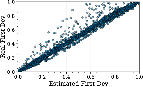
Figure 2: First derivative estimation

These Copulas have a single parameter, which we varied. Gaussian Copulas ($\rho$) has a correlation parameter, and we set it to: 0.1, 0.5, and 0.9. Clayton and Frank copulas’ mixing parameter ($\theta$) was set to 1, 5, and 10. For each of these configurations, we measured the coefficient of determination ($R2$) between empirical estimates and exact formulae. One example of such an estimate for a Frank Copula with $\theta=10$ is shown in Figure 2. Overall, we found that R2 was above $0.899$ in every setting, validating our approach.

5.2 2-Cats on Synthetic Data

We now turn to our results on synthetic datasets. Our primary focus, as is the case on baseline methods, will be on capturing the data likelihood:

$$f(x_{1},x_{2})=f(x_{1})\,f(x_{2})\,c(F^{-1}(x_{1}),F^{-1}(x_{2}))$$

For both 2-Cats models, we estimate this density as:

$$f(x_{1},x_{2})\approx k_{1}(x_{1})\,k_{2}(x_{2})\,\frac{\partial^{2}H_{\bm{\theta}}(u,v)}{\partial u\partial v}$$

Here, $k_{1}(x_{1})$ and $k_{2}(x_{2})$ are KDE models for the PDFs for $X_{1}$ and $X_{2}$ respectivelly. The bandwidth for these methods is determined using Silverman’s rule [Silverman, 1986].

As is commonly done, we evaluate the natural log of this quantity as the data log-likelihood and use its negative to compare 2-Cats with other methods. With this metric of interest in place, we considered two 2-Cats models:

1. 2-Cats-G (Final Layer Gaussian): 2-Cats with a Gaussian bivariateCDF as $G$.

2. 2-Cats-L (Final Layer Logistic): 2-Cats with a Logistic bivariateCDF as $G$.

Thus, we considered two forms of $G$. The first was the CDF of a bivariate Gaussian Distribution [Tsay and Ke, 2023]. The second one is the CDF of the Flexible bivariate Logistic (see Section 11.8 of Arnold [1992]):

$$F(x_{1},x_{2})=\Pr[X_{1}<x_{1},X_{2}<x_{2}]=$$

$$\big{(}(1+e^{-\alpha\frac{x_{1}-\mu_{1}}{\sigma_{1}}}+e^{-\alpha\frac{x_{2}-\mu_{2}}{\sigma_{2}}}+e^{-\alpha(\frac{x_{1}-\mu_{1}}{\sigma_{1}}+\frac{x_{2}-\mu_{2}}{\sigma_{2}})})^{\frac{1}{\alpha}}\big{)}^{-1}$$

$\mu_{1}$, $\mu_{2}$, $\sigma_{1}$, $\sigma_{2}$ and $\alpha$ are free parameters optimized by the model. The same goes for the free parameters of the bivariate Gaussian CDF (the means of each dimension, $\mu_{1}$ and $\mu_{2}$, and the correlation parameter $\rho$). Moreover, for each model, we employed four-layer networks with hidden layers having sizes of 128, 64, 32, and 16. We now discuss loss weights.

Recall that the data density is proportional to the pseudo-likelihood. We primarily emphasized the likelihood loss ($w^{c}$). This accentuates our pivotal component. Notably, the scale of its values differs from that of the MSE components, necessitating a proportional adjustment in weight selection. In light of these factors, we fixed $w^{C}=0.01$, $w^{dC}=0.5$, and $w^{c}=0.1$. We note that these hyper-parameters were sufficient to show how our approach is better than the literature. Thus, no exhaustive grid search was needed.

Our models were trained using early stopping. Here, for each training epoch, we evaluated the pseudo-log-likelihood on the training set and kept the weights of the epoch with the best likelihood on the training dataset.

Table 1: Results for Synthetic Data. Copula parameters are shown on the header. Marginals come from two Normal distributions ($\mu=0,\sigma=1$). $95\%$ confidence intervals (bootstrap) show. Green indicates that a 2-Cats model was, on average, better than the best baseline (indicated by Red). Underscores highlight the best statistical ties with the best model.

Gaussian ($\rho$) Clayton ($\theta$) Frank/Joe ($\theta$) 0.1 0.5 0.9 1 5 10 1 5 10 Non-Deep Learn Par $-0.55\pm 0.12$ $-0.55\pm 0.13$ $-0.55\pm 0.16$ $-1.12\pm 0.09$ $-1.12\pm 0.16$ $-1.12\pm 0.21$ $-0.86\pm 0.09$ $-0.86\pm 0.12$ $-0.86\pm 0.15$ Bern $-0.54\pm 0.12$ $-0.54\pm 0.13$ $-0.54\pm 0.14$ $-1.10\pm 0.08$ $-1.10\pm 0.12$ $-1.10\pm 0.18$ $-0.85\pm 0.09$ $-0.85\pm 0.12$ $-0.85\pm 0.14$ PBern $-0.55\pm 0.11$ $-0.55\pm 0.14$ $-0.55\pm 0.14$ $-1.11\pm 0.08$ $-1.11\pm 0.12$ $-1.11\pm 0.18$ $-0.86\pm 0.09$ $-0.86\pm 0.13$ $-0.86\pm 0.15$ PSPL1 $-0.55\pm 0.11$ $-0.55\pm 0.13$ $-0.55\pm 0.14$ $-1.11\pm 0.07$ $-1.11\pm 0.15$ $-1.11\pm 0.30$ $-0.86\pm 0.09$ $-0.86\pm 0.12$ $-0.86\pm 0.18$ PSPL2 $-0.55\pm 0.11$ $-0.55\pm 0.13$ $-0.55\pm 0.15$ $-1.10\pm 0.08$ $-1.10\pm 0.14$ $-1.10\pm 0.24$ $-0.86\pm 0.09$ $-0.86\pm 0.12$ $-0.86\pm 0.17$ TTL0 $-0.54\pm 0.12$ $-0.54\pm 0.14$ $-0.54\pm 0.15$ $-1.11\pm 0.09$ $-1.11\pm 0.16$ $-1.11\pm 0.27$ $-0.86\pm 0.08$ $-0.86\pm 0.13$ $-0.86\pm 0.16$ TLL1 $-0.53\pm 0.12$ $-0.53\pm 0.14$ $-0.53\pm 0.16$ $-1.12\pm 0.08$ $-1.12\pm 0.17$ $-1.12\pm 0.32$ $-0.85\pm 0.09$ $-0.85\pm 0.12$ $-0.85\pm 0.17$ TLL2 $-0.54\pm 0.12$ $-0.54\pm 0.14$ $-0.54\pm 0.15$ $-1.12\pm 0.09$ $-1.12\pm 0.19$ $-1.12\pm 0.40$ $-0.86\pm 0.09$ $-0.86\pm 0.13$ $-0.86\pm 0.16$ TLL2nn $-0.55\pm 0.12$ $-0.55\pm 0.14$ $-0.55\pm 0.15$ $-1.12\pm 0.08$ $-1.12\pm 0.17$ $-1.12\pm 0.40$ $-0.86\pm 0.09$ $-0.86\pm 0.13$ $-0.86\pm 0.15$ MR $-0.54\pm 0.12$ $-0.54\pm 0.13$ $-0.54\pm 0.14$ $-1.08\pm 0.08$ $-1.08\pm 0.14$ $-1.08\pm 0.34$ $-0.84\pm 0.09$ $-0.84\pm 0.12$ $-0.84\pm 0.15$ Probit $-0.55\pm 0.12$ $-0.55\pm 0.13$ $-0.55\pm 0.15$ $-1.10\pm 0.08$ $-1.10\pm 0.14$ $-1.10\pm 0.29$ $-0.85\pm 0.09$ $-0.85\pm 0.12$ $-0.85\pm 0.16$ Deep Learn ACNet $-0.06\pm 0.09$ $-0.29\pm 0.09$ $-1.05\pm 0.08$ $-0.51\pm 0.07$ $-0.91\pm 0.11$ $-1.35\pm 0.04$ $-0.13\pm 0.09$ $-0.49\pm 0.08$ $-0.58\pm 0.10$ GEN-AC $-0.06\pm 0.08$ $-0.29\pm 0.08$ $-1.06\pm 0.07$ $-0.52\pm 0.06$ $-0.93\pm 0.12$ $-1.34\pm 0.05$ $-0.15\pm 0.07$ $-0.49\pm 0.08$ $-0.56\pm 0.10$ NL $-0.34\pm 0.09$ $-0.43\pm 0.07$ $-1.07\pm 0.07$ $-0.64\pm 0.07$ $-1.17\pm 0.13$ $-1.03\pm 0.07$ $-0.42\pm 0.07$ $-0.59\pm 0.08$ $-0.57\pm 0.06$ IGC $-0.58\pm 0.07$ $-0.67\pm 0.06$ $-0.86\pm 0.06$ $-0.66\pm 0.06$ $-0.88\pm 0.06$ $-0.83\pm 0.06$ $-0.66\pm 0.06$ $-0.73\pm 0.05$ $-0.75\pm 0.07$ Our 2-Cats-L $-0.48\pm 0.14$ $-0.63\pm 0.13$ $-1.20\pm 0.23$ $-0.64\pm 0.14$ $-1.24\pm 0.20$ $-1.69\pm 0.19$ $-0.52\pm 0.17$ $-1.34\pm 0.17$ $-1.34\pm 0.14$ 2-Cats-G $-0.38\pm 0.15$ $-0.45\pm 0.19$ $-1.04\pm 0.28$ $-0.44\pm 0.19$ $-1.27\pm 0.30$ $-1.06\pm 0.18$ $-0.51\pm 0.15$ $-1.12\pm 0.09$ $-1.06\pm 0.18$

In both our synthetic and real data experiments, we considered the following approaches as Deep Learning baselines: Deep Archimedian Copulas (ACNET) [Ling et al., 2020]; Generative Archimedian Copulas (GEN-AC) [Ng et al., 2021]; Neural Likelihoods (NL) [Chilinski and Silva, 2020]; and Implicit Generative Copulas (IGC) [Janke et al., 2021]. ACNET, GEN-AC, and IGC are all methods focused on Copulas. ACNET, GEN-AC, and IGC present experiments for bivariate data on their studies. Here, we use the same hyperparameters employed by the authors. This is also true for NL, but the authors did not present an analysis of synthetic Copula datasets or bivariate data in their study. We consider NL a baseline given that it presents a similar idea to ours: employ monotonic NNs.

We also considered several Non-Deep Learning baselines. These were the Parametric and Non-Parametric Copula Models from Nagler et al. [2017]. They are referenced as: The best Parametric approach from several known parametric copulas (Par), non-penalized Bernstein estimator (Bern), penalized Bernstein estimator (PBern), penalized linear B-spline estimator (PSPL1), penalized quadratic B-spline estimator (PSPL2), transformation local likelihood kernel estimator of degree $q=0$ (TTL0), degree $q=1$ (TTL1), and $q=2$ (TTL2), and $q=2$ with nearest neughbors (TTL2nn). We also considered the recent non-parametric approach by Mukhopadhyay and Parzen [Mukhopadhyay and Parzen, 2020] (MR), as well as the Probit transformation-based estimator from Geenens et al. [2017]. These approaches have R code on the CRAN (see Appendix E).

To assess the performance of our model on synthetic bivariate datasets, we generated Gaussian copulas with correlations $\rho=0.1,0.5,0.9$, and Clayton and Frank copulas with parameters $\theta=1,5,10$. The marginal distributions were chosen as uncorrelated Normal distributions with parameters ($\mu=0,\sigma=1$). We generated 1,500 training samples and 500 test samples. Results are for test samples.

The results are presented in Table 1, which contains the average negative log-likelihood on the test set for each copula. Results were estimated with a fixed seed of 30091985. The table also shows 95% Bootstrap Confidence Intervals [Wasserman, 2004]. Following suit with several guidelines, we choose to report CIs for better interpretability on the expected range of scores when replicating our studies [Gardner and Altman, 1986, Sterne and Smith, 2001, Altman et al., 2013, Ho et al., 2019, Dragicevic, 2016, Greenland et al., 2016, Imbens, 2021]. With 95% probability, a change of splits/seeds should achieve an average negative log-likelihood within the reported range.

The winning 2-Cats models are highlighted in the table in Green. The best, on average, baseline methods are in Red. We consider a method better or worse than another when their confidence intervals do not overlap; thus, ties with the best model are shown in underscores. The table shows that 2-Cats is better than baseline methods when the dependency ($\rho$ or $\theta$) increases. For small dependencies, methods not based on Deep Learning outperform Deep ones (including 2-Cats). Nevertheless, 2-Cats is the winning method in 6 out of 9 datasets and is tied with the best in one other column.

5.3 2-Cats on Real Data

Table 2: Negative log-likelihood on real datasets. $95\%$ confidence intervals (bootstrap) show. Green indicates that 2-Cats was, on average, better than the best baseline (indicated in Red). Underscores highlight ties with best model.

		Boston	INTC-MSFT	GOOG-FB
Non-Deep Learn	Par	$-0.16\pm 0.09$	$-0.05\pm 0.07$	$-0.88\pm 0.08$
	Bern	$-0.09\pm 0.06$	$-0.03\pm 0.05$	$-0.70\pm 0.04$
	PBern	$-0.11\pm 0.07$	$-0.02\pm 0.06$	$-0.62\pm 0.04$
	PSPL1	$-0.06\pm 0.14$	$-0.02\pm 0.06$	$-0.72\pm 0.14$
	PSPL2	$-0.05\pm 0.14$	$-0.02\pm 0.06$	$-0.83\pm 0.07$
	TTL0	$-0.16\pm 0.08$	$-0.06\pm 0.06$	$-1.00\pm 0.07$
	TTL1	$-0.18\pm 0.09$	$-0.06\pm 0.06$	$-1.00\pm 0.08$
	TTL2	$-0.18\pm 0.09$	$-0.06\pm 0.06$	$-0.71\pm 0.16$
	TLL2	$-0.15\pm 0.09$	$-0.04\pm 0.05$	$-0.95\pm 0.13$
	MR	$-0.07\pm 0.06$	$-0.01\pm 0.05$	$-0.84\pm 0.07$
	Probit	$-0.10\pm 0.06$	$-0.03\pm 0.07$	$-0.92\pm 0.06$
Deep Learn	ACNet	$-0.28\pm 0.11$	$-0.18\pm 0.08$	$-0.91\pm 0.12$
	GEN-AC	$-0.29\pm 0.11$	$-0.17\pm 0.07$	$-0.75\pm 0.10$
	NL	$-0.28\pm 0.16$	$-0.16\pm 0.08$	$-1.09\pm 0.13$
	IGC	$0.07\pm 0.08$	$0.14\pm 0.04$	$-0.30\pm 0.02$
Our	2-Cats-L	$-0.30\pm 0.09$	$-0.21\pm 0.05$	$-1.75\pm 0.04$
	2-Cats-G	$-0.27\pm 0.07$	$-0.07\pm 0.06$	$-1.65\pm 0.08$

As was done in previous work, we employ the Boston housing dataset, the Intel-Microsoft (INTC-MSFT), and Google-Facebook (GOOG-FB) stock ratios. These pairs are commonly used in Copula research; in particular, they are the same datasets used by [Ling et al., 2020, Ng et al., 2021]. We employed the same train/test and pre-processing as previous work for fair comparisons.

The results are presented in Table 2, again highlighting the superior performance of the 2-Cats models across all datasets. Only in one setting did the model underperform when compared with the literature. When we cross-reference results on synthetic and natural datasets, 2-Cats present’s itself as a promising novel approach to model Copulas.

6 Conclusions

In this paper, we presented Copula Approximating Transform models (2-Cats). Different from the literature when training our models; we focus not only on capturing the pseudo-likelihood of Copulas but also on several other properties, such as the partial derivatives of the $C$ function. We prove that our models are valid Copulas and thus useful for pairwise data modeling. Moreover, a second major innovation is proposing estimators that employ using Sobolev training. Overall, our results show the superiority of variations of 2-Cats on synthetic and real datasets.

A natural follow-up for 2-Cats is on using the Pair Copula Construction (PCC) [Aas et al., 2009, Czado, 2010] to port Vines [Czado and Nagler, 2022, Low et al., 2018, Genest et al., 1995, Genest and Favre, 2007] to incorporate our method. PCC is a well-established algorithm to go from a 2D Copula to an ND One using Vines. Our focus on the main text of this paper was on showing 2-Cats as a valid 2D approach.

We also believe that evaluating other non-negative NNs for $m_{\bm{\theta}}$ is a promising direction [Marteau-Ferey et al., 2020, Rudi and Ciliberto, 2021, Tsuchida et al., 2023, Sladek et al., 2023, Loconte et al., 2023, Kortvelesy, 2023].

We point out that before reaching our 2-Cats model, several variations of the model were considered. We refer the reader to Appendix D for results and details of such variations.

Appendix A Sampling from 2-Cats

We now detail how to sample from 2-Cats. Let the first derivatives of 2-Cats be: $h_{v}(u)=\Pr[U\leq u\mid V=v]=\frac{\partial H_{\bm{\theta}}(u,v)}{\partial v}$, and $h_{u}(v)=\Pr[V\leq v\mid U=u]=\frac{\partial H_{\bm{\theta}}(u,v)}{\partial u}$. Now, let $h^{\prime}_{v}(u)=\frac{\partial^{2}H_{\bm{\theta}}(u,v)}{\partial v^{2}}$ be the first derivative of $h_{v}(u)$, and similarly $h^{\prime}_{u}(v)=\frac{\partial^{2}H_{\bm{\theta}}(u,v)}{\partial u^{2}}$. These derivatives are readily available in the Hessian matrix that we estimate symbolically for 2-Cats (see Section 3).

Now, let us determine the inverse of $h_{u}(v)$, that is: $h^{-1}_{u}(v_{i})$ (the subscript stands for inverse). The same arguments are valid for $h_{v}(u)$ and $h^{-1}_{v}(u_{i})$, and thus we omit them. Notice that with this inverse, we can sample from the CDF defined by $h_{u}(v)$ using the well-known Inverse transform sampling. Now, notice that by definition, $h_{u}(v)$ is already the derivative of $H_{\bm{\theta}}(u,v)$ with regards to $u$.

Using a Legendre transform, the inverse of a derivative is:

$$h^{-1}_{u}(v_{i})=\big{(}h^{\prime}_{u}(v_{i})\big{)}^{-1}=\big{(}\frac{\partial^{2}H_{\bm{\theta}}(u,v_{i})}{\partial u^{2}}\big{)}^{-1}$$

Where, again, the derivative inside the parenthesis is readily available to us via symbolic computation.

With such results in hand, the algorithm for sampling is:

1. Generate two independent values $u\sim Uniform(0,1)$ and $v_{i}\sim Uniform(0,1)$.

2. Set $v=h^{-1}_{u}(v_{i})$. This is an Inverse transform sampling for $v$

3. Now we have the $(u,v)$ pair. We can again use Inverse transform sampling to determine:

   1. $x_{1}=F^{-1}_{x_{1}}(u)$

   2. $x_{2}=F^{-1}_{x_{2}}(v)$

Appendix B A Mixture of 2-Cats is a Universal Copula Approximator

With sufficient components, any other CDF (or density function) may be approximated by a mixture of other CDFs [Nguyen et al., 2020]. As a consequence, a mixture of 2-Cats of the form:

$$H_{\bm{m},\bm{\Theta}}(u,v)=\sum_{i=1}^{k}w_{i}H_{i,\bm{\theta_{i}}}(u,v),$$

where $H_{i,\bm{\theta_{i}}}(u,v)$ is the $i$-th 2-Cats model. $\bm{\Theta}$ is the parameter vector comprised of concatenating the individual parameters of each mixture component: $\bm{\Theta}=[\bm{\theta_{1}},\bm{\theta_{2}},\dots,\bm{\theta_{k}}]$, and $\bm{m}=[m_{1},m_{2},\dots m_{k}]$ are real numbers related to the mixture weights.

This model may be trained as follows:

1. Map mixture parameters to the $k-1$ Simplex: $\mathbf{w}=\text{softmax}(\bm{\theta}_{w})$. $w_{i}$ if the $i$-th position of this vector.

2. When training, backpropagate to learn $\bm{\Theta}$ and $\bm{m}$.

This is similar to the Mixture Density NN [Bishop, 1994]. Over the last few years, mixture of Copulas approaches has been gaining traction in several fields [Abraj et al., 2022, Sohrabian, 2021, Zhang and Shi, 2017]; here, we are proposing an NN variation. By definition, this is a valid Copula.

Appendix C On the Integral of Neural Networks

Let $\hat{f}_{\bm{\theta}}(x)$ be some NN parametrized by $\bm{\theta}$. Also, let $f(x)$ represent our training dataset. We also make the reasonable assumption our dataset comes from some real function, $f^{\ast}(x)$, sampled under a symmetric additive noise, i.e., $f(x)=f^{\ast}(x)+\eta$, with an expected value equal to zero: $\mathbb{E}[\eta]=0$. Gaussian noise is such a case.

If a NN is a universal approximator Cybenko [1989], Hornik et al. [1989], Lu et al. [2021], Cai [2023], Lu et al. [2017] and it is trained on the dataset $f(x)$, we have that:

$$\lVert\hat{f}_{\bm{\theta}}(x)-f(x)\rVert_{p}<\epsilon_{1}$$

Most UAT proofs are valid for any $p$ norm ($p$ norms bound one another), and assuming the 1 norm, we reach: $\hat{f}_{\bm{\theta}}(x)=f(x)\pm\epsilon$ for some constant $\epsilon$. As a consequence, we shall reach the following relationship:

$$\hat{f}_{\bm{\theta}}(x)=f^{\ast}(x)+\eta\pm\epsilon_{1}$$

Given that integration is a linear operator, we can show that:

$$\int\hat{f}_{\bm{\theta}}(x)=\int f^{\ast}(x)+\int\eta\pm\int\epsilon_{1}=\int f^{\ast}(x)\pm\epsilon_{2}$$

Here, $\int\eta=0$ as $\eta$ is symmetric with mean $0$. $\epsilon_{2}$ is a second error variable that arises from integrating a constant. It will be in the order of the integrating variable, i.e., $\epsilon_{2}=O(x)$ if integrating on $x$. Controlling for $\epsilon_{2}$ will depend on the dataset’s quality and the training procedure. This is one more reason why we regularize our networks, as is done in PINNs.

A similar result is discussed in Liu [2023].

Appendix D A Flexible Variation of the Model

A Flexible 2-Cats model works similarly to our 2-Cats. However, the transforms are different:

1. Let $m_{\bm{\theta}}:\mathbb{I}^{2}\mapsto\mathbb{R}+$ be an MLP outputs positive numbers. We achieve this by employing Elu plus one activation in every layer as in Wehenkel and Louppe [2019].

2. Define the transforms:

   $$t_{v}(u)=\int_{0}^{u}m_{\bm{\theta}}(x,v)\,dx;\,\,t_{u}(v)=\int_{0}^{v}m_{\bm{\theta}}(y,u))\,dy.$$

3. The 2-Cats-FLEX hypothesis is now defined as the function: $H_{\bm{\theta}}(u,v)=G\big{(}(t_{v}(u),t_{u}(v)\big{)}$, where $G(x,y)$ is any bivariate CDF on the $\mathbb{R}^{2}$ domain (e.g., the Bivariate Logistic or Bivariate Gaussian).

This model meets P3, but not P1 nor P2. As already stated in the introduction, the fact that $t_{v}(u)$ and $t_{u}(v)$ are monotonic, one-to-one, guarantees that $G(t_{v}(u),t_{u}(v))$ defines a valid probability transform to a new CDF. A major issue with this approach is that we have no guarantee that the model’s derivatives are conditional cumulative functions (first derivatives) or density functions (second derivatives). That’s why we call it Flexible (FLEX).

D.1 Full Results

Table 3: Negative log-likelihood on real datasets. $95\%$ confidence intervals (bootstrap) show. Green indicates that a 2-Cats model was better than the best baseline (indicated in Red). Underscores highlight ties with best model.

	Boston	INTC-MSFT	GOOG-FB
Par	$-0.16\pm 0.09$	$-0.05\pm 0.07$	$-0.88\pm 0.08$
Bern	$-0.09\pm 0.06$	$-0.03\pm 0.05$	$-0.70\pm 0.04$
PBern	$-0.11\pm 0.07$	$-0.02\pm 0.06$	$-0.62\pm 0.04$
PSPL1	$-0.06\pm 0.14$	$-0.02\pm 0.06$	$-0.72\pm 0.14$
PSPL2	$-0.05\pm 0.14$	$-0.02\pm 0.06$	$-0.83\pm 0.07$
TTL0	$-0.16\pm 0.08$	$-0.06\pm 0.06$	$-1.00\pm 0.07$
TTL1	$-0.18\pm 0.09$	$-0.06\pm 0.06$	$-1.00\pm 0.08$
TTL2	$-0.18\pm 0.09$	$-0.06\pm 0.06$	$-0.71\pm 0.16$
TLL2	$-0.15\pm 0.09$	$-0.04\pm 0.05$	$-0.95\pm 0.13$
MR	$-0.07\pm 0.06$	$-0.01\pm 0.05$	$-0.84\pm 0.07$
Probit	$-0.10\pm 0.06$	$-0.03\pm 0.07$	$-0.92\pm 0.06$
ACNet	$-0.28\pm 0.11$	$-0.18\pm 0.08$	$-0.91\pm 0.12$
GEN-AC	$-0.29\pm 0.11$	$-0.17\pm 0.07$	$-0.75\pm 0.10$
NL	$-0.28\pm 0.16$	$-0.16\pm 0.08$	$-1.09\pm 0.13$
IGC	$0.07\pm 0.08$	$0.14\pm 0.04$	$-0.30\pm 0.02$
2-Cats-FLEX-L	$0.38\pm 0.71$	$0.19\pm 0.08$	$-1.15\pm 0.07$
2-Cats-FLEX-G	$0.50\pm 0.43$	$0.23\pm 0.09$	$-1.01\pm 0.07$
2-Cats-G	$-0.30\pm 0.09$	$-0.21\pm 0.05$	$-1.75\pm 0.04$
2-Cats-L	$-0.27\pm 0.07$	$-0.07\pm 0.06$	$-1.65\pm 0.08$

In Table 3, we show the results for these models on real datasets. The definitions of the models are as follows: (2-Cats-P Gaus.) A parametric mixture of 10 Gaussian Copula densities.; (2-Cats-P Frank) Similar to the above, but is a mixture of 10 Frank Copula densities; (2-Cats-FLEX-G) A Flexible model version where the final activation layer is Bivariate Gaussian CDF; (2-Cats-FLEX-L) A Flexible version of the model where the final activation layer is Bivariate Logistic CDF.

Models were trained with the same hyperparameters and network definition as the ones in our main text.

Appendix E Appendix Baseline Source Code

Table 4: Source Code Used as Baselines

		Link
Non-Deep Learn	Par	https://cran.r-project.org/web/packages/VineCopula/index.html
	Bern	https://cran.r-project.org/web/packages/kdecopula/index.html
	PBern	https://rdrr.io/cran/penRvine/
	PSPL1	https://rdrr.io/cran/penRvine/
	PSPL2	https://rdrr.io/cran/penRvine/
	TTL0	https://cran.r-project.org/web/packages/kdecopula/index.html
	TTL1	https://cran.r-project.org/web/packages/kdecopula/index.html
	TTL2	https://cran.r-project.org/web/packages/kdecopula/index.html
	TLL2	https://cran.r-project.org/web/packages/kdecopula/index.html
	MR	https://cran.r-project.org/web/packages/kdecopula/index.html
	Probit	https://cran.r-project.org/web/packages/kdecopula/index.html
Deep Learn	ACNet	https://github.com/lingchunkai/ACNet
	GEN-AC	https://github.com/yutingng/gen-AC
	NL	https://github.com/pawelc/NeuralLikelihoods0
	IGC	https://github.com/TimCJanke/igc

The links for baseline source code are in Table 4.

References

- Aas et al. [2009] Kjersti Aas, Claudia Czado, Arnoldo Frigessi, and Henrik Bakken. Pair-copula constructions of multiple dependence. Insurance: Mathematics and economics, 44(2), 2009.
- Abraj et al. [2022] Mohomed Abraj, You-Gan Wang, and M Helen Thompson. A new mixture copula model for spatially correlated multiple variables with an environmental application. Scientific Reports, 12(1), 2022.
- Altman et al. [2013] Douglas Altman, David Machin, Trevor Bryant, and Martin Gardner. Statistics with confidence: confidence intervals and statistical guidelines. John Wiley & Sons, 2013.
- Arnold [1992] Barry C Arnold. Multivariate logistic distributions. Marcel Dekker New York, 1992.
- Bakam and Pommeret [2023] Yves I Ngounou Bakam and Denys Pommeret. Nonparametric estimation of copulas and copula densities by orthogonal projections. Econometrics and Statistics, 2023.
- Bishop [1994] Christopher M Bishop. Mixture density networks. Online Report., 1994.
- Cai [2023] Yongqiang Cai. Achieve the minimum width of neural networks for universal approximation. In ICLR, 2023.
- Casella and Berger [2001] George Casella and Roger L Berger. Statistical inference. Cengage Learning, 2001.
- Cherubini et al. [2004] Umberto Cherubini, Elisa Luciano, and Walter Vecchiato. Copula methods in finance. John Wiley & Sons, 2004.
- Chilinski and Silva [2020] Pawel Chilinski and Ricardo Silva. Neural likelihoods via cumulative distribution functions. In UAI, 2020.
- Cybenko [1989] George Cybenko. Approximation by superpositions of a sigmoidal function. Mathematics of control, signals, and systems, 2(4), 1989.
- Czado [2010] Claudia Czado. Pair-copula constructions of multivariate copulas. In Copula Theory and Its Applications. Springer, 2010.
- Czado and Nagler [2022] Claudia Czado and Thomas Nagler. Vine copula based modeling. Annual Review of Statistics and Its Application, 9, 2022.
- Czarnecki et al. [2017] Wojciech M Czarnecki, Simon Osindero, Max Jaderberg, Grzegorz Swirszcz, and Razvan Pascanu. Sobolev training for neural networks. In NeurIPS, 2017.
- Daniels and Velikova [2010] Hennie Daniels and Marina Velikova. Monotone and partially monotone neural networks. IEEE Transactions on Neural Networks, 21(6), 2010.
- Dragicevic [2016] Pierre Dragicevic. Fair statistical communication in hci. Modern statistical methods for HCI, 2016.
- Gardner and Altman [1986] Martin Gardner and Douglas Altman. Confidence intervals rather than p values: estimation rather than hypothesis testing. Br Med J (Clin Res Ed), 292(6522), 1986.
- Geenens et al. [2017] Gery Geenens, Arthur Charpentier, and Davy Paindaveine. Probit transformation for nonparametric kernel estimation of the copula density. Bernoulli, 2017.
- Genest and Favre [2007] Christian Genest and Anne-Catherine Favre. Everything you always wanted to know about copula modeling but were afraid to ask. Journal of hydrologic engineering, 12(4), 2007.
- Genest et al. [1995] Christian Genest, Kilani Ghoudi, and L-P Rivest. A semiparametric estimation procedure of dependence parameters in multivariate families of distributions. Biometrika, 82(3), 1995.
- Greenland et al. [2016] Sander Greenland, Stephen J Senn, Kenneth J Rothman, John B Carlin, Charles Poole, Steven N Goodman, and Douglas G Altman. Statistical tests, p values, confidence intervals, and power: a guide to misinterpretations. European journal of epidemiology, 31, 2016.
- Größer and Okhrin [2022] Joshua Größer and Ostap Okhrin. Copulae: An overview and recent developments. Wiley Interdisciplinary Reviews: Computational Statistics, 14(3), 2022.
- Hirt et al. [2019] Marcel Hirt, Petros Dellaportas, and Alain Durmus. Copula-like variational inference. In NeurIPS, 2019.
- Ho et al. [2019] Joses Ho, Tayfun Tumkaya, Sameer Aryal, Hyungwon Choi, and Adam Claridge-Chang. Moving beyond p values: data analysis with estimation graphics. Nature methods, 16(7), 2019.
- Hornik et al. [1989] Kurt Hornik, Maxwell Stinchcombe, and Halbert White. Multilayer feedforward networks are universal approximators. Neural networks, 2(5), 1989.
- Imbens [2021] Guido W Imbens. Statistical significance, p-values, and the reporting of uncertainty. Journal of Economic Perspectives, 35(3), 2021.
- Janke et al. [2021] Tim Janke, Mohamed Ghanmi, and Florian Steinke. Implicit generative copulas. In NeurIPS, 2021.
- Karniadakis et al. [2021] George Em Karniadakis, Ioannis G Kevrekidis, Lu Lu, Paris Perdikaris, Sifan Wang, and Liu Yang. Physics-informed machine learning. Nature Reviews Physics, 3(6), 2021.
- Kobyzev et al. [2020] Ivan Kobyzev, Simon JD Prince, and Marcus A Brubaker. Normalizing flows: An introduction and review of current methods. IEEE transactions on pattern analysis and machine intelligence, 43(11), 2020.
- Kortvelesy [2023] Ryan Kortvelesy. Fixed integral neural networks. arXiv preprint arXiv:2307.14439, 2023.
- Ling et al. [2020] Chun Kai Ling, Fei Fang, and J Zico Kolter. Deep archimedean copulas. In NeurIPS, 2020.
- Liu [2023] Yucong Liu. Neural networks are integrable. arXiv preprint arXiv:2310.14394, 2023.
- Loconte et al. [2023] Lorenzo Loconte, Stefan Mengel, Nicolas Gillis, and Antonio Vergari. Negative mixture models via squaring: Representation and learning. In The 6th Workshop on Tractable Probabilistic Modeling, 2023.
- Low et al. [2018] Rand Kwong Yew Low, Jamie Alcock, Robert Faff, and Timothy Brailsford. Canonical vine copulas in the context of modern portfolio management: Are they worth it? Asymmetric Dependence in Finance: Diversification, Correlation and Portfolio Management in Market Downturns, 2018.
- Lu et al. [2021] Lu Lu, Raphael Pestourie, Wenjie Yao, Zhicheng Wang, Francesc Verdugo, and Steven G Johnson. Physics-informed neural networks with hard constraints for inverse design. SIAM Journal on Scientific Computing, 43(6), 2021.
- Lu and Lu [2020] Yulong Lu and Jianfeng Lu. A universal approximation theorem of deep neural networks for expressing probability distributions. In NeurIPS, 2020.
- Lu et al. [2017] Zhou Lu, Hongming Pu, Feicheng Wang, Zhiqiang Hu, and Liwei Wang. The expressive power of neural networks: A view from the width. In NeurIPS, 2017.
- Marteau-Ferey et al. [2020] Ulysse Marteau-Ferey, Francis Bach, and Alessandro Rudi. Non-parametric models for non-negative functions. In NeurIPS, 2020.
- Modiri et al. [2020] Sadegh Modiri, Santiago Belda, Mostafa Hoseini, Robert Heinkelmann, José M Ferrándiz, and Harald Schuh. A new hybrid method to improve the ultra-short-term prediction of lod. Journal of geodesy, 94, 2020.
- Mukhopadhyay and Parzen [2020] Subhadeep Mukhopadhyay and Emanuel Parzen. Nonparametric universal copula modeling. Applied Stochastic Models in Business and Industry, 36(1), 2020.
- Naaman [2021] Michael Naaman. On the tight constant in the multivariate dvoretzky–kiefer–wolfowitz inequality. Statistics & Probability Letters, 173, 2021.
- Nagler et al. [2017] Thomas Nagler, Christian Schellhase, and Claudia Czado. Nonparametric estimation of simplified vine copula models: comparison of methods. Dependence Modeling, 5(1), 2017.
- Nelsen [2006] Roger B Nelsen. An introduction to copulas. Springer, 2006.
- Ng et al. [2021] Yuting Ng, Ali Hasan, Khalil Elkhalil, and Vahid Tarokh. Generative archimedean copulas. In UAI, 2021.
- Nguyen et al. [2020] T Tin Nguyen, Hien D Nguyen, Faicel Chamroukhi, and Geoffrey J McLachlan. Approximation by finite mixtures of continuous density functions that vanish at infinity. Cogent Mathematics & Statistics, 7(1), 2020.
- Papamakarios et al. [2017] George Papamakarios, Theo Pavlakou, and Iain Murray. Masked autoregressive flow for density estimation. In NeurIPS, 2017.
- Rudi and Ciliberto [2021] Alessandro Rudi and Carlo Ciliberto. Psd representations for effective probability models. In NeurIPS, 2021.
- Salvadori and De Michele [2004] G Salvadori and Carlo De Michele. Frequency analysis via copulas: Theoretical aspects and applications to hydrological events. Water resources research, 40(12), 2004.
- Schepsmeier and Stöber [2014] Ulf Schepsmeier and Jakob Stöber. Derivatives and fisher information of bivariate copulas. Statistical papers, 55(2), 2014.
- Sill [1997] Joseph Sill. Monotonic networks. In NeurIPS, 1997.
- Silverman [1986] Bernard W Silverman. Density estimation for statistics and data analysis, volume 26. CRC press, 1986.
- Sklar [1996] Abe Sklar. Random variables, distribution functions, and copulas: a personal look backward and forward. Lecture notes-monograph series, 1996.
- Sklar [1959] M Sklar. Fonctions de répartition à n dimensions et leurs marges. Annales de l’ISUP, 8(3), 1959.
- Sladek et al. [2023] Aleksanteri Mikulus Sladek, Martin Trapp, and Arno Solin. Encoding negative dependencies in probabilistic circuits. In The 6th Workshop on Tractable Probabilistic Modeling, 2023.
- Sohn et al. [2015] Kihyuk Sohn, Honglak Lee, and Xinchen Yan. Learning structured output representation using deep conditional generative models. In NeurIPS, 2015.
- Sohrabian [2021] B Sohrabian. Geostatistical prediction through convex combination of archimedean copulas. Spatial Statistics, 41, 2021.
- Sterne and Smith [2001] Jonathan AC Sterne and George Davey Smith. Sifting the evidence—what’s wrong with significance tests? Physical therapy, 81(8), 2001.
- Tagasovska et al. [2023] Natasa Tagasovska, Firat Ozdemir, and Axel Brando. Retrospective uncertainties for deep models using vine copulas. In AISTATS, 2023.
- Tsay and Ke [2023] Wen-Jen Tsay and Peng-Hsuan Ke. A simple approximation for the bivariate normal integral. Communications in Statistics-Simulation and Computation, 52(4), 2023.
- Tsuchida et al. [2023] Russell Tsuchida, Cheng Soon Ong, and Dino Sejdinovic. Squared neural families: A new class of tractable density models. arXiv preprint arXiv:2305.13552, 2023.
- Wasserman [2004] Larry Wasserman. All of statistics: a concise course in statistical inference, volume 26. Springer, 2004.
- Wehenkel and Louppe [2019] Antoine Wehenkel and Gilles Louppe. Unconstrained monotonic neural networks. In NeurIPS, 2019.
- Yang et al. [2019] Liuyang Yang, Jinghuai Gao, Naihao Liu, Tao Yang, and Xiudi Jiang. A coherence algorithm for 3-d seismic data analysis based on the mutual information. IEEE Geoscience and Remote Sensing Letters, 16(6), 2019.
- Zhang and Shi [2017] Qingyang Zhang and Xuan Shi. A mixture copula bayesian network model for multimodal genomic data. Cancer Informatics, 16, 2017.