Meshless interface tracking for the simulation of dendrite envelope growth

Abstract

The growth of dendritic grains during solidification is often modelled using the Grain Envelope Model (GEM), in which the envelope of the dendrite is an interface tracked by the Phase Field Interface Capturing (PFIC) method. In the PFIC method, an phase-field equation is solved on a fixed mesh to track the position of the envelope. While being versatile and robust, PFIC introduces certain numerical artefacts. In this work, we present an alternative approach for the solution of the GEM that employs a Meshless (sharp) Interface Tracking (MIT) formulation, which uses direct, artefact-free interface tracking. In the MIT, the envelope (interface) is defined as a moving domain boundary and the interface-tracking nodes are boundary nodes for the diffusion problem solved in the domain. To increase the accuracy of the method for the diffusion-controlled moving-boundary problem, an h-adaptive spatial discretization is used, thus, the node spacing is refined in the vicinity of the envelope. MIT combines a parametric surface reconstruction, a mesh-free discretization of the parametric surfaces and the space enclosed by them, and a high-order approximation of the partial differential operators and of the solute concentration field using radial basis functions augmented with monomials. The proposed method is demonstrated on a two-dimensional h-adaptive solution of the diffusive growth of dendrite and evaluated by comparing the results to the PFIC approach. It is shown that MIT can reproduce the results calculated with PFIC, that it is convergent and that it can capture more details in the envelope shape than PFIC with a similar spatial discretization.

Novel method for the solution of the Grain Envelope Model (GEM) for dendritic solidification employing sharp interface tracking built on meshless principles.

The new method uses h-adaptive spatial discretization for differential operator approximation and solute concentration field approximation on a moving boundary problem.

Meshless interface tracking (MIT) is numerically more accurate than the interface capturing used in previous work because it uses a conceptually different approach to determine the position of the moving interface and thus avoids numerical artefacts linked to the use of a phase field for interface capturing.

Compared to the interface capturing method, MIT requires less computational nodes to capture all the details in the dendritic envelope shape.

1 Introduction

Dendritic grains are a prevalent type of crystal growth morphology observed in solidification of metallic alloys. They appear widely in solidification processing: additive manufacturing (3D printing), casting, welding, brazing, etc. The size and shape of the grains are a key factor for the properties of the resulting material. Dendritic solidification is controlled by the extraction of latent heat, by diffusion of solute into the liquid surrounding the grains, and by properties of the solid-liquid interface. Therefore it is a multiscale phenomenon and requires the use of models at different scales, ranging from the scale of the dendrite branch (microscopic, typically $10^{-6}\,$m), over the scale of an ensemble of grains (mesoscopic, typically $10^{-3}\,$m) to the process (macroscopic, typically $1\,$m).

At the scale of an ensemble of dendritic grains, the mesoscopic Grain Envelope Model (GEM) [1, 2, 3] is established as a powerful simulation tool. The GEM describes a dendritic grain by its envelope, which is a smooth surface that circumscribes the tips of the growing dendrite branches within a relatively simple shape. The GEM has been used to predict and characterize shapes of equiaxed dendrites [1, 3], solutal interactions between dendrites [4, 2, 5, 6], formation of columnar dendritic patterns [7], and interactions with convection of liquid [8]. Furthermore it has been used for upscaling to macroscopic models: macroscopic constitutive laws of grain growth kinetics have been formulated from GEM simulations of the growth of an ensemble of grains [9]. The capabilities of the GEM to perform quantitative predictions have been assessed extensively by comparisons to experiments and microscopic models [1, 4, 2, 3, 5, 7, 8, 10, 11].

The accuracy of numerical solutions of the GEM [3, 10] is determined primarily by the resolution of the solute concentration in the vicinity of the evolving grain envelope, as well as by the numerical method used to track the envelope. The standard formulations of the GEM  [1, 4, 3] use a phase-field-like interface capturing (PFIC) method [12] to track the grain envelope on a fixed mesh, where the tracked envelope is given by the level set of a continuous phase indicator field. The main advantage of such approach is that it avoids explicit tracking of the envelope and instead propagates the phase field by solving a transport equation on a fixed domain. This results in a relatively straightforward and computationally efficient method that has also been shown to be versatile and robust [12].

There are, however, some drawbacks to using PFIC. In the PFIC approach, the envelope is determined from the continuous field that is propagated by solving the transport equation. Therefore, the propagation speed is not calculated only at the front, but needs to be calculated as a scalar field over the entire domain. This is difficult to do with high accuracy. To achieve sufficient accuracy of the propagation speed calculation for the PFIC, Souhar et al. [3] introduced a front reconstruction technique, which adds significant computational cost to the method. A further aspect requiring particular attention is the tendency of the PFIC to smoothen the envelope [12]. This could in some cases hinder the development of physically significant envelope protrusions, for example such that lead to the formation of new branches of the grain.

If not handled carefully, these aspects can cause undesired numerical artefacts that are potentially detrimental when describing highly non-linear phenomena such as the formation of new branches of the dendrite envelope or the evolution of branches in the initial stages of dendrite growth. It has been shown that the representation of such branching by the GEM remains faithful to the physics [7, 8] but the role of numerical artefacts associated with the envelope tracking method has not yet been verified.

In this paper we explore the possibility to leverage meshless methods [13, 14, 15] to develop an alternative numerical treatment of GEM with the aim of reducing the aforementioned numerical artefacts. One of the key properties of meshless methods is that they operate on unstructured scattered nodes [16], which makes the spatial discretization more flexible and therefore particularly suitable for problems with moving boundaries and problems with high spatial variation in the desired accuracy of the solution [17], both of which apply to GEM.

Instead of using a fixed mesh throughout the simulation and using a phase field to capture the interface, we propose to consider the GEM as a moving boundary problem. In this approach the computational domain is the liquid surrounding the grain and the envelope is a moving boundary, where an appropriate boundary condition for the solution of solute diffusion in the liquid is applied. The envelope is described by boundary nodes that are used both as discretization nodes and as trackers of the envelope motion. In addition, we propose to use an adaptive node refinement [18] that discretizes the solute field on and near the envelope with a much finer node distribution than in the regions far from the envelope. In summary, we propose an alternative numerical solution method for the GEM using an h-adaptive meshless interface tracking (MIT) solution procedure.

Since MIT is an interface tracking method, it avoids the complexity of having to provide a velocity field over the entire domain, as well as computing an additional phase-field equation. Instead, the envelope speed is calculated only on the front, more precisely in the nodes that discretize the envelope. Additionally, the meshless methods — by their design — also provide all the tools necessary to accurately approximate the solute concentration required to compute the envelope velocity. MIT also avoids the smoothing of protrusions, since the envelope is described directly by trackers, thus omitting artefacts induced by a phase field. Finally, the adaptive spatial discretization offers the possibility to describe small radii of curvature on the envelope and also improves the accuracy of the concentration field in the vicinity of the envelope.

In this paper, we first introduce the GEM (Section 2) and we then discuss its standard PFIC solution along with its limitations (Section 3). In the next step (Section 4), we describe the meshless concept and the proposed MIT solution procedure, where we also discuss the expected numerical error for each principal component of the solution procedure separately. In Section 5, the entire solution procedure is verified on a synthetic case of isotropic envelope growth. Finally, in Section 6, we present a GEM simulation of dendritic growth using MIT and we compare the results with PFIC solutions.

2 Mesoscopic Grain Envelope Model (GEM) for equiaxed isothermal solidification

The GEM represents a dendritic grain by its envelope. The dendrite envelope is an artificial smooth surface that connects the tips of the actively growing dendrite branches. The idea behind this simplified representation of a dendrite is that the solute interactions between the grains can be accurately simulated without the need for a detailed representation of the branched structure of the solid-liquid interface. Because of the simplified shape, the computational cost of the GEM is several orders of magnitude smaller than that of models that represent the branched structure of the dendrite in detail [10, 8].

Figure 1 illustrates the key concepts of the GEM. The grain is delimited by the dendrite envelope and its growth is controlled by solute diffusion from the envelope into the adjacent, fully liquid domain. The grain contains both liquid and solid phases. The liquid within the grain and on the envelope is assumed to be in a state of thermodynamic equilibrium. In the case of a binary alloy, this means that the solute concentration is determined by the temperature. In the isothermal system considered in this paper, the temperature is uniform and constant throughout the entire domain (i.e., over several dendrites), resulting in a uniform and constant solute concentration on the envelope. It should be noted that the dimensionless model formulation presented below is only applicable to isothermal solidification, as it assumes a uniform and constant solute concentration on the envelope. More general model descriptions can be found in the literature [2, 8].

Figure 1: Schematic illustration of the main concepts of the GEM.

The GEM assumes that dendrite branches grow in predefined growth directions. The growth speed $v_{n}$ of the dendrite envelope is then given by the speed of the tips $v$ of the dendrite branches by the relation

$$v_{n}=v\cos(\vartheta),$$ (1)

where $\vartheta$ is the smallest of the angles between the outward normal $\boldsymbol{n}$ to the envelope and the individual growth directions of the tips. In the present study, the branches are given $\left\langle 10\right\rangle$ directions, i.e., four possible directions within a two-dimensional domain. The tip speed is calculated from a stagnant-film formulation of the 2D Ivantsov solution [19] which relates the Péclet number Pe of the tip to the normalized dimensionless concentration $u_{\delta}$ of the liquid at a distance $\delta$ from the tip, as

$$u_{\delta}=\sqrt{\pi\text{Pe}}\exp(Pe)\left[\operatorname{erfc}\left(\sqrt{\text{Pe}}\right)-\operatorname{erfc}\left(\sqrt{\text{Pe}+\delta}\right)\right]$$ (2)

and from the so-called tip selection criterion that in dimensionless form reads

$$v=(\text{Pe}/\text{Pe}_{\text{Iv}})^{2},$$ (3)

where $\text{Pe}_{\text{Iv}}$ is a constant. Equations (2) and (3) are used to solve for $v$ at any given point on the envelope. The concentration $u_{\delta}$ is given by the concentration field in the liquid around the envelope, which is resolved numerically from the diffusion equation

$$\frac{\partial u}{\partial t}=\nabla^{2}u.$$ (4)

Equations (1–4) define the GEM, where $\delta$ is a model parameter and $\text{Pe}_{\text{Iv}}$ is a physical parameter, function of the far-field concentration, $u_{0}$. The boundary condition for Equation (4) on the envelope is $u=0$, while the solute diffusion flux across the outer domain boundary is zero, i.e., $\boldsymbol{n}\cdot\nabla u=0$, where $\boldsymbol{n}$ is the normal vector to the outer boundary $\Gamma_{\ell}$. The initial concentration of the liquid is $u=u_{0}$, i.e., the liquid is homogeneous and has a dimensionless supersaturation of $u_{0}$. In this work we use a stagnant-film thickness of $\delta=1$.

Note that all equations are written in terms of dimensionless quantities, where the dimensionless concentration is defined by

$$u=\frac{1-\frac{C}{C^{\star}}}{1-k},$$

with the dimensional concentration $C$ , the equilibrium concentration $C^{*}$ of the liquid at the given solidification temperature and the equilibrium solid-liquid solute partition coefficient $k$. The other characteristic scales for normalization are $v_{\text{Iv}}$ for velocity, $D/v_{\text{Iv}}$ for length, $D/v_{\text{Iv}}^{2}$ for time, where $v_{\text{Iv}}=4\sigma^{*}D\text{Pe}_{\text{Iv}}^{2}/d_{0}$ is the steady-state velocity of the free tip, $\sigma^{*}$ is the tip selection parameter, $D$ is the diffusion coefficient, and $d_{0}$ is the capillary length.

3 GEM with phase-field interface capturing on a fixed mesh (PFIC)

The standard formulations of GEM [3, 4, 1] use a PFIC method [12] to track the grain envelope on a fixed mesh. In PFIC, the tracked front is given by the level set $\phi=\phi_{\mathrm{env}}$ of a continuous indicator field $\phi$. The transition of $\phi$ between 1 (grain) and 0 (liquid) is smooth but compact; it follows a hyperbolic tangent profile with characteristic width $W_{\phi}$ [20, 3]

$$\phi(n)=\frac{1}{2}\left[1-\tanh\left(\frac{n}{2W_{\phi}}\right)\right]\,,$$ (5)

where $n$ is the distance from the center of the hyperbolic tangent profile. The evolution of $\phi$ is given by a phase-field equation that ensures the transition is self-preserving and retains its shape and width

$$\frac{\partial\phi}{\partial t}+v_{n}\boldsymbol{n}\cdot\nabla\phi=-b\underbrace{\left[\nabla^{2}\phi-\frac{\phi(1-\phi)(1-2\phi)}{W_{\phi}^{2}}-\left|\nabla\phi\right|\nabla\cdot\left(\frac{\nabla\phi}{\left|\nabla\phi\right|}\right)\right]}_{\mathrm{stabilization\ term}},$$ (6)

where $v_{n}$ is the envelope growth speed defined as a scalar field. The term on the right hand side of the equation is a stabilization term that ensures the phase-field retains the hyperbolic tangent transition. The coefficient $b$ is a numerical parameter that controls the relaxation of the phase-field profile. Generic criteria on how to choose $b$ and $W_{\phi}$ in order to minimize the error and to ensure the stability of the PFIC method are discussed by Sun and Beckermann [12]. Specific guidelines for the use of the PFIC for envelope tracking in the GEM are provided by Souhar et al. [3]. In this work the parameters $\phi_{\mathrm{env}}$, $W_{\phi}$ and $b$, as well as the grid size and time step are selected following the guidelines of Souhar et al. [3]. Note that the choice of $\phi_{\mathrm{env}}=0.95$ is to favour the accuracy of the tip of the envelope in a convex shape.

The main advantage of this computational method is that it avoids explicit tracking of the envelope and instead solves the PDE from Equation (6) on a fixed mesh. Additionally, Sun and Beckermann [12] demonstrated its versatility and robustness as a general front capturing method. When coupled with the GEM, however, a few aspects of the method require further attention.

Accurate calculation of the front speed.

To propagate the phase field with Equation (6), the front speed, $v_{n}$, needs to be provided everywhere where $\nabla\phi$ is non-negligible, i.e., in the vicinity of the front. In the PFIC-based GEM the speed $v_{n}$ at point $\boldsymbol{x}\in\Omega$ is equal to the speed of the closest point lying on the sharp front, i.e., $v_{n}(\boldsymbol{x})=v_{n}(\boldsymbol{x}_{\mathrm{env}})$. Note that by definition the vector between a point and the closest point on the front, $\boldsymbol{x}-\boldsymbol{x}_{\mathrm{env}}$, is normal to the front in $\boldsymbol{x}_{\mathrm{env}}$. The speed of point $\boldsymbol{x}_{\mathrm{env}}$ depends on the concentration at a given distance $\delta$ from the front, $u_{\delta}=u(\boldsymbol{x}_{\delta})=u(\boldsymbol{x}_{\mathrm{env}}+\delta\,\boldsymbol{n})$, where $\boldsymbol{n}$ is the normal vector to the front at point $\boldsymbol{x}_{\mathrm{env}}$ and $\boldsymbol{x}_{\delta}$ is the stagnant-film position. Thus, the speed of point $\boldsymbol{x}_{\mathrm{env}}$ is given by Equations (1), (2), and (3) as a function of $u_{\delta}$, $\delta$, and $\boldsymbol{n}$. Because the speed in $\boldsymbol{x}$ is equal to the speed in $\boldsymbol{x}_{\mathrm{env}}$, we can write a functional expression $v_{n}(\boldsymbol{x})=f(\boldsymbol{x}-\boldsymbol{x}_{\mathrm{env}},u(\boldsymbol{x}_{\mathrm{env}}+\delta\,\boldsymbol{n}),\delta)$, which shows the three quantities that need to be approximated in order to compute the frontal speed:

1. the distance $\boldsymbol{x}-\boldsymbol{x}_{\mathrm{env}}$ from the front,

2. the vector $\boldsymbol{n}$ normal to the front in $\boldsymbol{x}_{\mathrm{env}}$ and

3. the interpolation of the concentration $u_{\delta}$ to the corresponding point on the stagnant-film $\boldsymbol{x}_{\delta}=\boldsymbol{x}_{\mathrm{env}}+\delta\,\boldsymbol{n}$.

The accuracy of these three approximations determines the accuracy of the calculated speed, $v_{n}$. In this work the PFIC-based GEM uses the front reconstruction method proposed by Souhar et al. [3] to determine the distance $\boldsymbol{x}-\boldsymbol{x}_{\mathrm{env}}$ from the front and the normal vector, $\boldsymbol{n}$. In this method, the envelope is reconstructed by marker points densely distributed over the surface defined by the level set $\phi=\phi_{\mathrm{env}}$. The distance from a point $\boldsymbol{x}$ to the envelope is then approximated by the projection of the distance to the closest marker, $\boldsymbol{x}_{\text{m}}$, on an approximated normal vector

$$|\boldsymbol{x}-\boldsymbol{x}_{\mathrm{env}}|\approx-(\boldsymbol{x}-\boldsymbol{x}_{\mathrm{m}})\cdot\boldsymbol{n},$$

where the normal is approximated by a normalized gradient of the phase field in $\boldsymbol{x}$ with the following expression

$$\boldsymbol{n}\approx\frac{\nabla\phi(\boldsymbol{x})}{\lvert\nabla\phi(\boldsymbol{x})\rvert}.$$ (7)

The same normal vector approximation is used to calculate the stagnant-film point, $\boldsymbol{x}_{\delta}$. The interpolation of $u_{\delta}$ in $\boldsymbol{x}_{\delta}$ is further done by a second-order interpolation scheme.

Note that, in principle, the distances can be determined via the phase field, $\phi$. However, as pointed out by Souhar et al. [3], such approach results in a self-reinforcing error and is not sufficiently accurate for practical use.

Damping of protrusions.

The stabilization term of Equation (6) smoothens interface singularities due to the dissipative nature of the $\nabla^{2}\phi$ term [12]. The damping of ripples on the envelope is controlled by the relaxation coefficient $b$. Unfortunately, it is not known to what extent such damping affects the development of envelope protrusions that have a physical meaning.

Resolution of small curvature radii.

The phase-field method can accurately describe convex radii of front curvature larger than $W_{\phi}\left[6-\ln\left(\frac{\phi_{\mathrm{env}}}{1-\phi_{\mathrm{env}}}\right)\right]$ and concave radii larger than $W_{\phi}\left[6+\ln\left(\frac{\phi_{\mathrm{env}}}{1-\phi_{\mathrm{env}}}\right)\right]$ [3]. With standard mesh spacing of $h\leq W_{\phi}/\sqrt{2}$ [3, 12], this means that the resolution of shape representation is directly proportional to the fixed mesh spacing, implying that small-scale front features like protrusions may not be adequately resolved on fixed meshes.

4 GEM with meshless interface tracking (MIT) on h-refined scattered nodes

Using the meshless principle for the solution of the GEM opens a variety of possibilities for spatial discretization. We propose a method that considers the grain envelope as a boundary ($\Gamma_{\mathrm{e}}$) of the liquid domain ($\Omega$), as schematically shown in Figure 2. The method adapts the node distribution to ensure that the envelope boundary is densely populated with nodes throughout the simulation. These nodes are then also used for the tracking of the envelope. This effectively means that the grain envelope is described as a sharp interface by a set of discretization nodes – in this case, the boundary nodes from $\Gamma_{\mathrm{e}}\subset\partial\Omega$. The internal part of the domain is then the liquid surrounding the grain, i.e., the area between the envelope and the outer liquid boundary, $\Gamma_{\ell}\subset\partial\Omega$ (see Figure 2 for clarity). Equation (4) is solved in the domain. We use scattered nodes to discretize the domain $\Omega$, which allows us to refine the local field description in the vicinity of the grain envelope and consequently improve its discretization quality. Moreover, since the interpolation of scattered data is the backbone of meshless methods, the sampling of the concentration $u_{\delta}$ (needed to determine the envelope velocity) is inherently present in the solution procedure. This ensures that the error of the sampling is in the worst case of the same order of magnitude as the error of the discretization of the partial differential operators used in solving Equation (4) [21, 22]. On a theoretical level, the MIT approach should allow us to mitigate some of the problems that are inherently present in PFIC approach (see Section 3), but at the cost of a higher computational complexity per node, associated with the use of meshless methods [23].

The proposed MIT solution procedure for the GEM starts by building the initial domain – the initial grain envelope, $\Gamma_{\mathrm{e}}$, as a circle with radius $r_{0}$ and the outer liquid boundary, $\Gamma_{\ell}$ as a square box with side length $L$. The domain and the boundaries are populated with nodes and the initial solute concentration is set to $u_{0}$ in $\Omega$ and $\Gamma_{\ell}$ (liquid) and to $0$ in $\Gamma_{\mathrm{e}}$ (envelope). Afterwards, the explicit forward time marching starts to simulate the solute diffusion and the spatial expansion of the envelope. The entire MIT solution procedure is given in Algorithm 1 and its elements are explained in more detail in the following subsections.

Algorithm 1 MIT solution procedure for simulation of dendritic grain growth.

Input: GEM, nodal density function $h:~{}\Omega\to\mathbb{R}$, RBF-FD approximation basis $\xi$, boundary concentration $u_{0}$, number of time steps $I_{\text{max}}$, list of cumulative boundary node displacements $\varphi$, time step $\mathrm{d}t$, parametric spline degree $k$.
Output: Concentration field $u$ and domain discretization $\Omega$.

1:$\Omega,u\leftarrow\textsc{initialize}(h,u_{0})$ $\triangleright$ Obtain initial domain $\Omega$ and initial concentration field $u$.

2:$\Gamma_{e}\leftarrow\textsc{get\_envelope}(\Omega)$ $\triangleright$ Obtain envelope boundary nodes.

3:$\varphi\leftarrow\boldsymbol{0}$ $\triangleright$ Initialize cumulative displacements of grain envelope nodes.

4:

5:function simulate_growth(GEM, $\Omega,h,\xi,\varphi,u,\mathrm{d}t$)

6:     for $i$ $\leftarrow$ 0 to $I_{\text{max}}$ do

7:         $\mathcal{L}\leftarrow\textsc{operator\_approximation}(\text{GEM},\Omega,\xi)$ $\triangleright$ Approximation of differential operators.

8:         $u\leftarrow\textsc{solve\_diffusion}(\Omega,\mathcal{L},\mathrm{d}t)$ $\triangleright$ Solute diffusion problem.

9:         $\Gamma_{\mathrm{e}}^{\star}\leftarrow\textsc{new\_envelope}(\text{GEM},\Omega,\Gamma_{\mathrm{e}},u,\xi,\mathrm{d}t)$ $\triangleright$ Obtain new envelope nodes positions as defined by GEM.

10:

11:         if $\textsc{max\_tip}(\Gamma_{\mathrm{e}}^{\star})>\textsc{max\_tip\_allowed}$ then

12:              return $u,\Omega$ $\triangleright$ End simulation.

13:         end if

14:

15:         $\varphi\leftarrow\textsc{add\_displacements}(\Gamma_{\mathrm{e}},\Gamma_{\mathrm{e}}^{\star},\varphi)$ $\triangleright$ Obtain list of updated total displacement magnitudes.

16:         if $\textsc{max}(\varphi)>h_{\mathrm{e}}/2$ then

17:              $\Omega^{\star}\leftarrow\textsc{re-discretize\_domain}(\Gamma_{\mathrm{e}}^{\star},h,k)$ $\triangleright$ Construct new domain $\Omega$ using envelope nodes $\Gamma_{\mathrm{e}}^{\star}$.

18:              $u\leftarrow\textsc{map\_concentration}(\Gamma,\Omega^{\star},u,\xi)$ $\triangleright$ Map concentration field to new discretization $\Omega^{\star}$.

19:              $\Gamma_{e}\leftarrow\textsc{envelope\_boundary}(\Omega)$ $\triangleright$ Obtain envelope boundary nodes.

20:              $\Omega\leftarrow\Omega^{\star}$ $\triangleright$ Re-assign domain.

21:              $\varphi\leftarrow\boldsymbol{0}$ $\triangleright$ Reset cumulative displacements of grain envelope nodes.

22:         else

23:              $\Omega,u\leftarrow\textsc{remove\_nodes}(h,\Omega)$ $\triangleright$ Remove nodes from $\Omega$ and $u$ closer to envelope than $(0.8h_{\mathrm{e}})^{2}$.

24:         end if

25:     end for

26:

27:     return $u,\Omega$

28:end function

4.1 Domain discretization

To discretize the domain $\Omega$ with scattered nodes, we employ a dedicated dimension-independent variable density meshless node positioning (DIVG) algorithm [16]. DIVG is an iterative algorithm that populates the entire domain in an advancing front manner, starting from one or more initial seed nodes stored in the expansion queue. By default, the algorithm uses all boundary nodes, i.e. nodes from $\Gamma_{\mathrm{e}}$ and $\Gamma_{\ell}$, as seed nodes. In each iteration, a single node $\boldsymbol{x}_{i}$ is removed from the queue and is expanded. Expansion means that candidates for new nodes are uniformly positioned on a circle with radius $h(\boldsymbol{x}_{i})$, then those that fall outside the domain (we discuss the inside check in Section 4.4.2) or lie too close to the already accepted nodes, are discarded. The remaining candidates are accepted, i.e., they are added to the domain and to the expansion queue. The iterative procedure continues until no new nodes can be added to the domain and the expansion queue is empty.

A detailed description of the DIVG algorithm can be found in [16]. The key feature of DIVG is its ability to populate the domain with a spatially variable node spacing, $h(\boldsymbol{x})$, and that it can populate complex geometries regardless of the dimensionality of the domain [24, 25]. An example of nodes generated with DIVG within $\Omega$ and for its Dirichlet (envelope $\Gamma_{\mathrm{e}}$) and Neumann (liquid $\Gamma_{\ell}$) boundaries is shown in Figure 2.

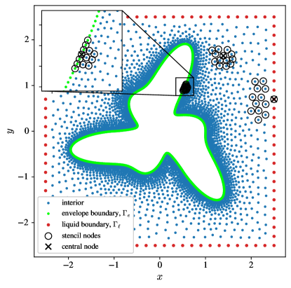
Figure 2: Example h-refined domain discretization. Additionally, example stencils on Dirichlet (green), Neumann (red) boundary and in the interior (blue) are shown.

To ensure an accurate description of the grain envelope and of the steep diffusion field in the vicinity of the envelope we employ h-refinement through the following internodal distance function

$$h(\boldsymbol{x})=\begin{cases}h_{\mathrm{e}}&,\text{ if }\boldsymbol{x}\in\Gamma_{\mathrm{e}}\\ h_{\ell}&,\text{ if }\boldsymbol{x}\in\Gamma_{\ell}\\ h_{\mathrm{e}}+(h_{\ell}-h_{\mathrm{e}})\frac{d(\boldsymbol{x})}{d_{\mathrm{closest}}}&,\text{ otherwise}\end{cases},$$ (8)

where $h_{\mathrm{e}}$ and $h_{\ell}$ are the internodal distances on the grain envelope and the outer liquid boundary, $d(\boldsymbol{x})$ is the Euclidean distance between $\boldsymbol{x}$ and the nearest node on the envelope, and $d_{\text{closest}}$ is the Euclidean distance between the node on the envelope boundary, $\Gamma_{\mathrm{e}}$, nearest to $\boldsymbol{x}$ and the node on the outer liquid boundary, $\Gamma_{\ell}$, nearest to $\boldsymbol{x}$. In our case, $h_{\mathrm{e}}<h_{\ell}$. Such definition of $h(\boldsymbol{x})$ gives a linearly decreasing internodal distance towards the envelope, as shown in Figure 2 with green coloured nodes on an illustrative dendrite-like shape.

4.2 Criterion for domain re-discretization

With the growth of the grain the envelope boundary moves and the shape and size of the domain therefore evolves. The spatial discretization must therefore be adapted with time. Besides the approximation of the differential operators, the domain discretization is among the most computationally demanding parts of Algorithm 1. Since the displacements of the envelope nodes within a single time step are typically small (much smaller than the local internodal distance $h_{\mathrm{e}}$) and since RBF-FD is relatively robust to non-optimal nodal positions [26, 21], it is not necessary to regenerate the discretization of the computational domain at each time step. Instead, we use a criterion based on the cumulative displacement magnitudes for each node $\boldsymbol{x}_{\mathrm{env}}$ on the envelope. The cumulative displacement magnitudes are collected in an array-like data type $\varphi$, which essentially holds information about the total displacement magnitude of all envelope nodes since the last domain re-discretization.

Based on the maximum cumulative displacement among all nodes, $\max(\varphi)$, we then distinguish between two possible cases (see line 16 in Algorithm 1):

$\max(\varphi)<h_{\mathrm{e}}/2:$

The largest cumulative displacement of the envelope node is smaller than half of the local internodal distance on the envelope, $h_{\mathrm{e}}$. Note that $h_{\mathrm{e}}$ is a parameter of the method and is constant. In this case re-discretization of the computational domain is not yet necessary. The envelope nodes are repositioned from $\Gamma_{\mathrm{e}}$ to $\Gamma_{\mathrm{e}}^{\star}$, according to the GEM. To avoid that computational nodes from the interior of the domain are too close to or inside the recomputed grain envelope (as this may affect the stability of the RBF-FD approximation), all nodes that fall inside the new envelope $\Gamma_{\mathrm{e}}^{\star}$ or are closer than $0.8h_{\mathrm{e}}$ to the envelope are removed from the domain $\Omega$.

$\max(\varphi)\geq h_{\mathrm{e}}/2:$

The largest cumulative displacement is larger or equal to half of the local internodal distance $h_{\mathrm{e}}$. In this case a complete re-discretization of the computational domain is required. The algorithm for re-discretization is given in Algorithm 2 in line 8 and gives the new computational nodes. The corresponding concentration field is obtained by mapping (interpolating) the field from the old to the new discretization (Algorithm 1, line 18). The interpolation method is discussed in detail in Section 4.4.1.

4.3 Meshless approximation of differential operators

The next step is the discretization of partial differential operators $\mathcal{L}$, in our case $\nabla^{2}$ and $\nabla$, which appear in Equation (4) and on the Neumann boundary, respectively. For each computational node $\boldsymbol{x}_{i}$ in the domain, a set of nearby nodes $\mathcal{N}_{i}=\left\{\boldsymbol{x}_{j}\right\}_{j=1}^{n}$, commonly called stencil or support nodes, is defined. While special stencil node selection algorithms showed promising results [27, 28], we use the simplest approach and choose the closest $n$ nodes according to the Euclidean distance, obtained efficiently by constructing a $k$-d tree. Example stencils in the interior of the domain and on the Dirichlet and Neumann boundaries are shown in Figure 2.

Once the stencil is defined, a linear differential operator $\mathcal{L}$ in node $\boldsymbol{x}_{c}$ is approximated over a set of $n$ stencil nodes $\mathcal{N}_{c}$ with

$$(\mathcal{L}u)(\boldsymbol{x}_{c})\approx\sum_{j=1}^{n}w_{j}u_{j}(\boldsymbol{x}_{j}),$$ (9)

for stencil nodes $\boldsymbol{x}_{j}\in\mathcal{N}_{c}$, function $u$ with nodal values $u_{j}$ and weights $\boldsymbol{w}$. The weights are obtained by solving a linear system, assembled from the chosen set of basis functions.

In this work, we use polyharmonic splines (PHS) [29] augmented with $N_{p}=\binom{m+d}{m}$ monomials up to order $m$ in the $d=2$ dimensional domain $\Omega$.

This corresponds to a commonly used meshless method, also referred to as the RBF-FD approximation [15, 30, 29].

By enforcing the equality of Equation (9) for the approximation basis, we can write a linear system

$$\underbrace{\begin{bmatrix}\boldsymbol{\Phi}&\boldsymbol{P}\\ \boldsymbol{P}^{\mathsf{T}}&\boldsymbol{0}\end{bmatrix}}_{\boldsymbol{A}}\begin{bmatrix}\boldsymbol{w}\\ \boldsymbol{\lambda}\end{bmatrix}=\begin{bmatrix}\boldsymbol{\ell}_{\phi}\\ \boldsymbol{\ell}_{p}\end{bmatrix},$$ (10)

with matrix $\boldsymbol{P}\in\mathbb{R}^{n\times N_{p}}$ of the evaluated monomials, matrix $\boldsymbol{\Phi}\in\mathbb{R}^{n\times n}$ of the evaluated RBFs and $\boldsymbol{\ell}_{\phi}$ and $\boldsymbol{\ell}_{p}$ are vectors of values assembled by applying the considered operator $\mathcal{L}$ to the RBFs and monomials respectively. To obtain the weights $\boldsymbol{w}$, the system is solved and Lagrangian multipliers $\boldsymbol{\lambda}$ are discarded.

Note that the positive definite RBFs alone ensure the positive definiteness of matrices $\boldsymbol{A}$, while consistency up to a certain order is achieved by adding monomials to the approximation basis [29]. Moreover, we follow the recommendations of Bayona [14] and define the stencil size $n$ as

$$n=2N_{p}=2\binom{m+d}{m}$$ (11)

to ensure a stable approximation.

The approximation (9) also holds for $\mathcal{L}\coloneqq 1$, effectively allowing us to use the same formulation for the approximation of field values at locations that do not correspond to the discretization points. This property will be used in Section 4.4.1, where we seek an accurate interpolation of the concentration field at the stagnant-film positions $\boldsymbol{x}^{\delta}$.

Note that the formulation of RBF-FD allows us to control the order of the interpolation through the order of the augmenting monomials [23, 29]. In this study, we will experiment with the second ($m=2$) and fourth ($m=4$) orders.

4.4 Propagation of the envelope – moving the boundary

At each time step, the new solute concentration field, $u$, is obtained by discretizing the diffusion Equation (4) with the meshless approximation and solving it explicitly using the forward Euler time-marching scheme (see line 8 of Algorithm 1). With the known concentration field, the envelope velocities are calculated by the GEM and the grain envelope is then propagated (line 9 of Algorithm 1). Recall that the envelope speed depends on the concentration $u_{\delta}$ at the stagnant-film and on the direction of the envelope normal (see Equations (1–3)). Accordingly, each envelope node, $\boldsymbol{x}_{i,\mathrm{env}}$, is propagated to a new position, $\boldsymbol{x}^{\prime}_{i,\mathrm{env}}$, by

$$\boldsymbol{x}^{\prime}_{i,\mathrm{env}}=\boldsymbol{x}_{i,\mathrm{env}}+\cos(\vartheta_{i})\,v(u_{\delta,i})\,\boldsymbol{n}_{i}\,\mathrm{d}t\,,\quad\forall\boldsymbol{x}_{i,\mathrm{env}}\in\Gamma_{\mathrm{e}},$$ (12)

where the speed $v$ is given by the GEM model (Equations (2–3)) as a function of $u_{\delta,i}$, which is the concentration at $\boldsymbol{x}_{\delta,i}=\boldsymbol{x}_{i,\mathrm{env}}+\delta\,\boldsymbol{n}_{i}$ and $\vartheta_{i}$ is the minimum angle between the envelope normal $\boldsymbol{n}_{i}$ and the 4 unit directional vectors, i.e., $\pm\boldsymbol{\widehat{e}}_{x}$ and $\pm\boldsymbol{\widehat{e}}_{y}$.

It follows that the numerical error in the shape of the grain envelope depends on the accuracy of the evaluation of the stagnant-film concentration, $u_{\delta}$, and of the normal direction, $\boldsymbol{n}_{i}$. These error sources are studied in the following subsections. $u_{\delta}$ is calculated by interpolation of the concentration field; the accuracy of different interpolation methods is discussed in Section 4.4.1. The normal, $\boldsymbol{n}$, is calculated from a parametric reconstruction of the envelope with splines. The same reconstruction is also used for the discretization of the envelope and allows us to ensure quasi-uniform internodal distances on the envelope and consequently to generate a robust spatial discretization of the domain. The envelope reconstruction is discussed in Section 4.4.2 along with the influence of the spline degree, a key parameter of the reconstruction.

4.4.1 Interpolation of the solute concentration field

In the GEM, the stagnant-film concentration, $u_{\delta}$, is required at any position $\boldsymbol{x}^{\delta}=\boldsymbol{x}_{\mathrm{env}}+\delta\boldsymbol{n}$ within the domain space $\Omega$. Since the concentration is only given at the discretization points $\boldsymbol{x}_{i}\in\Omega$, a suitable interpolation is required. We consider the following three interpolation methods:

Shepard’s interpolation,

also known as inverse distance weighing, where the interpolant is a weighted average over the neighborhood,

i.e., the $n$ points closest to $\boldsymbol{x}^{\delta}$, defined as

$$u(\boldsymbol{x}^{\delta})=\begin{cases}\dfrac{\sum_{i=1}^{n}\omega_{i}(\boldsymbol{x}^{\delta})u(\boldsymbol{x}_{i})}{\sum_{i=1}^{n}\omega_{i}(\boldsymbol{x}^{\delta})}&,\text{ if }d(\boldsymbol{x},\boldsymbol{x}_{i})\neq 0\text{ for all }i\\ u(\boldsymbol{x}_{i})&,\text{ if }d(\boldsymbol{x},\boldsymbol{x}_{i})=0\text{ for some }i\end{cases},$$ (13)

for weights $\omega_{i}(\boldsymbol{x}^{\delta})=\left\|\boldsymbol{x}^{\delta}-\boldsymbol{x}_{i}\right\|^{-\alpha}$ with power parameter $\alpha=2$.

The RBF-FD interpolation,

which uses the RBF-FD approximation described in Section 4.3 to build a local interpolant $F_{i}(\boldsymbol{x}^{\delta})$ over stencil nodes $\mathcal{N}(\boldsymbol{x}^{\delta})$ to obtain a local interpolation of the concentration in $\boldsymbol{x}^{\delta}$ for a chosen approximation basis.

The partition-of-unity (PU) interpolation,

which uses local RBF-FD interpolants and additionally constructs a global representation of the concentration field by employing the PU interpolation [31, 32]. Essentially, the PU approach builds local interpolants $F_{i}$ over stencil nodes $\mathcal{N}_{i}$ for all $N$ discretization nodes $\boldsymbol{x}_{i}\in\Omega$. The global interpolant is then constructed as

$$F(\boldsymbol{x})=\sum_{i=1}^{N}w_{i}(\boldsymbol{x})F_{i}(\boldsymbol{x}),$$ (14)

using compactly supported weights $w_{i}$ that form a partition-of-unity, $\sum_{i=1}^{N}w_{i}(\boldsymbol{x})=1$, for all $\boldsymbol{x}\in\Omega$. The most efficient way to construct the weights is to use the Shepard’s construction (see Equation 13) thus

$$w_{i}(\boldsymbol{x})=\frac{\omega(\left\|\boldsymbol{x}-\boldsymbol{x}_{i}\right\|/r_{i})}{\sum_{j=1}^{N}\omega(\left\|\boldsymbol{x}-\boldsymbol{x}_{j}\right\|/r_{j})},$$ (15)

where $r$ determines the effective radius of the individual interpolants $F$ – the larger the radius, the more pronounced the averaging effect. Such a construction effectively leads to a weighted average of the local interpolants $F_{i}$, where $\left\|\boldsymbol{x}_{i}-\boldsymbol{x}\right\|<r_{i}$, otherwise the weight is 0.

To evaluate the performance of the proposed interpolation methods, all three are further discussed and compared in terms of computational complexity and interpolation accuracy.

• Computational complexity
  The computational complexity of the three interpolation methods is anything but equivalent. Common to all is the construction of a $k$-d tree that allows us to query the nearest $n$ neighbours. Constructing such a structure for a domain with $N$ nodes requires $\mathcal{O}(N\log N)$ operations, while searching for $n$ nearest neighbours requires $\mathcal{O}(n\log N)$ operations.

  The evaluation of Shepard’s interpolant then requires additional $\mathcal{O}(n)$ operations. The construction of the RBF-FD interpolant requires $\mathcal{O}(n^{3})$ operations to solve the dense linear interpolation system from Equation (10) and additional $\mathcal{O}(n)$ operations to evaluate. The computational complexity of PU is generally higher than that of RBF-FD. In the worst case, i.e., with uniformly distributed nodes and a single query point, the construction of the PU interpolant requires $\mathcal{O}(n(n^{3}+n))$ operations. The first term comes from the construction of the RBF-FD interpolant and the second term comes from the calculation of Shepard’s weights. To evaluate the PU interpolant, further $\mathcal{O}(n)$ operations are required.

  Thus, the construction of the PU interpolant is the most computationally expensive, followed by the RBF-FD approximant and finally Shepard’s interpolant as the cheapest of the three.

• Interpolation accuracy
  The accuracy of each interpolation approach is evaluated using a two-dimensional Sibson’s function

  $$f(\boldsymbol{x})=f(x,y)=\cos(4\pi\sqrt{(x-1/4)^{2}+(y-1/4)^{2}})$$ (16)

  for the domain space $\boldsymbol{x}\in[0,1]^{2}$. We generate $N_{\mathrm{fit}}$ uniformly scattered fit points on which we construct the three proposed interpolation methods and we evaluate the accuracy of the interpolations on $N_{\mathrm{test}}\approx 10^{5}$ regularly positioned test nodes, ${\boldsymbol{x}}^{\prime}\in[0,1]^{2}$. The performance of the three interpolation methods is evaluated in Figure 3. On the left, we show the interpolated values using $N_{\mathrm{fit}}=384$ fitting points (marked with black crosses).

  In the center plot, we evaluate the relative error of all three interpolation methods as function of the neighbourhood/stencil size, $n$. For clarity, black dashed lines indicate the stencil sizes $n=12$, recommended by RBF-FD for a second-order method ($m=2$), and $n=30$, recommended for a fourth-order method ($m=4$) (see Equation (11)). We find that Shepard’s interpolation leads to interpolation errors that are almost an order of magnitude larger than the errors of RBF-FD and PU. Increasing the neighbourhood size, $n$, only worsens the accuracy of Shepard’s interpolation. RBF-FD and PU show comparable accuracy, both at second and fourth order, with the error decreasing with increasing spline order.

  Similar observations are made by a convergence analysis with respect to $N_{\mathrm{fit}}$ and with recommended stencil sizes $n$, shown in the right plot of Figure 3. The number of closest neighbours for Sheppard’s interpolation is set to $n=3$, as it yielded the highest accuracy in the centre plot. The black dashed lines and their slopes, $k$, show the observed order of convergence.

  Based on these analyses, we have chosen the RBF-FD approach, as it represents the best trade-off between accuracy and computational complexity. Furthermore this method is inherently present in the solution procedure, which is advantageous in two respects: (i) no additional approximation algorithms need to be implemented and (ii) the approximation error of the interpolated concentration is in the worst case of the same order of magnitude as the approximation of the partial differential operators involved [21].

  

  Figure 3: Analysis of interpolation performance on a two-dimensional Sibson’s function. The left figure illustrates the interpolated field together with the fitting points marked as black crosses. The center figure shows the interpolation error with respect to the stencil size, $n$, in terms of the relative $\ell_{2}$ norm. The stencil sizes $n=12$ and $n=30$, recommended for $m=2$ and $m=4$, respectively, are shown with dashed vertical lines. The right figure shows the error with respect to the number of fitting points using recommended stencil sizes and $n=3$ for Sheppard’s interpolation. The black dashed lines and their slopes, $k$, indicate the observed order of convergence.

4.4.2 Grain envelope reconstruction

The spatial propagation of the envelope nodes, as the grain grows, introduces two difficulties. First, the node spacing increases and the local internodal distance $h$ sooner or later violates the requirement of a quasi-uniform internodal distance for stable meshless approximations [33, 34, 16]. Second, some of the nodes from the interior of the computational domain are eventually engulfed by the growing envelope and thus fall outside the domain. Both problems lead to an unstable solution procedure and must therefore be handled accordingly.

To avoid such behaviour, the entire domain is re-discretized when necessary (see line 16 of Algorithm 1), according to the criterion introduced in Section 4.1. The first step of the re-discretization is a reconstruction of the envelope (see line 17 of Algorithm 1) using a generalised surface reconstruction algorithm [35]. This constructs a parametric representation of the envelope using splines $\gamma$ of the $k$-th degree over the translated nodes. Once the parametric representation of the envelope is obtained, a special surface DIVG algorithm [25] is used to populate it with a new set of nodes that are suitable for the RBF-FD approximation method [16].

The rest of the domain can then be discretized with the general DIVG node positioning algorithm.

Algorithm 2 Discretized boundary surface reconstruction.

Input: Envelope boundary nodes $\Gamma_{e}$, nodal density function $h:~{}\Omega\to\mathbb{R}$, parametric spline degree $k$.
Output: New domain discretization $\Omega^{\star}$.

1:function discretize_envelope($\Gamma_{\mathrm{e}},h,k$)

2:     $\sigma\leftarrow\textsc{order\_nodes}(\Gamma_{\mathrm{e}})$ $\triangleright$ Returns permutation of nodes $\sigma$.

3:     $\gamma\leftarrow\textsc{fit\_spline}(\Gamma_{\mathrm{e}},\sigma,k)$ $\triangleright$ Fits spline to ordered points.

4:     $\Gamma_{\mathrm{e}}^{\star}\leftarrow\textsc{discretize}(\gamma,h)$ $\triangleright$ Obtaines new envelope discretization.

5:     return $\Gamma_{\mathrm{e}}^{\star}$

6:end function

7:

8:function re-discretize_domain($\Gamma_{\mathrm{e}},h,k$)

9:     $\Gamma_{\mathrm{e}}^{\star}\leftarrow\textsc{discretize\_envelope}(\Gamma_{\mathrm{e}},h,k)$ $\triangleright$ Obtaines new envelope discretization.

10:     $\Omega^{\star}\leftarrow\textsc{discretize}(\Gamma_{\mathrm{e}}^{\star},h)$ $\triangleright$ Obtaines new domain discretization.

11:     return $\Omega^{\star}$

12:end function

The surface reconstruction is performed by Algorithm 2, which takes a set of randomly ordered envelope nodes $\Gamma_{\mathrm{e}}$ about to be parametrized with a Jordan curve $\gamma:[a,b]\rightarrow\mathbb{R}^{2}$. To obtain the Jordan curve, the nodes are first ordered, therefore, a $k$-d tree with envelope nodes is constructed, which allows us to query for nearest neighbours, obtaining a permutation array, $\sigma$, in the process. To find the appropriate permutation $\sigma$, the list of ordered points is first initialized with an arbitrary starting point $\boldsymbol{x}_{0}$. Its nearest neighbour $\boldsymbol{x}_{p}$ is then obtained using the $k$-d tree and added to the list of ordered points. The remaining nodes are then inductively ordered: Once $\boldsymbol{x}_{j}$ is in the list of ordered points, find its nearest neighbour $\boldsymbol{x}_{p}$. If $\boldsymbol{x}_{p}$ is not in the list of already ordered points, set $\boldsymbol{x}_{j+1}$ to $\boldsymbol{x}_{p}$, otherwise find the second (or $n$-th) nearest neighbour that is not yet in the list of ordered points. The process is repeated until all construction points from the envelope are ordered.

The ordered nodes are then used to re-construct the envelope shape by fitting a parametric spline $\gamma$ of $k$-th degree. $\gamma$ is discretized with a given point spacing as the new discretized grain envelope, $\Gamma_{\mathrm{e}}^{\star}$. For a graphical demonstration of the surface reconstruction algorithm, see Figure 4.

To discretize the rest of the domain (see line 10 of Algorithm 2), an inside check algorithm is required to distinguish between the interior and exterior of $\Gamma_{\mathrm{e}}^{\star}$. To determine whether a node $\boldsymbol{x}$ is inside $\Gamma_{\mathrm{e}}^{\star}$, a scalar product

$$\left\langle\boldsymbol{x}-\gamma(t_{\min}),c{\gamma}^{\prime\prime}(t_{\min})\right\rangle,$$ (17)

is computed. Here, $\gamma(t_{\min})$ is a node on the envelope closest to $\boldsymbol{x}$ and ${\gamma}^{\prime\prime}(t_{\min})$ is the normal vector in the same node. If the scalar product is negative, $\boldsymbol{x}$ is in the interior of $\Gamma_{\mathrm{e}}^{\star}$, otherwise not. The constant

$$c=-\mathrm{sgn}(\left\langle\boldsymbol{x}_{\mathrm{int}}-\gamma(t_{\min}),{\gamma}^{\prime\prime}(t_{\min})\right\rangle)$$ (18)

is computed for an arbitrary node $\boldsymbol{x}_{\mathrm{int}}$ from the interior and ensures that the normals point outwards. In Equation (18) $t_{\min}$ is determined so that the $\gamma(t_{\min})$ is closest to $\boldsymbol{x}_{\mathrm{int}}$.

Note: The reconstruction algorithm assumes the nodes from $\Gamma_{\mathrm{e}}$ must be dense enough to adequately describe the curve [35]. In our particular case of dendritic growth simulation we must choose a node spacing on and in the vicinity of the envelope, such that the internodal distance is much smaller than the radius of curvature of the envelope.

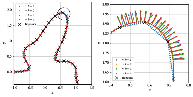
Figure 4: Example of surface reconstruction accompanied with normal vectors computed from the reconstructed spline $\gamma$ of degree $k\in\left\{1,2,3,4\right\}$. For clarity, the encircled area is zoomed in and shown on the right. We also show the normal directions in the right figure.

Choice of the spline degree for accurate envelope reconstruction

The effect of the spline degree is demonstrated in Figure 4 for degrees $k\in\left\{1,2,3,4\right\}$. As expected, a linear interpolation between two neighbouring nodes ($k=1$) does not yield a satisfying representation of the envelope.

Next, a more thorough discussion on the optimal spline degree $k$ for accurate surface reconstruction is given. The reconstruction quality is evaluated on a parametric function

$$R(t) =\lvert\cos(1.5t)\rvert^{\sin(3t)}$$ (19)

$$\boldsymbol{r}(t) =R(t)(\cos(t),\sin(t))$$ (20)

for values $t$ corresponding to the dendrite-tip-like shape (see Figure 5 left for clarity).

Figure 5: Parametric domain used to evaluate the accuracy of surface reconstruction (left) and reconstruction quality analysis (right) in terms of maximum radius error (top right) and maximum normal angle error (bottom right).

A set of equally spaced fit nodes is taken to obtain a parametric representation of the boundary. The internodal distance $h_{\mathrm{fit}}$ of fit points ranges from $0.1$ to $0.003$, resulting in $124$ and $4094$ fit points respectively. The test points, where the reconstruction quality is evaluated, are generated by discretizing the parametric representation of the boundary $\gamma$ with a uniform internodal distance $h_{\mathrm{test}}=0.005$, yielding approximately $2450$ test nodes.

The quality of the surface reconstruction is evaluated in terms of (i) the maximum error of the point position in terms of the distance $r=\sqrt{x^{2}+y^{2}}$ (top right in Figure 5) and (ii) the maximum error of the angle of the normal vector $\boldsymbol{n}\propto{\gamma}^{\prime\prime}(t)$ (bottom right in Figure 5); both within the domain of interest marked in light green in Figure 5 (left). From the analysis we conclude that the parametric representation of the envelope can be used to obtain an accurate reconstruction of the dendritic grain envelope, and that the spline degree $k$ significantly affects the accuracy of the reconstruction.

Note that a dashed vertical line has been added to the top and bottom right plots in Figure 5 to mark the internodal distance at which the density of the fit points is approximately equal to the density of the reconstructed nodes, i.e. $h_{\mathrm{fit}}\approx h_{\mathrm{test}}$. This is also mostly the case in the dendritic growth simulation governed by the GEM.

From the presented results, it is not possible to objectively deduce which spline degree $k$ yields a sufficiently accurate parametric representation of the dendritic grain envelope. The safest option is to choose the highest proposed spline degree, i.e. $k=4$, especially considering that the additional computational cost due to higher spline degrees is marginal.

A more systematic discussion is continued in Section 5, where the final decision on the spline degree $k=2$ used throughout the rest of this work is made.

4.5 Implementation remarks

The entire MIT solution procedure from Algorithm 1 using meshless methods is implemented in C++ environment. The projects implementation is strongly dependent on our in-house development of a meshless C++ Medusa library [36].

The code was compiled using g++ (GCC) 11.3.0 for Linux with -O3 -DNDEBUG flags on AMD EPYC 7702 64-Core Processor computer. OpenMP API has been used to run parts of the solution procedure in parallel on shared memory. Post-processing was done using Python 3.10.6 and Jupyter notebooks, also available in the provided git repository4.

5 MIT solution procedure verification: Isotropic growth of grain envelope

The goal of this section is analyse how the behaviour of the full MIT procedure depends (i) on the order of the RBF-FD approximation and (ii) on the order of the spline reconstruction of the envelope, and to quantify the errors linked to these methods.

To verify the full MIT solution procedure we propose a simple isotropic growth test, effectively forcing the Equation (12) to take the following form

$$\boldsymbol{x}_{i}^{\prime}=\boldsymbol{x}_{i}+v(u_{\delta,i})\boldsymbol{n}_{i}\mathrm{d}t,\quad\forall\boldsymbol{x}_{i}\in\Gamma_{\mathrm{e}},$$ (21)

and thus discarding the preferred directions of growth. With such setup, the grain envelope is expected to maintain its initial circular shape through all computational time steps and can therefore be used for verification of the method. The test is shown schematically in Figure 6(a). The computational domain is a circle of diameter $L=20$ with Neumann boundary conditions enforced on the outer (liquid) boundary $\Gamma_{\ell}$ and a Dirichlet boundary condition of $u=0$ enforced on the growing grain envelope $\Gamma_{\mathrm{e}}$. At time $t=0$, the envelope is initialized with a circle of radius $r_{0}=0.22239$ and the liquid in the domain $\Omega$ has a uniform initial concentration of $u_{0}=0.18$.

(a) Schematic representation of the isotropic problem. In the top right corner a set of black nodes is used to illustrate the h-refinement towards the envelope.

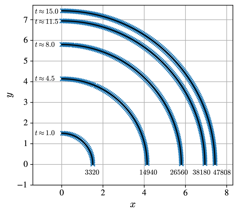
(b) Isotropic growth time lapse for 5 simulations times $t$ with the total number of time steps written at bottom of each envelope.

Figure 6: Presentation of the isotropic growth case.

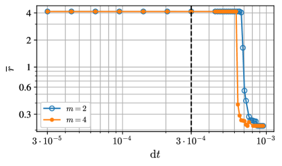
Figure 7: Average radius of the isotropic envelope at simulation time $t=4.5$ with respect to time step $\mathrm{d}t$.

In Figure 6(b), a time-lapse of the isotropic envelope calculated with MIT shows the circular envelope expansion. For clarity, a black line is constructed to demonstrate an exact circular shape, with the radius equal to the mean distance of the envelope nodes from the grain center.

Before we perform the analysis of MIT spatial discretization error, a scan over the time step size is performed to ensure an appropriate temporal discretization. In Figure 7, the average envelope radius $\overline{r}$ at simulation time $t=4.5$ is shown with respect to the time step $\mathrm{d}t$. Too large time steps ($\mathrm{d}t\geq 6\cdot 10^{-4}$) result in divergent solutions, while time steps $\mathrm{d}t\leq 3\cdot 10^{-4}$ give stable solutions for both the second and fourth order discretization approaches. Therefore, we use $dt=3\cdot 10^{-4}$ in all following discussions.

Next, Figure 8 shows the distortion of the calculated normal angle, $\vartheta(\boldsymbol{n})$, as function of the radial angle, $\vartheta(\boldsymbol{x}_{\mathrm{env}})$. The deviations from the ideal circular shape do not significantly depend on the spline degree, $k$, for $k>1$, while $k=1$ is too low for adequate surface reconstruction. We also observe a significant improvement in MIT accuracy when using a higher order RBF-FD (compare the left and right plots of Figure 8, corresponding to the second and fourth order RBF-FD approximation, respectively). The shape deviations are presented in a more quantitative manner in Table 1, where the extrema of the distortion in the envelope radius, from the mean radius, $\overline{r}$, and the largest distortions of the normal angles, $\vartheta(\boldsymbol{n})-\vartheta(\boldsymbol{x}_{\mathrm{env}})$, are tabulated.

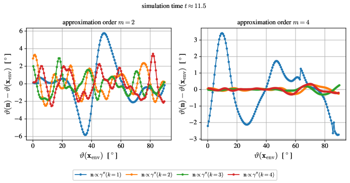
Figure 8: Shape distortion of the isotropic envelope: the difference in angle between the computed normal $\vartheta(\boldsymbol{n})$ and the angle of the radial vector pointed towards the envelope position $\vartheta(\boldsymbol{x}_{\rm env})$ at $t\approx 11.5$ using second order RBF-FD (left) and fourth order RBF-FD (right). $k$ is the order of the spline used for envelope reconstruction.

		$\overline{r}$	$\overline{r}-\min(r)$	$\max(r)-\overline{r}$	$\max(\vartheta(\boldsymbol{n})-\vartheta(\boldsymbol{x}_{\mathrm{env}}))$ [∘]	$\min(\vartheta(\boldsymbol{n})-\vartheta(\boldsymbol{x}_{\mathrm{env}}))$ [∘]
$m=2$	$\gamma(k=1)$	$7.3690$	$0.0340$	$0.0357$	$2.9411$	$-3.0012$
	$\gamma(k=2)$	$7.3967$	$0.0285$	$0.0203$	$3.9000$	$-4.0700$
	$\gamma(k=3)$	$7.3970$	$0.0225$	$0.0301$	$2.9738$	$-4.4241$
	$\gamma(k=4)$	$7.3983$	$0.0263$	$0.0238$	$2.8899$	$-3.0776$
	$\gamma(k=1)$	$7.3514$	$0.0322$	$0.0321$	$3.2313$	$-2.8206$
	$\gamma(k=2)$	$7.3913$	$0.0037$	$0.0031$	$0.3517$	$-0.2851$
	$\gamma(k=3)$	$7.3908$	$0.0036$	$0.0021$	$0.2039$	$-0.2423$
$m=4$	$\gamma(k=4)$	$7.3914$	$0.0014$	$0.0032$	$0.2227$	$-0.3810$

Table 1: Shape distortion from a circular shape at $t=11.5$ depending on the order of the RBF-FD approximation, $m$, and the on order of the splines for surface reconstruction, $k$. The distortion is represented in terms of the largest deviations from the mean radius, $r-\overline{r}$, and the largest distortions of the normal angles, $\vartheta(\boldsymbol{n})-\vartheta(\boldsymbol{x}_{\mathrm{env}})$.

From the above analysis we can conclude that: (i) splines of order $k>1$ should be used for envelope reconstruction to achieve good accuracy, (ii) shape distortions depend on the order of the RBF-FD and high-order ($m=4$) is required for high accuracy of the envelope normal direction, while the accuracy of the mean size (radius) is satisfactory even at low RBF-FD orders ($m=2$).

The temporal evolution of the two error metrics ($\vartheta(\boldsymbol{n})$ - $\vartheta(\boldsymbol{x}_{\rm env})$ and $\overline{r}\pm[\mathrm{min}(r),\mathrm{max}(r)]$) is assessed in Figure 9. Except for $k=1$ splines, the error strictly increases with time. It is now even more evident that $k=1$ does not give a sufficiently accurate surface reconstruction. The differences between the second- and fourth-order RBF-FD approximations are relatively small (less than 0.5% difference in the radius even at the end of the simulation), thus the use of the computationally much more demanding fourth-order method might not be justified.

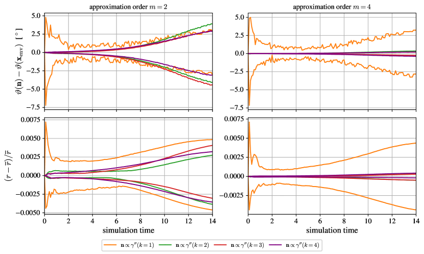
Figure 9: Time evolution of the shape distortion of the isotropic envelope. The top row shows distortion in normal vector angles and the bottom row shows distortion in terms of radius, the left column shows second order and the right column shows fourth order RBF-FD approximation.

6 Simulation of dendritic growth

Figure 10: Schematic representation of dendritic growth problem.

In this section we apply the MIT to the full GEM model to perform simulations of a dendritic grain and we compare the results to the PFIC method. The dendrite growth problem is schematically shown in Figure 10. The computational domain is a square of side length $L=20$ with Neumann boundary condition enforced on the outer (liquid) boundary $\Gamma_{\ell}$ and a Dirichlet boundary condition of $u=0$ enforced on the growing dendrite envelope $\Gamma_{\mathrm{e}}$. At time $t=0$, the dendrite envelope is initialized with a circle of radius $r_{0}=0.22239$ and the liquid in the domain $\Omega$ has a uniform initial concentration of $u_{0}=0.18$. The simulations are ran until the primary dendrite tip growing along the $x$ axis reaches position $x_{\text{tip}}=8.9$.

The node spacing on the envelope, $h_{\mathrm{e}}$ is kept constant throughout the simulation as described in Section 4.4.2. In the domain, the inner nodes are generated such that the node spacing increases linearly from $h_{\mathrm{e}}$ on the dendrite envelope to $h_{\ell}=0.1$ on the outer liquid boundary, according to the nodal density function defined in Equation (8). Note that $h_{\ell}=0.1$ is constant and identical for all simulations, regardless of $h_{\mathrm{e}}$. We use the RBF-FD approximation method, where the approximation basis consists of cubic PHS $r^{3}$ and monomials of second, $m=2$, and fourth, $m=4$, degree. In all cases, the differential operator approximation and the local interpolation of the concentration to the stagnant film are performed with the same RBF-FD setup. We present the results for both, i.e., the second and fourth order RBF approximations.

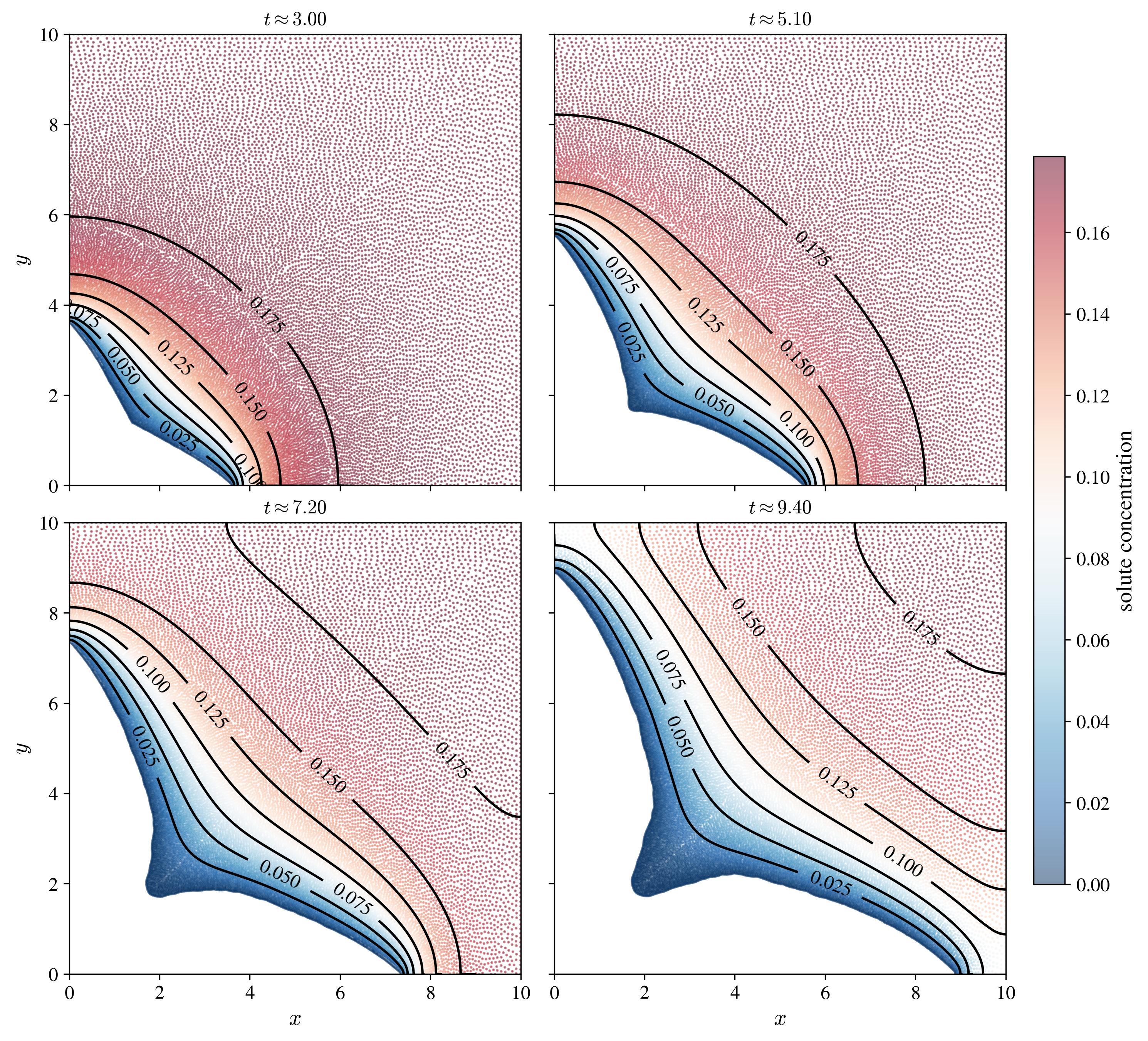
Figure 11: Growth of the dendritic grain envelope, the concentration field in the liquid and the adaptive discretization for $h_{\mathrm{e}}=0.028$

Figure 11 shows the solute concentration fields for selected simulation time steps computed with MIT using the internodal spacing $h_{\mathrm{e}}\approx 0.028$ on the dendrite envelope, effectively resulting in $67\,544$ and $77\,168$ discretization nodes at the first and last time steps, respectively. Note that due to the symmetry of the problem, only the first quadrant of the domain $\Omega$ is shown, although the entire dendrite was simulated.

To compare the MIT and PFIC methods, the envelope ($\Gamma_{\mathrm{e}}$) is compared at different times in Figure 12(a), along with the primary dendrite tip velocity with respect to time $t$ in Figure 12(b). Although the results of both methods are generally consistent and are very close, there are some differences that are the result of the differences of the two solution approaches. Nevertheless, the first remark can be made: Since PFIC and MIT generally agree, MIT can also be used to simulate GEM.

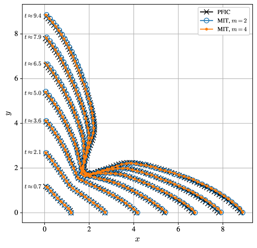
(a) Dendritic envelope shape time lapse.

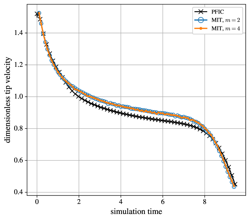
(b) Primary dendrite tip velocity with respect to simulation time.

Figure 12: Comparison of MIT and PFIC on dendritic growth problem for $h_{\mathrm{e}}\approx 0.028$.

Let us now take a closer look at the dendritic envelopes. To assess the behaviour of the numerical error in spatial discretization, we compare the envelopes computed with three different spatial discretizations at time $t\approx 9.6$, which corresponds to nearly the end of simulation time.

Figure 13 shows the results for the finest ($h_{\mathrm{e}}\approx 0.028$), intermediate ($h_{\mathrm{e}}\approx 0.060$), and coarsest ($h_{\mathrm{e}}\approx 0.1$) using the proposed MIT-based approach and the results for the finest ($h\approx 0.02$), intermediate ($h\approx 0.05$), and coarsest ($h\approx 0.1$) discretizations using the PFIC-based approach. Note that the mesh spacing, $h$, of the PFIC is uniform and equal to $h_{\mathrm{e}}$.

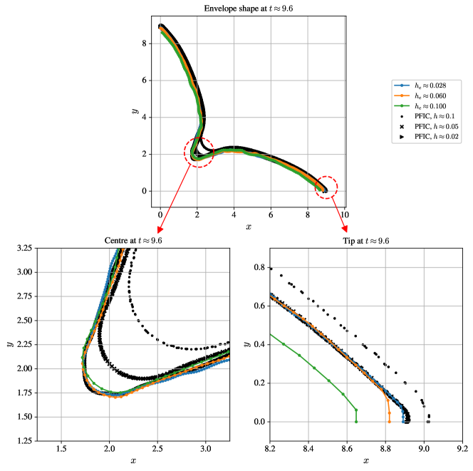
Figure 13: Convergence of the envelope shape at a selected simulation time $t\approx 9.6$. In the bottom row, the centre of the dendrite is shown on the left while the tip shape is shown on the right.

Convergent behaviour of the maximum tip position can be already seen in Figure 13 at the bottom right figure. To further support this observation, the maximum tip position is plotted with respect to the discretization spacing in Figure 14 (left) near the end of the simulation. Here we can see that the slope of convergence of the MIT-based approach is steeper than that of PFIC and also that MIT reaches the asymptotic value at somewhat larger node spacing than PFIC. The PFIC-based approach converges towards slightly larger tip positions than those obtained with the MIT-based simulation. Nevertheless, the difference between the two is less than 0.5 %, which is small, considering that we are comparing two conceptually different methods. We also show that increasing the order of the RBF approximation from second ($m=2$) to fourth ($m=4$) has only negligible impact on the solution of the full GEM.

In the middle of the dendrite (see Figure 13 in the lower left corner), we notice that MIT captures the final envelope shape with fewer nodes compared to PFIC. Note that PFIC with $h_{\mathrm{e}}\approx 0.1$ completely smooths out the depression in the centre, while MIT with a comparable spatial discretization captures all the details. The most likely reason for this is that MIT uses sharp interface tracking and avoids the smoothing effect of the phase field in curved parts of the shape, effectively requiring less nodes to reduce numerical artefacts. We attempt to evaluate this effect by measuring the length of the envelope. To do this, we use the spline representation of the dendritic envelope and calculate its total length by summing 5000 linear segments, which is shown in Figure 14 (right).

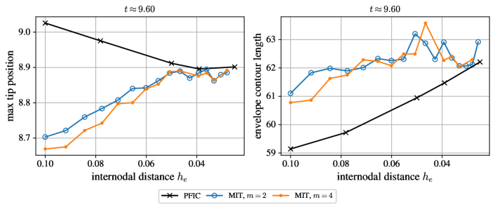
Figure 14: Maximum tip position with respect to the discretization spacing (left) and envelope contour length (right).

To show the benefit of h-adaptive discretization for the GEM we analyse the evolution of the number of discretization nodes during the simulations. Figure 15(a) shows the total number of nodes (domain and boundary nodes), $N_{\mathrm{total}}$, with respect to the internodal distance $h_{\mathrm{e}}$. The number of nodes is generally much lower with the MIT approach, because in the MIT (i) the interior of the dendrite is not considered as part of the computational domain, and (ii) the $h$-refinement towards the dendrite envelope effectively leads to a lower total number of nodes, while preserving the quality of the local field description near the envelope. The last two remarks are particularly important for fine internodal distances $h_{\mathrm{e}}$, which yield about an order of magnitude fewer computational points for the MIT at $h_{\mathrm{e}}\approx 0.028$. Figure 15(b) shows the evolution of the total number of discretization nodes with respect to the simulation time for the finest discretization used in this work ($h_{\mathrm{e}}\approx 0.028$). Given the h-refinement, we find that the number of discretization points generally increases during the simulation. This is somewhat intuitive since the dendrite area increases with simulation time, i.e., the densely populated area increases. On the other hand, an increasing size of the dendrite also means a decrease in the total domain size, which prevails as the dendrite envelope approaches the outer boundary of the domain.

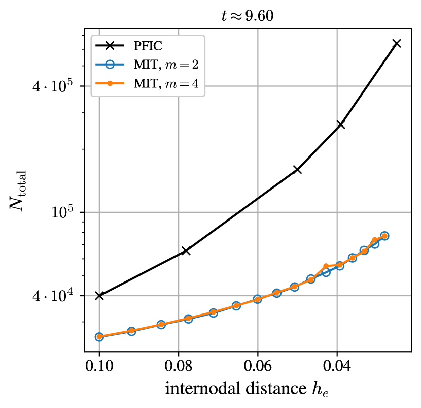
(a) Number of nodes at simulation time $t\approx 9.60$ with respect to the internodal distance $h_{\mathrm{e}}$, comparison of MIT and PFIC.

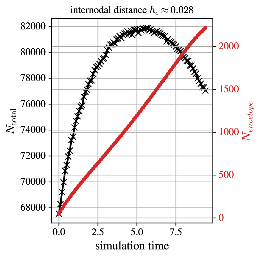
(b) Time evolution of the number of nodes for the MIT for $h_{\mathrm{e}}=0.028$.

Figure 15: Analysis of the number of discretization nodes for h-adaptive MIT and comparison to PFIC.

7 Conclusions and perspectives

In this paper we proposed the Meshless Interface Tracking (MIT) method for the solution of the Grain Envelope Model for dendritic growth (GEM). This novel method is expected to provide improved accuracy of GEM solutions in comparison with the Phase-Field Interface Capturing (PFIC) method, which has been used in all prior work on the GEM. Inherently, the MIT-GEM eliminates certain numerical artefacts experienced with the PFIC-GEM:

• The MIT-GEM does not smooth the envelope, while smoothing cannot be entirely avoided with the PFIC-GEM.

• The MIT-GEM ensures that the envelope propagates exactly at the calculated speed, while the PFIC-GEM requires a careful surface reconstruction to ensure good accuracy of the envelope propagation.

Furthermore, the MIT introduces h-adaptive spatial discretization, which is an advantage and enables one to ensure high accuracy of the solution of the diffusion field in the liquid. In the future it could also be used to refine the point spacing on the envelope in areas of high curvature.

We analysed all critical elements of the MIT method, namely the RBF approximation of the differential operators, the interpolation of the concentration field, and the parametric envelope reconstruction used for rediscretization and for calculation of the envelope speed. We addressed the accuracy and computational complexity of the methods as well as the sensitivity to the order of RBF operator approximation and to the order of spline interpolation for envelope reconstruction.

The comparison of PFIC and MIT shows that MIT can capture the shape of the envelope more accurately by using fewer nodes on the envelope. Moreover, due to the h-refinement, the total number of nodes required in MIT is also much smaller compared to PFIC. MIT reaches high accuracy using second order methods for the approximation of the spatial partial differential operators, spatial field interpolation, and for spline reconstruction of the envelope. Higher order methods can be readily used for additional improvement of accuracy.

The focus of future applications of the MIT-GEM will be simulations requiring high accuracy, especially high accuracy of the envelope tracking. This includes simulations where the development of new branches of a dendrite is a key aspect. The MIT-GEM will also serve as a high-accuracy reference for the verification of the computationally cheaper PFIC-GEM. From the numerical point of view, the introduction of a more complex node distribution that adapts to the local envelope curvature radius would be beneficial to improve the description of small-scale features of the envelope shape.

Declarations

Conflict of interest. The authors declare that they have no conflict of interest. All the co-authors have confirmed to know the submission of the manuscript by the corresponding author.

References

- [1] I. Steinbach, C. Beckermann, B. Kauerauf, Q. Li, J. Guo, Three-dimensional modeling of equiaxed dendritic growth on a mesoscopic scale, Acta Materialia 47 (1999) 971–982. doi:10.1016/S1359-6454(98)00380-2.
- [2] P. Delaleau, C. Beckermann, R. H. Mathiesen, L. Arnberg, Mesoscopic Simulation of Dendritic Growth Observed in X-ray Video Microscopy During Directional Solidification of Al–Cu Alloys, ISIJ International 50 (2010) 1886–1894. doi:10.2355/isijinternational.50.1886.
- [3] Y. Souhar, V. F. De Felice, C. Beckermann, H. Combeau, M. Založnik, Three-dimensional mesoscopic modeling of equiaxed dendritic solidification of a binary alloy, Computational Materials Science 112 (2016) 304–317.
- [4] I. Steinbach, H.-J. Diepers, C. Beckermann, Transient growth and interaction of equiaxed dendrites, Journal of crystal growth 275 (3-4) (2005) 624–638.
- [5] A. Olmedilla, M. Založnik, H. Combeau, Quantitative 3D mesoscopic modeling of grain interactions during equiaxed dendritic solidification in a thin sample, Acta Materialia 173 (2019) 249–261. doi:10.1016/j.actamat.2019.05.019.
-
[6]
A. Chirouf, B. Appolaire, A. Finel, Y. Le Bouar, M. Založnik,
Investigation of
diffusive grain interactions during equiaxed dendritic solidification, IOP
Conference Series: Materials Science and Engineering 1281 (2023) 012054.
doi:10.1088/1757-899X/1281/1/012054.
URL https://dx.doi.org/10.1088/1757-899X/1281/1/012054 - [7] A. Viardin, M. Založnik, Y. Souhar, M. Apel, H. Combeau, Mesoscopic modeling of spacing and grain selection in columnar dendritic solidification: Envelope versus phase-field model, Acta Materialia 122 (2017) 386–399. doi:10.1016/j.actamat.2016.10.004.
- [8] A. Viardin, Y. Souhar, M. Cisternas Fernández, M. Apel, M. Založnik, Mesoscopic modeling of equiaxed and columnar solidification microstructures under forced flow and buoyancy-driven flow in hypergravity: Envelope versus phase-field model, Acta Materialia 199 (2020) 680–694. doi:10.1016/j.actamat.2020.07.069.
- [9] M. Torabi Rad, M. Založnik, H. Combeau, C. Beckermann, Upscaling mesoscopic simulation results to develop constitutive relations for macroscopic modeling of equiaxed dendritic solidification, Materialia 5 (November 2018) (2019). doi:10.1016/j.mtla.2019.100231.
- [10] D. Tourret, L. Sturz, A. Viardin, M. Založnik, Comparing mesoscopic models for dendritic growth, in: IOP Conference Series: Materials Science and Engineering, Vol. 861, IOP Publishing, 2020, p. 012002.
-
[11]
A. K. Boukellal, M. Založnik, J.-M. Debierre,
Multi-scale
modeling of equiaxed dendritic solidification of al-cu at constant cooling
rate, IOP Conference Series: Materials Science and Engineering 1281 (2023)
012048.
doi:10.1088/1757-899X/1281/1/012048.
URL https://dx.doi.org/10.1088/1757-899X/1281/1/012048 - [12] Y. Sun, C. Beckermann, sharp-interface tracking using the phase-field equation, Journal of Computational Physics 220 (2) (2007) 626–653.
-
[13]
V. P. Nguyen, T. Rabczuk, S. Bordas, M. Duflot,
Meshless methods: a
review and computer implementation aspects, Math. Comput. Simul 79 (3)
(2008) 763–813.
doi:10.1016/j.matcom.2008.01.003.
URL https://sourceforge.net/projects/elemfregalerkin/ - [14] V. Bayona, An insight into rbf-fd approximations augmented with polynomials, Computers & Mathematics with Applications 77 (9) (2019) 2337–2353.
- [15] A. Tolstykh, D. Shirobokov, On using radial basis functions in a “finite difference mode” with applications to elasticity problems, Computational Mechanics 33 (1) (2003) 68–79.
- [16] J. Slak, G. Kosec, On generation of node distributions for meshless pde discretizations, SIAM journal on scientific computing 41 (5) (2019) A3202–A3229.
- [17] E. Ortega, E. Oñate, S. Idelsohn, R. Flores, A meshless finite point method for three-dimensional analysis of compressible flow problems involving moving boundaries and adaptivity, International Journal for Numerical Methods in Fluids 73 (4) (2013) 323–343, publisher: Wiley Online Library.
- [18] J. Slak, G. Kosec, Adaptive radial basis function–generated finite differences method for contact problems, International Journal for Numerical Methods in Engineering 119 (7) (2019) 661–686.
- [19] B. Cantor, A. Vogel, Dendritic solidification and fluid flow, Journal of Crystal Growth 41 (1) (1977) 109–123.
- [20] Y. Sun, C. Beckermann, A two-phase diffuse-interface model for Hele–Shaw flows with large property contrasts, Physica D: Nonlinear Phenomena 237 (2008) 3089–3098. doi:10.1016/j.physd.2008.06.010.
- [21] S. Le Borne, W. Leinen, Guidelines for rbf-fd discretization: Numerical experiments on the interplay of a multitude of parameter choices, Journal of Scientific Computing 95 (1) (2023) 8.
- [22] I. Tominec, E. Larsson, A. Heryudono, A least squares radial basis function finite difference method with improved stability properties, SIAM Journal on Scientific Computing 43 (2) (2021) A1441–A1471.
- [23] M. Jančič, J. Slak, G. Kosec, Monomial Augmentation Guidelines for RBF-FD from Accuracy Versus Computational Time Perspective, Journal of Scientific Computing 87 (1), publisher: Springer Science and Business Media LLC (Feb. 2021). doi:10.1007/s10915-020-01401-y.
-
[24]
M. Depolli, J. Slak, G. Kosec,
Parallel
domain discretization algorithm for RBF-FD and other meshless numerical
methods for solving PDEs, Computers & Structures 264 (2022) 106773.
doi:10.1016/j.compstruc.2022.106773.
URL https://linkinghub.elsevier.com/retrieve/pii/S0045794922000335 - [25] S. De Marchi, A. Martínez, E. Perracchione, Fast and stable rational rbf-based partition of unity interpolation, Journal of Computational and Applied Mathematics 349 (2019) 331–343.
- [26] M. Jančič, G. Kosec, Stability analysis of rbf-fd and wls based local strong form meshless methods on scattered nodes, in: 2022 45th Jubilee International Convention on Information, Communication and Electronic Technology (MIPRO), 2022, pp. 275–280. doi:10.23919/MIPRO55190.2022.9803334.
- [27] O. Davydov, D. T. Oanh, N. M. Tuong, Improved stencil selection for meshless finite difference methods in 3d, Journal of Computational and Applied Mathematics (2023) 115031.
- [28] M. Rot, A. Rashkovska, Meshless method stencil evaluation with machine learning, in: 2022 45th Jubilee International Convention on Information, Communication and Electronic Technology (MIPRO), 2022, pp. 269–274. doi:10.23919/MIPRO55190.2022.9803651.
- [29] V. Bayona, N. Flyer, B. Fornberg, G. A. Barnett, On the role of polynomials in rbf-fd approximations: Ii. numerical solution of elliptic pdes, Journal of Computational Physics 332 (2017) 257–273.
- [30] N. Flyer, B. Fornberg, V. Bayona, G. A. Barnett, On the role of polynomials in rbf-fd approximations: I. interpolation and accuracy, Journal of Computational Physics 321 (2016) 21–38.
- [31] J. Slak, Partition-of-unity based error indicator for local collocation meshless methods, in: 2021 44th International Convention on Information, Communication and Electronic Technology (MIPRO), 2021, pp. 254–258. doi:10.23919/MIPRO52101.2021.9597066.
-
[32]
S. De Marchi, A. Martínez, E. Perracchione,
Fast
and stable rational rbf-based partition of unity interpolation, Journal of
Computational and Applied Mathematics 349 (2019) 331–343.
doi:https://doi.org/10.1016/j.cam.2018.07.020.
URL https://www.sciencedirect.com/science/article/pii/S0377042718304400 - [33] H. Wendland, Scattered data approximation, Vol. 17, Cambridge university press, 2004.
- [34] V. Bayona, M. Moscoso, M. Carretero, M. Kindelan, Rbf-fd formulas and convergence properties, Journal of Computational Physics 229 (22) (2010) 8281–8295.
- [35] M. Jančič, V. Cvrtila, G. Kosec, Discretized boundary surface reconstruction, in: 2021 44th International Convention on Information, Communication and Electronic Technology (MIPRO), 2021, pp. 278–283. doi:10.23919/MIPRO52101.2021.9596965.
- [36] J. Slak, G. Kosec, Medusa: A c++ library for solving pdes using strong form mesh-free methods, ACM Transactions on Mathematical Software (TOMS) 47 (3) (2021) 1–25.