Regularization and Model Selection for Item-on-Items Regression with Applications to Food Products’ Survey Data

Abstract

Ordinal data are quite common in applied statistics. Although some model selection and regularization techniques for categorical predictors and ordinal response models have been developed over the past few years, less work has been done concerning ordinal-on-ordinal regression. Motivated by survey datasets on food products consisting of Likert-type items, we propose a strategy for smoothing and selection of ordinally scaled predictors in the cumulative logit model. First, the original group lasso is modified by use of difference penalties on neighbouring dummy coefficients, thus taking into account the predictors’ ordinal structure. Second, a fused lasso type penalty is presented for fusion of predictor categories and factor selection. The performance of both approaches is evaluated in simulation studies, while our primary case study is a survey on the willingness to pay for luxury food products.

Keywords: Cumulative Logit; Group Lasso; Likert-Scale; Luxury Food; Proprtional Odds Model; Sensometrics

1 Introduction

Ordinal categorical variables arise commonly in regression modeling. Still, proper treatment of the underlying scale level and appropriate statistical modeling is an issue of discussion. In many applications, the nature of ordinal predictors such as rating scales is neglected and a classical linear model is fit instead, thus assuming a metric scale level. At the other extreme, textbooks often transform ordinal covariates into dummy variables, thus using the variables’ nominal scale level only. Ignoring that categories are ordered implies, however, that we do not make full use of all the information contained in the data. If we now go one step further, many applications are found in the literature where the response variable is also ordinally scaled. If only the dependent variable is ordinal, ordered response models are typically used, which are treated in most advanced textbooks on statistical modeling. Although the analysis of ordinal response variables has been well investigated, ordinal-on-ordinal regression is hardly mentioned. Furthermore, regularization techniques already exist for both ordinal response models and ordinal predictors, but not for both together. The objective of the present paper is to close this gap and to offer methods for variable selection in the ordinal-on-ordinal setting. One such setting is a survey on luxury food (Hartmann et al., 2016, 2017), which will be the primary case study here. In this survey, data was collected on a variety of items measured on a 5-point Likert-type scale. The primary goal of the original study was to segment German consumers based on their perceived dimensions of luxury food and the shift of consumer consumption motives toward indulgence, quality, and sustainability. In what follows, we will focus on a regression problem where the response variable is the willingness to pay for luxury food products, which is evaluated on an ordinal 5-point scale as well. The set of predictors considered contains 43 ordinally scaled statements (items) on eating habits, shopping places/habits, the importance of price, eating style, and the subjective definition of luxury food.

High-dimensional surveys like this, with ordinal data both on the left and right-hand side of the regression, highlight the importance of regularization and variable selection in ordinal regression such as the cumulative logit model, because the full model is often hard to fit by ordinary/unpenalized maximum likelihood, and not all of the items available will be relevant for the response. Our aim is to investigate the effect of the ordinal covariates on the ordinal response while integrating strategies for variable selection and smoothing across covariate levels.

Various regularization techniques have been proposed for regression models in the last two decades. Based on the group lasso penalty (Yuan and Lin, 2006), factor selection in the logistic model has been done by Meier et al. (2008). Tutz and Gertheiss (2014, 2016) proposed methods for the selection of ordinally scaled independent variables in the classical linear, the logistic, and the log-linear (Poisson) model. Regularized ordinal regression has been considered for nominal or numerical covariates using an elastic net penalty by Wurm et al. (2021).

The limitation of the penalty approaches above, however, is that they assume either the response or the predictors to be of nominal or metric scale. We propose a strategy for model selection of ordinally scaled predictors in the cumulative logit model. The original group lasso is modified by the use of a difference penalty on neighbouring dummy coefficients, thus taking into account their ordinal structure. The main references for the cumulative logit model as described in the presented article are Fahrmeir and Tutz (2001) and Fahrmeir et al. (2013); a well-known introduction is found in Agresti (2002).

The remainder of the paper is organized as follows. Section 2 introduces two motivating data examples on food products and the corresponding modeling framework. In Section 3 we will present two penalty methods for ordinal predictors. Some illustrative simulation studies in Section 4 examine the quality of the proposed methodology. In Section 5 the proposed methods are applied to the study on luxury food expenditure. In Section 6 we conclude with a discussion. All computations were done using the statistical program R (R Core Team, 2021). The proposed method is implemented in the open-source R add-on package ordPens. The current package version is available on GitHub (https://github.com/ahoshiyar/ordPens) and will be soon accessible on CRAN as well.

2 Data Examples and Modeling Framework

2.1 Two Case Studies

2.1.1 Sustainable Use of Boar-Tainted Meat

For illustrative purposes, we first investigate a survey concerning consumers’ perception and acceptance of boiled sausages from strongly boar-tainted meat, conducted by the Department of Animal Sciences, University of Göttingen (Meier-Dinkel et al., 2016). Due to the European call for alternatives to surgical castration of male piglets, as this practice was proven to be cruel (European Commission, 2010, 2019), there is raising interest in the production and processing of boar meat. However, there is a disadvantageous risk that off-flavours occur, so-called boar taint, which is to be dealt with. An effort is being put into improving the processing of tainted raw material in a sustainable way with the primary aim of making it ‘fit for human consumption’. Specifically, one challenge lies in masking the undesirable odour –and the associated flavour– by combining spices/herbs/aromas and developing meat products that are palatable and accepted by consumers. The study at hand examined six sausages of different types (raw smoked-fermented or boiled emulsion-type sausages) with a varying proportion of tainted raw material ($50\%$, $100\%$, control product without tainted material). 120 participants were recruited to consume and evaluate the products with regard to different features. For illustrational purposes, we focus on boiled sausages here with a proportion of $50\%$ tainted boar meat (product $6$). In order to be able to process highly tainted meat sustainably, we aim to detect the relevant factors for the overall liking of the consumers regarding the sausages. The six ordinal predictors considered (expected liking, appear, odour, flavour, texture, aftertaste) and the ordinal response (overall liking) are measured on a $9$-point scale ($1=\text{dislike extremely}$ to $9=\text{like extremely}$). The data is summarized through barplots in Figure 1. Now, the effect of the ordinal covariates on the ordinal factor overall liking is to be investigated.

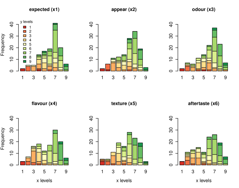
Figure 1: Illustration of the sensory data.

2.1.2 Spending on Luxury Food

As a second and main case study, we consider the before-mentioned survey concerning, among other things, the consumer’s willingness to pay for “luxury food”  (Hartmann et al., 2016, 2017). The part of the dataset we examine consists of 821 observations of 44 Likert-type items on personal luxury food definitions, eating and shopping habits, diet styles, and food price sensitivities. One such item is, for example, “I associate a high price in food with particularly good quality”, with coding scheme $-2=$ ‘strongly disagree’, $\ldots\,$, $+2=$ ‘fully agree’. The coding scheme of the remaining items is similar and given in Table S1 in Appendix C. Our response of interest is whether participants would be willing to pay a higher price for a food product that they associate with luxury, measured again on the ordinal $-2$ to $+2$ scale. The subset of the data that is analyzed here has been made publicly available at https://zenodo.org/record/8383248 (Hoshiyar et al., 2023). A different subset of the data has previously been studied by Tutz and Gertheiss (2016), but their focus was on aspects regarding more general behaviour when buying and consuming food products. Also, their response of interest was different, namely the (approximate) household’s weekly expenditure on food, measured on a metric scale.

2.2 Item-on-Items Regression

The cumulative model is probably the most popular regression model for dependent, ordinal variables. It can be motivated such that the observable response variable $Y\in\{1,\ldots,c\}$ is a categorized version of a latent continuous variable $u$. As usual in multivariate statistics, we assume that the predictor matrix $\boldsymbol{X}$ has entries $(\boldsymbol{X})_{ij}=x_{ij}$ denoting the value of the $j$th explanatory variable observed at the $i$th subject, $j=1,\ldots,p,i=1,\ldots,n$. The link between the response variable $Y_{i}$ (i.e., $Y$ for subject $i$) and the corresponding latent variable $u_{i}$ is then defined by the threshold mechanism

$$Y_{i}=r\Longleftrightarrow\theta_{r-1}<u_{i}\leq\theta_{r},\quad r=1,\ldots,c,$$

where $-\infty=\theta_{0}<\theta_{1}<\ldots<\theta_{c}=\infty$ are the ordered thresholds. The latent variable is typically modeled as

$$u_{i}=-\boldsymbol{x}^{\top}_{i}\boldsymbol{\beta}+\epsilon_{i},$$

where $\boldsymbol{x}_{i}=(x_{i1},\ldots,x_{ip})^{\top}$, $\boldsymbol{\beta}=(\beta_{1},\ldots,\beta_{p})^{\top}$ is the parameter vector and $\epsilon_{i}$ is an error variable with distribution function $F$. From these assumptions, it follows that

$$P(Y_{i}\leq r)=P(u_{i}\leq\theta_{r})=F(\theta_{r}+\boldsymbol{x}^{\top}_{i}\boldsymbol{\beta}),$$

or, equivalently,

$$P(Y_{i}=r)=\pi_{ir}=F(\eta_{ir})-F(\eta_{i,r-1}),\quad r=2,\ldots,c,$$

with $\eta_{ir}=\theta_{r}+\boldsymbol{x}^{\top}_{i}\boldsymbol{\beta}$ being the linear predictor and $P(Y_{i}=1)=\pi_{i1}=F(\eta_{i,1})$. Common choices for $F(\cdot)$ are the logistic and the standard normal cumulative distribution function, resulting in the cumulative logit and the cumulative probit model, respectively. The most widely used cumulative model is the cumulative logit model (cf. Tutz, 2022), which we will concentrate on here. The cumulative logit model is also known as the proportional odds model (POM) since the ratio of the cumulative odds for two populations is postulated to be the same across all categories.

Now, given the logistic distribution function $F(\eta_{ir})=1/(1+\exp(-\eta_{ir}))$, the cumulative logit model has the form

$$P(Y_{i}\leq r)=\frac{\exp(\theta_{r}+\boldsymbol{x}^{\top}_{i}\boldsymbol{\beta})}{1+\exp(\theta_{r}+\boldsymbol{x}^{\top}_{i}\boldsymbol{\beta})}.$$ (1)

Let $(y_{i1},\ldots,y_{ic})$ be binary indicators of the response for subject $i$, with $y_{ir}=1$ if $Y_{i}=r$ and zero otherwise. The log-likelihood for the sample is then given by

$$l(\boldsymbol{\theta},\boldsymbol{\beta})=\sum_{i=1}^{n}\sum_{r=1}^{c}y_{ir}\log{\pi_{ir}},$$ (2)

with

$$\pi_{ir}=\left\{\begin{array}[]{ll}\frac{\exp{(\eta_{ir})}}{1+\exp{(\eta_{ir})}},&r=1\\ \frac{\exp{(\eta_{ir})}}{1+\exp{(\eta_{ir})}}-\frac{\exp{(\eta_{i,r-1})}}{1+\exp{(\eta_{i,r-1})}},&r=2,\ldots,c\end{array}\right..$$

Estimation of unknown coefficients and ‘intercepts’ $\theta_{r}$ relies on well-known maximum likelihood principles. Further details can be found in Appendix A and in Fahrmeir and Tutz (2001).

With ordinal covariates, without loss of generality, matrix $\boldsymbol{X}$ contains integers $1,2,\ldots$, with entry $x_{ij}$ indicating the level of the $j$th variable that is observed at the $i$th subject. So let $\boldsymbol{x}_{j}$ have (potential) values $\boldsymbol{x}_{j}\in\{1,\ldots,k_{j}\}$ and define dummy variables such that $\boldsymbol{z}_{jl}=1$ if $\boldsymbol{x}_{j}=l$, $l=1,\ldots,k_{j}$, and $\boldsymbol{z}_{jl}=0$ otherwise. The complete indicator matrix is then given by $\boldsymbol{Z}=(\boldsymbol{Z}_{1}|\ldots|\boldsymbol{Z}_{p})$ and

$$\boldsymbol{Z}_{j}=(z_{ijl})=\begin{pmatrix}z_{1j1}&\cdots&z_{1jk_{j}}\\ \vdots&\ddots&\vdots\\ z_{nj1}&\cdots&z_{njk_{j}}\\ \end{pmatrix}.$$

The model to be fitted has the linear predictor

$$\eta_{ir}=\theta_{r}+\sum_{j=1}^{p}\sum_{l=1}^{k_{j}}z_{ijl}\beta_{jl}=\theta_{r}+\sum_{j=1}^{p}\boldsymbol{z}_{ij}^{\top}\boldsymbol{\beta}_{j},$$ (3)

where vector $\boldsymbol{\beta}_{j}$ contains all parameters linked to predictor $\boldsymbol{x}_{j}$. For reasons of identifiability, however, some restrictions are needed. For instance, by specifying a so-called reference category, e.g., category $1$ for each categorical covariate $\boldsymbol{x}_{j}$, and omitting the dummy variable for the first category, i.e., $\beta_{j1}=0\ \forall j$. Alternatively, one may set $\sum_{l}\beta_{jl}=0\ \forall j$, which is also known as ‘effect coding’. With respect to parameter estimates, all restrictions are equivalent. Consequently, the total number of parameters to be estimated is $(c-1)+\sum_{j=1}^{p}(k_{j}-1)$, as we have $c-1$ unknown thresholds and $k_{j}-1$ degrees of freedom for predictor $\boldsymbol{x}_{j}$.

For illustration, Figure 2 gives the estimated dummy coefficients in the proportional odds model when fit to the sensory data from Section 2.1.1 using the MASS::polr function in R (Venables and Ripley, 2002). In the first attempt to estimate the model, however, the algorithm did not converge. The function failed at finding suitable starting values.

This is a known problem with the function polr, since it estimates a (binary) logit model to initiate, and the function terminates when the GLM does not converge. Convergence problems occur when the fitted probabilities are extremely close to zero or one, as also addressed by Venables and Ripley (2002, p.197-198). However, fitting was possible when inserting some group lasso penalized estimates as starting values (compare Section 3). It is seen that polr estimates are very wiggly and thus hard to interpret. Moreover, some effects appear to be extremely large (note, the effects refer to the logit scale here), causing some fitted response probabilities to be numerically zero or one. The reason for that becomes clear when looking at the data in Figure 1. Typically, there is only a small number of samples found in the lowest x-category (‘1’), with most (or even all) observations falling in the same and most extreme y-category ‘1’, whereas y-level ‘1’ is hardly found for x-levels greater than 1. As a consequence, fitting by pure maximum likelihood leads to (seemingly) extreme effects.

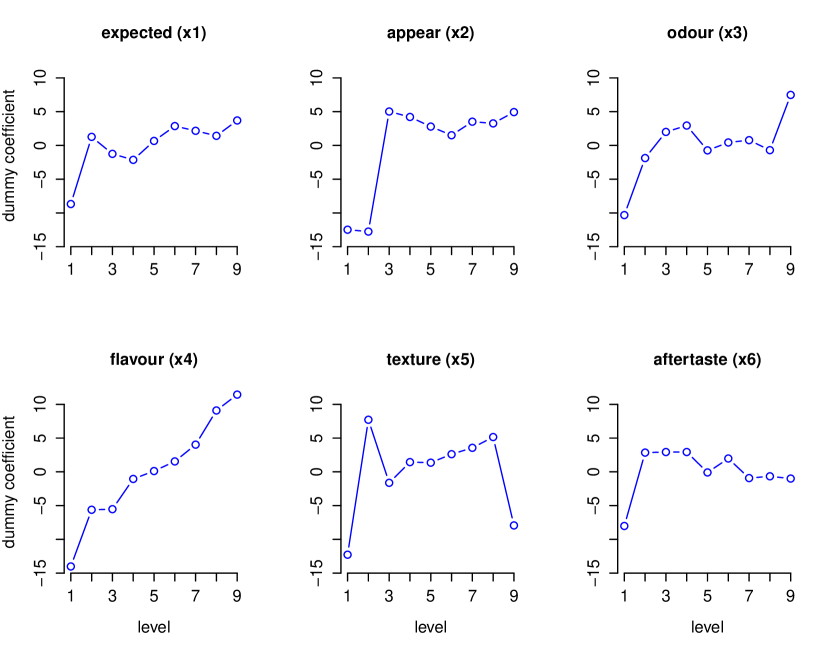
Figure 2: polr estimates of effect coded coefficients as functions of class labels for the sensory data from Section 2.1.1. The estimated thresholds/intercepts are: $-34.22,-1.20,4.84,7.32,8.86,11.29,15.75,21.98$.

3 Regularization and Model Selection

3.1 Groupwise Selection and Smoothing

With categorical predictors included in the model, resulting in a large (potentially enormous) number of parameters to be estimated, typically two challenges arise. The first is making a decision about the variables to include in the regression model. Secondly, we have to decide which categories within one categorical predictor should be distinguished. Furthermore, when $l(\boldsymbol{\theta},\boldsymbol{\beta})$ using (3) is maximized, only the nominal scale level of the predictor variables is used. As already discussed by Tutz and Gertheiss (2014, 2016) for other types of regression models, it can be beneficial to use special penalties to incorporate the predictors’ ordinal scale level. In particular, penalizing differences between adjacent coefficients as done by Gertheiss et al. (2011) seems promising. Analogously, the logistic group lasso estimator $\boldsymbol{\beta}_{\lambda}$ (Meier et al., 2008; Yuan and Lin, 2006) can be extended to the class of cumulative logit models and is given by the minimizer of the function

$$l_{\lambda}(\boldsymbol{\theta},\boldsymbol{\beta})=-\frac{1}{n}l(\boldsymbol{\theta},\boldsymbol{\beta})+\lambda\sum_{j=1}^{p}J_{j}(\boldsymbol{\beta}_{j}),$$ (4)

where $l(\boldsymbol{\theta},\boldsymbol{\beta})$ is the log-likelihood of the cumulative logistic distribution in (2). In order to take into account the ordinal structure of the predictors, we additionally modify the usual $L_{2}$-norm by the first-order difference penalty functions

$$J_{j}(\boldsymbol{\beta}_{j})=\sqrt{\Bigg{\{}\sum_{l=2}^{k_{j}}\text{df}_{j}(\beta_{jl}-\beta_{j,l-1})^{2}\Bigg{\}}}=\sqrt{\text{df}_{j}}||\boldsymbol{D}_{1,j}\boldsymbol{\beta}_{j}||_{2},$$ (5)

with $k_{j}$ being the number of levels (for each variable) and $\text{df}_{j}=k_{j}-1$. $||\cdot||_{2}$ denotes the $L_{2}$-norm and $((k_{j}-1)\times k_{j})$ matrix

$$\boldsymbol{D}_{1,j}=\begin{pmatrix}-1&1&&&\\ &-1&1&&\\ &&\ddots&\ddots&\\ &&&-1&1\\ \end{pmatrix}$$ (6)

generates differences of first order from the parameters linked to the $j$th predictor. This first-order penalty enforces selection of the whole group of parameters that belong to the same categorical predictor $\boldsymbol{x}_{j}$ and simultaneously smoothes over the ordered categories.

For finding the final solution, we can utilize the block co-ordinate gradient descent method of Tseng and Yun (2009), as described in Meier et al. (2008). Namely, combining a quadratic approximation of the log-likelihood with an additional line search. Based on the co-ordinate descent algorithm, the R package grplasso (Meier, 2020) provides (nominal) group lasso estimation for the Poisson, the logistic, and the classical linear model. For penalized item-on-item regression in terms of a cumulative logit model with ordinal predictors and corresponding ordinal smoothing penalty (5) some modifications have to be made. The modified method is described in detail in Appendix B.

The strength of penalization is controlled by parameter $\lambda$. With $\lambda=0$, unpenalized maximum likelihood estimates for categorical variables as described in Section 2.2 are obtained. If $\lambda\to\infty$ one obtains the extreme case that coefficients that belong to the same predictor are estimated to be equal, which means that the corresponding predictor has no effect on the response. In fact, with any of the restrictions (reference category set to zero, or, effect coding), all parameters except for intercepts/thresholds are estimated to be zero if $\lambda\to\infty$. Further note that penalized estimates as proposed here are invariant against the concrete choice of the restrictions, because the values of both the likelihood and penalty at (5) do not depend on the restriction chosen. Note that we do not penalize intercepts/thresholds $\theta_{r}$.

For illustration, we consider the example from Section 2.1.1. Figure 3 shows the resulting parameter estimates for the six covariates and different values of tuning parameter $\lambda$ when applying the proposed method to the boar-taint data. It is seen that for smaller $\lambda$ (light gray), the estimates are more wiggly (and more extreme) and become more and more smoothed out/shrunken as $\lambda$ increases. It is also seen that, at some point, the entire group of dummy coefficients belonging to one variable is set to zero, which means that the corresponding variable is excluded from the model. In general, the overall liking increases with the liking level of the covariates, with flavour apparently having the largest effect.

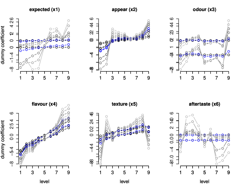
Figure 3: Cumulative group lasso estimates of effect coded coefficients as functions of class labels ($\lambda\in\{10,5,1,0.5,0.25\}/n$).

3.2 Ordinal-on-Ordinal Fusion

If a variable is selected by the smoothed group lasso (5), all coefficients belonging to that selected covariate are estimated as differing (at least slightly). However, it might be useful to collapse certain categories. Fusion of dummy coefficients of ordinal predictors has already been discussed for binary, numerical, and count response models by Tutz and Gertheiss (2014, 2016). We extend their previous work to the framework of the cumulative logit model. Clustering is done by a fused lasso-type penalty (Tibshirani et al., 2005) using the $L_{1}$-norm on adjacent categories. That is, adjacent categories may end up with exactly the same coefficient values and one obtains clusters of categories. The idea is to maximize $l_{\lambda}(\boldsymbol{\theta},\boldsymbol{\beta})$ at (2) with

$$J_{j}(\boldsymbol{\beta}_{j})=\sum_{l=2}^{k_{j}}|\beta_{jl}-\beta_{j,l-1}|.$$ (7)

Using the $L_{1}$-norm for neighbouring categories encourages that adjacent parameters are set exactly equal rather than just being close (as done by penalty (5)). Penalty (7) thus has the effect that neighbouring categories may be fused (namely, if they have the same $\boldsymbol{\beta}$ values). The fused lasso also enables selection of predictors: a predictor is excluded if all its categories are combined into one cluster. As already pointed out in Section 3.1 above, any of the restrictions considered here then effects that all parameters belonging to the respective predictor are set to zero. As before, penalty (7) is invariant against the concrete choice of restriction.

For computation, we make use of ordinalNet:ordinalNet() (Wurm et al., 2021), a function that provides ordinal regression models with elastic net penalty. If the elastic mixing parameter $\alpha\in[0,1]$ is set to alpha=1, the usual $L_{1}$ lasso penalty is applied. By appropriate recoding of the parameters and the design as proposed by Walter et al. (1987), the problem can be written as a problem in which the classical lasso penalty is used. The general split-coding scheme is as follows. The transformed design matrix becomes $\boldsymbol{\tilde{X}}=(\tilde{\boldsymbol{X}_{1}}|\ldots|\tilde{\boldsymbol{X}}_{p})$, $\tilde{\boldsymbol{\beta}}=(\tilde{\boldsymbol{\beta}}_{1}^{\top},\ldots,\tilde{\boldsymbol{\beta}}_{p}^{\top})^{\top}$ and $\tilde{\boldsymbol{X}}_{j}=\boldsymbol{X}_{j}\boldsymbol{D}^{-1}_{1,j}$, $\tilde{\boldsymbol{\beta}}_{j}=\boldsymbol{D}_{1,j}\boldsymbol{\beta}_{j}$. The new parameters now have the form $\tilde{\boldsymbol{\beta}}_{j}=(\tilde{\beta}_{j,1},\ldots,\tilde{\beta}_{j,k_{j}-1})^{\top}$ with components $\tilde{\beta}_{j,l}=\beta_{j,l+1}-\beta_{j,l}$. The split coding scheme is given in Table 1.

	Dummy variable
Category	$z_{ij1}$	$z_{ij2}$	$z_{ij3}$		$z_{ij,k_{j}-2}$	$z_{ij,k_{j}-1}$
1	0	0	0	…	0	0
2	1	0	0	…	0	0
3	1	1	0	…	0	0
⋮	⋮	⋮	⋮		⋮	⋮
$k_{j}-1$	1	1	1	…	1	0
$k_{j}$	1	1	1	…	1	1

Table 1: Values of the independent variables in each category following the split coding scheme.

Note, that ordinalNet follows the common convention of scaling the negative log-likelihood by the number of observations, i.e.,

$$\begin{split}l_{\text{ordN}}(\boldsymbol{\theta},\boldsymbol{\beta})&=-\frac{1}{n}l(\boldsymbol{\theta},\boldsymbol{\beta})+\lambda\sum_{j=1}^{p}J_{j}(\boldsymbol{\beta}_{j})\\ &=\frac{1}{n}\Bigl{(}-l(\boldsymbol{\theta},\boldsymbol{\beta})+n\lambda\sum_{j=1}^{p}J_{j}(\boldsymbol{\beta}_{j})\Bigr{)}.\end{split}$$

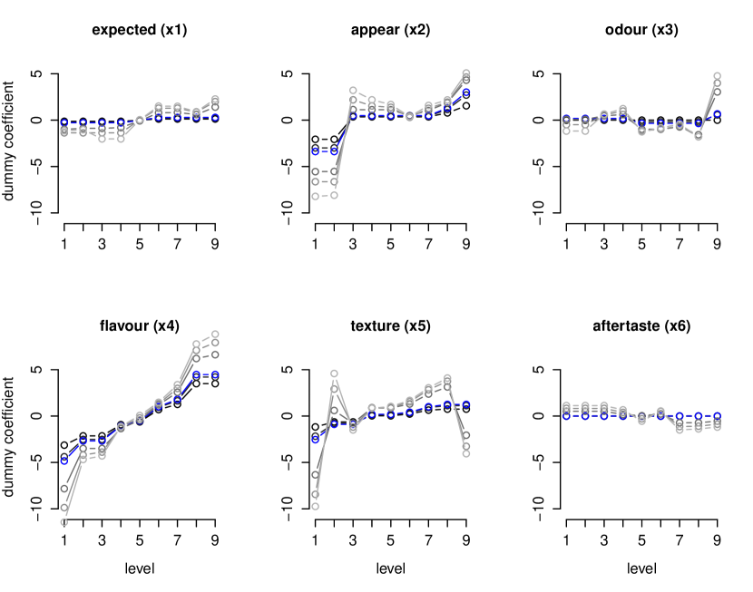
Figure 4: Cumulative fused lasso estimates of effect coded coefficients as functions of class labels ($\lambda\in\{10,5,1,0.5,0.25\}/n$).

Figure Figure 4 shows the fitted coefficients for covariates from Figure 3 when the fusion penalty (7) is employed. It is seen that some of the categories are fused, indicating that at least for some variables, fewer rating categories would be sufficient to model the effect on overall liking.

3.3 Tuning paramter, model and feature selection

3.3.1 Cross Validation

In the analysis discussed above, the penalty parameter $\lambda$ was fixed at some specific value. The choice of an optimal value for $\lambda$, however, should be made using the data at hand. Common strategies in penalized regression involve information criteria or cross-validation techniques. For $K$-fold cross-validation, the general procedure is that the data is randomly split into $K$ folds/subsets $k=1,\ldots,K$ of similar size. Given the $k$th subset is used as the so-called validation set, unknown parameters are fitted on the remaining $K-1$ parts of the data (the so-called training set). The model’s performance is then evaluated using an appropriate measure based on the predictions made on the $k$th subset of the data. As a measure of performance, we calculate the Brier Score (Brier, 1950) $\text{BS}=\sum_{i}\sum_{r}(y_{ir}-\pi_{ir})^{2}$, with the $c$-dimensional vector $\boldsymbol{y}_{i}=(y_{i1},\ldots,y_{ic})^{\top}$ of indicator variables, where $y_{ir}=1$ if $Y_{i}=r$, and zero otherwise.

Now, over a fine grid $G$ of sensible values $\lambda\in G$, the optimal $\lambda$ can be determined by minimizing the cross-validated Brier Score. The predictive performance on the boar-taint data for both the smooth group and fused lasso penalty as a function of $\lambda$ is given in Figure 5. On the training data, this function is monotonically increasing in $\lambda$, as with smaller $\lambda$ more emphasis is put on the data. On the validation data, however, we see that the unpenalized proportional odds model (see $\lambda\to 0$, i.e., $\log_{10}(\lambda)\to-\infty$) is clearly worse than smoothed selection or fusion. Cross-validation results indicate that predictive performance can indeed be enhanced when using the suggested penalized method(s). Performance improves on the validation data up to a certain $\lambda$ value and deteriorates from there. The optimal smoothing parameter, as determined on the validation set(s), is indicated by the dashed line in Figure 5 (right). Based on those results, we can use the optimal $\lambda$ (where the Brier Score on the validation data reaches its minimum) to refit the model.

Figure 5: Top: Brier Score with ordinal (smooth) selection penalty (averaged over all folds). Bottom: Brier Score with ordinal fusion penalty.

3.3.2 Stability Selection

The previous section described a potential process for selecting the regularization parameter. The choice of the regularization parameter, however, also implies the specific choice and number of features being selected. Particularly for high dimensional data, cross-validation techniques can be quite challenging as cross-validated choices may include too many variables (Meinshausen and Bühlmann, 2006; Leng et al., 2006). If we are mainly interested in feature selection, we can alternatively apply stability selection as suggested by Meinshausen and Bühlmann (2010), a promising subsampling strategy in combination with high dimensional variable selection. In general, instead of selecting/fitting one model, the data are perturbed or subsampled many times and we choose those variables that occur in a large fraction of runs. For every variable $\boldsymbol{x}_{j}$ the estimated probability $\hat{\pi}^{\lambda}_{j}$ of being in the stable selection set corresponds to the frequency of being chosen over all subsamples. Or, in other words, we keep variables with a high selection probability $\hat{\pi}^{\lambda}_{j}\geq\pi_{\text{thr}}$ and neglect those with low selection probability. The cutoff value can therefore be seen as a tuning parameter and a typical choice is $\pi_{\text{thr}}\in(0.6,0.9)$. Motivated by the concept of regularization paths, we then draw the stability path: the probability for each variable to be selected when randomly subsampling from the data as a function of $\lambda$. Meinshausen and Bühlmann (2010) emphasis that choosing the right regularization parameter is much less critical for the stability path which increases the chance of selecting truly relevant variables.

Figure 6 (top left) illustrates the coefficient path as a function of $\lambda$ for the sensory data from Section 2.1.1 and the smooth ordinal selection penalty (5). The objective of the study was to identify important factors for consumer acceptance of boar-tainted meat. Now, for the development of palatable products, it would be of great interest to detect the most important predictors for overall liking. Figure 6 (top right) also shows the stability path for selection penalty (5), indicating the order of relevance of the predictors according to stability selection. Analogously, Figure 6 (bottom) depicts the corresponding paths for fusion penalty (7). The probability to be selected within resampling is highest for flavour, texture, and appearance (in decreasing order). It can be concluded that the stability path is potentially useful for improved variable selection and interpretation.

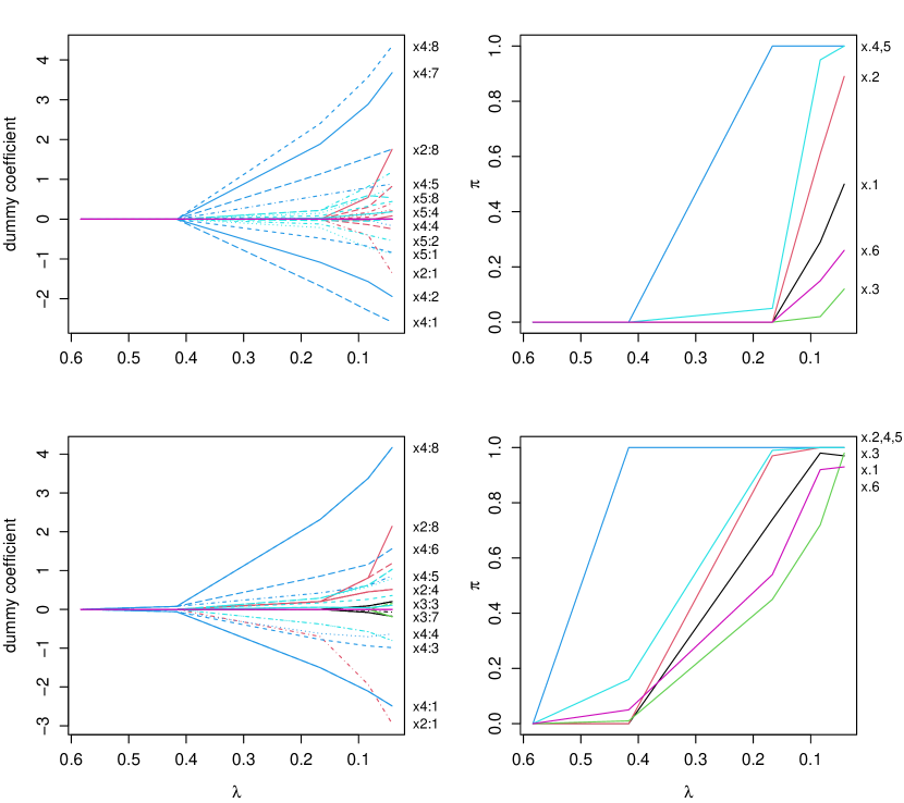
Figure 6: Top: Paths of cumulative smoothed lasso estimates of coefficients as functions of penalty parameter $\lambda\in\{70,50,20,10,5\}/n$ (left); Stability path of the cumulative smooth/ordinal lasso (right). Bottom: Corresponding paths of the cumulative fused lasso estimates.

4 Numerical Experiments

4.1 Study Design

Before applying the presented methodology to the luxury-food data in Section 5, we carry out a simulation study to investigate the properties of the proposed ordinal-on-ordinal selection approach using penalty (5) and (7), respectively. We compare both penalties to the usual approaches: (1) the standard cumulative logit model (polr) where the ordinal covariate is treated as nominal, i.e., it is dummy-coded without any penalization, and (2) treating the predictor as numeric (ordinalNet), i.e., the standard lasso penalty for selection. We generate $p=50$ ordinally scaled variables, including $38$ noise variables as follows: $\boldsymbol{x}_{1},\ldots,\boldsymbol{x}_{4}$ have non-monotone effects, $\boldsymbol{x}_{5},\ldots,\boldsymbol{x}_{8}$ are monotone but non-linear and the effect of $\boldsymbol{x}_{9},\ldots,\boldsymbol{x}_{12}$ is linear across categories. The remaining $38$ predictors are irrelevant, i.e., with zero effects. Each predictor is assumed to have the same number of levels, either five or nine, depending on the concrete setting considered. Factor levels are then randomly drawn from $\{1,...,5\}$ or $\{1,...,9\}$, respectively. The (true) covariate effects are shown in Figure 7. Using those predictors, we construct the ordinal response (with five levels) through the cumulative logit model (1) with linear predictor (3) and thresholds ${\boldsymbol{\theta}}=5.5,6.5,7.5,8.5$, and consider three different sample sizes ($n=200,500,1000$).

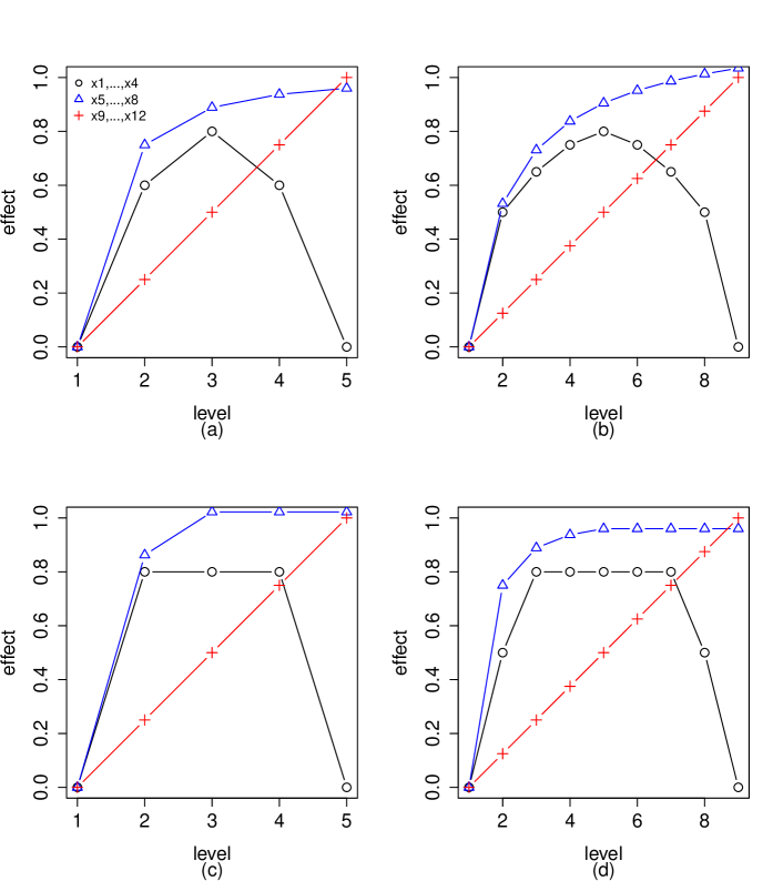
Figure 7: True effects of influential predictors. (a) $5$ levels without fused effects; (b) $9$ levels without fused effects; (c) $5$ levels with fused effects; (d) $9$ levels with fused effects.

We assign ranks to the predictor items according to the order of non-zero ordinal group lasso coefficients in the coefficient path and call this ordinal rank selection (ORS). For comparison, we fit a proportional odds model (POM) using polr with forward stepwise selection. In a similar manner, we proceed with the non-zero ordinal fused lasso coefficients in the corresponding coefficient path and call this ordinal rank fusion (ORF). Additionally, we fit a POM with the original lasso penalty using ordinalNet, treating predictors as numeric for selection purposes. The motivation behind this is that the usual ordinalNet function offers no (nominal/ordinal) group lasso option and thus selection for ordinal responses is only accessible if we ignore the categorical nature of the covariates. The entire process of data generation and estimation/selection was repeated 100 times. The results are discussed below.

4.2 Results

4.2.1 Variable Selection

To evaluate the methods’ performance in terms of variable selection, we construct the Receiver Operating Characteristic (ROC) by varying selection thresholds $\lambda$ (for ORS, ORF, and ordinalNet) and calculate the Area Under this Curve (AUC, true positive rate vs. false positive rate) in each iteration. Briefly, we evaluate the estimated models as a binary classification task, where covariates are predicted to be present or absent. For polr, the order of variables entering the (forward) stepwise selected model is used for ranking. Variables that were not selected at all are randomly coerced to the back. We only discuss the results of scenario (a) from Figure 7 in detail here, where true effects contain unfused effects of $5$ levels. Due to a lack of space, we refer to the supplementary material in Appendix C for the results of the other settings considered.

Figure 8: ROC curves when using ORS, polr, ORF, or ordinalNet with $n=200$. According to setting (a) from Figure 7 ($5$ levels without fused effects).

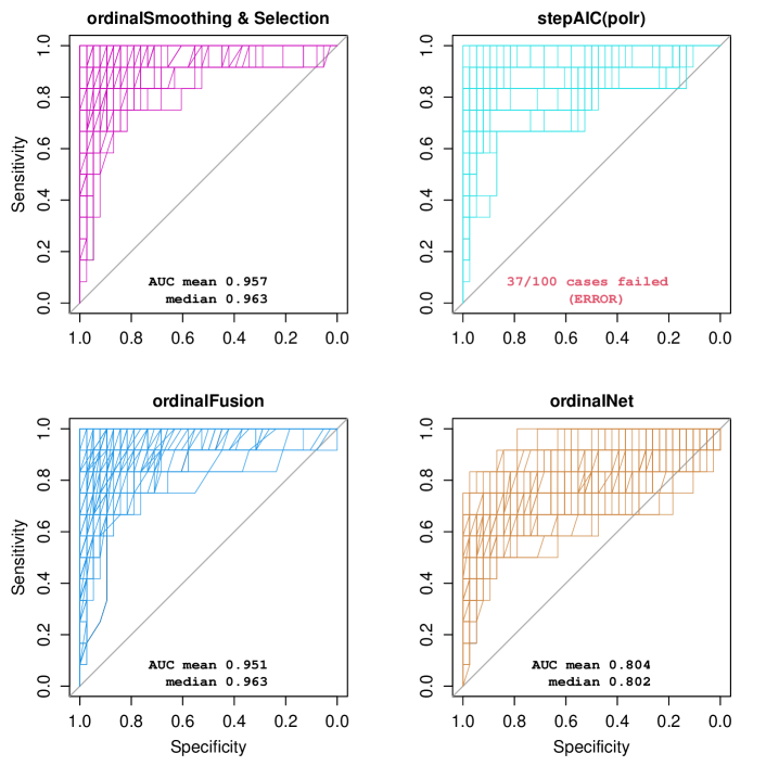
Figure 9: ROC curves when using ORS, polr, ORF, or ordinalNet with $n=500$. According to setting (a) from Figure 7 ($5$ levels without fused effects).

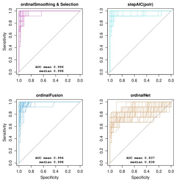
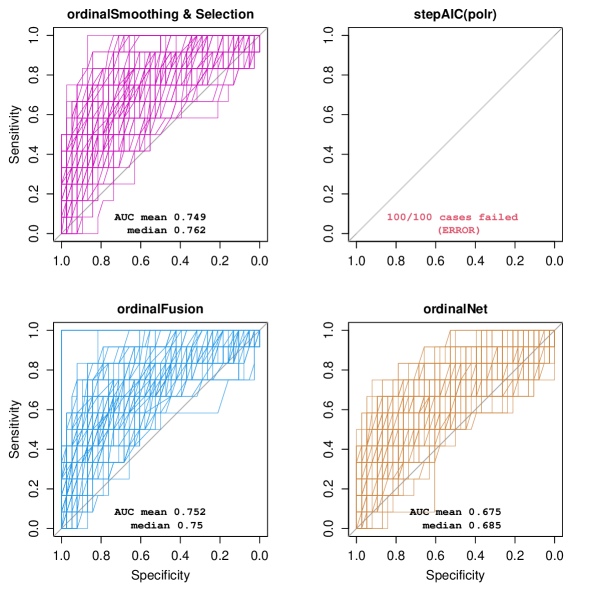
Figure S10: ROC curves when using ORS, polr, ORF or ordinalNet with n = 1000. According to setting (a) from Figure S1 ($\mathbf{5}$ levels without fused effects).

Figure S11: ROC curves when using ORS, polr, ORF or ordinalNet with n = 200. According to setting (b) from Figure S1 ($\mathbf{9}$ levels without fused effects).

Figures 8 and 9 show the performance in terms of the ROC as obtained with varying $\lambda$ values, $n=200$ and $n=500$, respectively. Additionally, the mean and median AUC for each method is given. The results for the remaining scenarios can be found in Appendix C (Figures S8–S19). Even given the relatively large sample size of $500$, polr failed in $37$ of the datasets (zero cases with $n=1000$, but all cases with $n=200$). This result is in line with the issues that we observed with the standard POM for the boar-taint data in the previous section. The mean and median AUC over the 63 successful runs with $n=500$ were $0.908$ and $0.919$, respectively. By contrast, we see that the ordinal penalties work very well and both account for the ordinal-on-ordinal nature. In general, the choice between penalties (5) and (7) depends on the concrete application and/or personal preferences. While both enforce the selection of predictors, ORS yields smooth effects of predictors, whereas ORF yields parameter estimates that tend to be flat over some neighbouring categories, which represents a specific form of smoothness, too. The classical ordinalNet approach, however, is inferior for model selection since it offers no group lasso option for categorical/ordinal predictors. With $n=1000$ (not shown here) all methods –except of classical lasso– work (almost) equally well concerning scenarios (a) and (c). With scenarios (b) and (d), i.e., with predictors having nine levels each, polr performs even worse than Figure 9 (top right), as estimation now fails in all cases with $n=500$. Even with $n=1000$, polr is inferior to penalized selection and fusion in the nine predictor level setting (compare Appendix C for details, Figures S11–13 and S17–19).

4.2.2 Level Fusion

Results discussed so far concerned the identification of relevant predictors. In scenarios (c) and (d), however, we are also interested in comparing the performance regarding the identification of relevant differences (i.e., fusion/clustering) between adjacent dummy coefficients. For this purpose, we consider estimates using penalty (7).

Figure 10: ROC curves when using polr or ordinalNet concerning the identification of relevant differences (i.e., fusion) of dummy coefficients for $n=1000$. Top: $5$ levels with fused effects; bottom: $9$ levels with fused effects.

Figure 10 (right) shows the performance in terms of ROC as obtained with varying $\lambda$ and $n=1000$. In addition, we run stepAIC(polr) (Figure 10, left) as a competing model, but on the split-coded design matrix, thus selecting (presumably relevant) differences between neighbouring categories. The run time of polr increases dramatically, as factor levels now enter and leave the model in each step separately. Figure S21 in Appendix C illustrates the false positive/negative rates (FPR/FNR). With five underlying levels (scenario (c)) and $n=500$, stepAIC(polr) only converged in 23 cases, and, not surprisingly, in zero cases for $n=200$. This is why we only present results for the largest sample size $n=1000$. With nine underlying levels (scenario (d)), estimation with polr failed in all cases with $n=200$ and $n=500$. The poorer performance compared to variable selection (see Figures S16 and S19, Appendix C) can be explained by the fact that with selection it is sufficient for a correct result (in terms of a ‘true positive’) if at least one contrast was selected. For identification of the relevant differences, however, all contrasts of neigbouring categories are checked individually. With nine predictor levels (Figure 10, bottom), the model has even more parameters that have to be taken into account, which further worsens the results. Overall, we can conclude that estimation with the fusion penalty also performs better than stepwise selection with respect to the identification of relevant differences between neigbouring categories.

5 Consumers’ Willingness to Pay for Luxury Food

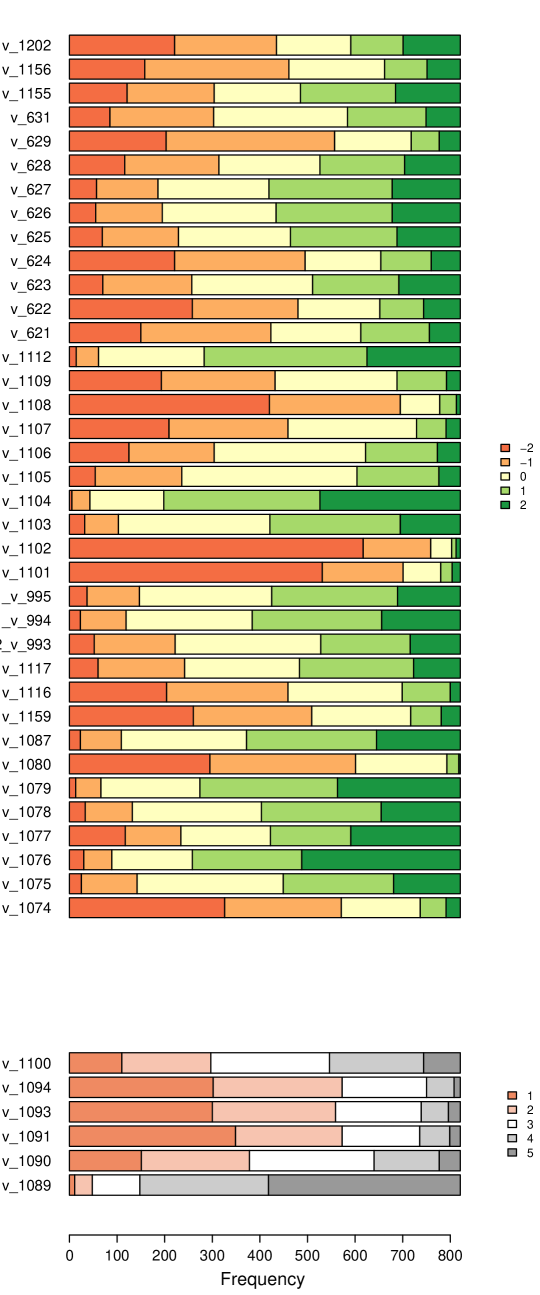
Figure S1: Summary for items of the luxury food dataset on individual level. Coding scheme for items: $-2$ ‘strong rejection’ to 2 ‘strong agreement’ (top) or 1 ‘never’ to 5 ‘very often’ (bottom).

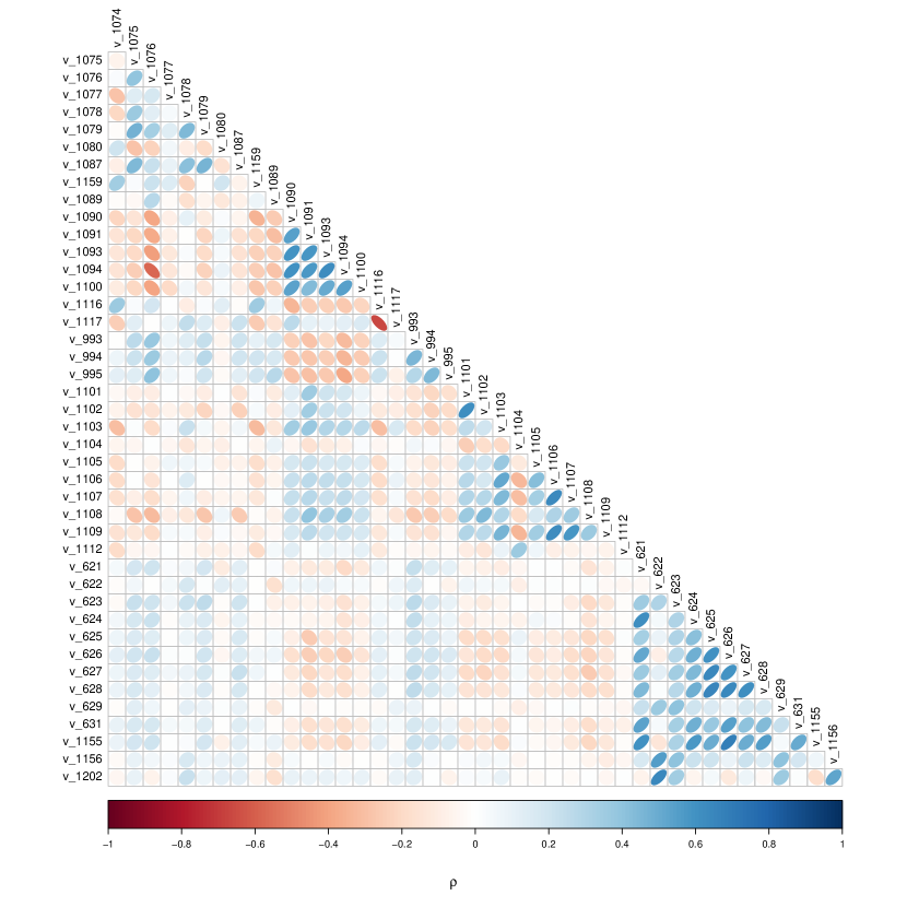
Figure S7: Correlation plot of the luxury data set.

We use penalties (5) and (7) when modelling the luxury food data described in the Introduction. The descriptive statistics on the data analyzed can be found in the supplementary material (Appendix C), covering, inter alia, a description of the items along with observed frequencies (Table S1 and Figure S1) and the correlation plot (Figure S7). For more details on the dataset, we refer to Hartmann et al. (2016) who performed a partial least squares structural equation analysis (treating, however, the data as numeric). Using an initial principal component analysis (also treating the data as numeric), the authors reveal seven relevant dimensions with respect to the consumers’ attitudes towards luxury food, namely, hedonism, quality, sustainability, materialism, usability, uniqueness, and price. In our analysis, by contrast, the research question is more specific, in the sense that we try to identify factors that determine the consumers’ willingness to pay for food products that they associate with luxury.

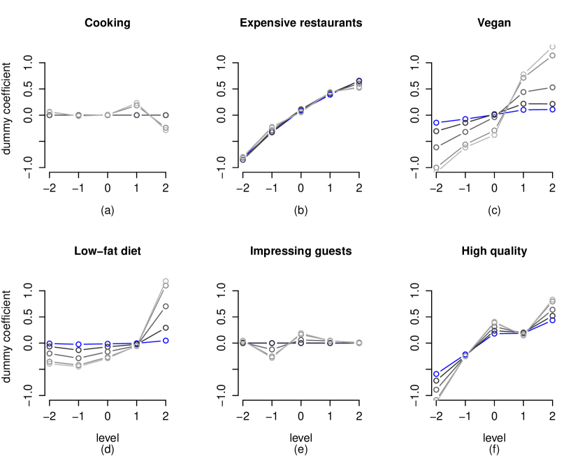
Figure 11: Cumulative group lasso estimates of effect coded coefficients as functions of class labels ($\lambda\in{14.5,10,5,1,0.25}/n$). Light gray indicates smaller $\lambda$.

Figure 11 illustrates the resulting estimates of selected covariates and different values of tuning parameter $\lambda$ when applying the ordinal group lasso. Figure 12 shows the corresponding results for the ordinal fused lasso. For smaller $\lambda$ (light gray), the estimates are more wiggly and become more and more smoothed out/shrunk as $\lambda$ increases. Especially, the willingness to pay tends to increase among people who (a) eat out frequently in expensive restaurants, (c) associate a high price with good quality, and (f) associate luxury with high quality.

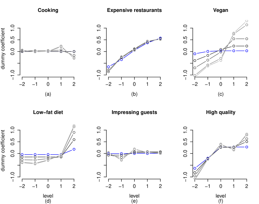
Figure 12: Cumulative fused lasso estimates of effect coded coefficients as functions of class labels ($\lambda\in{18.5,10,5,1,0.25}/n$). Light gray indicates smaller $\lambda$.

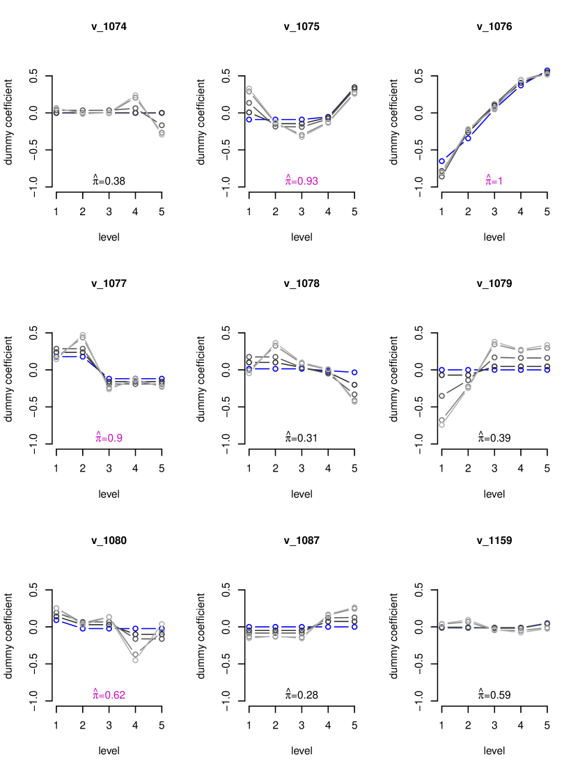
Figure S2: Cumulative fused lasso estimates of effect coded coefficients as functions of class labels ($\lambda\in\{18.5,10,5,1,0.25\}/n$) along with selection frequencies $\hat{\pi}$. Selected variables according to thresholds $\pi_{thr}=0.6$ are highlighted in magenta (where $\lambda$ was set to $15/n$ to achieve comparable results with group lasso). Blue lines correspond to cross-validated/optimal $\lambda=18.5/n$.

Our findings thus contribute to the literature on food and/or luxury by indicating which kind of consumers may be particularly willing to pay a higher price for ‘luxury food’. From a more general perspective, Wiedmann et al. (2009) and Shirai (2015) already discussed the perceived association of luxury, quality, and price. Alfnes and Sharma (2010) and Parsa et al. (2017) specifically consider customers in restaurants, highlight price as a perceived positive indicator for the quality of food, and investigate ways to increase the willingness to pay, respectively. An overview of the estimated effects of all items considered in our study is given in Appendix C (Figures S2–S6). Since the effects of penalties (5) and (7) are quite similar, only the results of the fused lasso are presented there. For some items, e.g., “I like to cook myself” (v_1074) and “Luxury food can impress my guests” (v_623), we observe rather flat effects that quickly go to zero as soon as $\lambda$ is increases, indicating that those items provide only limited information regarding the respondent’s willingness to pay for luxury food. In other words, for a producer of luxury food, it might not be worth targeting consumers that primarily want to ‘show off’ (compare v_623).

The (5-fold) cross-validated predictive performance in terms of the Brier score  (Brier, 1950) as a function of $\lambda$ is given in Figure 13 (top: group lasso; bottom: fused lasso).

Figure 13: Top: Brier Score with ordinal (smooth) selection penalty (averaged over all folds). Bottom: Brier Score with ordinal fusion penalty.

If using the fused lasso and choosing the amount of penalty through (5-fold) cross-validation, we obtain an optimal $\lambda$ around $18.5/n$ (marked by the dashed line in Figure 13, bottom right). The corresponding estimates of the covariates’ effects are highlighted in blue in Figure 12. For the variable (f) “Luxury food has a good quality”, for example, it is seen that the upper three categories are fused. If using the ordinal group lasso instead, the optimal (cross-validated) $\lambda$ is around $14.5/n$ (marked by the dashed line in Figure 13, top right), with the resulting estimates in Figure 11 indicated by the blue lines. If choosing $\lambda=14.5/n$ to obtain a final model, 17 variables are removed and 26 variables are selected by the ordinal group lasso, with some showing very small effects though. The most influential factors are those already shown in Figure 11: (a) Expensive restaurants, (c) associating a high price with good quality, and (f) associating luxury with high quality. With the fused lasso, however, we might be more interested in detecting significant differences. To obtain an idea of the complexity of the fitted model, we refer to the degrees of freedom (df). For the fused lasso, an approximation is given by the number of non-zero parameters, i.e., non-zero differences of adjacent (dummy) coefficients (cf. Tibshirani et al., 2005). If using $\lambda=18.5/n$ for the ordinal fused lasso, we detect 51 relevant differences, which corresponds to about one-third compared to a total of $43\times 4=172$ parameters in the full model.

6 Discussion

In the present work, we proposed a method for variable selection in item-on-items regression. Based on tailored regularization tools, the approach effectively extracts information from ordinally scaled predictors and accounts for ordinal response variables. In particular, an $L_{2}$-difference penalty of first order for the selection of relevant factors and an $L_{1}$ variant for fusion of categories were presented. Our approach is more flexible than those existing for ordinal responses in combination with ordinal predictors so far and allows for smoothing of covariate effects. The proposed method is implemented in R and publicly available on Github and soon on CRAN through add-on package ordPens.

To illustrate the application and potential benefits of item-on-items selection in practice, we presented two motivating data examples. First, we considered a survey on consumers’ acceptance of the use of boar-tainted meat consisting of seven Likert-type items with nine levels each. In summary, our presented results suggest that penalized item-on-items regression works well in the cumulative logit model with ordinally scaled predictors and ordinal group or fused lasso penalty. We combined the penalty approach with stability selection to gain additional information about a variable’s probability to be selected, given a defined $\lambda$ value. Namely, the stability path revealed that the probability to be selected (within resampling) is highest for flavour, texture, and appearance.

For comparison, we considered the standard proportional odds model implemented in the polr() R-function, which simply treats categorical/ordinal covariates as dummy-coded factors and offers no option for smoothing. We found that the use of polr can cause problems as (a) the employed fitting routine often fails (even for moderately dimensioned setups) and (b) often results in wiggly/implausible estimates of the (categorical) covariates’ effects. In our numerical experiments, we distinguished between settings involving five or nine predictor levels. In summary, polr only worked well when the sample size was large enough and (often) failed otherwise. Ordinal selection and ordinal fusion worked equally well and outperformed polr by far in most scenarios. Overall performance deteriorated with an increasing number of category levels. In addition, we compared our smoothing/selection and fusion penalties to the classical lasso for the cumulative logit model as implemented in ordinalNet(). This method offers no group lasso option for the selection of categorical predictors. In our numerical experiments, it was thus not particularly surprising that in terms of AUC values, standard ordinalNet with linear effects performed worst and therefore seems somewhat unsuited for item-on-items regression if at least some of the effects may be non-linear across factor levels or even non-monotone.

Our main interest was in a high-dimensional survey on luxury food expenditure, again consisting of Likert-type items. On the one hand, in a data set of this size, not all of the items will be relevant for explaining the response, making variable selection a primary concern. On the other hand, we would like to have estimates that are rather smooth and interpretable, while incorporating the covariates’ ordinal scale level. As a consequence, penalized (cumulative logit) regression appears to be a sensible approach in studies of this type. For some items, we could observe that most categories are fused. For some (presumably) less relevant items, we could see that they reach effects equal to zero as $\lambda$ increases. To obtain a final model, the optimal $\lambda$ was chosen using cross-validation. With the group lasso, about 40% of the covariates were removed from the model. With the fused lasso, we detected about one-third of the parameters (in the sense of non-zero differences between adjacent categories) to be relevant.

Appendix A Maximum Likelihood Estimation in the Cumulative Logit Model

To embed the cumulative logit model into the framework of generalized linear models (GLMs), we first introduce the response function as well as the design matrix. The occurrence probability $P(Y_{i}=r)=P(y_{ir}=1)=\pi_{ir}$ in model (1) is connected to the linear predictor $\eta_{ir}$ via the response function $h_{r}(\boldsymbol{\eta}_{i})$ as follows:
$\pi_{i1}=h_{1}(\eta_{i1},\ldots,\eta_{ic})=F(\eta_{i1})$ and

$$\pi_{ir}=h_{r}(\eta_{i1},\ldots,\eta_{ic})=F(\eta_{ir})-F(\eta_{i,r-1}),\quad r=2,\ldots,c$$

with

$$\eta_{ir}=\theta_{r}+x_{i1}\beta_{1}+\ldots+x_{ip}\beta_{p}$$

and $F(\eta_{ir})=1/(1+\exp(-\eta_{ir}))$ being the logistic distribution function.

In matrix notation, we can write $\boldsymbol{\eta}_{i}=\boldsymbol{X}_{i}\boldsymbol{\gamma}$ with

$$\boldsymbol{X}_{i}=\begin{pmatrix}1&&&&\boldsymbol{x}^{\top}_{i}\\ &1&&&\boldsymbol{x}^{\top}_{i}\\ &&\ddots&&\vdots\\ &&&1&\boldsymbol{x}^{\top}_{i}\\ \end{pmatrix}$$

and the parameter vector $\boldsymbol{\gamma}=(\theta_{1},\ldots,\theta_{c-1},\boldsymbol{\beta})^{\top}$.

The $c$-dimensional response function is given by $\boldsymbol{\pi}_{i}=\boldsymbol{h}(\boldsymbol{\eta}_{i})$. Again let $(y_{i1},\ldots,y_{ic})$ be binary indicators of the response for subject $i$. Then, the log-likelihood for the sample has the form

$$l(\boldsymbol{\gamma})=\sum_{i=1}^{n}\sum_{r=1}^{c}y_{ir}\log{\pi_{ir}}=\sum_{i=1}^{n}\boldsymbol{y}_{i}\log\big{\{}\boldsymbol{h}(\boldsymbol{\eta}_{i})\big{\}}.$$

with

$$h_{r}(\eta_{ir})=\left\{\begin{array}[]{ll}\frac{\exp{(\eta_{ir})}}{1+\exp{(\eta_{ir})}},&r=1\\ \frac{\exp{(\eta_{ir})}}{1+\exp{(\eta_{ir})}}-\frac{\exp{(\eta_{i,r-1})}}{1+\exp{(\eta_{i,r-1})}},&r=2,\cdots,c\end{array}\right..$$

Based on the exponential family, the score function $\boldsymbol{s}(\boldsymbol{\gamma})=\partial l(\boldsymbol{\gamma})/\partial\boldsymbol{\gamma}$ takes the form

$$\boldsymbol{s}(\boldsymbol{\gamma})=\sum_{i=1}^{n}\boldsymbol{X}_{i}^{\top}\boldsymbol{D}_{i}(\boldsymbol{\gamma})\boldsymbol{\Sigma}_{i}^{-1}(\boldsymbol{\gamma})[\boldsymbol{y}_{i}-\boldsymbol{h}(\boldsymbol{\eta}_{i})],$$

where $\boldsymbol{D}_{i}(\boldsymbol{\gamma})=\partial\boldsymbol{h}(\boldsymbol{\eta}_{i})/\partial\boldsymbol{\eta}$ denotes the derivative of $\boldsymbol{h}(\boldsymbol{\eta})$ evaluated at $\boldsymbol{\eta}_{i}=\boldsymbol{X}_{i}\boldsymbol{\gamma}$ and $\boldsymbol{\Sigma}_{i}(\boldsymbol{\gamma})=\text{cov}(\boldsymbol{y}_{i})$ is the covariance matrix of observation vector $\boldsymbol{y}_{i}=(y_{i1},\ldots,y_{ic})$ given parameter vector $\boldsymbol{\gamma}$. By introducing the weight matrix $\boldsymbol{W}_{i}(\boldsymbol{\gamma})=\boldsymbol{D}_{i}(\boldsymbol{\gamma})\boldsymbol{\Sigma}_{i}^{-1}(\boldsymbol{\gamma})\boldsymbol{D}_{i}^{\top}(\boldsymbol{\gamma})$, we can write the expected Fisher matrix as

$$\boldsymbol{F}(\boldsymbol{\gamma})=\text{cov}(\boldsymbol{s}(\boldsymbol{\gamma}))=\sum_{i=1}^{n}\boldsymbol{X}_{i}^{\top}\boldsymbol{W}_{i}(\boldsymbol{\gamma})\boldsymbol{X}_{i}=\text{E}(-\nabla^{2}l(\boldsymbol{\gamma})).$$

Note that in order to incorporate categorical/ordinal predictors, we have to replace $p$-dimensional vectors $\boldsymbol{x}_{i}^{\top}$ by corresponding dummy vectors $\boldsymbol{z}_{i}=(\boldsymbol{z}_{i1}^{\top},\ldots,\boldsymbol{z}_{ip}^{\top})^{\top}$. Then, $\boldsymbol{\gamma}$ collects all regression parameters (thresholds plus regression coefficients) to be estimated, potentially after reparametrization to respect constraints as described in Section 2.2.

Appendix B Algorithm of Penalized Item-on-Items Regression

In this appendix, the algorithm behind the method explained previously, is briefly outlined. The main idea is to combine a quadratic approximation of the log-likelihood $l(\cdot)$ with an additional line search. In particular, we utilize and modify the block coordinate gradient descent method of Tseng and Yun (2009).

Using a second-order Taylor series expansion at $\hat{\boldsymbol{\beta}}^{(t)}$, i.e., at the current estimate in iteration $t$ of the algorithm, and replacing the Hessian of $l(\cdot)$ by some suitable matrix $\boldsymbol{H}^{(t)}$ we specify

$$\begin{split}M_{\lambda}^{[t]}(\textbf{\text{d}})&=-\Bigl{\{}l(\boldsymbol{\gamma}^{[t]})+\textbf{\text{d}}^{\top}\nabla l(\boldsymbol{\gamma}^{[t]})+\frac{1}{2}\textbf{\text{d}}^{\top}\boldsymbol{H}^{(t)}\textbf{\text{d}}\Bigr{\}}+\lambda\sum_{j=1}^{p}\sqrt{k_{j}}||\boldsymbol{D}_{1,j}\boldsymbol{\beta}_{j}^{[t]}+\textbf{\text{d}}_{j}||_{2}\\ &\approx l_{\lambda}(\boldsymbol{\gamma}^{[t]}+\textbf{\text{d}}),\end{split}$$ (8)

where $\textbf{\text{d}}\in\mathbb{R}^{p+(c-1)}$ and $\boldsymbol{D}_{1,j}$ is defined in equation (6). Minimization of $M_{\lambda}^{[t]}(\textbf{\text{d}})$ is carried out with respect to the $j$th parameter group. Then, we assume the ($k_{j}\times k_{j}$) submatrix $\boldsymbol{H}^{(t)}=h_{j}^{(t)}\boldsymbol{I}_{k_{j}}$ for some scalar $h_{j}^{(t)}\in\mathbb{R}$, where a possible choice is

$$h_{j}^{(t)}=\min\{\max\{\text{diag}(\nabla^{2}l(\hat{\boldsymbol{\gamma}}^{(t)})_{jj}),10^{-6}\},10^{8}\}$$

and $\boldsymbol{I}_{k_{j}}$ is the identity matrix of corresponding dimensions.

If

$$||\nabla l(\hat{\boldsymbol{\gamma}}^{(t)})_{j}-h_{j}^{(t)}\hat{\boldsymbol{\beta}}^{(t)}_{j}||_{2}\leq\lambda\sqrt{k_{j}},$$ (9)

the minimizer of $M_{\lambda}^{[t]}(\textbf{\text{d}})$ in (8) w.r.t. to group $j$ is

$$\textbf{\text{d}}^{(t)}_{j}=-\hat{\boldsymbol{\beta}}_{j}^{(t)}.$$

Otherwise

$$\textbf{\text{d}}^{(t)}_{j}=-\frac{1}{h_{j}^{(t)}}\Bigg{\{}\nabla l(\hat{\boldsymbol{\gamma}}^{(t)})_{j}-\lambda\sqrt{k_{j}}\frac{\nabla l(\hat{\boldsymbol{\gamma}}^{(t)})_{j}-h_{j}^{(t)}\hat{\boldsymbol{\beta}}_{j}^{(t)}}{||\nabla l(\hat{\boldsymbol{\gamma}}^{(t)})_{j}-h_{j}^{(t)}\hat{\boldsymbol{\beta}}_{j}^{(t)}||_{2}}\Bigg{\}}.$$

If $\textbf{\text{d}}^{(t)}\neq 0$, an (inexact) line search using the Armijo rule must be performed. Let $\alpha^{(t)}$ be the largest value among the grid $\{\alpha_{o}\delta^{l}\}_{l\geq 0}$ s.t.

$$l_{\lambda}(\hat{\boldsymbol{\gamma}}^{(t)}+\alpha^{(t)}\textbf{\text{d}}^{(t)})-l_{\lambda}(\hat{\boldsymbol{\gamma}}^{(t)})\leq\alpha^{(t)}\sigma\Delta^{(t)},$$

where $0<\sigma<1$, $\alpha_{0}>0$ and $\Delta^{(t)}$ is the improvement in $l_{\lambda}(\cdot)$ when using a linear approximation for the objective function

$$\Delta^{(t)}=-\textbf{\text{d}}^{(t)\top}\nabla l(\hat{\boldsymbol{\gamma}}^{(t)})_{j}+\lambda\sqrt{k_{j}}||\hat{\boldsymbol{\beta}}_{j}^{(t)}+\textbf{\text{d}}_{j}^{(t)}||_{2}-\lambda\sqrt{k_{j}}||\boldsymbol{D}_{1,j}\hat{\boldsymbol{\beta}}_{j}^{(t)}||_{2}.$$

Standard choices are $\alpha_{0}=1$, $\delta=0.5$ and $\sigma=0.1$. Finally, we specify

$$\hat{\boldsymbol{\beta}}^{(t+1)}=\hat{\boldsymbol{\beta}}^{(t)}+\alpha^{(t)}\textbf{\text{d}}^{(t)}.$$

The described procedure, namely

• looping through the block coordinates $\{1,\ldots,p\}$:

• update $\boldsymbol{H}_{j}^{(t)}\leftarrow h_{j}(\gamma^{(t)})\boldsymbol{I}_{k_{j}}$

• $\textbf{\text{d}}^{(t)}\leftarrow\text{arg min}\{M_{\lambda}^{(t)}(\textbf{\text{d}})\}$

• if $\textbf{\text{d}}^{(t)}\neq 0$
  $\alpha^{(t)}\leftarrow$ line search
  $\boldsymbol{\beta}^{(t+1)}\leftarrow\boldsymbol{\beta}^{(t)}+\alpha^{(t)}\textbf{\text{d}}^{(t)}$

is repeated until some convergence criterion is met.

Note that the check for differentiability in condition (9) is not necessary for the intercept parameters (because those parameters are not penalized) and the solution can be directly computed as

$$\textbf{\text{d}}_{\theta}^{\top}=-\frac{1}{h_{\theta}^{(t)}}\nabla l(\hat{\boldsymbol{\gamma}}^{(t)})_{\theta},$$

where the index denotes the elements belonging to $\theta_{1},\ldots,\theta_{c-1}$.

Appendix C Supplementary Results

	Eating habits
v_1074	I like to cook myself.
v_1075	I often go out to eat at inexpensive restaurants, snack bars or cafes.
v_1076	I often go out to eat at more expensive restaurants.
v_1077	Most of the time another family member cooks for me.
v_1078	I often buy ready-made products.
v_1079	I often order from a delivery service (e.g. pizza service).
v_1080	I prefer to eat at home.
v_1087	I often just take something from the bakery (or similar) instead of big meals.
v_1159	On weekends, we (my family and I/my friends and I) take a lot of time to eat together.
Coding:	$-2=$ ‘not true at all’, $\ldots\,$, $2=$ ‘absolutely true’
	Shopping places: Where do you buy most of your food?
v_1089	In discount stores (e.g. Aldi, Lidl, Netto, Penny).
v_1090	At the weekly market.
v_1091	In the organice food store (e.g. Alnatura).
v_1093	In the farm store.
v_1094	In the delicatessen store.
v_1100	In the specialized trade (e.g. meat, cheese, fruit/vegetable, wine store).
Coding:	$1=$ ‘never’, $\ldots\,$, $5=$ ‘very often’
	Shopping habits (purchasing involvement)
v_1116	I like to take my time shopping for groceries.
v_1117	Food shopping has to be fast for me.
Coding:	$-2=$ ‘strongly disagree’, $\ldots\,$, $2=$ ‘fully agree’
	What importance does the price of food have for you? (price-value)
dupl2_v_993	I associate a high price in food with particularly good quality.
dupl1_v_994	I am more likely to buy a certain food item if the price is comparatively high.
dupl1_v_995	When buying food, the price for me is completely undecisive.
Coding:	$-2=$ ‘strongly disagree’, $\ldots\,$, $2=$ ‘fully agree’
	Nutrition style
v_1101	Vegetarian.
v_1102	Vegan.
v_1103	I pay attention to a healthy diet.
v_1104	I eat everything I like.
v_1105	I eat in small quantities.
v_1106	I eat a low-fat diet.
v_1107	I eat a low-carbohydrate diet.
v_1108	I eat a functional diet (e.g. sports nutrition).
v_1109	I eat slimming.
v_1112	I eat a little bit of everything.
Coding:	$-2=$ ‘not true at all’, $\ldots\,$, $2=$ ‘absolutely true’
	Luxury food
v_621	…has a particularly fine taste.
v_622	…is particularly expensive.
v_623	…can impress my guests.
v_624	…has a particularly high quality.
v_625	…comes from organic farming.
v_626	…comes from regional cultivation.
v_627	…bears a fair trade seal.
v_628	…it comes from particularly species-appropriate animal husbandry.
v_629	…has a certain rarity value.
v_631	…is a specialty of a country/region.
v_1155	…is particularly fresh.
v_1156	…has an exclusive brand.
v_1202	…tends to be consumed by the rich/better off.
Coding:	$-2=$ ‘I do not associate with luxury at all’, $\ldots\,$, $2=$ ‘I strongly associate with luxury’

Table S1: Items of the luxury food dataset.

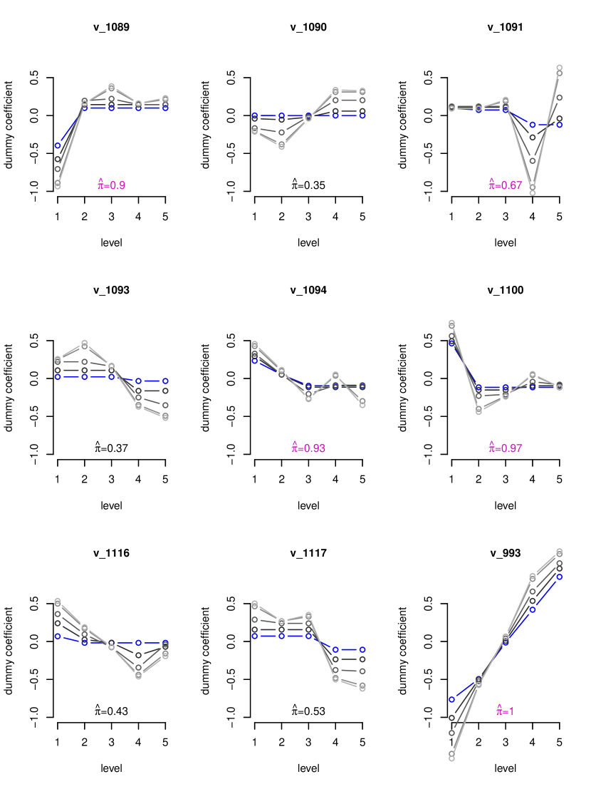
Figure S3: Cumulative fused lasso estimates of effect coded coefficients as functions of class labels ($\lambda\in\{18.5,10,5,1,0.25\}/n$) along with selection frequencies $\hat{\pi}$. Selected variables according to thresholds $\pi_{thr}=0.6$ are highlighted in magenta (where $\lambda$ was set to $15/n$ to achieve comparable results with group lasso). Blue lines correspond to cross-validated/optimal $\lambda=18.5/n$.

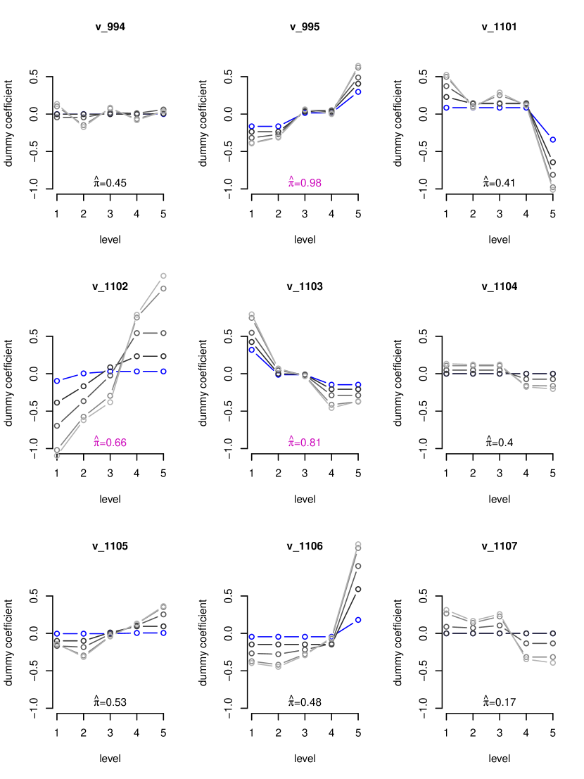
Figure S4: Cumulative fused lasso estimates of effect coded coefficients as functions of class labels ($\lambda\in\{18.5,10,5,1,0.25\}/n$) along with selection frequencies $\hat{\pi}$. Selected variables according to thresholds $\pi_{thr}=0.6$ are highlighted in magenta (where $\lambda$ was set to $15/n$ to achieve comparable results with group lasso). Blue lines correspond to cross-validated/optimal $\lambda=18.5/n$.

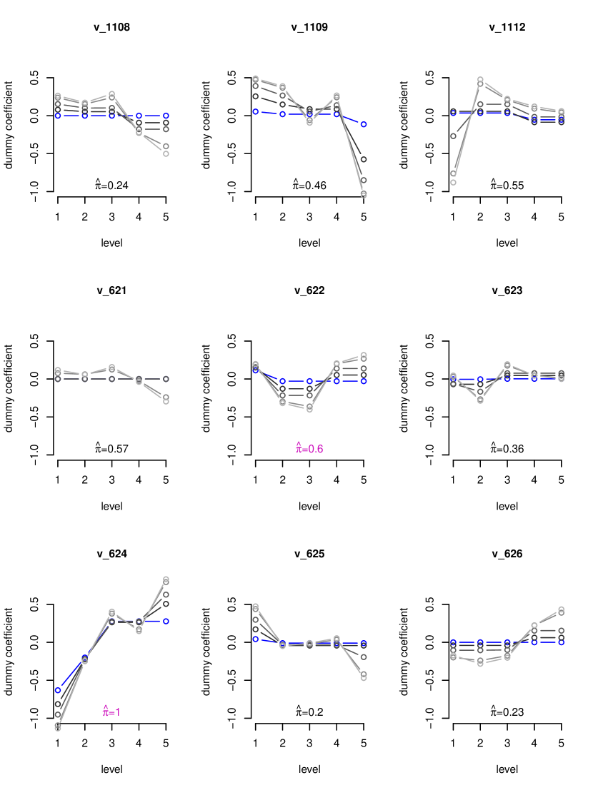
Figure S5: Cumulative fused lasso estimates of effect coded coefficients as functions of class labels ($\lambda\in\{18.5,10,5,1,0.25\}/n$) along with selection frequencies $\hat{\pi}$. Selected variables according to thresholds $\pi_{thr}=0.6$ are highlighted in magenta (where $\lambda$ was set to $15/n$ to achieve comparable results with group lasso). Blue lines correspond to cross-validated/optimal $\lambda=18.5/n$.

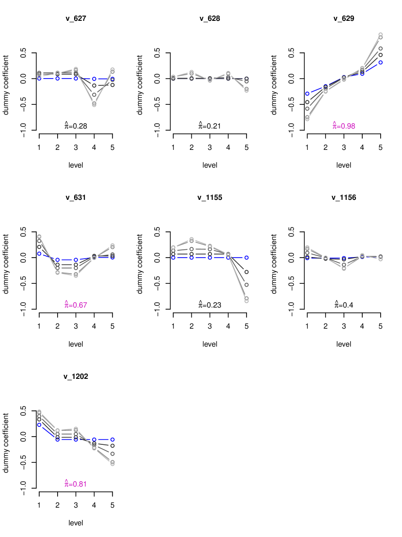
Figure S6: Cumulative fused lasso estimates of effect coded coefficients as functions of class labels ($\lambda\in\{18.5,10,5,1,0.25\}/n$) along with selection frequencies $\hat{\pi}$. Selected variables according to thresholds $\pi_{thr}=0.6$ are highlighted in magenta (where $\lambda$ was set to $15/n$ to achieve comparable results with group lasso). Blue lines correspond to cross-validated/optimal $\lambda=18.5/n$.

Figure S8: ROC curves when using ORS, polr, ORF or ordinalNet with n = 200. According to setting (a) from Figure S1 ($\mathbf{5}$ levels without fused effects).

Figure S9: ROC curves when using ORS, polr, ORF or ordinalNet with n = 500. According to setting (a) from Figure S1 ($\mathbf{5}$ levels without fused effects).

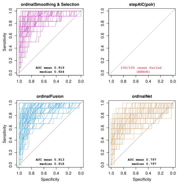
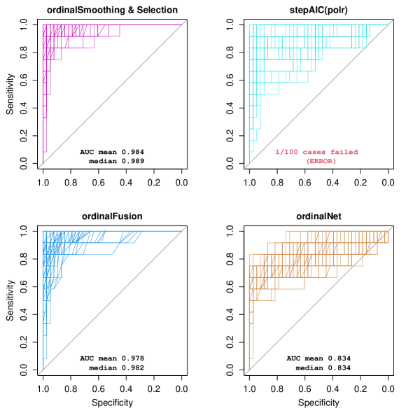
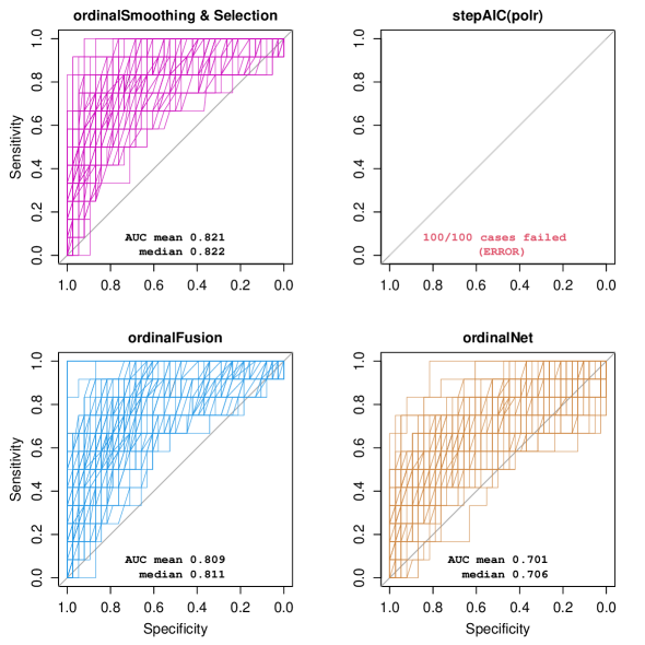
Figure S12: ROC curves when using ORS, polr, ORF or ordinalNet with n = 500. According to setting (b) from Figure S1 ($\mathbf{9}$ levels without fused effects).

Figure S13: ROC curves when using ORS, polr, ORF or ordinalNet with n = 1000. According to setting (b) from Figure S1 ($\mathbf{9}$ levels without fused effects).

Figure S14: ROC curves when using ORS, polr, ORF or ordinalNet with n = 200. According to setting (c) from Figure S1 ($\mathbf{5}$ levels with fused effects).

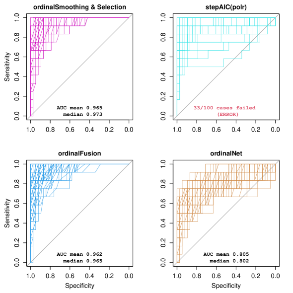
Figure S15: ROC curves when using ORS, polr, ORF or ordinalNet with n = 500. According to setting (c) from Figure S1 ($\mathbf{5}$ levels with fused effects).

Figure S16: ROC curves when using ORS, polr, ORF or ordinalNet with n = 1000. According to setting (c) from Figure S1 ($\mathbf{5}$ levels with fused effects).

Figure S17: ROC curves when using ORS, polr, ORF or ordinalNet with n = 200. According to setting (d) from Figure S1 ($\mathbf{9}$ levels with fused effects).

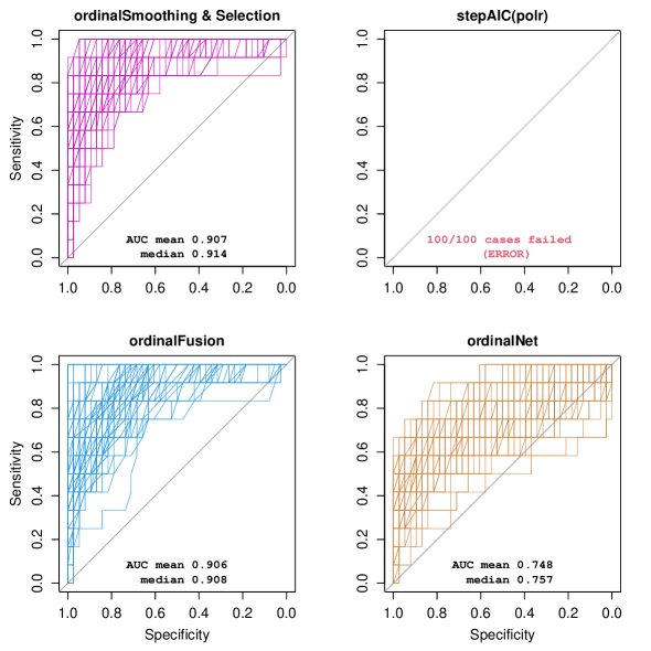
Figure S18: ROC curves when using ORS, polr, ORF or ordinalNet with n = 500. According to setting (d) from Figure S1 ($\mathbf{9}$ levels with fused effects).

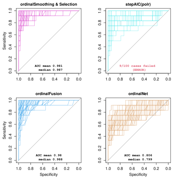
Figure S19: ROC curves when using ORS, polr, ORF or ordinalNet with n = 1000. According to setting (d) from Figure S1 ($\mathbf{9}$ levels with fused effects).

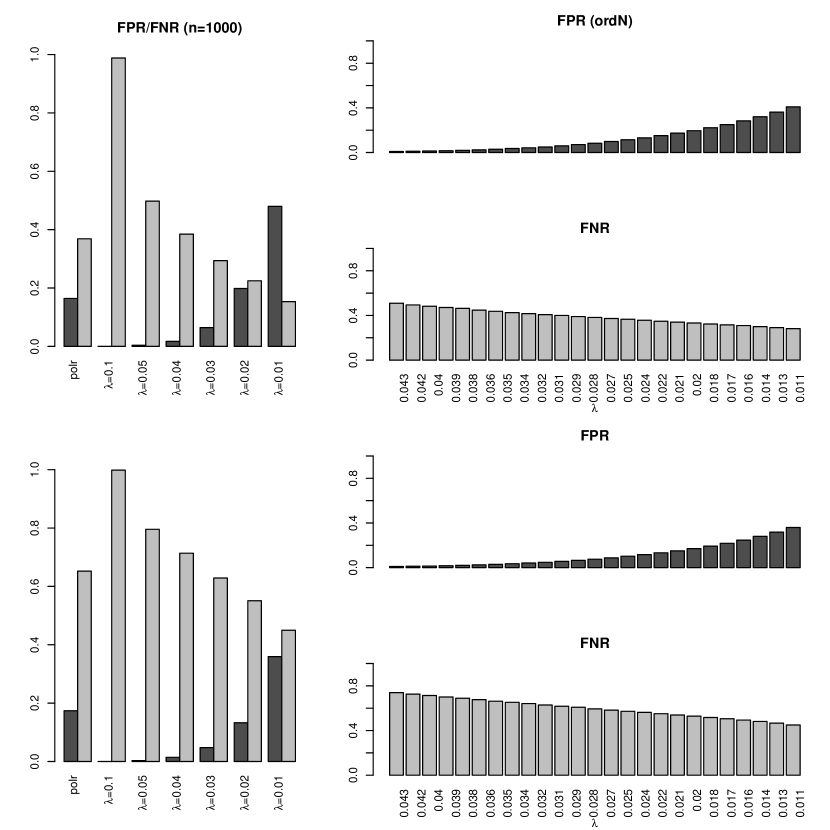
Figure S20: Evaluation of polr and ORF: false positive/negative rates (FPR/FNR) concerning identification of relevant differences (i.e., fusion) of dummy coefficients with $n=1000$. Top: $5$ levels with fused effects; bottom: $9$ levels with fused effects.

References

- Agresti (2002) Agresti, A. (2002). Categorical data. (Second ed.). Hoboken: Wiley.
- Alfnes and Sharma (2010) Alfnes, F. and A. Sharma (2010). Locally produced food in restaurants: Are the customers willing to pay a premium and why? International Journal of Revenue Management 4(3–4), 238–258.
- Brier (1950) Brier, G. W. (1950). Verification of forecasts expressed in terms of probability. Monthly weather review 78(1), 1–3.
- European Commission (2010) European Commission (2010). European declaration on alternatives to surgical castration of pigs. https://food.ec.europa.eu/system/files/2016-10/aw_prac_farm_pigs_cast-alt_declaration_en.pdf. Accessed: 2023-06-02.
- European Commission (2019) European Commission (2019). Establishing best practices on the production, the processing and the marketing of meat from uncastrated pigs or pigs vaccinated against boar taint (Immunocastrated)–Final Report. https://food.ec.europa.eu/system/files/2019-03/aw_prac_farm_pigs_cast-alt_establishing-best-practices.pdf. Accessed: 2023-06-02.
- Fahrmeir et al. (2013) Fahrmeir, L., T. Kneib, S. Lang, and B. Marx (2013). Regression: models, methods and applications. New York: Springer.
- Fahrmeir and Tutz (2001) Fahrmeir, L. and G. Tutz (2001). Multivariate statistical modelling based on generalized linear models (Second ed.). New York: Springer.
- Gertheiss et al. (2011) Gertheiss, J., S. Hogger, C. Oberhauser, and G. Tutz (2011). Selection of ordinally scaled independent variables with applications to international classification of functioning core sets. Journal of the Royal Statistical Society C 60, 377–395.
- Hartmann et al. (2016) Hartmann, L. H., S. Nitzko, and A. Spiller (2016). The significance of definitional dimensions of luxury food. British Food Journal 118(8), 1976–1998.
- Hartmann et al. (2017) Hartmann, L. H., S. Nitzko, and A. Spiller (2017). Segmentation of german consumers based on perceived dimensions of luxury food. Journal of Food Products Marketing 23(7), 733–768.
- Hoshiyar et al. (2023) Hoshiyar, A., L. Gertheiss, and J. Gertheiss (2023). Spending on luxury food. Zenodo. URL https://zenodo.org/record/8383248.
- Leng et al. (2006) Leng, C., Y. Lin, and G. Wahba (2006). A note on the lasso and related procedures in model selection. Statistica Sinica, 1273 – 1284.
- Meier (2020) Meier, L. (2020). grplasso: fitting user-specified models with group lasso penalty. R package version 0.4-7.
- Meier et al. (2008) Meier, L., S. Van De Geer, and P. Bühlmann (2008). The group lasso for logistic regression. Journal of the Royal Statistical Society: Series B 70(1), 53–71.
- Meier-Dinkel et al. (2016) Meier-Dinkel, L., J. Gertheiss, W. Schnäckel, and D. Mörlein (2016). Consumers’ perception and acceptance of boiled and fermented sausages from strongly boar tainted meat. Meat science 118, 34–42.
- Meinshausen and Bühlmann (2006) Meinshausen, N. and P. Bühlmann (2006). High-dimensional graphs and variable selection with the Lasso. The Annals of Statistics 34(3), 1436 – 1462.
- Meinshausen and Bühlmann (2010) Meinshausen, N. and P. Bühlmann (2010). Stability selection. Journal of the Royal Statistical Society: Series B 72(4), 417–473.
- Parsa et al. (2017) Parsa, H., K. Dutta, and D. Njite (2017). Consumer behaviour in restaurants: Assessing the importance of restaurant attributes in consumer patronage and willingness to pay. In V. Jauhari (Ed.), Hospitality Marketing and Consumer Behavior, pp. 211–239. Waretown: Apple Academic Press.
- R Core Team (2021) R Core Team (2021). R: a language and environment for statistical computing. Vienna: R Foundation for Statistical Computing.
- Shirai (2015) Shirai, M. (2015). Impact of "high quality, low price" appeal on consumer evaluations. Journal of Promotion Management 21(6), 776–797.
- Tibshirani et al. (2005) Tibshirani, R., M. Saunders, S. Rosset, J. Zhu, and K. Knight (2005). Sparsity and smoothness via the fused lasso. Journal of the Royal Statistical Society: Series B 67(1), 91–108.
- Tseng and Yun (2009) Tseng, P. and S. Yun (2009). A coordinate gradient descent method for nonsmooth separable minimization. Mathematical Programming 117(1), 387–423.
- Tutz (2022) Tutz, G. (2022). Ordinal regression: A review and a taxonomy of models. Wiley Interdisciplinary Reviews: Computational Statistics 14(2), e1545.
- Tutz and Gertheiss (2014) Tutz, G. and J. Gertheiss (2014). Rating scales as predictors–the old question of scale level and some answers. Psychometrika 79(3), 357–376.
- Tutz and Gertheiss (2016) Tutz, G. and J. Gertheiss (2016). Regularized regression for categorical data. Statistical Modelling 16(3), 161–200.
- Venables and Ripley (2002) Venables, W. N. and B. Ripley (2002). Modern applied statistics with S (Fourth ed.). New York: Springer.
- Walter et al. (1987) Walter, S. D., A. R. Feinstein, and C. K. Wells (1987). Coding ordinal independent variables in multiple regression analyses. American Journal of Epidemiology 125(2), 319–323.
- Wiedmann et al. (2009) Wiedmann, K., N. Hennigs, and A. Siebels (2009). Value-based segmentation of luxury consumption behavior. Psychology and Marketing 26(7), 625–651.
- Wurm et al. (2021) Wurm, M. J., P. J. Rathouz, and B. M. Hanlon (2021). Regularized ordinal regression and the ordinalNet R package. Journal of Statistical Software 99(6), 1–42.
- Yuan and Lin (2006) Yuan, M. and Y. Lin (2006). Model selection and estimation in regression with grouped variables. Journal of the Royal Statistical Society: Series B 68(1), 49–67.